Hyperspherical three-body model calculation for the bound ^1,3S-states of Coulombic systems

Abstract

In this paper, hyperspherical three-body model formalism has been applied for the calculation energies of the low-lying bound ^1,3S (L=0)-states of neutral helium and helium like Coulombic three-body systems having nuclear charge (Z) in the range Z=2 to Z=92. The calculation of the coupling potential matrix elements of the two-body potentials has been simplified by the introduction of Raynal-Revai Coefficients (RRC). The three-body wave function in the Schrődinger equation when expanded in terms of hyperpherical harmonics (HH), leads to an infinite set of coupled differential equation (CDE). For practical reason the infinite set of CDE is truncated to a finite set and are solved by an exact numerical method known as renormalized Numerov method (RNM) to get the energy solution (E). The calculated energy is compared with the ones of the literature.

Keywords: Raynal Revai Coefficient, Hyperspherical Harmonics,
         Coupled Differential Equation, Potential Matrix Elements,
         Renormalized Numerov Method.
         PACS: 02.70.-c, 31.15.-Ar, 31.15.Ja, 36.10.Ee.

1 Introduction

In physics, role of few-body (two- or three-body) problems are very important for the proper understanding of the physics underlying the internal configurations and kinematics of more complex many-body systems, usually made of interacting bosons and (or) fermions. As few-body systems are the building blocks of more complex many-body systems, they are important not only in nuclear, particle, plasma, astro-nuclear or hyper-nuclear physics but in atomic physics as well. For example, the lightest few-body systems like neutral helium atom and helium-like ions have long history as subject of attraction for both theoretical and experimental investigations. These atomic systems constituting the simplest few-body problems in atomic physics are traditionally used as testing ground for different methods of description of the structure of atoms. On the experimental side, small natural line widths of transition among various metastable quantum states of helium-like systems allow spectroscopic measurements of very high precision. In addition, few-body systems made up of electrons, protons, muons, deuteron, kaon etc. and their antimatters are found to be of strong interest in many areas of physics including atomic spectroscopy, quantum electrodynamics, particle physics and astrophysics [1-2]. In recent years, highly ionized atoms are being studied extensively to explain the origin of X-rays spectra from the solar corona and other astrophysical plasmas. It is worth mentioning here that highly ionized atoms can be produced in the laboratory by collision of ions with atoms or directing energetic projectile beams towards matter foils and their spectra can also be studied in the laboratory.

A number of theoretical methods have been adopted to investigate the bound state properties of atomic few-body systems. For example, we may refer the works of Lin [3-5], Lin et al [6] in which the author(s) has (have) applied hyperspherical coordinates to Coulombic three-body systems to calculate channel potential, channel function, binding energies and some other observables of the systems. Huang [7] investigated muonic helium atom as a three-body problem in correlated wave function approach. Some more works which may be referred here include those found in references [8-17]. Rajaraman et al [18] presented results of three-body problems originated in the nuclear matter. Alexander et al [19] reported analytical results for the trimmer binding energies and other three-body parameters considering three-body system of identical bosonic atoms. Frolov [20] adopted exponential expansion based variational approach to construct highly accurate wave functions for the triplet spin states of helium like two-electron ions like Li⁺ (atomic number Z=3] to Ne⁸⁺ (atomic number Z=10]. The ground state properties of some two-electron and electron-muon atomic three-body systems has been studied by Rodriguez et al [21] applying the Angular Correlated Configuration Interaction (ACCI) approach. The calculated energy for negatively charged hydrogen-like systems; neutral helium-like systems, and positively charged lithium like systems. However, more accurate results for these systems are reported by Smith Jr et al [22], Frolov et al [23-31], Thakkar and Koga [32], Goldman [33], Korobov [34] and Drake [35]. Researchers like- Hylleraas and Ore [36], Hill [37], Mohr and Taylor [38], Drake, Cassar and Razvan [39], Frolov [40], Mills [41-42], Ho [43-44] and Wen-Fang [45] have explored the bound state properties of exotic positronium negative ion $Ps^{-}(e^{+}e^{-}e^{-})$. Ancarani et al [1-2] also reported the ground and excited state energies for several three-body atomic systems obtained by applying ACCI approach. Kubicek et al [46] and Kondrashev et al [47] conducted experiments on production of He-like ions. In this paper we present energies of the low-lying bound ^1,3S-states of neutral helium and helium like two-electron Coulombic three-body systems having nuclear charge number Z in the range Z=2 - 92. The resulting three-body Schrőodinger equation has been solved in the framework of hyperspherical harmonics expansion (HHE) formalism applying an exact numerical method known as renormalized Numerov method (RNM) [48]. The scheme of solution of the three-body Schrődinger equation in HHE approach has been described in more details in our earlier works [49-62]. In HHE approach for a general three-body system containing particles of arbitrary masses, there are three possible partitions and in the $i^{th}$ partition, the particle labeled $i$, acts as a spectator while the remaining two, labeled $j$ and $k$ form the interacting pair. For the calculation matrix element of the potential of the $(jk)$ pair, V($r_{jk}$), it is convenient to expand the chosen HH in the set of HH corresponding to the partition in which the potential $\vec{r_{jk}}$ is proportional to the first Jacobi vector $\vec{\xi_{i}}$ [49] and this has been done using Raynal-Revai coefficients (RRC) [63]. In the numerical procedure of computation of potential matrix elements of the two-body potentials involved in the system of three particles constituted by a relatively heavy and positively charged nucleus being orbited by two valence electrons, we used RRC of [49,64]. The energies of the low-lying bound ^1,3S-states of several Coulombic three-body systems obtained by solving the three-body Schrödinger equation have been compared with the ones of the literature.

In Section 2, we will give a very concise description of the HHE method along with the scheme of transformation between two sets of HH which correspond to two different partitions. In Section 3, we will discuss the application of HHE to the low-lying bound spin singlet (spin S=0) and spin triplet (spin S=1) i.e. ^1,3S (L=0)-states of neutral helium and similar other systems to calculate the energies and compare them with the ones of the literature.

2 HHE Method

In the hyperspherical harmonics expansion (HHE) method for a general three-body system of particles of arbitrary masses $m_{i}$, $m_{j}$, $m_{k}$ as depicted in Figure 1,

Figure 1: Particle label scheme for general three-body system and choice of Jacobi coordinates in the $i^{th}$ partition.

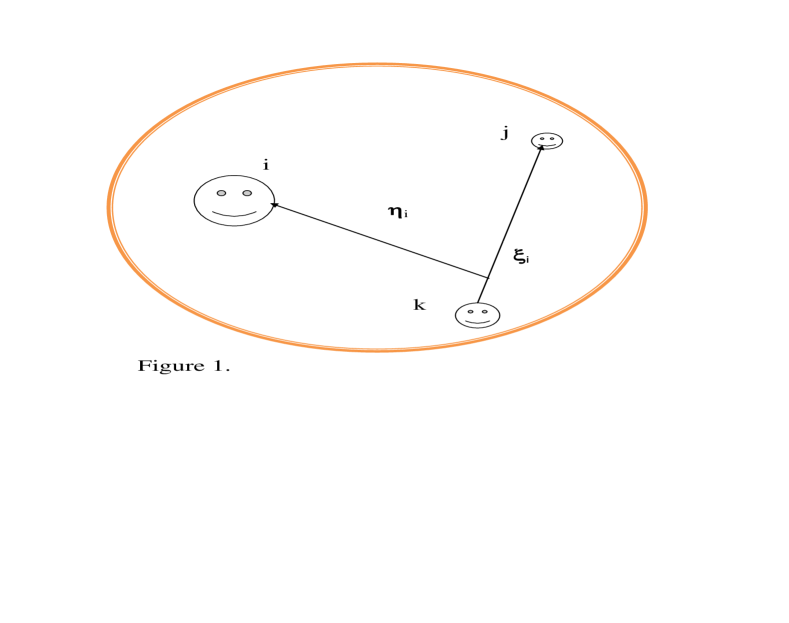
the Jacobi coordinates [64] in the partition - $``i$" are defined as

$$\left.\begin{array}[]{ccl}\vec{\xi_{i}}&=&\left[\frac{m_{j}m_{k}M}{m_{i}(m_{j}+m_{k})^{2}}\right]^{\frac{1}{4}}(\vec{r_{j}}-\vec{r_{k}})\\ \vec{\eta_{i}}&=&\left[\frac{m_{i}(m_{j}+m_{k})^{2}}{m_{j}m_{k}M}\right]^{\frac{1}{4}}\left(\vec{r_{i}}-\frac{m_{j}\vec{r_{j}}+m_{k}\vec{r_{k}}}{m_{j}+m_{k}}\right)\end{array}\right\}$$ (1)

where $M=m_{i}+m_{j}+m_{k}$ and the condition that ($i,j,k$) should form a cyclic permutation of (1, 2, 3) determines the sign of $\vec{\xi_{i}}$.
The set of Jacobi coordinates represented by eq.(1) above corresponds to the partition, in which, the particle labeled $``i$" is the spectator and the remaining particles labeled $``j$" and $``k$" form the interacting pair. The reason behind such nomenclature is that the calculation of matrix element of V$(\vec{r}_{jk})$ in terms of the above set of Jacobi coordinates is straight forward. In the similar manner, we can also define two other sets of Jacobi coordinates by cyclically permuting $i\rightarrow j\rightarrow k\rightarrow i$ twice, which correspond to $j^{th}$ and $k^{th}$ partitions respectively.
In hyper-spherical variables [65-66] of the $i^{th}$ partition, three-body Schrődinger equation is

$$\left[-\frac{\hbar^{2}}{2\mu\rho^{5}}\frac{\partial}{\partial\rho}(\rho^{5}\frac{\partial}{\partial\rho})+\frac{\hbar^{2}}{2\mu\rho^{2}}\frac{\hat{{\cal N}}^{2}(\Omega_{i})}{\rho^{2}}+V(\rho,\Omega_{i})-E\right]\Psi(\rho,\Omega_{i})\>=\>0$$ (2)

where ${\mu\>=\>\left[\frac{m_{i}m_{j}m_{k}}{M}\right]^{\frac{1}{2}}}$ is an effective mass parameter, $V(\rho,\Omega_{i})$ = $V_{jk}+V_{ki}+V_{ij}$ is the total interaction potential, and $\hat{\cal N}^{2}(\Omega_{i})$ is the square of the hyper angular momentum operator satisfying the eigenvalue equation [67]

$$\hat{{\cal N}}^{2}(\Omega_{i}){\cal H}_{N\alpha_{i}}(\Omega_{i})\>=\>N(N+4){\cal H}_{N\alpha_{i}}(\Omega_{i})$$ (3)

where

$$\begin{array}[]{rcl}{\cal H}_{N\alpha_{i}}(\Omega_{i})&\equiv&{\cal H}_{Nl_{\xi_{i}}l_{\eta_{i}}LM}(\phi_{i},\theta_{\xi_{i}},\phi_{\xi_{i}},\theta_{\eta_{i}},\phi_{\eta_{i}})\\ &\equiv&{}^{(2)}P_{N}^{l_{\xi_{i}}l_{\eta_{i}}}(\phi_{i})\left[Y_{l_{\xi_{i}}m_{\xi_{i}}}(\theta_{\xi_{i}},\phi_{\xi_{i}})Y_{l_{\eta_{i}}m_{\eta_{i}}}(\theta_{\eta_{i}},\phi_{\eta_{i}})\right]_{LM}\end{array}$$ (4)

is the normalized eigenfunction known as hyperspherical harmonics (HH), $L$ is the total orbital angular momentum of the system with $M$ as its projection, $\Omega_{i}\rightarrow\{\phi_{i},\theta_{\xi_{i}},\phi_{\xi_{i}},\theta_{\eta_{i}},\phi_{\eta_{i}}\}$, ${\alpha_{i}\>\equiv\>\{l_{\xi_{i}},l_{\eta_{i}},L,M\}}$ is a short hand notation and $[]_{LM}$ indicates angular momentum coupling. The quantity $N=2n_{i}+l_{\xi_{i}}+l_{\eta_{i}}$ ($n_{i}$ being a non-negative integer) is the hyper-angular momentum quantum number which is not a good quantum number for the three-body system. In terms of HH associated with a given partition, (say partition $``i$), the wave-function $\Psi(\rho,\Omega_{i})$ is expanded in the complete set of HH

$$\Psi(\rho,\Omega_{i})=\sum_{N\alpha_{i}}\frac{U_{N\alpha_{i}}(\rho)}{\rho^{5/2}}{\cal H}_{N\alpha_{i}}(\Omega_{i})$$ (5)

Substitution of eq.(5) in eq.(2), use of eq.(3) and the ortho-normality of HH, leads to a set of coupled differential equations (CDE) in $\rho$

$$\begin{array}[]{cl}&\left[-\frac{\hbar^{2}}{2\mu}\frac{d^{2}}{d\rho^{2}}+\frac{\hbar^{2}}{2\mu}\frac{(N+3/2)(N+5/2)}{\rho^{2}}-E\right]U_{N\alpha_{i}}(\rho)\\ +&\sum_{N^{\prime}\alpha_{i}^{~{}\prime}}<N\alpha_{i}\mid V(\rho,\Omega_{i})\mid N^{\prime}\alpha_{i}^{~{}\prime}>U_{N^{\prime}\alpha_{i}^{~{}\prime}}(\rho)\>=\>0.\end{array}$$ (6)

where

$$<N\alpha_{i}|V|N^{\prime},\alpha_{i}^{\prime}>=\int{\cal H}_{N\alpha_{i}}^{*}(\Omega_{i})V(\rho,\Omega_{i}){\cal H}_{N^{\prime}\alpha_{i}^{~{}\prime}}(\Omega_{i})d\Omega_{i}$$ (7)

For central potentials, computation of the matrix elements of the form

$$<{\cal H}_{N\alpha_{i}}(\Omega_{i})\mid V_{jk}(\xi_{i})\mid{\cal H}_{N^{\prime}\alpha_{i}^{\prime}}(\Omega_{i})>$$

is straight forward, while for matrix elements of the forms

$$<{\cal H}_{N\alpha_{i}}(\Omega_{i})\mid V_{ki}(\xi_{j})|{\cal H}_{N^{\prime}\alpha_{i}^{~{}\prime}}(\Omega_{i})>$$

or

$$<{\cal H}_{N\alpha_{i}}(\Omega_{i})\mid V_{ij}(\xi_{k})\mid{\cal H}_{N^{\prime}\alpha_{i}^{~{}\prime}}(\Omega_{i})>$$

computations become very complicated even for central potentials. This is because the vectors $\vec{\xi_{j}}$ or $\vec{\xi_{k}}$ depend on the polar angles of the vectors $\vec{\xi_{i}}$ and $\vec{\eta_{i}}$. Vectors $\vec{\xi_{k}}$ and $\vec{\eta_{k}}$ can be expressed in terms of $\vec{\xi_{i}}$ and $\vec{\eta_{i}}$ using eq.(1) as

$$\left.\begin{array}[]{rcl}\vec{\xi_{k}}&=&-\cos\sigma_{ki}\vec{\xi_{i}}+\sin\sigma_{ki}\vec{\eta_{i}}\\ \vec{\eta_{k}}&=&-\sin\sigma_{ki}\vec{\xi_{i}}-\cos\sigma_{ki}\vec{\eta_{i}}\end{array}\right\}$$ (8)

where $\sigma_{ki}$ = $\tan^{-1}\{(-1)^{P}\sqrt{\frac{Mm_{j}}{m_{i}m_{k}}}\}$, P being even (odd) if ($kij$) is an even (odd) permutation of the triad (1 2 3). Now for any arbitrary shape of the central potential with non-vanishing L, most of the five dimensional integrals have to be done numerically which makes the calculation time consuming and inaccurate. However computation of the latter matrix elements can be greatly simplified using the following prescription. At first it is to be noted that each of the complete sets of HH $\{{\cal H}_{N\alpha_{i}}(\Omega_{i})\}$, $\{{\cal H}_{N\alpha_{j}}(\Omega_{j})\}$ or $\{{\cal H}_{N\alpha_{k}}(\Omega_{k})\}$ span the same five dimensional angular hyperspace. Then a particular member of a given set, say ${\cal H}_{N\alpha_{i}}(\Omega_{i})$ can be expanded in the complete set of $\{{\cal H}_{N\alpha_{k}}(\Omega_{k})\}$ through a unitary transformation:

$${\cal H}_{N\alpha_{i}}(\Omega_{i})=\sum_{\alpha_{k}}<\alpha_{k}\mid\alpha_{i}>_{NL}{\cal H}_{N\alpha_{k}}(\Omega_{k})$$ (9)

As $N,L,M$ are conserved for eq.(9) and there is rotational degeneracy with respect to the quantum number $M$ for spin independent forces, we have

$$<\alpha_{k}\mid\alpha_{i}>_{NL}=<l_{\xi_{k}}l_{\eta_{k}}\mid l_{\xi_{i}}l_{\eta_{i}}>_{NL}$$ (10)

Thus, eq.(9) can be rewritten as [52]

$${\cal H}_{N\alpha_{i}}(\Omega_{i})=\sum_{l_{\xi_{k}}l_{\eta_{k}}}<l_{\xi_{k}}l_{\eta_{k}}\mid l_{\xi_{i}}l_{\eta_{i}}>_{NL}{\cal H}_{N\alpha_{k}}(\Omega_{k})$$ (11)

The coefficients involved in eq.(10) and (11) are called the Raynal-Revai Coefficients (RRC) and these are independent of M due to overall rotational degeneracy. In terms of these coefficients, the matrix element of a central interaction $V_{ij}$ then becomes

$$\begin{array}[]{ll}&<{\cal H}_{N\alpha_{i}}(\Omega_{i})\mid V_{ij}(\xi_{k})\mid{\cal H}_{N^{\prime}\alpha_{i}^{\prime}}(\Omega_{i})>\\ =&\sum_{l_{\xi_{k}}^{\prime}l_{\eta_{k}}^{\prime}l_{\xi_{k}}l_{\eta_{k}}}<l_{\xi_{k}}l_{\eta_{k}}\mid l_{\xi_{i}}l_{\eta_{i}}>_{NL}^{*}\times<l_{\xi_{k}}^{\prime}l_{\eta_{k}}^{\prime}\mid l_{\xi_{i}}^{\prime}l_{\eta_{i}}^{\prime}>_{N^{\prime}L}\\ \times&<{\cal H}_{N\alpha_{k}}(\Omega_{k})\mid V_{ij}(\xi_{k})\mid{\cal H}_{N^{\prime}\alpha_{k}^{\prime}}(\Omega_{k})>\end{array}$$ (12)

The matrix element on the right side of eq.(12) has the same form as the matrix element of $V_{jk}$ in the partition $i$ and can be calculated in a straight forward manner. Thus computing the values of RRC’s involved in eq.(12) using their explicit expressions found in [49, 63], one can calculate the matrix element of $V_{ij}$ easily. Similar prescription can also be employed for the calculation of the matrix element of $V_{ki}$.

3 Application to Coulombic three-body systems

We apply the scheme of RRC to the low-lying bound ^1,3S (L=0)-states of Coulombic three-body system containing relatively massive and positively charged nuclear core plus two extra core orbital electrons. We label the nuclear core having mass $m_{C}$ and charge +Ze as the $i^{th}$ particle, two electrons of mass $m_{j}=m_{k}=m$ and charge -e as the $j^{th}$ and $k^{th}$ particles respectively. For this particular choice mass of the system particles, Jacobi coordinates of eq.(1) in corresponding to the partition $i$ becomes

$$\left.\begin{array}[]{rcl}\vec{\xi_{i}}&=&\beta_{i}(\vec{r_{j}}-\vec{r_{k}})\\ \vec{\eta_{i}}&=&\frac{1}{\beta_{i}}(r_{i}-\frac{\vec{r_{j}}+\vec{r_{k}}}{2})\end{array}\right\}$$ (13)

where the dimensionless parameter $\beta_{i}$ = $\left[\frac{m_{C}+2m}{4m_{C}}\right]^{\frac{1}{4}}$ can be connected to the effective mass $\mu$ as

$$\begin{array}[]{cclcl}\mu&=&m\left(\frac{m_{C}}{m_{C}+2m}\right)^{\frac{1}{2}}&=&\frac{m}{2\beta_{i}^{2}}\end{array}$$ (14)

In atomic unit (ie., $\hbar^{2}$=$m$=$e^{2}$=1), eq.(6) becomes

$$\left.\begin{array}[]{lcl}\left[-\beta_{i}^{2}\frac{d^{2}}{d\rho^{2}}+\beta_{i}^{2}\frac{(N+3/2)(N+5/2)}{\rho^{2}}-E\right]U_{N\alpha_{i}}(\rho)&&\\ +\sum_{N^{\prime}\alpha_{i}^{\prime}}<N\alpha_{i}\mid\frac{\beta_{i}}{\rho cos\phi_{i}}-\frac{Z}{\rho\left|(\beta_{i}sin\phi_{i})\hat{\eta_{i}}-(\frac{1}{2\beta_{i}}cos\phi_{i})\hat{\xi_{i}}\right|}&&\\ -\frac{Z}{\rho\left|(\beta_{i}sin\phi_{i})\hat{\eta_{i}}+(\frac{1}{2\beta_{i}}cos\phi_{i})\hat{\xi_{i}}\right|}\mid N^{\prime}\alpha_{i}^{\prime}>U_{N^{\prime}\alpha_{i}^{\prime}}(\rho)&=&0\end{array}\right\}$$ (15)

Mass of the particles involved in the present calculation is partly taken from [1-2, 28-30, 68-69]. A straight forward evaluation of the matrix elements of last two terms in eq.(15) would be prohibitively involved both for analytical reduction to a computationally feasible form, as well as for the numerical calculation. Furthermore, the numerical calculation would be both inaccurate and time consuming. Application of RRC greatly simplifies the calculation, since in the partitions $k$ and $j$, the third and fourth terms inside ket-bra <> notation in eq.(15) is reduced to $\frac{Z\beta_{k}}{\rho cos\phi_{k}}$ and $\frac{Z\beta_{j}}{\rho cos\phi_{j}}$ respectively. In the case of two-electron ions,

$$\begin{array}[]{ccccl}\beta_{j}&=&\beta_{k}&=&\left[1-\frac{m^{2}}{(m_{C}+m)^{2}}\right]^{\frac{1}{4}}\end{array}$$ (16)

In the case of a heavy nucleus, ${m_{C}\gg m}$ and ${\beta_{i}\approx\frac{1}{\sqrt{2}}}$, ${\beta_{j}=\beta_{k}\simeq}$ 1.

We expand the three-body relative wave function in the complete set of HH appropriate to the partition $i$ according to eq.(5). For the low-lying ^1,3S-states of two-electron systems the total orbital angular momentum, $L$=0. Consequently ${l_{\xi_{i}}=l_{\eta_{i}}}$. Hence the set of quantum numbers represented by $\alpha_{i}$ is ${\left\{l_{\xi_{i}},l_{\xi_{i}},0,0\right\}}$ and the quantum numbers ${\left\{N\alpha_{i}\right\}}$ can be represented by ${\left\{Nl_{\xi_{i}}\right\}}$ only. Furthermore for S=0, spin part of the two-electron wave function is anti-symmetric, hence the space part of the wave function must be symmetric under exchange of two electrons which allows only even values of $l_{\xi_{i}}$ ($\leq N/2$). On the other hand for S=1, spin part of the wave function is symmetric, hence space part of the wave function must be anti-symmetric under the exchange of the two electrons which allows only odd values of $l_{\xi_{i}}$ ($\leq N/2$) are to be considered. Corresponding HH is then given by [65]

$$\left.\begin{array}[]{ccl}{\cal H}_{N\alpha_{i}}(\Omega_{i})&\equiv&{\cal H}_{Nl_{\xi_{i}}l_{\xi_{i}}00}(\Omega_{i})\\ &=&{}^{(2)}P_{N}^{l_{\xi_{i}}l_{\xi_{i}}}(\phi_{i})\left[Y_{l_{\xi_{i}}m_{\xi_{i}}}(\theta_{\xi_{i}},\phi_{\xi_{i}})Y_{l_{\xi_{i}}-m_{\xi_{i}}}(\theta_{\xi_{i}},\phi_{\xi_{i}})\right]_{00}\\ &&N\>even\>and\>l_{\xi_{i}}=0,2,4,\ldots,\leq N/2\>for\>^{1}S\>states;\\ &&l_{\xi_{i}}=1,3,5,\ldots,\leq N/2\>for\>^{3}S\>states\end{array}\right\}$$ (17)

The matrix element of the two electron repulsion term in our chosen partition $i$ is

$$\begin{array}[]{rcl}<N^{\prime}l_{\xi_{i}}^{\prime}|\frac{\beta_{i}}{\rho cos\phi_{i}}|Nl_{\xi_{i}}>&=&\frac{\beta_{i}}{\rho}\delta_{l_{\xi_{i}}^{\prime},l_{\xi_{i}}}\int_{0}^{\pi/2}{{}^{(2)}P_{K^{\prime}}}^{l_{\xi_{i}}l_{\xi_{i}}}(\phi)\\ &&\times{{}^{(2)}P_{N}}^{l_{\xi_{i}}l_{\xi_{i}}}(\phi)\sin^{2}\phi\cos\phi d\phi\\ \end{array}$$ (18)

in which suffix $i$ on $\phi$ has been dropped deliberately as it is only a variable of integration. Similarly the matrix element of the third term of the total potential in eq.(15) in the partition $k$ is

$$\begin{array}[]{rcl}<N^{\prime}l_{\xi_{k}}^{\prime}\mid\frac{\beta_{k}}{\rho cos\phi_{k}}\mid Nl_{\xi_{k}}>&=&\frac{\beta_{k}}{\rho}\delta_{l_{\xi_{k}}^{\prime},l_{\xi_{k}}}\int_{0}^{\pi/2}{{}^{(2)}P_{N^{\prime}}}^{l_{\xi_{k}}l_{\xi_{k}}}(\phi)\\ &&\times{{}^{(2)}P_{N}}^{l_{\xi_{k}}l_{\xi_{k}}}(\phi)\sin^{2}\phi\cos~{}\phi~{}d\phi\\ \end{array}$$ (19)

A similar relation holds for the matrix element of the last term of the total potential in eq. (15) in the partition $j$. Eq.(18) and (19) show that the matrix elements are essentially the same in the respective partitions, although $l_{\xi_{k}}$ and $l_{\xi_{j}}$ are not restricted to only even or odd integer values. Each involves only a single, one dimensional integral to be performed numerically. Using eq.(12), matrix elements of the third and fourth terms of the total potential in eq.(15) in the partition $i$ become

$$\begin{array}[]{rcl}<N^{\prime}l_{\xi_{i}}^{\prime}\mid\frac{Z}{r_{ij}}\mid Nl_{\xi_{i}}>&=&\sum_{l_{\xi_{k}}}<l_{\xi_{k}}l_{\xi_{k}}\mid l_{\xi_{i}}^{\prime}l_{\xi_{i}}^{\prime}>_{K^{\prime}0}^{\*}<l_{\xi_{k}}l_{\xi_{k}}\mid l_{\xi_{i}}l_{\xi_{i}}>_{N0}\\ &&<K^{\prime}l_{\xi_{k}}\mid\frac{Z\beta_{k}}{\rho cos\phi_{k}}\mid Kl_{\xi_{k}}>.\end{array}$$ (20)

and

$$\begin{array}[]{rcl}<N^{\prime}l_{\xi_{i}}^{\prime}\mid\frac{Z}{r_{ik}}\mid Nl_{\xi_{i}}>&=&\sum_{l_{\xi_{j}}}<l_{\xi_{j}}l_{\xi_{j}}\mid l_{\xi_{i}}^{~{}\prime}l_{\xi_{i}}^{\prime}>_{N^{\prime}0}^{\*}<l_{\xi_{j}}l_{\xi_{j}}\mid l_{\xi_{i}}l_{\xi_{i}}>_{N0}\\ &&<N^{\prime}l_{\xi_{j}}\mid\frac{Z\beta_{j}}{\rho cos\phi_{j}}\mid Nl_{\xi_{j}}>.\end{array}$$ (21)

In eq.(20) and (21) sums over $l_{\xi_{k}}^{\prime}$ and $l_{\xi_{j}}^{\prime}$ respectively have been performed using the Kronecker - $\delta$’s in eq.(19) and a similar one with suffix $k$ replaced by suffix $j$. Thus the calculation of the matrix elements of $\underline{all}$ the interactions become practically simple and easy to handle numerically.

Although the rate of convergence of HH expansion is reasonably fast [70] for short-range interaction potentials [67, 70-71], the same cannot be claimed for long-range coulomb potentials. So to achieve desired convergence, large enough $N_{m}$ value is to be included in the calculation. In the case of singlet spin (S=0) states, if all N values up to a maximum of $N_{m}$ are retained in the HH expansion then the number of such basis function is

$$N_{B}=\left\{\begin{array}[]{l}(\frac{N_{m}}{4}+1)^{2}\>\>if\>\frac{N_{m}}{2}\>is\>even\\ \frac{(\frac{N_{m}}{2}+1)(\frac{N_{m}}{2}+3)}{4}\>\>if\>\frac{N_{m}}{2}\>is\>odd.\end{array}\right.$$ (22)

and that for the triplet spin state (S=1) is

$$N_{B}=\left\{\begin{array}[]{l}(\frac{N_{m}}{4})(\frac{N_{m}}{4}+1)\>\>if\>\frac{N_{m}}{2}\>is\>even\\ (\frac{N_{m}+2}{4})^{2}\>if\>\frac{N_{m}}{2}\>is\>odd.\end{array}\right.$$ (23)

It can be checked from eq.(22) and eq. (23) respectively, that the number of basis states ($N_{B}$) and hence the size of CDE {eq.(6)} increases rapidly as $N_{m}$ increases. For example, for $N_{m}=96$ one has to solve 625 CDE for singlet spin and 600 CDE for the triplet spin configuration respectively which lead the calculation towards instability. We used dual-core based desktop computer for the present calculation and could solve only up to $N_{m}=28$ reliably. The calculated binding energy ($B_{N_{m}}$) for values of $N_{m}$ up to 28 are presented in columns 2 -10 of Table I for few low-lying ^1,3S-states of two-electron Coulombic systems like neutral helium and highly ionized radon Rn⁸⁴⁺ and that for Rb³⁵⁺ is presented in Table 3. The energies for still higher $N_{m}(>28)$ may be obtained by following an extrapolation theorem suggested by Schneider [72] as discussed below. According to the theorem on convergence of HH one may expect following relation to hold for coulomb interaction:

$$(N_{m}+y)^{4}\Delta B_{N_{m}}=C,$$ (24)

where

$$\Delta B_{N_{m}}=E_{N_{m}+4}-B_{N_{m}}$$ (25)

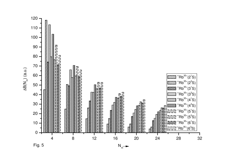
and y, C are constants. If one obtains y and C by solving eq.(24) for $N_{m}$=16 and 20 and uses eq.(24) to estimate the BE for $N_{m}=28$, he finds that the estimated BE agrees fairly well with the BE actually calculated by solving CDE with $N_{m}=28.$ In this way one may verify that eq.(24) is well obeyed. For the converged extrapolated BE (=$B_{con}=B_{N_{M}}$), we calculated the constants y and C from eq.(24) by least square fitting $B_{N_{m}}$ obtained by solving the CDE for $N_{m}=0,4,8,...,up\;to\;28$. With these values of y and C the extrapolated energies calculated by eq.(24) for larger $N_{m}$ (>28) are presented in columns 2-10 of Table 2. We select a value of $N_{m}(=N_{M})$ for which $\Delta B_{N_{m}}$ is of the same order as the overall numerical error ($\epsilon$) in the calculation of $B_{N_{m}}$ with $N_{m}\leq 28$. Since, for any $N_{m}>N_{M}$, the correction $\Delta B_{N_{M}}$ will be smaller than $\epsilon$ and hence unreliable due to the finite numerical precision in solving the CDE. We estimated $\epsilon$ to be about $4\times 10^{-5}$ for a double precision calculation using dual-core based personal computer. The corresponding extrapolated results are presented in bold in column 4 of Table 4 and in columns 4 & 7 of Tables 5-7 together with some other results including the experimental ones for the low-lying ^1,3S-states wherever available. The term exact as the subscript of E in the 5th column of Table 5 refers to the results which were obtained by highly accurate variational procedures that involved very large numbers of linear and non-linear parameters [1-2,28-30]. The calculated energies for the low-lying bound ^1,3 states for systems of different nuclear charge Z using data presented in column 3 of Table 4 and columns 3, 4 of Table 5-7 have been plotted in Figure 2 to see how the binding energies of the corresponding states depend on Z. To study the dependence of the convergence trend of calculated energy on Z, the difference in energy $\Delta B=B(N_{m}+4)-B(N_{m})$ is plotted in Figure 3 for few cases of different Z. Using the calculated energy data presented in Table 3 we have plotted Figures 4 and 5 to study the variation of the binding energy B and the quantity $\Delta B$ with increase in $N_{m}$ for ^∞Rb⁸⁴⁺. The convergence trend in energy can be checked by gradually increasing $N_{m}$ values in suitable steps and comparing the energy difference $\Delta B=B(N+dN)-B(N)$ with that obtained in the previous step. By analysis of the calculated energy data presented in Table 1, it can be said that the energy of the lowest S-states in the lightest atom under consideration converges much faster than others with respect to the increase in $N_{m}$ values. This trend of convergence with respect to the increasing $N_{m}$ is slowed down gradually which can be viewed in two ways: (I) with respect to the increase in the level of excitation keeping nuclear charge number Z fixed and (II) with respect to the increase in the nuclear charge number (Z) for a particular level of excitation. For justifying our forgoing remarks -(I) we may compare the convergence trend in energy with respect to $N_{m}$ for 2³S and 4³S states of neutral helium He (Z=2) or for the corresponding states of highly ionized radon Rn⁸⁴⁺ (Z=86) by estimating and comparing the energy difference $\Delta B=B(N_{m}=28)-B(N_{m}=24)$ using the data presented in columns 4, 6 or those presented in columns 9, 11 of Table 1. These estimates for 2³S and 4³S states of neutral helium (He) are 0.0244au, 0.0660au and those for Rn⁸⁴⁺ are 31.840au, 117.416au respectively thereby justifying our forgoing remarks -(I). Similar trends can also be seen in Figure 5 drawn for Rb³⁵⁺ as representative case using data of Table 3. For the justification of our remarks -(II), we may compare the convergence trend in energy with respect to $N_{m}$ for 4¹S state of neutral helium He (Z=2), positively charged rubidium Rb³⁵⁺ (Z=37) and highly charged radon Rn⁸⁴⁺ (Z=86) by estimating energy difference $\Delta B=B(N_{m}=28)-B(N_{m}=24)$ using the data presented in column 5 of Table 1, in column 7 of Table 3 and in column 10 of Table 1 respectively and compare them. And these estimates for 4¹S state of He, Rb³⁵⁺, Rn⁸⁴⁺ are 0.0681au, 19.220au and 102.152au respectively thereby justifying our remarks -(II). Similar results can also be found for remaining levels of excitation using data presented in Table 1-3. This trend of convergence of energy is also demonstrated in Figure 3 for few low-lying ^1,3S states of Rb³⁵⁺ and Rn⁸⁴⁺ respectively as representative cases. Furthermore it could also be noted that, although, the direct evaluation of the matrix element of ${\frac{1}{r_{ij}}}$ is possible in the partition $i$ by the method of ref. [66], it is not possible for an interaction other than Coulombic or harmonic oscillator type. For an arbitrary shape of interaction potential, a direct calculation of the matrix element of the potential will involve five dimensional angular integrations which make the calculation very time consuming and leaves door open for inaccuracies to creep in easily. Hence the use of RRC for quick and accurate computation of energy in such cases becomes inevitable.

Figure 2: Dependence of the energy, B(=-E) of the low-lying bound ^1,3S-states of helium like Coulombic three-body system ^∞X^(Z-2)+ (X=He, Li, Be, C, etc.) on the increase in nuclear charge Z. [Data source: Table 4-7]

Figure 3: Dependence of the energy difference $\Delta B=B(N_{m}+4)-B(N_{m})$ on the increase in $N_{m}$ for few low-lying bound ^1,3S-states of helium like Coulombic three-body systems having different nuclear core charge Z. [Data source: Table 1 & 3]

Figure 4: Dependence of the energy B (=-E) on the increase in $N_{m}$ for few low-lying bound ^1,3S-states of ^∞Rb³⁵⁺ ion. [Data source: Table 3]

Figure 5: Dependence of the energy difference $\Delta B=B(N_{m}+4)-B(N_{m})$ on the increase in $N_{m}$ for few low-lying bound ^1,3S-states of ^∞Rb³⁵⁺ ion. [Data source: Table 3]

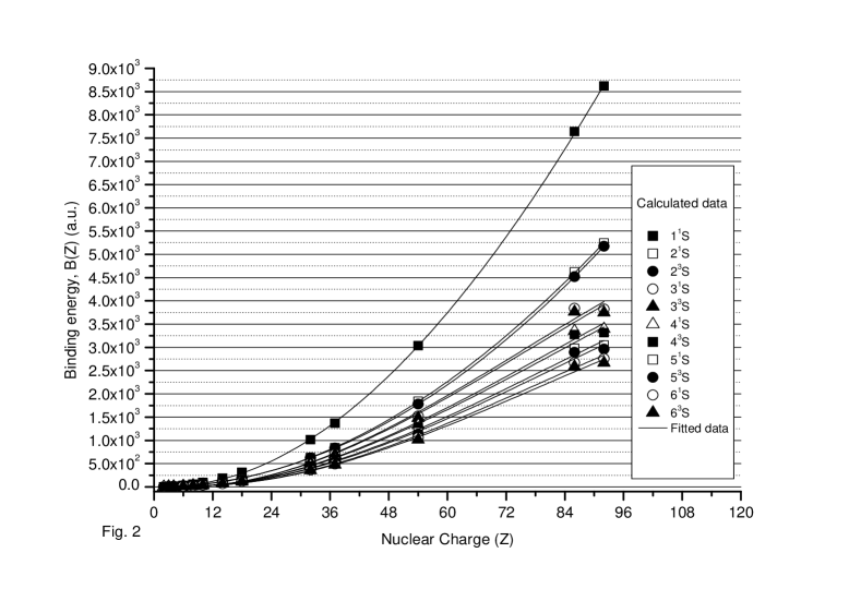
One may see from Figure 2, that the calculated energy increases gradually with the increase in the charge number (Z) of the nuclear core of helium like Coulombic three-body systems ^∞X^(Z-2)+ (X=He, Li, Be, C,….,U). An approximate value of the energy of the low-lying bound ^1,3S-states of any two-electron three-body system with a given Z can be estimated following empirical formula using the appropriate set of values of parameters $p_{0},p_{1},p_{2},p_{3}$ recorded in Table 8

$$B(Z) = \sum_{j=0}^{3}p_{j}Z^{j}$$ (26)

The values of the parameters $p_{0},p_{1},p_{2},p_{3}$ presented in Table 8 are obtained by fitting the calculated energy data presented in Table 4 to Table 7 for the low-lying bound ^1,3S-states of two-electron Coulombic three-body systems having nuclear charge (Z) in the range Z=2 to Z=92.

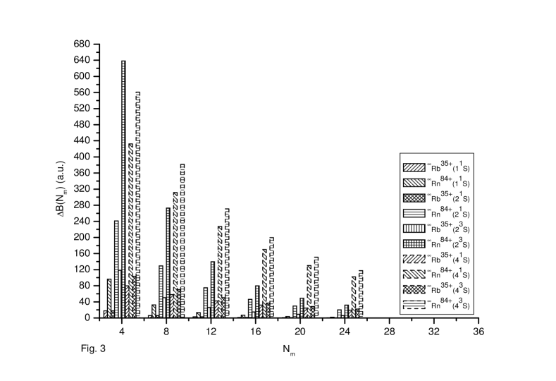
Figure 3 indicates that the rate of convergence in energy with respect to the gradual increase in the size of the basis states $N_{m}$ in the case of Rn⁸⁴⁺ (Z=86) is slower than that for Rb³⁵⁺ (Z=37). This convergence trend can be checked by observing the relative decrement in the height of the bars corresponding to a particular level of excitation of Rb³⁵⁺ and Rn⁸⁴⁺ and comparing them with respect to gradually increasing values of $N_{m}$. For example, the height of the extreme left bar representing 1¹S state of Rb³⁵⁺ decreases quicker than the height of the bar on its adjacent right representing 1¹S state of Rn⁸⁴⁺ with increasing values of $N_{m}$. Similar observations hold for other quantum states (or levels of excitation) of the systems.

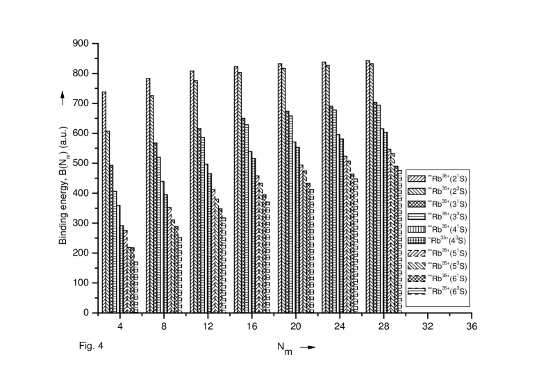
Further we have plotted in Figures 4 and 5 the variation of binding energy B, and the quantity $\Delta B$ against $N_{m}$ for different low-lying bound ^1,3S-states of Rb³⁵⁺ ion as a representative case to study the convergence trend of energy of the low-lying bound S-states of a system with fixed Z using the data of Table 3. And it is observed from Figures 4 and 5, that the energies obtained for relatively lower levels converges earlier than the higher ones. Finally in Tables 4-7, the energies of the low-lying bound ^1,3S-states for several Coulombic three-body systems obtained by solving the truncated set of coupled differential equations by the renormalized Numerov method [48] in the framework of HHE aided by RRC, have been compared with the ones of the literature.

4 Conclusion

In conclusion, we note that the use of RRC in HHE method becomes inevitable for the solution of the three-body Schrődinger equation, if the inter-particle interaction is other than Coulomb or harmonic type. Hence these coefficients are of immense importance for any type of interaction involved in three-body calculation. However in Tables 4, the calculated energy of the bound ^1,3 S-state at $N_{m}$=28 in most cases are smaller than those listed in column 5 & 6. This is due to the eventual truncation of expansion basis to a maximum value of N up to $N_{m}$=28 due to computer memory limitation. However, one may extrapolate the calculated energy values for $N_{m}$=0, 4, 8,… etc. to get the solution for still higher $N_{m}$>28 which have been described in the previous section and the corresponding extrapolated data (for $N_{m}$>$28$) have been demonstrated in Table 2 for few low-lying S-states of He and Rn as representative cases. The extrapolated energy values (at $N_{m}$=$N_{M}$) are listed in bold in the $4^{th}$ column of Table 4 and in columns 4,7 of Tables 5-7. The extrapolated energies agree fairly well with the corresponding exact values found in the literature. One of the important aspect of RRC’s are that they are independent of r, and need to be calculated once only and stored, resulting in an economic and highly efficient numerical computation. Finally we note that by the present method one can describe the Coulombic three-body systems in a very systematic and elegant manner with assured convergence. The method could also be applied to more complex Coulombic or nuclear systems by the proper choice of inter-particle potentials and expansion basis.
          The author gladly acknowledges the computational facilities extended by Aliah University for this work.

5 References

6 Figure caption

Figure 1. Particle label scheme for general three-body system and choice of Jacobi coordinates in the $i^{th}$ partition.

Figure 2. Dependence of the energy, B(=-E) of the low-lying bound ^1,3S-states of helium like Coulombic three-body system ^∞X^(Z-2)+ (X=He, Li, Be, C, etc.) on the increase in nuclear charge Z. [Data source: Table 4-7]

Figure 3. Dependence of the energy difference $\Delta B=B(N_{m}+4)-B(N_{m})$ on the increase in $N_{m}$ for few low-lying bound ^1,3S-states of helium like Coulombic three-body systems having different nuclear core charge Z. [Data source: Table 1 & 3]

Figure 4. Dependence of the energy B (=-E) on the increase in $N_{m}$ for few low-lying bound ^1,3S-states of ^∞Rb³⁵⁺ ion. [Data source: Table 3]

Fig. 5. Dependence of the energy difference $\Delta B=B(N_{m}+4)-B(N_{m})$ on the increase in $N_{m}$ for few low-lying bound ^1,3S-states of ^∞Rb³⁵⁺ ion. [Data source: Table 3]

7 Tables

Table 1. Convergence trend of the energy calculated for few low-lying bound ^1,3S-states of neutral helium (^∞He) and highly charged radon (^∞Rn⁸⁴⁺) for increasing $N_{m}$.
Binding energy (=$B_{N_{m}}$ for $N=N_{m}$) in atomic unit (a.u.) in the ${}^{1,3}S$ state of: $N_{m}$ He${}_{1^{1}S}$ He${}_{2^{1}S}$ He${}_{2^{3}S}$ He${}_{4^{1}S}$ He${}_{4^{3}S}$ Rn${}^{84+}_{1^{1}S}$ Rn${}^{84+}_{2^{1}S}$ Rn${}^{84+}_{2^{3}S}$ Rn${}^{84+}_{4^{1}S}$ Rn${}^{84+}_{4^{3}S}$ 0 2.5000 1.2755 0.5109 7065.857 3573.695 1438.793 4 2.7844 1.5993 1.3725 0.8080 0.6551 7482.252 4076.054 3309.720 1977.548 1591.887 8 2.8562 1.7715 1.7268 1.0414 0.9524 7578.353 4316.945 3947.931 2410.031 2152.732 12 2.8760 1.8785 1.8893 1.2133 1.1600 7610.622 4446.135 4220.691 2721.692 2534.140 16 2.8875 1.9477 1.9788 1.3411 1.3106 7624.146 4520.970 4360.459 2948.823 2805.175 20 2.8936 1.9946 2.0332 1.4378 1.4227 7630.732 4567.020 4440.276 3118.704 3004.615 24 2.8970 2.0275 2.0687 1.5125 1.5080 7634.293 4596.738 4489.347 3249.001 3155.771 28 2.8990 2.0541 2.0931 1.5706 1.5740 7636.379 4616.679 4521.187 3351.153 3273.187

Table 2. Convergence trend of the extrapolated energy obtained for few low-lying bound ^1,3S-states of helium (^∞He) and ionized radon (^∞Rn⁸⁴⁺) for increasing $N_{m}$.
Binding energy (=$B_{N_{m}}$ for $N=N_{m}$) in atomic unit (a.u.) in the ${}^{1,3}S$ state of: $N_{m}$ He${}_{1^{1}S}$ He${}_{2^{1}S}$ He${}_{2^{3}S}$ He${}_{4^{1}S}$ He${}_{4^{3}S}$ Rn${}^{84+}_{1^{1}S}$ Rn${}^{84+}_{2^{1}S}$ Rn${}^{84+}_{2^{3}S}$ Rn${}^{84+}_{4^{1}S}$ Rn${}^{84+}_{4^{3}S}$ 32 2.9003 2.0722 2.1091 1.6184 1.6255 7637.729 4630.917 4542.088 3434.018 3363.887 36 2.9011 2.0858 2.1206 1.6571 1.6665 7638.621 4641.212 4556.607 3500.912 3434.194 40 2.9017 2.0963 2.1289 1.6889 1.6995 7639.235 4648.840 4567.006 3555.503 3491.030 44 2.9021 2.1045 2.1351 1.7152 1.7264 7638.670 4654.612 4574.646 3600.493 3537.043 48 2.90240 2.1110 2.1399 1.7371 1.7485 7639.988 4659.058 4580.386 3637.905 3574.690 52 2.9026 2.1162 2.1436 1.7556 1.7668 7640.224 4662.539 4584.781 3669.268 3605.789 56 2.9028 2.1205 2.1465 1.7712 1.7822 7640.405 4665.303 4588.203 3695.757 3631.704 60 2.9029 2.1240 2.1488 1.7845 1.7951 7640.545 4667.526 4590.906 3718.283 3653.472 64 2.9031 2.1267 2.1507 1.7960 1.8061 7640.655 4669.333 4593.071 3737.560 3671.889 68 2.9031 2.1293 2.1522 1.8059 1.8155 7640.742 4670.817 4594.824 3754.154 3687.577 72 2.9032 2.1313 2.1535 1.8144 1.8236 7640.813 4672.048 4596.259 3768.515 3701.022 76 2.9033 2.1330 2.1545 1.8219 1.8305 7640.871 4673.077 4597.445 3781.006 3712.612 80 2.9033 2.1345 2.1554 1.8284 1.8366 7640.918 4673.944 4598.434 3791.923 3722.656 84 2.9034 2.1358 2.1561 1.8342 1.8419 7640.958 4674.680 4599.265 3801.506 3731.402 88 2.9034 2.1369 2.1568 1.8393 1.8465 7640.991 4675.308 4599.968 3809.952 3739.055 92 2.9034 2.1378 2.1573 1.8438 1.8506 7641.019 4675.848 4600.567 3817.425 3745.780 96 2.9034 2.1386 2.1578 1.8478 1.8542 7641.043 4676.314 4601.081 3824.061 3751.713 100 2.9035 2.1394 2.1582 1.8513 1.8575 7641.063 4676.719 4601.524 3829.975 3756.967 104 2.9035 2.1400 2.1585 1.8545 1.8603 7641.081 4677.072 4601.908 3835.261 3761.638 108 2.9035 2.1406 2.1588 1.8574 1.8629 7641.096 4677.382 4602.242 3840.001 3765.803 112 2.9035 2.1411 2.1591 1.8600 1.8651 7641.109 4677.654 4602.535 3844.264 3769.529 116 2.9035 2.1415 2.1593 1.8623 1.8672 7641.121 4677.895 4602.792 3848.108 3772.873 120 2.9035 2.1419 2.1596 1.8644 1.8690 7641.131 4678.109 4603.019 3851.584 3775.882 124 2.9035 2.1423 2.1597 1.8664 1.8707 7641.140 4678.299 4603.220 3854.734 3778.597 128 2.9035 2.1426 2.1599 1.8681 1.8722 7641.148 4678.469 4603.399 3857.596 3781.054 132 2.9036 2.1429 2.1601 1.8697 1.8736 7641.155 4678.621 4603.558 3860.202 3783.282 136 2.9036 2.1431 2.1602 1.8711 1.8749 7641.161 4678.758 4603.701 3862.579 3785.307 140 2.9036 2.1434 2.1603 1.8725 1.8760 7641.167 4678.881 4603.829 3864.754 3787.152 144 2.9036 2.1436 2.1604 1.8737 1.8770 7641.172 4678.992 4603.944 3866.746 3788.837 148 2.9036 2.1438 2.1605 1.8748 1.8780 7641.176 4679.093 4604.048 3868.574 3790.378 152 2.9036 2.1439 2.1606 1.8758 1.8789 7641.180 4679.184 4604.143 3870.255 3791.790 156 2.9036 2.1441 2.1607 1.8768 1.8797 7641.184 4679.267 4604.228 3871.804 3793.087 160 2.9036 2.1442 2.1608 1.8777 1.8804 7641.187 4679.343 4604.305 3873.233 3794.281 164 2.9036 2.1444 2.1608 1.8785 1.8811 7641.190 4679.412 4604.376 3874.553 3795.380 168 2.9036 2.1445 2.1609 1.8792 1.8817 7641.193 4679.476 4604.441 3875.775 3796.395 172 2.9036 2.1446 2.1609 1.8799 1.8823 7641.195 4679.534 4604.500 3876.908 3797.334 176 2.9036 2.1447 2.1610 1.8806 1.8829 7641.198 4679.587 4604.554 3877.959 3798.202 180 2.9036 2.1448 2.1610 1.8812 1.8834 7641.200 4679.637 4604.604 3878.937 3799.007 184 2.9036 2.1449 2.1611 1.8817 1.8838 7641.202 4679.682 4604.649 3879.846 3799.756 188 2.9036 2.1450 2.1611 1.8823 1.8843 7641.203 4679.724 4604.692 3880.694 3800.451 192 2.9036 2.1451 2.1611 1.8827 1.8847 7641.205 4679.763 4604.730 3881.485 3801.099 196 2.9036 2.1451 2.1612 1.8832 1.8851 7641.207 4679.799 4604.766 3882.223 3801.702 200 2.9036 2.1452 2.1612 1.8836 1.8854 7641.208 4679.832 4604.800 3882.914 3802.266 204 2.9036 2.1453 2.1613 1.8840 1.8857 7641.209 4679.863 4604.831 3883.561 3802.792 208 2.9036 2.1453 2.1613 1.8844 1.8860 7641.211 4679.892 4604.859 3884.167 3803.284 212 2.9036 2.1454 2.1613 1.8848 1.8863 7641.212 4679.919 4604.886 3884.735 3803.745 216 2.9036 2.1454 2.1613 1.8851 1.8866 7641.213 4679.944 4604.911 3885.269 3804.177 220 2.9036 2.1455 2.1614 1.8854 1.8869 7641.214 4679.967 4604.934 3885.771 3804.583

Table 3. Pattern of convergence of the calculated energy (in atomic unit) for the low-lying bound ^1,3S-states ^∞Rb³⁵⁺ ion for increasing $N_{m}$.
$N_{m}$ B(1¹S) B(2¹S) B(2³S) B(3¹S) B(2³S) B(4¹S) B(4³S) B(5¹S) B(5³S) 0 1264.570 645.919 389.957 260.452 186.103 4 1340.648 738.134 607.378 493.011 406.631 359.347 291.160 275.378 218.704 8 1358.438 783.281 725.557 567.303 520.017 439.137 394.568 352.145 310.756 12 1364.548 808.142 776.213 616.614 586.098 497.042 465.246 411.821 380.261 16 1367.139 822.797 802.266 650.037 628.633 539.433 515.660 457.947 433.232 20 1368.412 831.933 817.185 673.538 657.660 571.245 552.834 494.105 474.305 24 1369.104 837.886 826.380 690.615 678.330 595.707 581.043 522.943 506.763 28 1369.511 841.914 832.357 703.368 693.539 614.927 602.972 546.324 532.871

Table 4. Comparison of calculated energy for the low-lying bound ^1,3S(L=0)-states of helium and helium like Coluombic three-body systems with the ones of the literature.
System State Binding energy, B (=$B_{N_{m}}$ for $N=N_{m}$) in atomic unit (a.u.) $B_{N_{m}=28}$ $B_{N_{m}=N_{M}}$ $E_{exact}$ Other sources ³He $1^{1}S$ 2.89845295 2.90324338 2.90316721 [35] 2.90051530 [1] $2^{1}S$ 2.05107241 2.13814412 2.14558192 [35] 2.14501773 [1] $2^{3}S$ 2.09269897 2.16138053 2.17483231[35] 2.17454273 [1] $3^{1}S$ 1.78731919 2.00852819 2.06089652 [35] 2.06069722 [1] $3^{3}S$ 1.80010572 2.00295712 2.06831238 [35] 2.06820440[1] $4^{1}S$ 1.57029931 1.88975703 2.03321657 [35] 2.02623837 [1] $4^{3}S$ 1.57365954 1.89174046 2.03614146 [35] 2.03156807[1] ⁴He $1^{1}S$ 2.89859016 2.90338079 2.90330456 [35] 2.90065336 [1] 2.90372440 [24] 2.90368830 [14] $2^{1}S$ 2.05116527 2.13824141 2.14567859 [35] 2.14511445 [1] $2^{3}S$ 2.09279342 2.16147778 2.17493019[35] 2.17464057[1] $3^{1}S$ 1.78740060 2.00862130 2.06098908 [35] 2.06078978 [1] $3^{3}S$ 1.80018701 2.00304736 2.06840524[35] 2.06829724 [1] $4^{1}S$ 1.57037897 1.88986615 2.03330782 [35] 2.02633010 [1] $4^{3}S$ 1.57373604 1.89184097 2.03623283 [35] 2.03165943[1] ^∞He $1^{1}S$ 2.89900954 2.90380076 2.90372438 [35] 2.90107544 [1] 2.90372438 [22] $2^{1}S$ 2.05414493 2.14642285 2.14597405 [35] 2.14541020 [1] $2^{3}S$ 2.09308211 2.16177503 2.17522938 [35] 2.17493966 [1] $3^{1}S$ 1.78764955 2.01000443 2.06127199 [35] 2.06107284 [1] $3^{3}S$ 1.80043551 2.00332324 2.06868907 [35] 2.06858102 [1] $4^{1}S$ 1.57062240 1.89199576 2.03358672 [35] 2.02660791 [1] $4^{3}S$ 1.57396988 1.89214821 2.03651208 [35] 2.03193872 [1] ⁶Li⁺ $1^{1}S$ 7.27068287 7.27959321 7.27922302 [35] 7.27588119 [1] $2^{1}S$ 4.88519501 5.03990504 - 5.03894691 [1] $2^{3}S$ 4.96035893 5.09413803 - 5.10969189 [1] $3^{1}S$ 4.21338221 4.67184315 - 4.73266048 [1] $3^{3}S$ 4.22271122 4.64640852 - 4.75130451 [1] $4^{1}S$ 3.72411106 4.48575388 - 4.62472771 [1] $4^{3}S$ 3.70030123 4.43114605 - 4.63390581 [1] $5^{1}S$ 3.32869817 4.39001212 - - $5^{3}S$ 3.28429267 4.31111429 - - ⁷Li⁺ $1^{1}S$ 7.27078128 7.27969173 7.27932152 [35] 7.20603060 [1] $2^{1}S$ 4.88525904 5.03997129 - 5.03913196 [1] $2^{3}S$ 4.96042382 5.09420455 - 5.10975862 [1] $3^{1}S$ 4.21343739 4.67190463 - 4.73315062 [1] $3^{3}S$ 4.22276636 4.64646894 - 4.75136656 [1] $4^{1}S$ 3.724159 4.48581310 - 4.62641756 [1] $4^{3}S$ 3.70034950 4.43120337 - 4.63396662 [1] $5^{1}S$ 3.328742 4.39006911 - - $5^{3}S$ 3.28433555 4.31117021 - - ^∞Li⁺ $1^{1}S$ 7.27137265 7.28028376 7.27991341 [35] 7.27657671 [1] 7.27991341 [22] 7.27991341[74] $2^{1}S$ 4.88564379 5.04036937 5.04087674 [73] 5.03941025 [1] $2^{3}S$ 4.96081374 5.09460425 5.11072731 [73] 5.11015939 [1] 5.11072737 [20] $3^{1}S$ 4.21376895 4.67227404 4.73375186 [73] 4.73309441 [1] $3^{3}S$ 4.22309769 4.64683203 4.75207644 [73] 4.75173831 [1] $4^{1}S$ 3.72445246 4.48616767 4.62977459 [73] 4.62515508 [1] $4^{3}S$ 3.70063956 4.43154788 4.63713654 [73] 4.63433035 [1] $5^{1}S$ 3.32900485 4.39042199 - - $5^{3}S$ 3.28459324 4.31150622 - -

Table 5. Comparison of calculated energy for the low-lying bound ^1,3S(L=0)-states of helium like Coluombic three-body systems with the ones of the literature.
Binding energies $B_{N_{m}}$ for $N=N_{m}$ in atomic unit for ^1,3S- states System State $B_{N_{m}=28}$ $B_{N_{m}=N_{M}}$ State $B_{N_{m}=28}$ $B_{N_{m}=N_{M}}$ ¹⁰Be²⁺ $1^{1}S$ 13.64100542 13.65555317 13.6555662 [24] 13.6555322 [14] $2^{1}S$ 8.94911216 9.19161005 $2^{3}S$ 9.05459257 9.27634522 $3^{1}S$ 7.66804423 8.44652588 $3^{3}S$ 7.66497104 8.38910901 $4^{1}S$ 6.76103019 8.08313611 $4^{3}S$ 6.70286146 7.97128862 ^∞Be²⁺ $1^{1}S$ 13.64177142 13.65631993 13.65566238[22] 13.65566238[74] $2^{1}S$ 8.94960223 9.19333838 $2^{3}S$ 9.27685193 9.27685193 9.29716659 [20] $3^{1}S$ 7.66846380 8.45124727 $3^{3}S$ 7.66538960 8.38956578 $4^{1}S$ 6.76066022 8.08949853 $4^{3}S$ 6.70322721 7.97172093 $5^{1}S$ 6.03494406 7.90747336 $5^{3}S$ 5.94304043 7.74863876 ¹²C⁴⁺ $1^{1}S$ 32.37663926 32.40685560 32.4062466 [24] 32.4062132 [14] $2^{1}S$ 20.77005736 21.24818024 $2^{3}S$ 20.92259034 21.38852080 $3^{1}S$ 17.66499856 19.33438639 $3^{3}S$ 17.60913254 19.17442075 $4^{1}S$ 15.53267060 18.43106051 $4^{3}S$ 15.36613898 18.15220701 $5^{1}S$ 13.84303207 17.96048254 $5^{3}S$ 13.60727634 17.59965248 ^∞C⁴⁺ $1^{1}S$ 32.37814008 32.40835778 32.40624660[22 ] 32.40624660[73] $2^{1}S$ 20.77100359 21.25084519 $2^{3}S$ 20.92354286 21.38949376 21.4207559 [20] $3^{1}S$ 17.66580282 19.34319951 $3^{3}S$ 17.60993325 19.17529100 $4^{1}S$ 15.53337831 18.44829391 $4^{3}S$ 15.36683732 18.15302868 $5^{1}S$ 13.84366250 17.98746303 $5^{3}S$ 13.60789448 17.60044649 $6^{1}S$ 12.44587479 17.78810696 $6^{3}S$ 12.16585900 14.83317733 ¹⁶O⁶⁺ $1^{1}S$ 59.10834846 59.16004356 59.156 5951 [24] 59.1565622 [14] $2^{1}S$ 37.51773633 38.31230986 $2^{3}S$ 37.69735366 38.49829459 $3^{1}S$ 31.77962231 34.67519168 $3^{3}S$ 31.63349495 34.36036915 $4^{1}S$ 27.90383672 32.99044656 $4^{3}S$ 27.57415238 32.46790039 $5^{1}S$ 24.84856668 32.10636657 $5^{3}S$ 24.40313985 31.44020700 $6^{1}S$ 22.32748157 31.59904473 $6^{3}S$ 21.80904495 30.92526993 ^∞O⁶⁺ $1^{1}S$ 59.11039341 59.16209025 59.15659512 [22] 59.15659512 [73] $2^{1}S$ 37.51901718 38.31361890 $2^{3}S$ 37.69863997 38.49960746 38.54464732 [20] $3^{1}S$ 31.78070668 34.67637674 $3^{3}S$ 31.63457330 34.36153886 $4^{1}S$ 27.90478889 32.99157418 $4^{3}S$ 27.57509196 32.46900346 $5^{1}S$ 24.84941473 32.10746357 $5^{3}S$ 24.40397111 31.44127245 $6^{1}S$ 22.32824372 31.60009809 $6^{3}S$ 21.80904495 30.98033807 ²⁰Ne⁸⁺ $1^{1}S$ 93.83962679 93.92037567 93.9068065 [24] 93.9067737 [14] $2^{1}S$ 59.19300213 60.38347654 $2^{3}S$ 59.37879471 60.60552089 $3^{1}S$ 50.01242982 54.46894570 $3^{3}S$ 49.73801357 53.94690740 $4^{1}S$ 43.87450984 51.75982348 $4^{3}S$ 43.32683791 50.91827229 $5^{1}S$ 39.05150768 50.33364370 $5^{3}S$ 38.33024314 49.26976804 ^∞Ne⁸⁺ $1^{1}S$ 93.84221663 93.92117897 93.90680652 [22] 93.90680651 [73] $2^{1}S$ 59.19521811 60.38674068 $2^{3}S$ 59.38041492 60.60717382 60.66864658 [20] $3^{1}S$ 50.01379450 54.46665522 $3^{3}S$ 50.01279450 53.94837663 $4^{1}S$ 43.87570737 51.76123767 $4^{3}S$ 43.32801878 50.91965680 $5^{1}S$ 39.05257343 50.33501851 $5^{3}S$ 38.33128755 49.27110500 $6^{1}S$ 35.07883941 49.78428221 $6^{3}S$ 34.24708372 48.51818062

Table 6. Calculated energy for the low-lying bound ^1,3S(L=0)-states of helium like Coluombic three-body systems for which reference values are not available.
Binding energies $B_{N_{m}}$ for $N=N_{m}$ in atomic unit for ^1,3S- states System State $B_{N_{m}=28}$ $B_{N_{m}=N_{M}}$ State $B_{N_{m}=28}$ $B_{N_{m}=N_{M}}$ ²⁸Si¹²⁺ $1^{1}S$ 187.33623586 187.48697007 $2^{1}S$ 117.34098803 119.56568139 $2^{3}S$ 117.46178209 119.81233419 $3^{1}S$ 98.83846617 107.41844030 $3^{3}S$ 98.18763000 106.32183570 $4^{1}S$ 86.61882068 101.92547321 $4^{3}S$ 85.46630711 100.22303947 $5^{1}S$ 77.05326349 99.03169898 $5^{3}S$ 75.57824630 96.89583100 ^∞Si¹²⁺ $1^{1}S$ 187.33991986 187.49065697 $2^{1}S$ 117.34327599 119.56801338 $2^{3}S$ 117.46407024 119.81466738 $3^{1}S$ 98.84039233 107.42053496 $3^{3}S$ 98.18954155 106.32390404 $4^{1}S$ 86.62050862 101.93205784 $4^{3}S$ 85.46797059 100.22498691 $5^{1}S$ 77.05476512 99.03362906 $5^{3}S$ 75.57971705 96.89771104 $6^{1}S$ 69.18781295 97.87364713 $6^{3}S$ 67.50779834 95.34894004 ⁴⁰Ar¹⁶⁺ $1^{1}S$ 313.01347510 313.26016489 $2^{1}S$ 195.25738776 198.82695786 $2^{3}S$ 195.17203766 199.00936113 $3^{1}S$ 164.16773363 178.19631514 $3^{3}S$ 162.95847989 176.29956177 $4^{1}S$ 143.78433327 168.94885492 $4^{3}S$ 141.78501941 166.06665428 $5^{1}S$ 127.86367569 164.04660012 $5^{3}S$ 125.35175859 160.47777379 ^∞Ar¹⁶⁺ $1^{1}S$ 313.01778694 313.26290079 $2^{1}S$ 195.26005541 198.82967402 $2^{3}S$ 195.17469823 199.00308521 $3^{1}S$ 164.16997440 178.19874736 $3^{3}S$ 162.96070028 176.25561505 $4^{1}S$ 143.78629491 168.95116040 $4^{3}S$ 141.78695094 165.96191861 $5^{1}S$ 127.86542065 164.04954287 $5^{3}S$ 125.35346601 160.29640320 $6^{1}S$ 114.78563676 162.06610437 $6^{3}S$ 111.94830964 157.57856468 ⁷³Ge³⁰⁺ $1^{1}S$ 1014.10495117 1014.83717742 $2^{1}S$ 626.14203646 636.44668213 $2^{3}S$ 621.72918896 633.59828623 $3^{1}S$ 524.12494015 567.05022289 $3^{3}S$ 518.19512337 559.69832511 $4^{1}S$ 458.44873845 536.5722955 $4^{3}S$ 450.57357075 526.41874595 $5^{1}S$ 407.40409820 520.37147652 $5^{3}S$ 398.21122657 508.07162153 $6^{1}S$ 365.55993388 513.54614703 $6^{3}S$ 355.54564542 499.14527714 ^∞Ge³⁰⁺ $1^{1}S$ 1014.11284946 1014.84667354 $2^{1}S$ 626.14680929 636.48612374 $2^{3}S$ 621.73383114 633.63074465 $3^{1}S$ 524.12890560 567.25338865 $3^{3}S$ 518.19899158 559.84659169 $4^{1}S$ 458.45220105 537.01104413 $4^{3}S$ 450.57693397 526.75737901 $5^{1}S$ 407.40717276 521.09516457 $5^{3}S$ 398.21419883 508.65112038 $6^{1}S$ 365.56269120 514.59886056 $6^{3}S$ 355.54829917 500.00969512 ⁸⁷Rb³⁵⁺ $1^{1}S$ 1369.50177024 1370.45052824 $2^{1}S$ 841.90857190 855.03234476 $2^{3}S$ 832.35208572 848.16473859 $3^{1}S$ 703.36387502 759.78528149 $3^{3}S$ 693.53427843 748.88959756 $4^{1}S$ 614.92316566 718.35308809 $4^{3}S$ 602.96829556 704.21342083 $5^{1}S$ 546.32050458 696.26001256 $5^{3}S$ 532.86744847 679.56972477 $6^{1}S$ 490.12802196 647.66171793 $6^{3}S$ 475.75927472 667.54281907 ^∞Rb³⁵⁺ $1^{1}S$ 1369.51091586 1370.46173546 $2^{1}S$ 841.91402943 855.08151199 $2^{3}S$ 832.357300378 848.20695939 $3^{1}S$ 703.36837784 760.05044604 $3^{3}S$ 693.53862264 749.08631627 $4^{1}S$ 614.92709123 718.93145490 $4^{3}S$ 602.97207243 704.66435709 $5^{1}S$ 546.32398759 696.26438420 $5^{3}S$ 532.87078631 680.34234635 $6^{1}S$ 490.13114408 647.66577131 $6^{3}S$ 475.76225492 667.54698910 ¹³²Xe⁵²⁺ $1^{1}S$ 3034.33032264 3036.10652657 $2^{1}S$ 1835.73342239 1858.27421167 $2^{3}S$ 1778.07908319 1811.55917013 $3^{1}S$ 1520.10383171 1631.61384634 $3^{3}S$ 1480.70025535 1598.25546168 $4^{1}S$ 1326.34233956 1537.17817352 $4^{3}S$ 1287.14195751 1502.67978553 $5^{1}S$ 1177.30195319 1486.00908806 $5^{3}S$ 1137.44912969 1450.16494641 $6^{1}S$ 1055.62293041 1432.37045117 $6^{3}S$ 1015.54664869 1424.69625078 $7^{1}S$ 953.54597837 1365.70263779 $7^{3}S$ 913.71200484 1420.79340749 ^∞Xe⁵²⁺ $1^{1}S$ 3034.34403549 3036.12024452 $2^{1}S$ 1835.74140513 1858.28223928 $2^{3}S$ 1778.08642782 1811.56665120 $3^{1}S$ 1520.11029918 1631.62069230 $3^{3}S$ 1480.70637251 1598.26205731 $4^{1}S$ 1326.34795821 1537.18457058 $4^{3}S$ 1287.14727680 1502.68598043 $5^{1}S$ 1177.30693158 1486.01523381 $5^{3}S$ 1137.45383214 1450.17091643 $6^{1}S$ 1055.62738998 1432.37654976 $6^{3}S$ 1015.55084882 1424.70210581 $7^{1}S$ 953.55000451 1365.70825884 $7^{3}S$ 913.71578525 1420.79923485

Table 7. Calculated energy for the low-lying bound ^1,3S(L=0)-states of helium like Coluombic three-body systems for which reference values are not available.
Binding energies $B_{N_{m}}$ for $N=N_{m}$ in atomic unit for ^1,3S- states System State $B_{N_{m}=28}$ $B_{N_{m}=N_{M}}$ State $B_{N_{m}=28}$ $B_{N_{m}=N_{M}}$ ²²²Rn⁸⁴⁺ $1^{1}S$ 7636.36418198 7641.20543961 $2^{1}S$ 4616.66857975 4680.19668342 $2^{3}S$ 4521.17553625 4605.15844138 $3^{1}S$ 3837.15245292 4136.94140731 $3^{3}S$ 3764.45017663 4058.24848136 $4^{1}S$ 3351.14526034 3893.40869622 $4^{3}S$ 3273.17906922 3810.56957110 $5^{1}S$ 2976.42342407 3765.55061894 $5^{3}S$ 2893.66454225 3671.16419665 $6^{1}S$ 2670.29151481 3593.02119421 $6^{3}S$ 2584.74356269 3599.15482185 ^∞Rn⁸⁴⁺ $1^{1}S$ 7636.37941153 7641.23108390 $2^{1}S$ 4616.67861400 4680.41269088 $2^{3}S$ 4521.18661942 4605.36483601 $3^{1}S$ 3837.16123452 4138.31425610 $3^{3}S$ 3764.45941573 4059.27113623 $4^{1}S$ 3351.15302320 3896.39350957 $4^{3}S$ 3273.18711492 3812.93142451 $5^{1}S$ 2976.43036542 3767.26785710 $5^{3}S$ 2893.67166846 3675.21000221 $6^{1}S$ 2670.29777418 3599.22653486 $6^{3}S$ 2584.74994153 3605.18235959 ²³⁸U⁹⁰⁺ $1^{1}S$ 8618.00391229 8624.11550275 $2^{1}S$ 5240.84978695 5319.84869467 $2^{3}S$ 5174.74362888 5270.93881700 $3^{1}S$ 3819.79967898 4449.03430062 $3^{3}S$ 3746.84431623 4360.91561578 $4^{1}S$ 3394.24156455 4305.79766260 $4^{3}S$ 3312.84455557 4200.53296546 $5^{1}S$ 3046.23137764 3745.06335941 $5^{3}S$ 2959.62690696 4182.50227889 $6^{1}S$ 2753.99116703 3988.35675960 $6^{3}S$ 2664.58714689 3581.10905621 ^∞U⁹⁰⁺ $1^{1}S$ 8618.01897182 8624.13058963 $2^{1}S$ 5240.86018734 5319.85951984 $2^{3}S$ 5174.75544789 5271.17435433 $3^{1}S$ 3819.80783330 4449.04422383 $3^{3}S$ 3746.85290227 4360.92558161 $4^{1}S$ 3394.24887082 4305.80737378 $4^{3}S$ 3312.85216467 4205.14588567 $5^{1}S$ 3046.23797736 3745.07101005 $5^{3}S$ 2959.63372271 4190.22906381 $6^{1}S$ 2753.99716714 3988.36584661 $6^{3}S$ 2664.59330043 3581.11748487

Table 8. Values of parameters involved in eq.(26) obtained by best fit of calculated energies.
State Parameters (in atomic unit, 1au=27.12eV) $p_{0}$ $p_{1}$ $p_{2}$ $p_{3}$ 1¹S 28.8078 -7.33198 1.26212 -0.00178 2¹S 10.37378 -2.67664 0.71274 -7.02147E-4 2³S 0.18499 -0.2216 0.61394 -1.53093E-6 3¹S 63.82991 -14.21409 1.04226 -0.00462 3³S 59.93207 -13.24075 0.99848 -0.00435 4¹S 49.16737 -10.94696 0.85611 -0.00355 4³S 46.22096 -10.21724 0.8198 -0.00335 5¹S 53.3078 -10.35107 0.76665 -0.00314 5³S 49.91539 -9.62781 0.7305 -0.00294 6¹S 87.92359 -12.89187 0.76764 -0.0033 6³S 82.89113 -11.97116 0.72684 -0.00307

References

- [1] Ancarani L. U. , Rodriguez K. V. and Gasaneo G.: Ground and excited states for exotic three-body atomic systems. EPJ Web of Conferences 3, 02009(2010)
- [2] Ancarani L. U. , Rodriguez K. V. and Gasaneo G.: Correlated States for Coulomb Three-Body Systems. Int. J. Quantum Chem. 111 (2011) 4255 [and references therein].
- [3] Lin, C. D.: Hyperspherical coordinate approach to atomic and Coulombic three-body systems. Phys. Rep. 257 (1995) 1.
- [4] Lin, C. D.: Classification and Supermultiplet Structure of Doubly Excited States. Phys. Rev. A29, 3(1984)1019.
- [5] Lin, C. D.: Doubly excited states including new classification schemes. Advances in Atomic Mol. Phys. 22, (1986)77.
- [6] Lin, C. D. and Liu, X. H.: Methods of solving Coulombic three-body problems in hyperspherical coordinates. Phys. Rev. A37, (1988)2749.
- [7] Huang K. N.: Correlated wave functions for three-particle system with Coulomb interaction: The muonic helium atom. Phys. Rev. A15, 5(1977)1832.
- [8] Renat A. Sultanov and Dennis Guster: Integral–differential equations approach to atomic three-body systems. Jour. of Computational Physics 192, 1 (2003) 231.
- [9] Chen Z. and Lin C. D.: Classification of Coulomb three-body systems in hyperspherical co-ordinates. Phys. Rev. A42, 1 (1990) 18.
- [10] Yalcin Z. and Simsek M.: Potential harmonic approximation in atomic three-body systems with Fues-Kratzer -type potential. Int. J. Quantum Chem. 88, 6 (2002) 735.
- [11] Kleindienst, L. and Emrich, R.: The atomic three-body problem. An accurate lower bond calculation using wave functions with logarithmic terms. Int. J. Quantum Chem. 37, 3 (1990) 257.
- [12] Baklanov, E. V.: Ground State of Negative Positronium Ion within the Framework of the Non-relativistic Three-Body Problem. Laser Physics, 7, 4 (1997) 970.
- [13] Dodd L. R.: Faddeev approach to atomic three-body problems. Phys. Rev. A9, 4 (1974) 637.
- [14] Harris Frank E.: Current Studies of Few-Electron Systems. Lecture Series on Computer and computational Sciences, 1 (2006)1.
- [15] Krivec R. and Mandelzweig V. B.: Matrix elements of potentials in the correlation function hyperspherical harmonic method. Phys. Rev. A42 (1990)3779.
- [16] Haftel, H. I. and Mandelzweig, V. B.: A fast convergent hyperspherical expansion for the helium ground state. Phys. Lett. A120, 5 (1987)232.
- [17] Haftel, H. I. and Mandelzweig, V. B.: Exact solution of coupled equations and the hyperspherical formalism: Calculation of expectation values and wave functions of three Coulomb-bound particles. Annals of Phys. 150, 1 (1983)48.
- [18] Rajaraman et al.: Three-body problem in nuclear matter. Rev. Mod Phys. 39, 4(1967)745.
- [19] Alexander et al.: Analytical solution of the bosonic three-body problem. Phys. Rev. Lett. 100, (2008)140404.
- [20] Frolov A. M.: Highly accurate three-body wave functions for the 23S(L=0) states in two-electron ions. J. Phys. B: At. Mol. Opt. Phys. 38 (2005)3233.
- [21] Rodriguez, K. V., Ancarani, L.U., Gasaneo, G. and Mitnik, D. M.: Ground state for two-electron and electron-muon three-body atomic systems. Int. J. Quantum Chem.110, 10 (2010)1820.
- [22] Smith Jr, V. H. and Frolov, A. M.: On properties of the helium-muonic and helium-antiprotonic atoms. J. Phys. B28, 7 (1995) 1357.
- [23] Frolov, A. M. and Smith Jr, V. H.: Bound state properties and astrophysical applications of negatively charged hydrogen ions. J. Chem. Phys. 119 (2003) 3130.
- [24] Frolov, A. M. and Yeremin, A. Yu. J.: Ground bound states in two-electron systems with Z=1. J. Phys. B22 (1989) 1263.
- [25] Frolov, A. M. and Smith Jr, V. H.: Universal variational expansion for three-body systems. J. Phys. B28 (1995) L449.
- [26] Frolov A. M.: Bound state properties of negatively charged hydrogen like ions. Phys. Rev. A58 (1998) 4479.
- [27] Frolov, A. M.: Properties and hyperfine structure of helium-muonic atoms. Phys. Rev. A61 (2000) 022509.
- [28] Frolov, A. M.: Calculations of the 1s-electron-excited states in helium-muonic atoms. Phys. Rev. A65 (2002) 024701.
- [29] Frolov A. M.: Lowest order QED corrections for the H- and Mu- ions. Phys. Lett. A345 (2005) 173.
- [30] Frolov A. M.: Bound state properties and hyperfine splitting in the -states of the lithium-muonic systems. Phys. Lett. A353 (2006) 60.
- [31] Frolov, A. M. and Smith Jr, V. H.: Exponential representation in the Coulomb three-body problem. J. Phys. B37 (2004) 2917.
- [32] Thakkar A. J. and Koga T.: Ground-state energies for the helium isoelectronic series. Phys. Rev. A50 (1994) 854.
- [33] Goldman S. P.: Uncoupling Correlated Calculations in atomic physics: very high accuracy and ease. Phys. Rev. A57 (1998) R677.
- [34] Korobov, R.: Bethe logarithm for the helium atom. Phys. Rev. A69 (2004) 054501.
- [35] Drake, G. W. F.: Units and Constants. Springer Handbook of Atomic, Molecular, and Optical Physics (Springer, Berlin Hydel Berg New York 2005), 1.
- [36] Hylleraas, E. A. and Ore, A.: Electron Affinity of Positronium. Phys. Rev. 71 (1947) 491.
- [37] Hill, R. N.: Proof that the H- ion has only one bound state. Details and extension to finite nuclear mass. J. Math. Phys. 18 (1977) 2316.
- [38] Mohr, Peter J. and Taylor, Barry N.: The Fundamental Physical Constants - Recommended values of the basic constants and conversion values, from the 1998 adjustment. Phys. Today 55, 8 (2002) BG6.
- [39] Drake, G. W. F., Cassar, Mark M. and Razvan, A. Nistor: Ground-state energies for helium, H-, and Ps-. Phys. Rev. A65 (2002) 054501.
- [40] Frolov, A. M.: Variational Expansions for the Three-Body Coulomb Problem. Zh. Eksp. Teor. Fiz 92 (1987) 1959.
- [41] Mills A. P. Jr.: Observation of the Positronium Negative Ion. Phys. Rev. Lett. 46 (1981) 717.
- [42] Mills A. P. Jr.: Measurement of the Decay Rate of the Positronium Negative Ion. Phys. Rev. Lett. 50 (1983) 671.
- [43] Ho, Y. K.: Auto ionization states of the positronium negative ion. Phys. Rev. A19 (1979) 2347.
- [44] Ho, Y. K.: Variational calculation of ground-state energy of positronium negative ions. Phys. Rev. A48 (1993) 4780.
- [45] Wen-Fang, XIE.: Feature of a Confined Positronium Negative Ion by a Spherical Parabolic Potential. Commun. Theor. Phys. (Beijing, China) 47 (2007) 547.
- [46] Kubiček K., Bruhns, H., Braun, J., López-Urrutia, J. R. C. and Ullrich, J.: Two-loop QED contributions tests with mid-Z He-like ions. J. Phys.: Conf. Ser. 163 01(2007)01.
- [47] S. Kondrashev, S., Mescheryakov, N., Sharkov, B., Shumshurov, A., Khomenko, S., Makarov, K., Satov, Yu. and Smakovskii, Yu.: Production of He-like light and medium mass ions in laser ion source. Rev. Sci. Instrum. 71 (2000)1409.
- [48] Johnson, B. R.: The renormalized Numerov method applied to calculating bound states of the coupled-channel Schroedinger equation. J. Chem. Phys. 69 (1978) 4678.
- [49] Khan, Md. A., Dutta, S. K. and Das, T. K.: Computation of Raynal-Revai Coefficients for the hyperspherical approach to a three-body system. FIZIKA B (Zagreb) 8, 4 (1999) 469.
- [50] Khan, Md. A.: Hyperspherical Three-Body Calculation for Exotic Atoms. Few-Body Systems, 52 (2012) 53.
- [51] Khan, Md. A.: Hyperspherical Three-Body Calculation for muonic Atoms. Euro. Phys. J. D66, 3(2012)83.
- [52] Khan, Md. A.: Low-lying S-states of two-electron systems. Few-Body Systems, 55, 11(2014)1125.
- [53] Khan, Md. A.: Application of hyperspherical harmonics expansion method to the low-lying bound S-states of exotic two-muon three-body systems. Int. J. Mod. Phys. E23, 10(2014)1450055.
- [54] Khan, Md. A., Dutta, S. K., Das, T. K. and Pal, M. K.: Hyperspherical three-body calculation for neutron drip line nuclei. Phys. G: Nucl. Part. Phys. 24 (1998) 1519.
- [55] Khan, Md. A., Das, T. K. and Chakrabarti, B.: Study of the excited state of double- hypernuclei byhyperspherical supersymmetric approach. Int. Jour. Mod. Phys. E10, 2 (2001) 107.
- [56] Khan, Md. A. and Das, T. K.: Study of dynamics and ground state structure of low and medium mass double hypernuclei. Pramana- J. Phys. 56, 1 (2001) 57.
- [57] Khan, Md. A. and Das, T. K.: Investigation of halo structure of 6He by hyperspherical three-body method. PRAMANA- J. Phys. 57, 4 (2001) 701.
- [58] Dutta, S. K., Khan, Md. A., Das, T. K. and Chakrabarti, B.: Calculation of resonances in weakly bound systems. Int. Jour. Mod. Phys. E13, 4 (2004) 811.
- [59] Dutta, S. K., Das, T. K., Khan, Md. A. and Chakrabarti, B.: Resonances in A = 6 nuclei: Use of Supersymmetric Quantum Mechanics. Few-Body Systems, 35 (2004) 33.
- [60] Dutta, S. K., Das, T. K., Khan, Md. A. and Chakrabarti, B.: Computation of 2+ resonance in 6He: bound state in the continuum. J. Phys. G: Nucl. Part. Phys. 29 (2003) 2411.
- [61] Khan, Md. A. and Das, T. K.: Investigation of exotic He hypernuclei by the hyperspherical three-body method. FIZIKA B9, 2 (2000) 55.
- [62] Khan, Md. A. and Das, T. K.: Investigation of dynamics and effective N interaction in low and medium mass hypernuclei. FIZIKA B10, 2 (2001) 83.
- [63] Raynal, J. and Revai, J.: Transformation coefficients in the hyperspherical approach to the three-body problem. Il Nuo. Cim. A68, 4 (1970) 612.
- [64] Youping, G., Fuqing, L. and Lim, T. K.: Program to calculate Raynal-Revai coefficients of a three-body system in two or three dimensions. Comp. Phys. Comm. 47 (1987) 149.
- [65] Chattopadhyay, R., Das, T. K. and Mukherjee, P. K.: Hyperspherical harmonics expansion of the ground state of the Ps- ion. Phys. Scripta 54 (1996) 601.
- [66] Chattopadhyay, R. and Das, T. K.: Adiabatic approximation in atomic three body systems. Phys. Rev. A56 (1997) 1281.
- [67] Ballot, J. L. and Fabre de la Ripelle, M.: Application of the hyperspherical formalism to the trinucleon bound state problems. Ann. Phys. (N. Y.) 127 (1980) 62.
- [68] Cohen, E.R. and Taylor, B.N.: CODATA Recommended Values of the Fundamental Physical Constants. Phys. Today 51, 8 (1998) BG9.
- [69] Cohen, E.R. and Taylor, B.N.: CODATA Recommended Values of the Fundamental Physical Constants. Phys. Today 53, 8 (2000) BG11.
- [70] Beiner, M. and Fabre de la Ripelle, M.: Convergence of the Hyperspherical Formalism Applied to the Trinucleons. Lett. Nuvo Cimento 1, 14 (1971) 584.
- [71] Das, T. K., Coelho, H. T. and Fabre de la Ripelle, M.: Contribution of three body force to the trinucleon problem by an essentially exact calculation. Phys. Rev. C26 (1982) 2288.
- [72] Schneider, T. R.: Convergence of generalized spherical harmonic expansion in the three-nucleon bound state. Phys. Lett. 40B,4 (1972) 439.
- [73] Accad, Y., Pekeris, C .L. and Schiff, B.: Two-electron S and P term values with smooth Z dependence. Phys. Rev. A11, 4(1975)1479.
- [74] Drake, G. W. F.: 1996 High precision calculations for helium Atomic, Molecular and Optical Physics Handbook (Woodbury, NY: AIP) p 154