Inflation and speculation in a dynamic macroeconomic model

Abstract

We study a monetary version of the Keen model by merging two alternative extensions, namely the addition of a dynamic price level and the introduction of speculation. We recall and study old and new equilibria, together with their local stability analysis. This includes a state of recession associated with a deflationary regime and characterized by falling employment but constant wage shares, with or without an accompanying debt crisis. We also emphasize some new qualitative behavior of the extended model, in particular its ability to produce and describe repeated financial crises as a natural pace of the economy, and its suitability to describe the relationship between economic growth and financial activities.

Key words : Minsky’s financial instability hypothesis; Keen model; stock-flow consistency; financial crisis; dynamical systems in macroeconomics; local stability; limit cycles

1 Introduction

More than six years after the end of the 2007-08 financial crisis, most advanced economies find themselves in regimes of low inflation or risk of deflation [4]. Because the crisis itself is generally regarded as having speculative excesses as one of its root causes, it is important to analyze the interplay between inflation and speculation in a integrated manner, and this is what we set ourselves to do in this paper.

We take as a starting point the model first proposed in [5] to described the joint dynamics of wages, employment, and private debt. This model was fully analyzed in [2], the main result of which is that the model exhibits essentially two distinct equilibrium points: a good equilibrium characterized by a finite private debt ratio and positive wage share and employment rate, and a bad equilibrium characterized by an infinite debt ratio and zero wages and employment. Moreover, both equilibria are locally stable for a wide range of parameters, implying that the bad equilibrium must be taken seriously as describing the possibility of a debt-induced crisis.

The model in [5], however, has the drawback of being expressed in real terms, so any monetary phenomenon such as a debt-deflation spiral could only be inferred indirectly from it. This was partially remedied in [7], where a price dynamics is introduced alongside a thorough discussion of the endogenous money mechanism behind the dynamics of private debt. The resulting 9-dimensional dynamical system proposed in [7], however, is exceedingly hard to analyze beyond numerical simulations, and the effects of the newly introduced price dynamics are difficult to infer.

In the present paper, we first modify the basic Keen model by adopting the price dynamics proposed in [7] and nothing else. The resulting system is still three-dimensional, so most of the analysis in [2] carries over to this new setting. We first show how the conditions for stability for the equilibrium points that were already present for the original Keen model need to be modified to be expressed in nominal terms and include inflation or deflation regimes. The interpretation is mostly the same but some conditions are weakened while others are strengthened by the addition of the price level dynamics. Overall, as the numerical examples show, it can be said that money emphasizes the stable nature of asymptotic states of the economy, both desirable and undesirable.

Next we extend the model by adding a flow of speculative money that can be used to buy existing financial assets. In real terms, this extension had already been suggested in [5], but was not pursued in the monetary model proposed in [7]. To our knowledge, we present the first analysis of an extension of the Keen model with both inflation and speculation.

The model is described by a four-dimensional dynamical system, from which many interesting phenomena arise. For example, even in the good equilibrium state of economy, adding speculation can change a healthy positive inflation rate into a low deflation rate. The stability of this equilibrium point also expresses the danger that speculation represents for wage incomes and price levels.

A third and significant analytical contribution of the paper is the description of new equilibrium points appearing with the introduction of a price dynamics. These points describe an economy where the employment rate approaches zero, but nevertheless deflation is sufficiently strong to maintain positive equilibrium nominal wages. This stylized situation has an interesting interpretation, whereby the real economy enters a recession simultaneous with strong deflation, so that nominal wages decrease but real wages, for the few workers left employed, remain stable. These equilibrium points are furthermore interesting because sufficient conditions for their local stability are weaker than for the original equilibrium points.

The final contribution is the qualitative study of the speculation parameters on the simulated trajectories of the monetary Keen model with speculation. We obtain, for an interesting range of parameters, complex limit cycles in four dimensions, which fully illustrate the rich dynamics that can arise from the interaction between labour markets, debt-financed investment, and speculation in financial markets.

The paper is organized as follows. In Section 2, we present the Keen model of [5] in its simplest, yet stock-flow consistent form, with constant price index and no Ponzi financing. In Section 3, we study the extension suggested in [6] with markup-led prices. We provide a full equilibrium and stability analysis. In particular, we introduce the new equilibria mentioned previously, and comment on their interpretation.

In Section 4, we introduce the speculative dimension, repeat the equilibrium analysis, including necessary and sufficient conditions for stability, and describe the new deflationary equilibrium regime. Section 5 is dedicated to numerical computations and simulations of previously defined systems, where we provide examples of convergence to the several possible equilibrium points. We also dedicate a paragraph to the emergence of the limit cycle phenomenon described above.

2 The Keen model

We recall the basic setting of [5]. Denote real output by $Y$ and assume that it is related to the stock of real capital $K$ held by firms through a constant capital-to-output ratio $\nu$ according to

$$Y=\frac{K}{\nu}\;.$$ (1)

This can be relaxed to incorporate a variable rate of capacity utilization as in [3], but we will not pursue this generalization here. Capital is then assumed to evolve according to the dynamics

$$\dot{K}=I-\delta K\;,$$ (2)

where $I$ denotes real investment by firms and $\delta$ is a constant depreciation rate. Firms obtain funds for investment both internally and externally. Internal funds consist of net profits after paying a wage bill and interest on existing debt, that is,

$$\Pi=pY-W-rB,$$ (3)

where $p$ denotes the price level for both capital and consumer goods, $r$ is the interest rate paid by firms, and $B=L-D_{f}$ denotes net borrowing of firms from banks, that is, the difference between firms loans $L$ and firm deposits $D_{f}$. Whenever nominal investment differ from profits, firms change their net borrowing from banks, that is,

$$\dot{B}=pI-\Pi.$$ (4)

One key assumption in [5] is that investment by firms is given by $I=\kappa(\pi)Y$, where $\kappa(\cdot)$ is an increasing function of the net profit share

$$\pi=\frac{\Pi}{pY}=1-\omega-rb,$$ (5)

where

$$\omega=\frac{W}{pY}\quad\;\text{ and }\;\quad b=\frac{B}{pY}$$ (6)

denote the wage and firm debt shares, respectively. The investment function $\kappa$ is assumed to be differentiable on $\mathbb{R}$, verifying also the following technical conditions invoked in [2]:

$$\lim\limits_{\pi\to-\infty}\kappa(\pi)=\kappa_{0}<\nu(\alpha+\beta+\delta)<\lim\limits_{\pi\to+\infty}\kappa(\pi)\;,$$ (7)

$$\lim\limits_{\pi\to-\infty}\pi^{2}\kappa^{\prime}(\pi)=0\;.$$ (8)

Denoting the total workforce by $N$ and the number of employed workers by $\ell$, we can define the productivity per worker $a$, the employment rate $\lambda$, and the nominal wage rate as

$$a=\frac{Y}{\ell},\qquad\lambda=\frac{\ell}{N}=\frac{Y}{aN}\;,\qquad\mathrm{w}=\frac{W}{\ell}\;.$$ (9)

We then assume that productivity and workforce follow exogenous dynamics of the form

$$\frac{\dot{a}}{a}=\alpha,\qquad\frac{\dot{N}}{N}=\beta,$$ (10)

for constants $\alpha$ and $\beta$, which leads to the employment rate dynamics

$$\frac{\dot{\lambda}}{\lambda}=\frac{\dot{Y}}{Y}-\alpha-\beta.$$ (11)

The other key assumption in [5] is that changes in the wage rate are related to the current level of employment by a classic Phillips curve, that is, the wage rate evolves according to

$$\frac{\dot{\mathrm{w}}}{\mathrm{w}}=\Phi(\lambda),$$ (12)

where $\Phi(\cdot)$ is an increasing function of the employment rate. The function $\Phi$ is defined on $[0,1)$ and takes values in $\mathbb{R}$. It is assumed to be differentiable on that interval, with a vertical asymptote at $\lambda=1$, and to satisfy

$$\Phi(0)<\alpha,$$ (13)

so that the equilibrium point defined below in (17)-(19) exists.

The model in [5] assumes that all variables are quoted in real terms, which is equivalent to assume that the price level is constant and normalized to one, that is, $p\equiv 1$. Under this assumption, which we will relax in the next section, it is straightforward to see that the dynamics of the wage share, employment rate, and debt share reduce to the three-dimensional system

$$\left\{\begin{array}[]{ll}\dot{\omega}&=\omega\left[\Phi(\lambda)-\alpha\right]\\ \dot{\lambda}&=\lambda\left[g(\pi)-\alpha-\beta\right]\\ \dot{b}&=\kappa(\pi)-\pi-bg(\pi)\end{array}\right.$$ (14)

where

$$g(\pi):=\frac{\dot{Y}}{Y}=\frac{\kappa(\pi)}{\nu}-\delta,$$ (15)

is the growth rate of the economy for a given profit share $\pi=1-\omega-rb$.

The properties of (14) were extensively analyzed in [2], where it is shown that the model exhibits essentially two economically meaningful equilibrium points. The first one corresponds to the equilibrium profit share

$$\overline{\pi}_{1}=g^{-1}(\alpha+\beta)=\kappa^{-1}(\nu(\alpha+\beta+\delta)),$$ (16)

which we substitute in system (14) to obtain

$$\overline{\omega}_{1} = 1-\overline{\pi}_{1}-r\overline{b}_{1}$$ (17)

$$\overline{\lambda}_{1} = \Phi^{-1}(\alpha)$$ (18)

$$\overline{b}_{1} = \frac{\kappa(\overline{\pi}_{1})-\overline{\pi}_{1}}{\alpha+\beta}.$$ (19)

This point is locally stable if and only if

$$0<r\left(1+\kappa^{\prime}(\overline{\pi}_{1})\left(\frac{\overline{b}_{1}}{\nu}-1\right)\right)<\alpha+\beta\;$$ (20)

It corresponds to a desirable equilibrium point, with finite debt, positive wages and employment rate, and an economy growing at its potential pace, namely with a growth rate at equilibrium equal to

$$g(\overline{\pi}_{1})=\frac{\kappa(\overline{\pi}_{1})}{\nu}-\delta=\alpha+\beta\;,$$ (21)

that is, the sum of population and productivity growth.

By contrast, the other equilibrium point is an undesirable state of the economy characterized by $(\overline{\omega}_{2},\overline{\lambda}_{2},\overline{b}_{2})=(0,0,+\infty)$, with the rate of investment converging to $\lim_{x\to-\infty}\kappa(x)=\kappa_{0}$. This equilibrium is stable if and only if

$$g(-\infty)=\frac{\kappa_{0}}{\nu}-\delta<r\;.$$ (22)

The key point in [2] is that both conditions (20) and (22) are easily satisfied for a wide range of realistic parameters, meaning that the system exhibits two locally stable equilibria, and neither can be ruled out a priori.

The model in (14) can be seen as a special case of the stock-flow consistent model represented by the balance sheet, transactions, and flow of funds in Table 1. To see this, observe that although [5] does not explicitly model consumption for banks and households, it must be the case that total consumption satisfies

$$C=Y-I=(1-\kappa(\pi))Y,$$ (23)

since there are no inventories in the model, which means that total output is implicitly assumed to be sold either as investment or consumption. In other words, consumption is fully determined by the investment decisions of firms. This shortcoming of the model is addressed in [3], where inventories are included in the model and consumption and investment are independently specified. For this paper, however, we adopt the original specification (23). Further assuming that $r_{f}=r_{L}=r$ and that $p=1$ leads to the system in (14).

	Households	Firms		Banks	Sum
Balance Sheet
Capital stock		$+pK$			$+pK$
Deposits	$D_{h}$	$+D_{f}$		$-D$	0
Loans		$-L$		$+L$	0
Sum (net worth)	$X_{h}$	$X_{f}$		$X_{b}$	$X$
Transactions		current	capital
Consumption	$-pC_{h}$	$+pC$		$-pC_{b}$	0
Investment		$+pI$	$-pI$		0
Accounting memo [GDP]		[$pY$]
Wages	$+W$	$-W$			0
Interest on deposits	$+r_{h}D_{h}$	$+r_{f}D_{f}$		$-r_{h}D_{h}-r_{f}D_{f}$	0
Interest on loans		$-r_{L}L$		$+r_{L}L$	0
Financial Balances	$S_{h}$	$\Pi$	$-pI$	$S_{b}$	0
Flow of Funds
Change in Capital Stock		$+pI$			$+pI$
Change in Deposits	$+\dot{D}_{h}$	$+\dot{D}_{f}$		$-\dot{D}$	0
Change in Loans		$-\dot{L}$		$+\dot{L}$	0
Column sum	$S_{h}$	$\Pi$		$S_{b}$	$pI$
Change in net worth	$\dot{X}_{h}=S_{h}$	$\dot{X}_{f}=\Pi+(\dot{p}-\delta p)K$		$\dot{X}_{b}=S_{b}$	$\dot{X}$

Table 1: Balance sheet, transactions, and flow of funds for a three-sector economy.

3 Keen model with inflation

3.1 Specification and equilibrium points

We follow [1] and [7] and consider a wage-price dynamics of the form

$$\frac{\dot{\mathrm{w}}}{\mathrm{w}} =\Phi(\lambda)+\gamma i\;,$$ (24)

$$i =\frac{\dot{p}}{p}=-\eta_{p}\left[1-\xi\frac{\mathrm{w}}{ap}\right]=\eta_{p}(\xi\omega-1)$$ (25)

for a constants $0\leq\gamma\leq 1$, $\eta_{p}>0$ and $\xi\geq 1$. The first equation states that workers bargain for wages based on the current state of the labour market as in (12), but also take into account the observed inflation rate $i$. The constant $\gamma$ measures the degree of money illusion, with $\gamma=1$ corresponding to the case where workers fully incorporate inflation in their bargaining, which is equivalent to the wage bargaining in real terms assumed in [5]. The second equation assumes that the long-run equilibrium price is given by a markup $\xi$ times unit labor cost $\mathrm{w}/a$, whereas observed prices converge to this through a lagged adjustment of exponential form with a relaxation time $1/\eta_{p}$.

The wage-price dynamics in (24)-(25) leads to the modified system

$$\left\{\begin{array}[]{ll}\dot{\omega}&=\omega\left[\Phi(\lambda)-\alpha-(1-\gamma)i(\omega)\right]\\ \dot{\lambda}&=\lambda\left[g(\pi)-\alpha-\beta\right]\\ \dot{b}&=\kappa(\pi)-\pi-b\left[i(\omega)+g(\pi)\right]\end{array}\right.\,,$$ (26)

where $\pi=1-\omega-rb$ and $i(\omega)=\eta_{p}(\xi\omega-1)$. Observe that the introduction of the price dynamics (25) does not increase the dimensionality of the model, because the price level $p$ does not enter in the system (26) explicitly and can be found separately by solving (25) for a given solution of (26).

This model has the same types of equilibrium points as the model in Section 2, plus two new ones. We start with the original points. Namely, defining the equilibrium profit rate as in (16), substitution into (26) leads to the good equilibrium

$$\overline{\omega}_{1} = 1-\overline{\pi}_{1}-r\overline{b}_{1}$$ (27)

$$\overline{\lambda}_{1} = \Phi^{-1}[\alpha+(1-\gamma)i(\overline{\omega}_{1})]$$ (28)

$$\overline{b}_{1} = \frac{\kappa(\overline{\pi}_{1})-\overline{\pi}_{1}}{\alpha+\beta+i(\overline{\omega}_{1})}.$$ (29)

We therefore see that, if $\xi\geq 1/\overline{\omega}_{1}$, then $i(\overline{\omega}_{1})=\eta_{p}(\xi\overline{\omega}_{1}-1)\geq 0$, that is, the model is asymptotically inflationary. In this case, it is easy to see from (28) that the equilibrium employment rate is higher than the corresponding values (18) in the basic model. Conversely, if $\xi<1/\overline{\omega}_{1}$, then the model is asymptotically deflationary, that is $i(\overline{\omega}_{1})<0$, leading to lower employment rate at equilibrium. This is reminiscent of the common interpretation of the Philips curve as a trade-off between unemployment and inflation, but derived here as a relation holding at equilibrium, with the Philips curve used in (24) as a structural relationship governing the dynamics of the wage rate instead.

Inserting the expression for $\overline{b}_{1}$ into (27) we see that $\overline{\omega}_{1}$ is a solution of the quadratic equation $a_{0}\omega^{2}+a_{1}\omega+a_{2}=0$ where

$$a_{0} = \xi\eta_{p}>0$$

$$a_{1} = \alpha+\beta-\eta_{p}(1+\xi(1-\overline{\pi}_{1}))$$

$$a_{2} = (\eta_{p}-\alpha-\beta)(1-\overline{\pi}_{1})+r(\kappa(\overline{\pi}_{1})-\overline{\pi}_{1})$$

We naturally seek a non-negative solution to the above equation. For low values of $\eta_{p}$, the price level in (25) adjusts slowly, and we retrieve a behavior similar to the basic Keen model of Section 2. For example, if

$$\eta_{p}<\alpha+\beta\;\mbox{ and }\;\overline{\pi}_{1}\leq\min(1,\nu(\alpha+\beta+\delta)),$$ (30)

then $a_{2}<0$ and there is a unique positive value $\overline{\omega}_{1}$. If, however, $\eta_{p}$ is large enough, that is $\eta_{p}>\alpha+\beta$, then we need to further consider the discriminant condition

$$\left((\alpha+\beta-\eta_{p})+\eta_{p}\xi(1-\overline{\pi}_{1})\right)^{2}>4\eta_{p}\xi r(\kappa(\overline{\pi}_{1})-\overline{\pi}_{1})\;.$$ (31)

If this condition holds, provided $\overline{\pi}_{1}<1$, then $a_{1}>0$ and at least one solution $\overline{\omega}_{1}$ is non-negative, and often more than one. Provided the equilibrium point $(\overline{\omega}_{1},\overline{\lambda}_{1},\overline{b}_{1})$ exists, its stability is analyzed in the Section 3.2.1.

Similarly, the bad equilibrium can be found by studying the modified system $(\omega,\lambda,q)$ with $q=1/b$, that is,

$$\left\{\begin{array}[]{l}\dot{\omega}=\omega\left[\Phi(\lambda)-\alpha-(1-\gamma)i(\omega)\right]\\ \dot{\lambda}=\lambda\left[g(1-\omega-r/q)-\alpha-\beta\right]\\ \dot{q}=q\left[g(1-\omega-r/q)+i(\omega)\right]-q^{2}\left[\kappa(1-\omega-r/q)-(1-\omega-r/q)\right]\end{array}\right.\,,$$ (32)

for which the point $(0,0,0)$ is a trivial equilibrium corresponding to $(\overline{\omega}_{2},\overline{\lambda}_{2},\overline{b}_{2})=(0,0,+\infty)$. The stability of this equilibrium is analyzed in Section 3.2.2.

We now focus on a new feature of the monetary model (26), namely the possibility that at low employment rates, a deflation regime compensates the decrease in nominal wages. We start with an equilibrium with non-zero wage share, zero employment, and finite debt ratio given by $(\overline{\omega}_{3},0,\overline{b}_{3})$ where

$$\overline{\omega}_{3}=\frac{1}{\xi}+\frac{\Phi(0)-\alpha}{\xi\eta_{p}(1-\gamma)}\;$$ (33)

and $\overline{b}_{3}$ solves the nonlinear equation

$$b\left[i(\overline{\omega}_{3})+g(1-\overline{\omega}_{3}-rb)-r\right]=\kappa(1-\overline{\omega}_{3}-rb)-1+\overline{\omega}_{3}\;.$$ (34)

Notice that

$$i(\overline{\omega}_{1})=\Phi(\overline{\lambda}_{1})-\alpha>\Phi(0)-\alpha=i(\overline{\omega}_{3})\;,$$

so that any equilibria characterized by the wage share $\overline{\omega}_{3}$ in (33) is asymptoticly deflationary on account of condition (13). Because of (9) and (1), a zero employment rate implies that both output and capital vanish at equilibrium. Following (6)-(9), the total wage bill $W$ is null but the real wage per capita $\mathrm{w}/p$ continues to grow asymptotically at the same rate as the productivity, namely $\alpha$, since

$$\frac{\mathrm{w}}{p}=\omega a$$ (35)

and $\omega\to\overline{\omega}_{3}$. This situation seems artificial and must be qualified. When this equilibrium is locally stable, it illustrates an economic situation where the decrease in employment rate does not lead to a real wage loss for the diminishing working force, because of the corresponding decrease in the general price level. The state is still bad, but expresses the possibility that economic crises do not necessarily translate into lower average real wages.

Moreover, we see from (6) that a finite $\overline{b}_{3}$ leads to $B=0$ at equilibrium too, corresponding to a slowing down of the economy as a whole, including banking activities. As we will see with the stability analysis, and a fortiori in the case with speculation, this situation is unlikely to happen. The reduction in nominal wages reinforces the profit share, and thus the expansion of credit. The eventuality of deflation favours creditors at the expense of debtors, which in turn fosters an increase in the debt ratio. To study the possibility of exploding debt ratio in this case, if one uses the change of variable leading to the modified system (32), then $(\overline{\omega}_{3},0,0)$ is an equilibrium point of that system which corresponds to the equilibrium $(\overline{\omega}_{3},0,+\infty)$ of the original system (26).

We therefore see that, provided local stability holds for one or both points characterized by (33), we are dealing with examples of economic crises related to deflationary regimes which are likely, but not necessarily, accompanied by a debt crises.

3.2 Local stability analysis

3.2.1 Good equilibrium

Assume the existence of $(\overline{\omega}_{1},\overline{\lambda}_{1},\overline{b}_{1})$ as defined in Section 3.1, with $\overline{\omega}_{1}>0$ and $\overline{\lambda}_{1}\in(0,1)$. The study of local stability in system (26) goes through the Jacobian matrix $J_{3}$ given by

$$\begin{bmatrix}\Phi(\lambda)-\alpha+(1-\gamma)\eta_{p}(1-2\xi\omega)&\omega\Phi^{\prime}(\lambda)&0\\ &&\\ -\dfrac{\lambda\kappa^{\prime}(\pi)}{\nu}&g(\pi)-\alpha-\beta&-r\dfrac{\lambda\kappa^{\prime}(\pi)}{\nu}\\ &&\\ \dfrac{(b-\nu)\kappa^{\prime}(\pi)}{\nu}+1-\eta_{p}\xi b&0&\dfrac{r\kappa^{\prime}(\pi)(b-\nu)}{\nu}+r-g(\pi)-i(\omega)\end{bmatrix}.$$ (36)

At the equilibrium point $(\overline{\omega}_{1},\overline{\lambda}_{1},\overline{b}_{1})$, with $g(\overline{\pi}_{1})=\alpha+\beta$ as stated by (21), this Jacobian becomes

$$J_{3}(\overline{\omega}_{1},\overline{\lambda}_{1},\overline{b}_{1})=\begin{bmatrix}K_{0}&K_{1}&0\\ -K_{2}&0&-rK_{2}\\ K_{3}-\eta_{p}\xi\overline{b}_{1}&0&K_{4}\end{bmatrix},$$

with the terms

$$K_{0}=(\gamma-1)\eta_{p}\xi\overline{\omega}_{1}<0,\quad K_{1}=\overline{\omega}_{1}\Phi^{\prime}(\overline{\lambda}_{1})>0\;\text{ and }\;K_{2}=\overline{\lambda}_{1}\frac{\kappa^{\prime}(\overline{\pi}_{1})}{\nu}>0$$ (37)

having well-defined signs, and the terms

$$K_{3}=\frac{\kappa^{\prime}(\overline{\pi}_{1})(\overline{b}_{1}-\nu)}{\nu}+1\;\text{ and }\;K_{4}=rK_{3}-(\alpha+\beta+i(\overline{\omega}_{1}))$$ (38)

having signs that depend on the underlying parameters. The characteristic polynomial of $J_{3}(\overline{\omega}_{1},\overline{\lambda}_{1},\overline{b}_{1})$ is given by

$$\mathbb{K}_{3}[X]=\left(K_{4}-X\right)\left(K_{2}K_{1}-X(K_{0}-X)\right)-rK_{1}K_{2}\left(K_{3}-\eta_{p}\xi\overline{b}_{1}\right).$$ (39)

Factorization provides

$$-\mathbb{K}_{3}[X]=X^{3}-X^{2}(K_{0}+K_{4})+X\left(K_{0}K_{4}+K_{1}K_{2}\right)+K_{1}K_{2}K_{5}\;.$$

with $K_{5}=\alpha+\beta+i(\overline{\omega}_{1})-r\eta_{p}\xi\overline{b}_{1}$, which provides the necessary conditions for stability of the equilibrium point:

$$K_{0}<-K_{4},\quad-K_{0}K_{4}>K_{1}K_{2},\quad K_{5}>0,\;\text{ and }\;(K_{0}+K_{4})(K_{0}K_{4}+K_{1}K_{2})>K_{1}K_{2}K_{5}.$$

A numerical test can be implemented to study such a condition. Notice that if $K_{3}>\eta_{p}\xi\overline{b}_{1}$, then $\mathbb{K}_{3}$ has three negative roots if $\left(K_{4}-X\right)\left(K_{2}K_{1}-X(K_{0}-X)\right)$ has three negative roots. According to (37), $K_{1}K_{2}>0$ and $K_{0}<0$, so that the Routh-Hurwitz criterion for the later polynomial reduces to the last condition $K_{4}<0$. A sufficient condition for having three negative roots to $\mathbb{K}_{3}$ is thus

$$r\eta_{p}\xi\overline{b}_{1}<r\left(1+\kappa^{\prime}(\overline{\pi}_{1})\left(\frac{\overline{b}_{1}}{\nu}-1\right)\right)<\alpha+\beta+i(\overline{\omega}_{1})\;.$$ (40)

This condition resembles (20) with modifications. The left-hand side inequality is a stronger condition than (20) if $\overline{b}_{1}>0$, which is expected. On the contrary, the righ-hand side inequality of (40) is a weaker condition if $i(\overline{\omega})>0$, which is also expected.

3.2.2 Bad equilibrium

As stated in Section 3.1, a bad equilibrium emerges if we study a modified system with state space $(\omega,\lambda,q)$ with $q=1/b$. Assuming (8), the Jacobian matrix of the modified system (32) at the point $(0,0,0)$ is

$$J_{\varepsilon}(0,0,0)=\begin{bmatrix}\Phi(0)-\alpha+(1-\gamma)\eta_{p}&0&0\\ 0&\dfrac{\kappa_{0}}{\nu}-\alpha-\beta-\delta&0\\ 0&0&\dfrac{\kappa_{0}}{\nu}-\delta-\eta_{p}-r\end{bmatrix}.$$ (41)

This matrix is similar to the one found in [2]. Provided (7) holds, the bad equilibrium is locally stable if and only if

$$\Phi(0)<\alpha-(\gamma-1)\eta_{p}\quad\;\text{ and }\;\quad\frac{\kappa_{0}}{\nu}-\delta-\eta_{p}<r\;.$$ (42)

Notice that, especially for high values of $\eta_{p}$, the first condition above is stronger than (13), which was a necessary and sufficient condition for stability of the bad equilibrium in the original Keen model without inflation (see [2]). On the contrary, the second condition above is weaker than condition (22), but bares the same interpretation, with the nominal growth rate replacing the real growth rate in the comparison with the interest rate $r$.

3.2.3 New equilibria

We now study the previously computed Jacobian matrices on the new equilibria defined at the end of Section 3.1. Take first the point $(\overline{\omega}_{3},0,\overline{b}_{3})$ with $\overline{\omega}_{3}$ defined by (33) and $\overline{b}_{3}$ defined by (34). We obtain from (36)

$$J_{3}(\overline{\omega}_{3},0,\overline{b}_{3})=\begin{bmatrix}K^{\prime}_{0}&K^{\prime}_{1}&0\\ 0&g(\overline{\pi}_{3})-\alpha-\beta&0\\ K^{\prime}_{3}-\eta_{p}\xi\overline{b}_{3}&0&K^{\prime}_{4}\end{bmatrix}$$ (43)

where $K^{\prime}_{0},K^{\prime}_{1},K^{\prime}_{3}$ and $K^{\prime}_{4}$ are given by (37) and (61) where $(\overline{\omega}_{1},\overline{\lambda}_{1},\overline{b}_{1})$ is replaced by $(\overline{\omega}_{3},0,\overline{b}_{3})$, and $\alpha+\beta$ in $K_{4}$ is replaced by $g(\overline{\pi}_{3})=\frac{\kappa(\overline{\pi})}{\nu}-\delta$, with $\overline{\pi}=1-\overline{\omega}_{3}-r\overline{b}_{3}$. The Jacobian for $(\lambda,\omega,b)$ is thus lower triangular, which readily provides eigenvalues for $J_{3}(\overline{\omega}_{3},\overline{\lambda}_{3},\overline{b}_{3})$, and the conditions for local stability:

$$(\gamma-1)\eta_{p}\xi\overline{\omega}_{3}<0,\,\,g(\overline{\pi}_{3})<\alpha+\beta\ \;\text{ and }\;\ r\left(1+\kappa^{\prime}(\overline{\pi}_{3})\left(\frac{\overline{b}_{3}}{\nu}-1\right)\right)<g(\overline{\pi}_{3})+i(\overline{\omega}_{3})\;.$$ (44)

The first condition above is always satisfied. The second condition, however, fails to hold whenever $\overline{\pi}_{3}>\overline{\pi}_{1}$, which must be checked numerically, since (34) does not have an explicit solution. The third condition is reminiscent of (20) and (40) and must also be checked numerically.

Turning to the equilibrium $(\overline{\omega}_{3},0,+\infty)$, that is $\overline{q}_{3}=0$ in the modified system (32), the Jacobian matrix $J_{\varepsilon}(\overline{\omega}_{3},0,0)$ at point defined by (33) is the same as in (41), except for one zero term changed in $\overline{\omega}_{3}\Phi^{\prime}(0)$, and the diagonal terms. The conditions for local stability are thus

$$(\gamma-1)\eta_{p}\xi\overline{\omega}_{3}<0\quad\;\text{ and }\;\quad\frac{\kappa_{0}}{\nu}-\delta+i(\overline{\omega}_{3})<r\;.$$ (45)

Again, the first condition is always satisfied, whereas the second one should be interpreted as the comparison between nominal growth rate and nominal interest rate, similarly to the second stability condition in (42) for the bad equilibrium $(0,0,+\infty)$.

4 Keen model with inflation and speculation

4.1 Assumptions and equilibria

Borrowing for speculative purposes was modeled in [5] by modifying the debt dynamics equation (4) to

$$\dot{B}=pI-\Pi+F,$$ (46)

where the additional term $F$ corresponded to the flow of new credit to be used solely to purchase existing financial assets. The dynamics of $F$ itself was modeled in [5] as

$$\dot{F}=\Psi(g(\pi))Y,$$ (47)

where $\Psi(\cdot)$ is an increasing function of the observed growth rate $g(\pi)$ of the economy.

In the analysis presented in [2], this was changed to

$$\dot{F}=\Psi(g(\pi))F,$$ (48)

in order to ensure positivity of $F$. It was then shown that the extended system for the variables $(\omega,\lambda,b,f)$, where $f=F/Y$, admitted $(\overline{\omega}_{1},\overline{\lambda}_{1},\overline{b}_{1},0)$ as a good equilibrium, with $\overline{\omega}_{1}$, $\overline{\lambda}_{1}$, $\overline{b}_{1}$ defined as in (17)-(19), but with local stability requiring that

$$\Psi(\alpha+\beta)<\alpha+\beta,$$ (49)

in addition to the previous condition (20). Moreover, [2] also provide the conditions for local stability for the bad equilibria corresponding to $(\omega,\lambda,b,f)=(0,0,+\infty,0)$ and $(\omega,\lambda,b,f)=(0,0,+\infty,+\infty)$, and showed that these were wider than the corresponding conditions in the basic Keen model. In other words, the addition of a speculative flow of the form (48) makes it harder to achieve stability for the good equilibrium and easier for the bad equilibrium.

In this paper, we revert back to the original formulation in [5], because it allows for more flexible modelling of the flow of speculative credit, which as we will see can be either positive or negative at equilibrium. In addition, in accordance with the previous section, we continue to assume a wage-price dynamics of the form (24)-(25) and modify (47) to

$$\dot{F}=\Psi(g(\pi)+i(\omega))pY,$$ (50)

where $\Psi(\cdot)$ is now an increasing function of the growth rate of nominal output. Defining the corresponding state variable as $f=F/(pY)$, it then follows that the model corresponds to the four-dimensional system

$$\left\{\begin{array}[]{ll}\dot{\omega}&=\omega\left[\Phi(\lambda)-\alpha-(1-\gamma)i(\omega)\right]\\ \dot{\lambda}&=\lambda\left[g(\pi)-\alpha-\beta\right]\\ \dot{b}&=\kappa(\pi)-\pi-b\left[g(\pi)+i(\omega)\right]+f\\ \dot{f}&=\Psi(g(\pi)+i(\omega))-f\left[g(\pi)+i(\omega)\right]\end{array}\right.\,.$$ (51)

Similarly to the model (26), new equilibria emerge along with familiar ones. With the addition of the speculative dimension $f$, we see that the point $(\overline{\omega}_{1},\overline{\lambda}_{1},\overline{b}_{1},\overline{f}_{1})$ obtained by defining $\overline{\pi}_{1}$ as in (16), so that $g(\overline{\pi}_{1})=\alpha+\beta$, and setting

$$\overline{\omega}_{1} = 1-\overline{\pi}_{1}-r\overline{b}_{1}$$ (52)

$$\overline{\lambda}_{1} = \Phi^{-1}[\alpha+(1-\gamma)i(\overline{\omega}_{1})]$$ (53)

$$\overline{b}_{1} = \frac{\kappa(\overline{\pi}_{1})-\overline{\pi}_{1}+\overline{f}_{1}}{\alpha+\beta+i(\overline{\omega}_{1})}$$ (54)

$$\overline{f}_{1} = \frac{\Psi(\alpha+\beta+i(\overline{\omega}_{1}))}{\alpha+\beta+i(\overline{\omega}_{1})}$$ (55)

is a good equilibrium for (51). Finding this point requires solving (52), (54) and (55) simultaneously using the definition of $i(\overline{\omega}_{1})=\eta_{p}(\xi\overline{\omega}_{1}-1)$. Considering the change of variable $X=\alpha+\beta+\overline{i}(\overline{\omega}_{1})$, this is equivalent to solve the following equation for $X$:

$$X^{3}+\left(\eta_{p}\xi(\overline{\pi}_{1}-1)-\alpha-\beta+\eta_{p}\right)X^{2}+r\eta_{p}\xi\left(\kappa(\overline{\pi}_{1})-\overline{\pi}_{1}\right)X+r\eta_{p}\xi\Psi(X)=0\;.$$ (56)

Since the polynomial part of (56) is of order three, it crosses the non-decreasing term $r\eta_{p}\xi\Psi(X)$ at least once, implying the existence of at least one solution to (56). The good equilibrium satisfies $\overline{\omega}_{1}>0$ if and only if the corresponding solution to (56) verifies $X>\alpha+\beta-\eta_{p}$. As we can see, provided $\alpha+\beta+i(\overline{\omega}_{1})>0$, a positive equilibrium speculative flow $\overline{f}_{1}$ leads to a higher equilibrium borrowing ratio $\overline{b}_{1}$ and consequently lower equilibrium wage share $\overline{\omega}_{1}$ compared to the equilibrium values for the model without speculation. The stability of this equilibrium is analyzed in Section 4.2.1.

Similarly to [2], the change of variables $x=1/f$ and $v=f/b$ allows us to study the bad equilibria given by $(\overline{\omega}_{2},\overline{\lambda}_{2},\overline{b}_{2},\overline{f}_{2})=(0,0,+\infty,\pm\infty)$ and $(\overline{\omega}_{2},\overline{\lambda}_{2},\overline{b}_{2},\overline{f}_{2})=(0,0,+\infty,\overline{f}_{0,\infty})$ where

$$\overline{f}_{0,\infty}=\frac{\Psi\left(g(-\infty)-\eta_{p}\right)}{g(-\infty)-\eta_{p}}.$$ (57)

There are thus two possible crisis states for the speculative flow. One corresponding to a finite ratio $\overline{f}_{0,\infty}$ which corresponds to a financial flow $\overline{F}_{0,\infty}=0$ (since $Y=0$ whenever $\lambda=0$). The other corresponds to the explosion of $f$, but at lower speed compared to $b$. We refer to [2] for a full interpretation. The local stability of these two types of equilibria are studied in Sections 4.2.3 and 4.2.2, respectively.

Next we consider the equilibrium $(\overline{\omega}_{3},0,\overline{b}_{3},\overline{f}_{3})$ where $\overline{\omega}_{3}$ is given as in (33), $\overline{b}_{3}$ solves

$$b\left(\frac{\kappa(1-\overline{\omega}_{3}-rb)}{\nu}-i(\overline{\omega}_{3})\right)=\kappa(1-\overline{\omega}_{3}-rb)-(1-\overline{\omega}_{3}-rb)+\overline{f}_{3}\;.$$

and

$$\overline{f}_{3}=\frac{\Psi\left(\frac{\kappa(1-\overline{\omega}_{3}-rb)}{\nu}-\delta+i(\overline{\omega}_{3})\right)}{\frac{\kappa(1-\overline{\omega}_{3}-rb)}{\nu}-\delta+i(\overline{\omega}_{3})}.$$ (58)

As in Section 3, this equilibrium must be interpreted as a bad equilibrium despite the finite values taken by state variables. The interpretation extends to $f$, which leads to a financial flow $\overline{F}_{3}=\overline{f}_{3}p\overline{Y}_{3}=0$. The stability of this equilibrium points is analyzed in Section 4.2.1.

The final possibilities corresponds to the equilibrium points $(\overline{\omega}_{3},0,+\infty,\pm\infty)$ and $(\overline{\omega}_{3},0,+\infty,\overline{f}_{3,\infty})$, where $\overline{\omega}_{3}$ is given as in (33) and

$$\overline{f}_{3,\infty}=\frac{\Psi\left(g(-\infty)+i(\overline{\omega}_{3})\right)}{g(-\infty)+i(\overline{\omega}_{3})}.$$ (59)

The stability of these equilibria is studied in Sections 4.2.2 and 4.2.3. Overall, the system exhibits one good equilibrium point and seven different bad equilibria, confirming Tolstoy’s dictum on the multiplicity of states of unhappiness.

4.2 Local stability Analysis

4.2.1 Equilibria with finite debt

The good equilibrium $(\overline{\omega}_{1},\overline{\lambda}_{1},\overline{b}_{1},\overline{f}_{1})$, and the bad equilibrium $(\overline{\omega}_{3},0,\overline{b}_{3},\overline{f}_{3})$ are studied via system (51). The Jacobian $J_{4}(\omega,\lambda,b,f)$ for this system is given by

$$\begin{bmatrix}-(1-\gamma)\eta_{p}\xi\omega&\omega\Phi^{\prime}(\lambda)&0&0\\ -\dfrac{\lambda\kappa^{\prime}(\pi)}{\nu}&g-\alpha-\beta&-r\dfrac{\lambda\kappa^{\prime}(\pi)}{\nu}&0\\ b\left(\dfrac{\kappa^{\prime}(\pi)}{\nu}-\eta_{p}\xi\right)+1-\kappa^{\prime}(\pi)&0&r\left(b\dfrac{\kappa^{\prime}(\pi)}{\nu}+1-\kappa^{\prime}(\pi)\right)-(g+i)&1\\ \left(\dfrac{\kappa^{\prime}(\pi)}{\nu}-\eta_{p}\xi\right)\left(f-\Psi^{\prime}(g+i)\right)&0&r\dfrac{\kappa^{\prime}(\pi)}{\nu}(f-\Psi^{\prime}(g+i))&-(g+i)\end{bmatrix}$$ (60)

with $g=\kappa(1-\omega-rb)/\nu-\delta$ and $i=\eta_{p}(\xi\omega-1)$. At the equilibrium point $(\overline{\omega}_{1},\overline{\lambda}_{1},\overline{b}_{1},\overline{f}_{1})$, it becomes

$$\begin{bmatrix}K_{0}&K_{1}&0&0\\ -K_{2}&0&-rK_{2}&0\\ K_{3}-\eta_{p}\xi\overline{b}_{1}&0&K_{4}&1\\ \left(\frac{\kappa^{\prime}(\overline{\pi}_{1})}{\nu}-\eta_{p}\xi\right)K_{6}&0&r\frac{\kappa^{\prime}(\overline{\pi}_{1})}{\nu}K_{6}&-(\alpha+\beta+\overline{i})\end{bmatrix}$$

with $K_{0},K_{1},K_{2}$ and $K_{3}$ already defined in (37) and (38), and

$$K_{6}=\overline{f}_{1}-\Psi^{\prime}(\alpha+\beta+\overline{i})\;.$$ (61)

The characteristic polynomial is given non-trivially by

$$\mathbb{K}_{4}[X] = \left((\alpha+\beta+\overline{i})+X\right)\mathbb{K}_{3}[X]+rK_{5}\left(\frac{\kappa^{\prime}(\overline{\pi}_{1})}{\nu}(X-K_{0})X+\eta_{p}\xi K_{1}K_{2}\right)$$

$$= X^{4}+a_{3}X^{3}+a_{2}X^{2}+a_{1}X+a_{0}\;,$$

where

$$a_{3} =-K_{0}-rK_{3}$$

$$a_{2} =K_{0}K_{4}+K_{1}K_{2}-(\alpha+\beta+\overline{i})(K_{0}+K_{4})-rK_{6}\frac{\kappa^{\prime}(\overline{\pi}_{1})}{\nu}$$

$$a_{1} =(\alpha+\beta+\overline{i})K_{0}K_{4}+r\eta_{p}\xi\overline{b}_{1}K_{1}K_{2}-rK_{6}\frac{\kappa^{\prime}(\overline{\pi}_{1})}{\nu}K_{0}$$

$$a_{0} =-K_{1}K_{2}\left((\alpha+\beta+\overline{i})K_{5}+rK_{6}\eta_{p}\xi\right)$$

with $K_{i}$ for $i=0$ to $4$ by (37), $K_{5}=(\alpha+\beta+\overline{i})-r\eta_{p}\xi\overline{b}_{1}$ and finally (38), $K_{6}$ by (61). The Routh-Hurwitz criterion in this case is given by

$$a_{i}>0\ \text{for}\ 0\leq i\leq 3\;,\ a_{3}a_{2}>a_{1}\;,\;\text{ and }\;a_{3}a_{2}a_{1}>a_{1}^{2}+a_{3}^{2}a_{0}\;.$$

This is expected to be solved numerically only.

For the new equilibrium point $(\overline{\omega}_{3},0,\overline{b}_{3},\overline{f}_{3})$, (60) becomes, after permuting the order of $\omega$ and $\lambda$ and defining $\overline{\pi}_{3}=1-\overline{\omega}_{3}-r\overline{b}_{3}$:

$$\begin{bmatrix}g(\overline{\pi}_{3})-\alpha-\beta&0&0&0\\ \overline{\omega}_{3}\Phi^{\prime}(0)&-(1-\gamma)\eta_{p}\xi\overline{\omega}_{3}&0&0\\ 0&\overline{b}_{3}\left(\frac{\kappa^{\prime}(\overline{\pi}_{1})}{\nu}+\eta_{p}\xi\right)+1-\kappa^{\prime}(\overline{\pi}_{3})&r\left(\overline{b}_{3}\frac{\kappa^{\prime}(\overline{\pi}_{3})}{\nu}+1-\kappa^{\prime}(\overline{\pi}_{3})\right)-(g+\overline{i}_{3})&1\\ 0&\left(\frac{\kappa^{\prime}(\pi)}{\nu}+\eta_{p}\xi\right)(\overline{f}_{3}+\Psi^{\prime}(g+\overline{i}_{3}))&r\frac{\kappa^{\prime}(\pi)}{\nu}(\overline{f}_{3}+\Psi^{\prime}(g+\overline{i}_{3}))&-g-\overline{i}_{3}\end{bmatrix}$$

The first two eigenvalues are given by $g(\overline{\pi}_{3})-\alpha-\beta$ and $(\gamma-1)\eta_{p}\xi\overline{\omega}_{3}<0$, whereas a characteristic equation for the lower right $2\times 2$ square matrix is given by

$$\left(\frac{r\kappa^{\prime}(\overline{\pi}_{3})}{\nu}(b-\nu)+r-g(\overline{\pi}_{3})-i(\overline{\omega}_{3})-X\right)\left(X+g(\overline{\pi}_{3})+i(\overline{\omega}_{3})\right)+\frac{r\kappa^{\prime}(\overline{\pi}_{3})}{\nu}(\overline{f}_{3}-\Psi^{\prime}(g(\overline{\pi}_{3})+i(\overline{\omega}_{3})))$$

The Routh-Hurwitz condition for a second order polynomial is the positivity of all coefficients of the equation. The equilibrium point is thus locally stable if and only if

$$r\left(1+\kappa^{\prime}(\overline{\pi}_{3})\left(\frac{\overline{b}_{3}}{\nu}-1\right)\right)>2(g(\overline{\pi}_{3})+i(\overline{\omega}_{3}))\;,\ g(\overline{\pi}_{3})<\alpha+\beta\;,\ \;\text{ and }\;\ \Psi^{\prime}(g(\overline{\pi}_{3})+i(\overline{\omega}_{3}))>\overline{f}_{3}\;.$$

The first condition recalls again (20), (40) and (44), but with a multiplier making the condition stronger here. The second condition is also redundant and, if $\overline{\pi}_{3}>\overline{\pi}_{1}$, it fails at this point as for the model without speculation (26). The last condition is an extra condition rendering stability even more difficult to reach.

4.2.2 Equilibria with infinite debt and finite speculation

We make a change of variable to study the equilibria $(0,0,+\infty,\overline{f}_{0,\infty})$ and $(\overline{\omega}_{3},0,+\infty,\overline{f}_{3,\infty})$ where $\overline{\omega}_{3}$, $\overline{f}_{0,\infty}$ and $\overline{f}_{3,\infty}$ are defined respectively in (33), (57), and (58). The modification $q=1/b$ provides the new system

$$\left\{\begin{array}[]{ll}\dot{\omega}&=\omega\left[\Phi(\lambda)-\alpha-(1-\gamma)i(\omega)\right]\\ \dot{\lambda}&=\lambda\left[g(\pi)-\alpha-\beta\right]\\ \dot{q}&=q\left[g(\pi)+i(\omega)\right]-q^{2}\left[\kappa(\pi)-\pi+f\right]\\ \dot{f}&=\Psi(g(\pi)+i(\omega))-f\left[g(\pi)+i(\omega)\right]\end{array}\right.\,,$$

with now $\pi=1-\omega-r/q$. For both equilibrium points, $q=0$ and we have that $g=\kappa_{0}/\nu-\delta$ and $\kappa^{\prime}(\overline{\pi})=0$. Moreover, according to (8),

$$\lim_{q\to 0}\frac{\kappa^{\prime}(\overline{\pi})}{q^{2}}=\lim_{q\to 0}\frac{\kappa^{\prime}(\overline{\pi})}{q}=0\;.$$

The Jacobian matrix of this system, with these particular values in mind, is given by

$$\begin{bmatrix}\Phi(0)-\alpha-(1-\gamma)\eta_{p}(2\xi\omega-1)&\omega\Phi^{\prime}(\lambda)&0&0\\ -\dfrac{\lambda\kappa^{\prime}(\pi)}{\nu}&\dfrac{\kappa_{0}}{\nu}-\delta-\alpha-\beta&0&0\\ 0&0&\dfrac{\kappa_{0}}{\nu}-\delta+i-r&0\\ \left(\dfrac{\kappa^{\prime}(\pi)}{\nu}-\eta_{p}\xi\right)(f-\Psi^{\prime}(g+i))&0&0&-\dfrac{\kappa_{0}}{\nu}+\delta-i\end{bmatrix}$$

For the first equilibrium point, the term $\omega\Phi^{\prime}(\lambda)$ disappears, whereas for the second equilibrium point, $-\lambda\kappa^{\prime}(\pi)/\nu=0$. In both cases, the matrix is, up to a permutation, lower triangular, providing directly the eigenvalues and the necessary and sufficient conditions for local stability of equilibria, which are almost the same for both points. For the first point, first term in the Jacobian provides the first condition in (42), whereas the condition for the second point is $(\gamma-1)\eta_{p}\xi\overline{\omega}_{3}<0$ and is always satisfied. Assuming that (7) holds, the other conditions for local stability reduce to

$$0<\frac{\kappa_{0}}{\nu}-\delta+i(\overline{\omega})<r\;.$$ (62)

The second point (with positive wage share) is thus locally stable under stronger conditions than for the first one, since $i(0)<i(\overline{\omega}_{3})$.

4.2.3 Bad equilibria with infinite debt and infinite speculation

The second modification of the system is $v=f/b=q/x$ with $x=1/f$, providing

$$\left\{\begin{array}[]{ll}\dot{\omega}&=\omega\left[\Phi(\lambda)-\alpha-(1-\gamma)i(\omega)\right]\\ \dot{\lambda}&=\lambda\left[g(\pi)-\alpha-\beta\right]\\ \dot{v}&=vx\Psi(g(\pi)+i(\omega))-v^{2}[x(\kappa(\pi)-\pi)+1]\\ \dot{x}&=x[g(\pi)+i(\omega)]-x^{2}\Psi(g(\pi)+i(\omega))\end{array}\right.\,,$$

which now exhibits two equilibria: $(0,0,0,0)$ and $(\overline{\omega}_{3},0,0,0)$. The first one, similarly to [2], corresponds to a bad equilibrium with explosive debt and explosive rate of investment into pure finance. Notice that debt rate $b$ grows much faster than the financial investment rate $f$, so that the explosive debt corresponds to a Ponzi scheme into both real and financial sectors of the economy. The second point bares the same interpretation, with positive wages sustained by deflation.

In both cases, $\lambda=v=x=0$, $g(\overline{\pi})=\kappa_{0}/\nu-\delta$ and from (8),

$$\lim_{|v|+|x|\to 0}\kappa^{\prime}\left(1-\omega-\frac{r}{vx}\right)\left(\left|\frac{1}{v}\right|+\left|\frac{1}{v^{2}}\right|+\left|\frac{1}{x}\right|+\left|\frac{1}{vx}\right|+\left|\frac{1}{xv^{2}}\right|+\left|\frac{1}{vx^{2}}\right|\right)=0\;.$$

The Jacobian matrix at both points takes the form

$$\begin{bmatrix}\Phi(0)-\alpha-(1-\gamma)\eta_{p}(2\xi\omega-1)&\omega\Phi^{\prime}(0)&0&0\\ 0&\dfrac{\kappa_{0}}{\nu}-\delta-\alpha-\beta&0&0\\ 0&0&-r&0\\ 0&0&0&g+i\end{bmatrix}$$

For the local stability of point $(0,0,0,0)$, we need the first condition in (42), whereas similarly to above, the condition $(\gamma-1)\eta_{p}\xi\overline{\omega}_{3}<0$ for local stability of $(\overline{\omega}_{3},0,0,0)$ is always satisfied. Condition (7) provides the second condition, $r\geq 0$ the third, and

$$\frac{\kappa_{0}}{\nu}-\delta+i(\overline{\omega})<0$$

expresses the last condition. Notice two things. First, that $i(\overline{\omega}_{3})>i(0)$ so that as previously, this last condition holds for a wider range of parameters for the point $(0,0,0,0)$. Second, similarly to [2], the condition is partially complementary to (62), so that if the bad equilibrium with finite speculation is not locally stable, then the bad equilibrium with infinite speculation has most chances to be.

5 Numerical Simulations and Qualitative Analysis

5.1 Parameters, equilibria and stability

5.1.1 Basic Keen Model

We take most values from previous work, see [5] and [2]. We choose the fundamental economic constants to be

$$(\alpha,\beta,\delta,\nu,r)=(0.025,0.02,0.01,0.03)\;.$$ (63)

The Phillips curve is chosen to be

$$\Phi(\lambda)=\frac{\phi_{1}}{(1-\lambda)^{2}}-\phi_{0}$$ (64)

with

$$(\phi_{0},\phi_{1})=\left(\frac{0.04}{1-0.04^{2}},\frac{0.04^{3}}{1-0.04^{2}}\right)$$

so that $\Phi(0.96)=0$ and $\Phi(0)=-0.04$. The investment function is given by

$$\kappa(\pi)=\kappa_{0}+\exp(\kappa_{1}+\kappa_{2}\pi)$$ (65)

with

$$(\kappa_{0},\kappa_{1},\kappa_{2})=(-0.0065,-5,20)\;.$$

The required conditions (7) and (8) are satisfied. We recall results of [2]: there exists only one reachable good equilibrium

$$(\overline{\omega}_{1},\overline{\lambda}_{1},\overline{b}_{1})=(0.8361,0.9686,0.0702)$$

which is locally stable, because condition (20) is satisfied. We notice for later use that, according to (16), the profit share corresponding to this equilibrium is

$$\overline{\pi}_{1}=0.1618\;.$$ (66)

Moreover, the bad equilibrium $(\overline{\omega}_{2},\overline{\lambda}_{2},\overline{b}_{2})=(0,0,+\infty)$ is locally stable too, because (22) is also satisfied.

In addition to parameters present in the basic Keen model of Section 2, we need to choose the parameters $\eta_{p},\xi$ and $\gamma$ for the model with inflation of Section 3, and the function $\Psi$ for the model with speculation of Section 4.

5.1.2 Keen Model with inflation

We recall that the parameter $\xi$ determines whether the good equilibrium is asymptotically inflationary ($\xi\overline{\omega}_{1}>1$) or deflationary ($\xi\overline{\omega}_{1}<1$). The price level is asymptotically constant if

$$\xi=1+\frac{1-\overline{\omega}_{1}}{\overline{\omega}_{1}},$$

where a first proxy for $1-\overline{\omega}_{1}$, ignoring interest payments, is given by $\overline{\pi}_{1}$, which is directly given as a function of exogenously fixed parameters in (66). Replacing in the equation provides $\xi=1.193$, and we choose a slightly higher value to ensure an inflationary state at equilibrium, while at the same time consistent with empirical estimates (see [8]). The parameter $\eta_{p}$, on the other hand, reflects the speed of adjustment of prices to their long-term target. We already mentioned the importance of this parameter in Section 3. To distinguish from the non-monetary Keen model analyzed in [2], we take $\eta_{p}=4$, representing an average period of adjustment of three months. We thus take additional parameters as follows:

$$(\eta_{p},\xi,\gamma)=(4,1.2,0.8)\;.$$ (67)

According to this parametrization, we obtain two positive roots to the equation $a_{0}\omega^{2}+a_{1}\omega+a_{2}=0$, namely

$$\left\{\begin{array}[]{l}\overline{\omega}_{1}^{+}=0.8372\\ \overline{\omega}_{1}^{-}=0.8250\end{array}\right.,$$ (68)

corresponding to the two equilibrium points

$$(\overline{\omega}_{1}^{+},\overline{\lambda}_{1}^{+},\overline{b}_{1}^{+})=(0.8372,0.9695,0.0498)\;\text{ and }\;(\overline{\omega}_{1}^{-},\overline{\lambda}_{1}^{-},\overline{b}_{1}^{-})=(0.8250,0.9665,0.6602)\;.$$ (69)

The first point leads to an inflation rate of $\overline{i}^{+}=1.838\%$, whereas the second leads to $\overline{i}^{-}=-4.022\%$, corresponding respectively to higher and lower equilibrium employment rates compared to the base case $\overline{\lambda}_{1}=0.9686$, consistently with the observation following equations (27)-(29). The local analysis formulas described in Section 3.2.1 assert, however, that in this case that only the first point is locally stable.

We also test the new bad equilibrium with finite wage share, finite debt, but zero employment rate. Computations of (33) provide $\overline{\omega}_{3}=0.7656$. Solving (34) provides $\overline{b}_{3}=-0.9539$. The stability analysis pursued in Section 3.2 shows that this point is, as expected, locally unstable. Indeed, the equilibrium profit share in this case is $\overline{\pi}_{3}=0.2535$, which implies a very high investment share $\kappa(\overline{\pi}_{3})$. Accordingly, the second condition of (44) fails to hold.

The stability of the two possible bad equilibria with infinite debt is also easy to analyze. With deflation given by $i(\overline{\omega}_{3})<0$ we have that

$$\frac{\kappa_{0}}{\nu}-\delta+i(\overline{\omega}_{3})<r\;,$$ (70)

so that the second condition in (42) holds and $(\overline{\omega}_{3},0,+\infty)$ is locally stable. However, with the parametrization $\eta_{p}=4$ and $\gamma=0.8$, the first condition of (42) fails holds, and consequently $(0,0,+\infty)$ is not locally stable.

5.1.3 Keen Model with inflation and speculation

To complete the model, we define the function $\Psi$ as in [2]:

$$\Psi(g)=\psi_{0}(e^{\psi_{2}(g-\psi_{1})}-1)\;,$$ (71)

with

$$(\psi_{0},\psi_{1},\psi_{2})=(0.25,0.02,1.2)\;.$$

The equilibrium is found by solving (56) numerically. The algorithm converges to a unique solution and provides

$$(\overline{\omega}_{1},\overline{\lambda}_{1},\overline{b}_{1},\overline{f}_{1})=(0.8303,0.9679,0.2635,0.0049)\;,$$ (72)

with the corresponding inflation rate equal to $\overline{i}=-1.18\%$. According to the criterion presented in Section 4.2, the good equilibrium is locally stable. Moreover, since $\overline{f}_{1}$ is positive, a regular flow of new credit goes into speculative finance at equilibrium and, as mentioned in Section 3, the debt share is higher in (72) than in the first equilibrium in (69) and the wage share is lower, as expected. This is an interesting result mentioned in the introduction, namely introducing speculation in the system turns an inflationary equilibrium into a deflationary one.

The study of alternative equilibria with $\overline{\omega}_{3}$ given by (33) provides the following equilibrium point with finite debt and finite speculation flow:

$$(\overline{\omega}_{3},0,\overline{b}_{3},\overline{f}_{3})=(0.7656,0,-0.6820,0.1006)\;,$$ (73)

with asymptotic inflation rate $i(\overline{\omega}_{3})=-32.50\%$. For the same reasons as without speculation, the local stability condition does not hold for the point with finite debt share, thus remaining a meaningless case.

Concerning the bad equilibria with infinite debt ratio, we numerically obtain with the inflation rate found above that

$$\frac{\kappa_{0}}{\nu}-\delta+i(\overline{\omega}_{3})<0\;,$$

which implies the local stability of the bad equilibria with infinite debt ratio and infinite speculation, and the instability of the ones with infinite debt ratio and finite speculation. Additionally, the failure of first condition in (42) remains here, thus implying that the equilibrium point with zero wage share is also unstable. Consequently, the only bad equilibria that are locally stable in this example are given by $(\overline{\omega}_{3},0,+\infty,\pm\infty)$, that is, corresponding to a positive wage share $\overline{\omega}_{3}$, zero employment, infinite debt ratio, and infinite speculation flow ratio.

5.2 Dynamics and behavior

5.2.1 Keen model with inflation

As emphasized in [2] and recalled in Section 2, the basic Keen model possesses two explicit locally stable equilibrium points, for a wide range of parameters. Numerical simulations in [2] also show that no apparent strange attractor can be exhibited: the phase space is numerically divided into two complementary regions being the basins of attraction of the good and the bad equilibrium respectively.

The Keen model with inflation (26) adds three additional parameters that were fixed in (67) in the previous subsection. Changes in these parameters have the following effects.

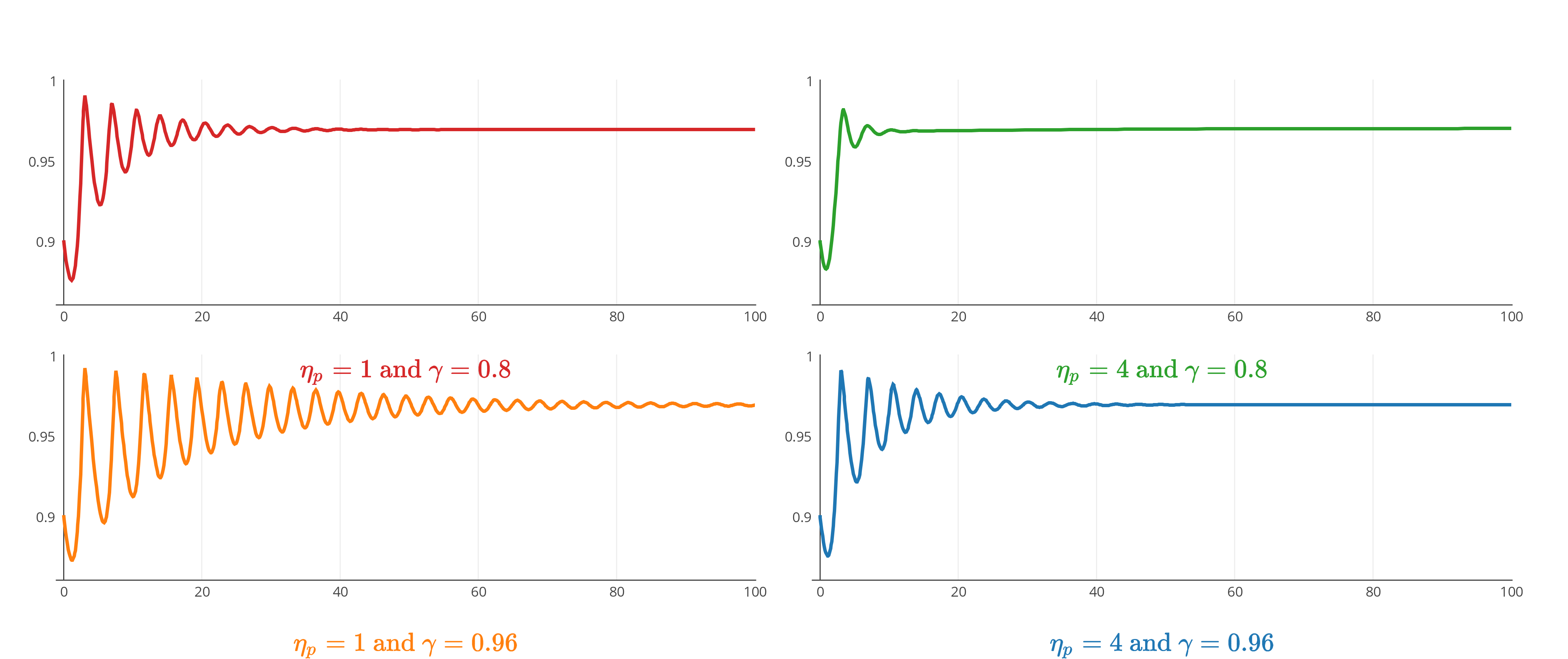
First it appears that $\eta_{p}$ and $(1-\gamma)$ have, as expected, a dampening effect on oscillations of the system. Recall that $\eta_{p}$ is the speed of adjustment of prices for a given wage share, whereas $\gamma$ is the proportion of inflation taken into consideration of wage negotiation. They also alter the value of the good equilibrium point. It is expected that the local basin of attraction is also affected, but this is not pursued here. Figure 1 below illustrates the dampening effect of $\eta_{p}$ and $(1-\gamma)$ on the oscillatory behavior of the employment rate $\lambda$.

Figure 1: Convergent trajectories for variable $\lambda(t)$ in system (26) with initial values $(\omega_{0},\lambda_{0},b_{0})=(0.9,0.9,0.3)$, and parameters defined in Section 5, except $(\eta_{p},\gamma)$.

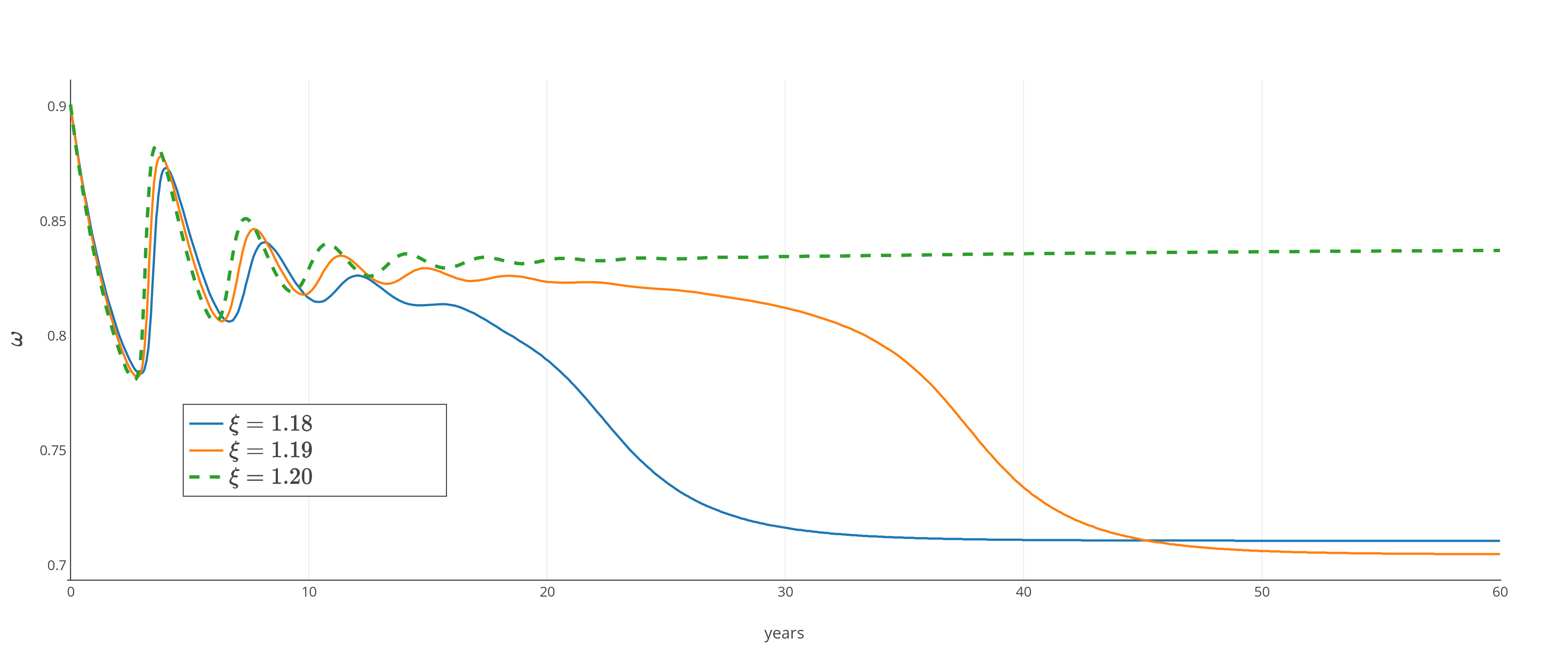
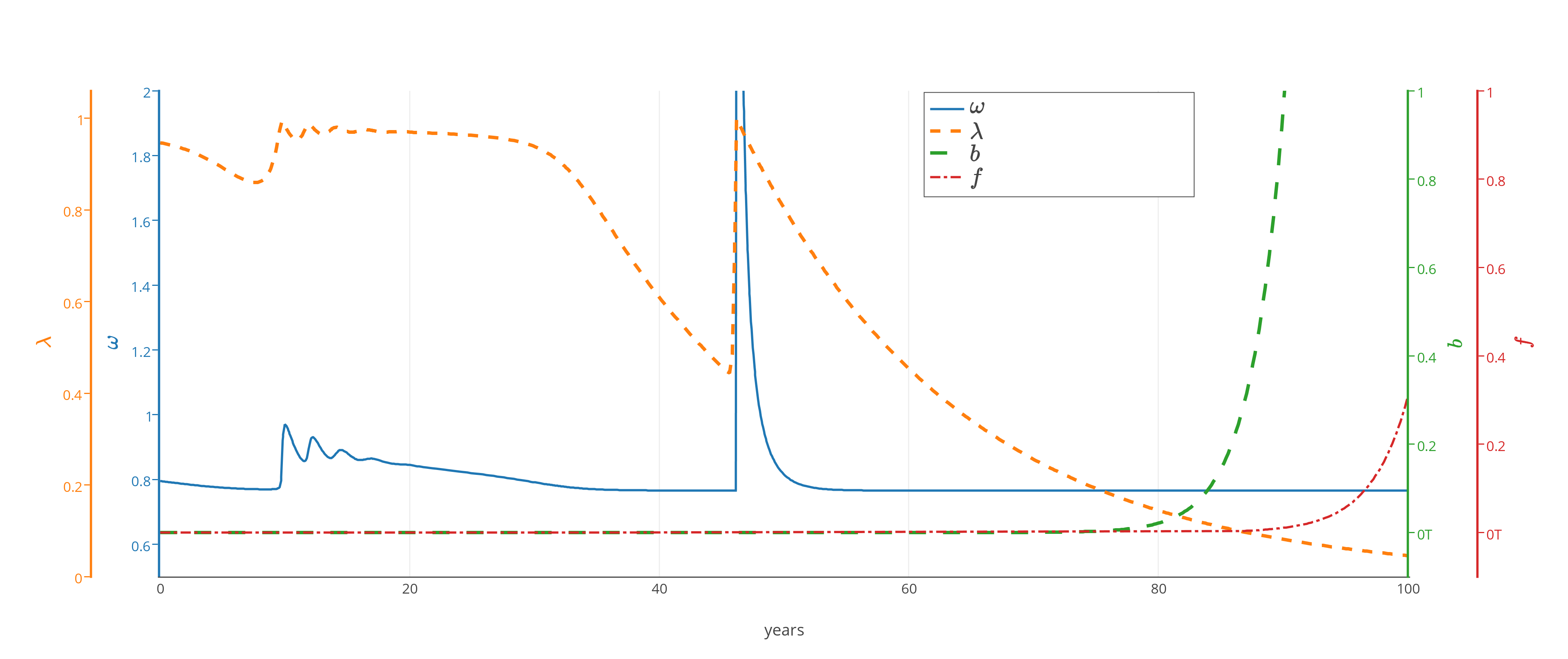
The parameter $\xi$ is even more influential. Its value crucially impacts condition (31), so that a slight decrease in the markup can lead to the absence of a good equilibrium point. This is illustrated by Figure 2, where a convergence toward the bad equilibrium $(\overline{\omega}_{3},0,+\infty)$ appears after dampened oscillations that first seem to converge to a good equilibrium.

Figure 2: Trajectories for variable $\omega(t)$ in system (26) with initial values $(\omega_{0},\lambda_{0},b_{0})=(0.9,0.9,0.3)$, and parameters defined in Section 5, except $\xi$.

The three-dimensional monetary Keen model (26) is then a privileged framework for studying the isolated effect of price parameters in comparison with the basic Keen model (14). While it exhibits new undesirable economic situations, it also shows accelerated convergence to equilibrium points, thus rendering the economic situation more stable, whether or not the result is considered good or bad.

5.2.2 Keen model with inflation and speculation

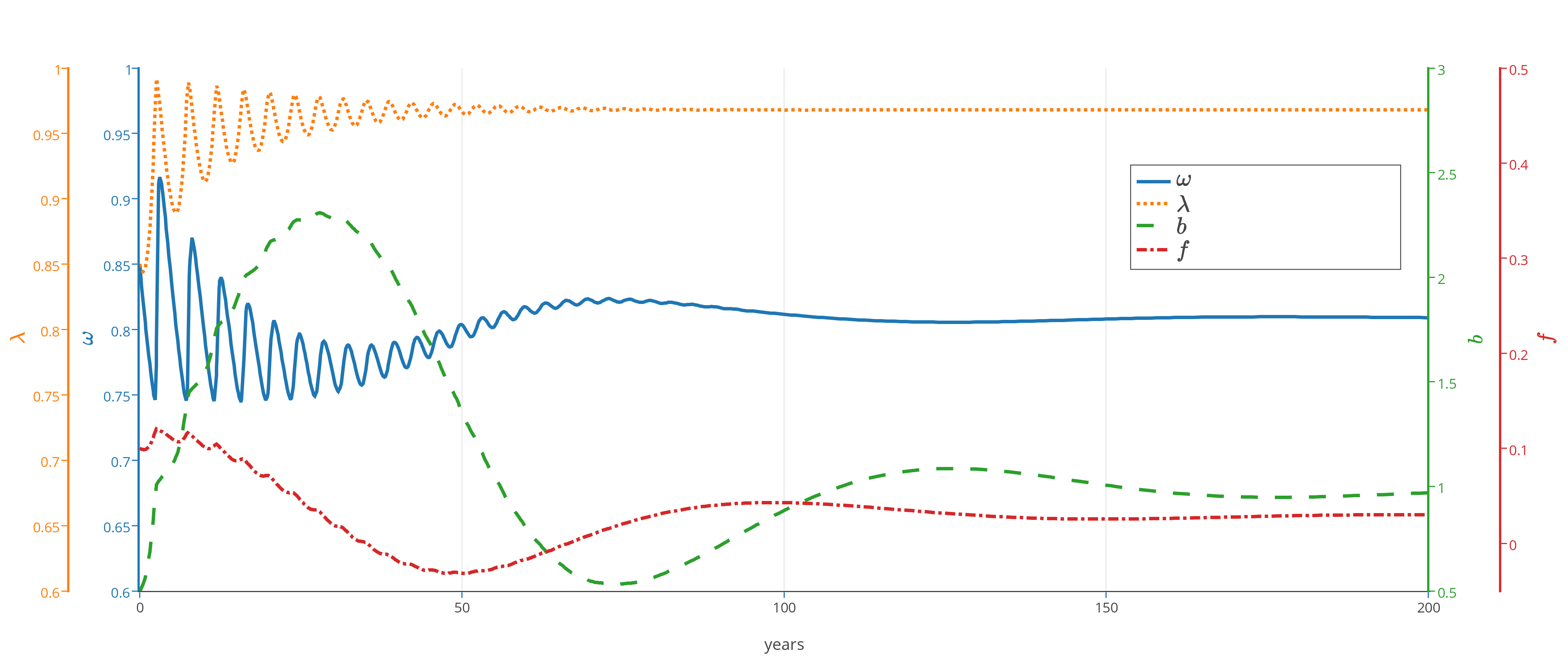
Similarly to the three-dimensional case, the higher the value of price parameters $\eta_{p}$ and $(1-\gamma)$, the faster the dampening of oscillations, when the economy converges to the good equilibrium $(\overline{\omega}_{1},\overline{\lambda}_{1},\overline{b}_{1},\overline{f}_{1})$. When we take low values for $\eta_{p}$ in particular, the case is very similar to the Keen model with speculation of [2], and Figure 3 pictures such a trajectory for system (51) with parameter $\eta_{p}=0.4$. One can then see two scales of oscillations due to different factors. The short-period oscillations are already present in system (14): they are given by the wage-employment variations, interpreted as business cycles in the Goodwin model, and dampened on the long run by the use of credit to compensate capital availability for work. The dampening speed is also highly influenced by the relaxation parameter $\eta_{p}$, which adjusts the price of capital and nominal growth to sustain wages requirements. The long-run variations are due to the adjustment of the financial flow $f$. The higher the parameter $\psi_{2}$, the shorter and the wider those fluctuations. This parameter represents the sensitivity of the flow $F$ to nominal growth output.

Figure 3: A convergent trajectory for system (51), $(\omega_{0},\lambda_{0},b_{0},f_{0})=(0.85,0.85,0.5,0.1)$, and parameters defined in Section 5.

Let us now come back to the initial parametrization (67), with $\eta_{p}=4$. The interest here is to analyze the effect of the speculation function $\Psi$, which is not explicit in the local stability analysis pursued in Section 4.2.1. The form of (71) implies that $\Psi>0$ if and only if $g(\pi)+i(\omega)>\psi_{1}$, so that this last term represent the threshold of speculation direction (in or out of financial markets).

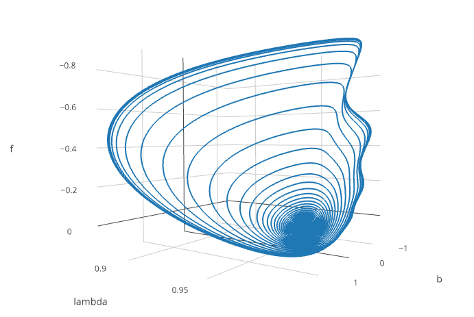
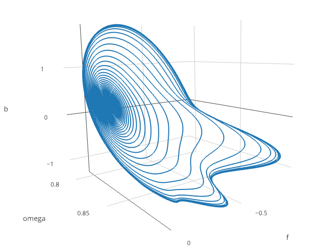
Depending on the value of the parameter $\psi_{1}$, the system exhibits either local stability of the good equilibrium or an absorbing limit cycle, provided that we start from a ”good” initial state $(\omega_{0},\lambda_{0},b_{0},f_{0})$. Even when the good equilibrium point (72) is still theoretically locally stable, its basin of attraction is very small. Starting numerically close to that good equilibrium, the trajectory actually converges on a very long term (+1000 years) to an elaborate limit cycle. Figure 4 illustrates such a claim.

Figure 4: A trajectory starting near the good equilibrium point and converging to a limit cycle. Left: projection in the phase subspace $(\lambda,b,f)$. Right: projection in the phase subspace $(\omega,b,f)$.

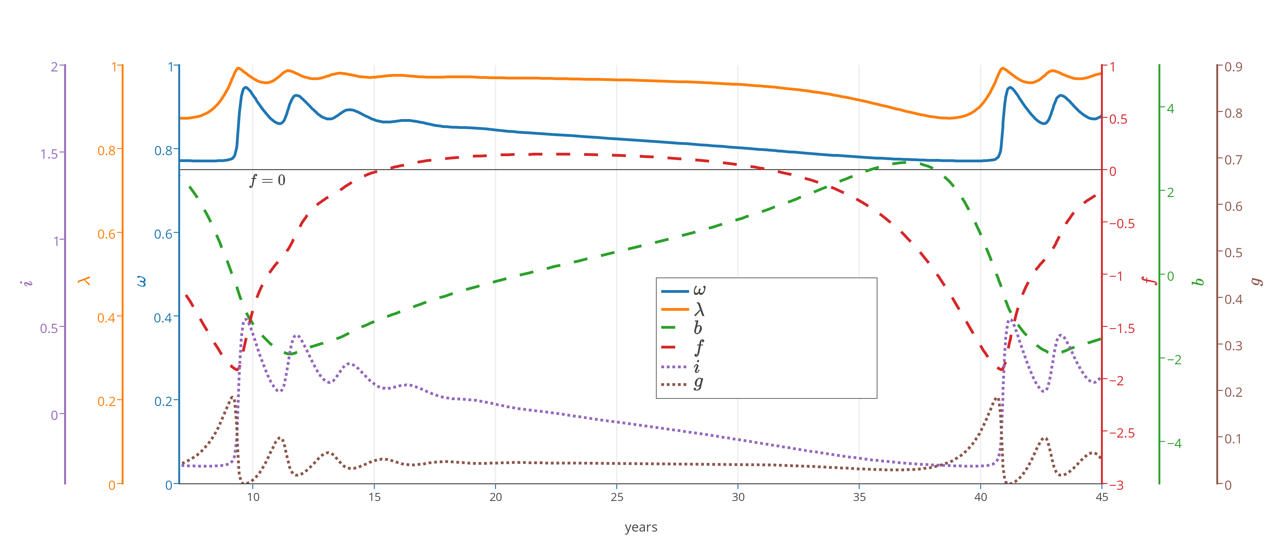
The limit cycle can be described as follows, with assistance of Figure 5. Starting the economy in a state of low debt (around years 9 and 10), it initially evolves with small cycles of oscillation between periods of high employment rate with high wage share, and periods with high profit share and low inflation rate. During this period, fluctuations in inflation and real growth cancel each other and the nominal growth has a steady, albeit slowly path. Speculation reacts accordingly and reduces its flow towards financial markets, directing it towards debt reduction instead. This in turn implies high profit rates, and pushes up the level of growth, as well as debt creation for investment purposes. The stability of growth above a certain threshold turns the financial flow back toward financial markets, increasing the debt level and debt service charge and stabilizing employment and speculation flow before year 20. The wage share steadily decreases together with inflation. Growth remains strong until year 30, sustained by credit creation. Nominal growth is however impacted by deflation, which reduces the flow of speculation into financial markets again. When the debt burden is too high, real investment decreases, reducing the output growth. At this point the speculative flow decreases sharply, and the debt burden decreases and allows for high profits again, high employment rate and in consequence, higher wages, around year 40.

If we reduce the value of $\psi_{1}$ in the above parameters configuration, then the speculation flow remains positive for smaller values of the nominal growth rate. There is no reversal of flow from speculative purposes back into debt repayment, and the debt service charges remain high. What happens is that a trajectory starting from the previous limit cycle then converges to the bad equilibrium $(\overline{\omega}_{3},0,+\infty,+\infty)$.

Figure 5: Description of the limit cycle over time for state variables $(\omega,\lambda,b,f)$, and auxiliary variables $(i,g)$.

Figure 6: A trajectory converging to the bad equilibrium $(\overline{\omega}_{3},0,+\infty,+\infty)$, starting from a point on the limit cycle of Figure 5.

References

- [1] Meghnad Desai. Growth cycles and inflation in a model of the class struggle. Journal of Economic Theory, 6(6):527–545, December 1973.
- [2] Matheus R. Grasselli and Bernardo Costa Lima. An analysis of the Keen model for credit expansion, asset price bubbles and financial fragility. Mathematics and Financial Economics, 6(3):191–210, 2012.
- [3] Matheus R. Grasselli and Adrien Nguyen Huu. Inventory dynamics in a debt-deflation model. In preparation, 2014.
- [4] Jon Hilsenrath and Brian Blackstone. Risk of deflation feeds global fears. Wall Street Journal, October 16, 2014.
- [5] Steve Keen. Finance and economic breakdown: Modeling Minsky’s “Financial Instability Hypothesis”. Journal of Post Keynesian Economics, 17(4):607–635, 1995.
- [6] Steve Keen. A monetary minsky model of the great moderation and the great recession. Journal of Economic Behavior and Organization, Doi 10.1016/j.jebo.2011.01.010:–, 2011.
- [7] Steve Keen. A monetary minsky model of the great moderation and the great recession. Journal of Economic Behavior and Organization, 86(0):221 – 235, 2013.
- [8] Joaquim Oliveira Martins, Stefano Scarpetta, and Dirk Pilat. Mark-up ratios in manufacturing industries: estimates for 14 oecd countries. Technical report, OECD Publishing, 1996.