Optimizing for an arbitrary perfect entangler: I. Functionals

Abstract

Optimal control theory is a powerful tool for improving figures of merit in quantum information tasks. Finding the solution to any optimal control problem via numerical optimization depends crucially on the choice of the optimization functional. Here, we derive a functional that targets the full set of two-qubit perfect entanglers, gates capable of creating a maximally-entangled state out of some initial product state. The functional depends on easily-computable local invariants and uniquely determines when a gate evolves into a perfect entangler. Optimization with our functional is most useful if the two-qubit dynamics allows for the implementation of more than one perfect entangler. We discuss the reachable set of perfect entanglers for a generic Hamiltonian that corresponds to several quantum information platforms of current interest.

I Introduction

Entanglement between quantum bits plays a fundamental role in quantum information processing. It can be generated between two qubits by suitable operations from the Lie group $SU(4)$. The geometric theory of $SU(4)$ formulated by Zhang et al. Zhang et al. (2003) provides a very useful classification of two-qubit operations in terms of their local equivalence classes. These are uniquely characterized by three real numbers known as local invariants Makhlin (2002). Each local equivalence class contains all the two-qubit gates which are equivalent up to single-qubit transformations and is characterized by a unique nonlocal content and thus has unique entangling capabilities.

The geometric theory has recently been combined with optimal control theory by Müller et al. Müller et al. (2011). Specifically, using the local invariants which uniquely characterize local equivalence classes, the optimization target was expanded from a specific unitary operation to the corresponding local equivalence class. This considerably relaxes the control constraints. The ensuing optimization algorithm Müller et al. (2011); Reich et al. (2012) allows for identifying those two-qubit gates out of a local equivalence class that can be implemented, for a given system Hamiltonian. The algorithm can be employed to determine the quantum speed limit Caneva et al. (2009), i.e., the fundamental limits for a given two-qubit system in terms of maximal fidelity and minimal gate time.

Here, we further explore the potential for quantum information processing offered by the combination of geometric theory and optimal control. Our starting point is the characterization of perfect entanglers provided by the geometric theory. Perfect entanglers (PEs) are nonlocal two-qubit operations that are capable of creating a maximally-entangled state out of some initial product state. In particular, we define a function to uniquely and easily identify whether a two-qubit operation is a PE. Since this function is given in terms of the local invariants, it can be easily incorporated into the optimal control functional used in Refs. Müller et al. (2011); Reich et al. (2012). This allows us to expand the optimization target to the full set of PEs, which corresponds to half of all local equivalence classes. The optimization functional may be thought of as measuring the “minimal distance” between the gate $U$ and the subset of matrices in $SU(4)$ which are PEs. It is zero for a PE and positive otherwise. The functional is remarkably easy to compute for any matrix, requiring only elementary algebra.

Optimization targeting the set of PEs will proceed along a path in the Weyl chamber, i.e., the reduced two-qubit parameter space, if the system dynamics allows for implementation of only a single local equivalence class containing a PE. However, our approach is most useful if more than one local equivalence class containing a PE can be reached. Optimization will then explore a larger portion of the Weyl chamber. We therefore also present an analysis of the reachable set of local equivalence classes, considering a generic two-qubit Hamiltonian that models superconducting qubits. The application of our optimization approach to examples is presented in the sequel to this paper.

This paper is organized as follows. The geometric theory is summarized in Section II with Section II.1 presenting a review of the way we decompose $SU(4)$ to separate the purely local operations from the ones which entangle two qubits, and Section II.2 reintroducing the set of easily-computable numbers which are invariant under the local operations. Section III describes the subspace of the entangling gates which are PEs and introduces the functional that indicates when we have realized a PE. The reachable set of PEs for a generic two-qubit Hamiltonian is discussed in Section IV. Section V concludes.

II Review of the geometric theory for two-qubit gates

II.1 Decomposition and Parametrization of $SU(4)$

All unitary gates operating on two-qubit states are described by a $4\times 4$ unitary matrix, an element of the compact Lie group $U(4)$. Any such matrix may be written as an element of $SU(4)$ multiplied by a number of modulus $1$, so the sixteen parameters we use to specify any gate are the phase of this $U(1)$-prefactor (an angle modulo $\pi/2$) and the fifteen real parameters of $SU(4)$.

Which fifteen parameters we choose are largely up to us; the ones we use in this work are those arising from the Cartan decomposition of the Lie algebra of the group, cf. Ref. Helgason (1978). This decomposition allows us to write any element of $SU(4)$ as a combination of two matrices in $SU(2)\otimes SU(2)$ and one in the maximal Abelian subgroup $\mathcal{A}=SU(4)/SU(2)\otimes SU(2)$.

The utility of this decomposition is apparent when we realise that, in the computational basis $\{\left|00\right\rangle,\left|01\right\rangle,\left|10\right\rangle,\left|11\right\rangle\}$, any operation which affects only the first qubit is represented by $U_{1}\otimes I$, and one affecting only the second is $I\otimes U_{2}$, where $U_{1}$ and $U_{2}$ are each $2\times 2$ unitary matrices. These local operations, which act separately and independently on the two qubits, are therefore described by matrices in $SU(2)\otimes SU(2)$. The operations which entangle the two qubits must then be entirely determined by the matrices from the Abelian subgroup $\mathcal{A}$. Gates are therefore denoted by equivalence classes living in $\mathcal{A}$; for example, [CNOT] is the set of gates which are equal to the CNOT gate up to local operations.

With all of this in hand, we choose the decomposition of $SU(4)$ such that our matrices take the form

$$U=k_{1}Ak_{2}\,,$$ (1)

where $k_{1}$ and $k_{2}$ are $4\times 4$ matrices in $SU(2)\otimes SU(2)$ and $A$ is in the maximal Abelian subgroup $\mathcal{A}$. Twelve of the fifteen coordinates necessary to specify any $SU(4)$ element are included in $k_{1}$ and $k_{2}$. Since we work with gates in $SU(4)$ modulo $SU(2)\otimes SU(2)$, we need only use the three coordinates $c_{1}$, $c_{2}$ and $c_{3}$ which parametrize the matrix $A$ through

$$A = \exp\left(-\frac{i}{2}\sum_{j=1}^{3}c_{j}\sigma_{j}\otimes\sigma_{j}\right)$$ (2)

$$= \prod_{j=1}^{3}\left[I\otimes I\cos\left(\frac{c_{j}}{2}\right)-i\sigma_{j}\otimes\sigma_{j}\sin\left(\frac{c_{j}}{2}\right)\right]\,,$$

where $\sigma_{x,y,z}$ are the usual Pauli matrices. (Later in this article we shall use the shorthand $\sigma_{i}^{(1)}=\sigma_{i}\otimes I$ and $\sigma_{i}^{(2)}=I\otimes\sigma_{i}$.) To ensure that each $U$ is given by a unique set of coordinates, we must restrict $c_{1}$, $c_{2}$ and $c_{3}$ to the Weyl chamber $W$ given by

$$0\leq c_{3}\leq c_{2}\leq c_{1}\leq\frac{\pi}{2}\quad\mbox{or}$$

$$\frac{\pi}{2}<c_{1}<\pi,\quad 0\leq c_{3}\leq c_{2}<\pi-c_{1}\,,$$

i.e., within the tetrahedron whose vertices are at $(0,0,0)$, $(\pi,0,0)$, $(\pi/2,\pi/2,0)$ and $(\pi/2,\pi/2,\pi/2)$ Zhang et al. (2003).

II.2 Local Invariants

Although $c_{1}$, $c_{2}$ and $c_{3}$ are defined in a straightforward manner, actually determining their values for a general element of $SU(4)$ can be difficult. Fortunately, there are three alternative parameters which can be used as coordinates for local equivalence classes on $\mathcal{A}$ which are far easier to obtain.

If we change from the standard computational basis $\{\left|00\right\rangle,\left|01\right\rangle,\left|10\right\rangle,\left|11\right\rangle\}$ to a Bell basis given by

$$\Bigg{\{}\frac{1}{\sqrt{2}}\left(\left|00\right\rangle-i\left|11\right\rangle\right) -\frac{1}{\sqrt{2}}\left(i\left|01\right\rangle-\left|10\right\rangle\right),$$ ,

$$\;-\frac{1}{\sqrt{2}}\left(i\left|01\right\rangle+\left|10\right\rangle\right) +\frac{1}{\sqrt{2}}\left(\left|00\right\rangle+i\left|11\right\rangle\right)\Bigg{\}},$$ ,

then our $SU(4)$ matrices become $U_{\mathrm{B}}=Q^{\dagger}UQ=Q^{\dagger}k_{1}Ak_{2}Q$, where

$$Q = \frac{1}{\sqrt{2}}\left(\begin{array}[]{cccc}1&0&0&i\\ 0&i&1&0\\ 0&i&-1&0\\ 1&0&0&-i\end{array}\right).$$

The eigenvalues of the matrix $m=U_{\mathrm{B}}^{\mathrm{T}}U_{\mathrm{B}}$ determine the local invariants of $U$ Makhlin (2002). The characteristic equation of $m$ is

$$\lambda^{4}-\mathrm{tr}(m)\lambda^{3}+\frac{1}{2}\left[\mathrm{tr}^{2}(m)-\mathrm{tr}\left(m^{2}\right)\right]\lambda^{2}-\mathrm{tr}^{*}(m)\lambda+1 = 0,$$

and so $\mathrm{tr}(m)$ and $\mathrm{tr}(m^{2})$ give the local invariants. These are complex numbers. Instead we may take as local invariants the three real numbers

$$g_{1} = \frac{1}{16}\mathrm{Re}\left\{\mathrm{tr}^{2}(m)\right\}\,,\,g_{2}=\frac{1}{16}\mathrm{Im}\left\{\mathrm{tr}^{2}(m)\right\}\,,$$

$$g_{3} = \frac{1}{4}\left[\mathrm{tr}^{2}(m)-\mathrm{tr}\left(m^{2}\right)\right]\,.$$

Since $m$, $m^{2}$ and their traces are readily computable using the simplest of matrix operations, values for $g_{1}$, $g_{2}$ and $g_{3}$ can be easily obtained for any $U\in SU(4)$.

Since $g_{1}$, $g_{2}$, $g_{3}$ are local invariants, they must be functions only of $c_{1}$, $c_{2}$ and $c_{3}$; some computation shows that they are, and have the explicit forms

$$g_{1} = \frac{1}{4}\big{[}\cos\left(2c_{1}\right)+\cos\left(2c_{2}\right)+\cos\left(2c_{3}\right)$$

$$+\cos\left(2c_{1}\right)\cos\left(2c_{2}\right)\cos\left(2c_{3}\right)\big{]}\,,$$

$$g_{2} = \frac{1}{4}\sin\left(2c_{1}\right)\sin\left(2c_{2}\right)\sin\left(2c_{3}\right)\,,$$

$$g_{3} = \cos\left(2c_{1}\right)+\cos\left(2c_{2}\right)+\cos\left(2c_{3}\right)\,.$$

These can be used to embed the tetrahedron defining the Weyl chamber into $g_{1}g_{2}g_{3}$-space; both spaces are shown in Figure 1, with cross-sections shown in Figure 2. The coordinates for the labeled points in both spaces are given in Table 1.

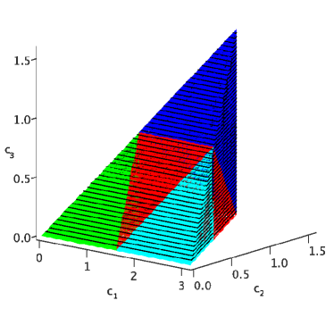
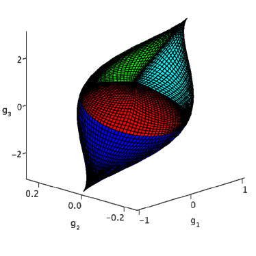
Figure 1: (Color online) The Weyl chamber in $c_{1}c_{2}c_{3}$ space (left) and its embedding in $g_{1}g_{2}g_{3}$ space (right). In both, $W_{0}$ is in green, $W_{0}^{*}$ in cyan, $W_{1}$ in blue and $W_{\mathrm{PE}}$ in red. (The contours shown are purely for illustrative purpose.)

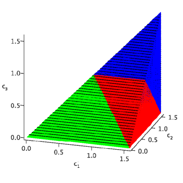
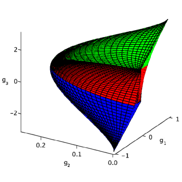
Figure 2: (Color online) The $0\leq c_{1}\leq\pi/2$ half of the Weyl chamber in $c_{1}c_{2}c_{3}$ space (left) and the corresponding $g_{2}\geq 0$ half in $g_{1}g_{2}g_{3}$ space (right). In both cases, the full chamber is obtained by reflection across the cross-section at the right of each figure.

point (gate)	$c_{1}$	$c_{2}$	$c_{3}$	$g_{1}$	$g_{2}$	$g_{3}$
$O$, $A_{1}$ ([$\openone$])	$0$, $\pi$	$0$	$0$	$1$	$0$	$3$
$A_{2}$ ([DCNOT])	$\pi/2$	$\pi/2$	$0$	$0$	$0$	$-1$
$A_{3}$ ([SWAP])	$\pi/2$	$\pi/2$	$\pi/2$	$-1$	$0$	$-3$
$B$ ([B-Gate])	$\pi/2$	$\pi/4$	$0$	$0$	$0$	$0$
$L$ ([CNOT])	$\pi/2$	$0$	$0$	$0$	$0$	$1$
$P$ ([$\sqrt{\mbox{SWAP}}$])	$\pi/4$	$\pi/4$	$\pi/4$	$0$	$1/4$	$0$
$Q$, $M$	$\pi/4$, $3\pi/4$	$\pi/4$	$0$	$1/4$	$0$	$1$
$N$	$3\pi/4$	$\pi/4$	$\pi/4$	$0$	$-1/4$	$0$
$R$	$\pi/2$	$\pi/4$	$\pi/4$	$-1/4$	$0$	$-1$

Table 1: The coordinates of selected points in the Weyl chamber (see Figures 1 and 2) in $c_{1}c_{2}c_{3}$ space and their corresponding local invariants.

A particular combination which is quite useful is $\sqrt{g_{1}^{2}+g_{2}^{2}}$; a quick calculation shows that

$$g_{1}^{2}+g_{2}^{2} = \frac{1}{16}\big{[}1+\cos\left(2c_{1}\right)\cos\left(2c_{2}\right)$$

$$+\cos\left(2c_{1}\right)\cos\left(2c_{3}\right)+\cos\left(2c_{2}\right)\cos\left(2c_{3}\right)\big{]}^{2}.$$

It is straightforward to confirm that the quantity inside the square brackets is always non-negative inside the Weyl chamber, so

$$\sqrt{g_{1}^{2}+g_{2}^{2}} = \frac{1}{4}\big{[}1+\cos\left(2c_{1}\right)\cos\left(2c_{2}\right)$$

$$+\cos\left(2c_{1}\right)\cos\left(2c_{3}\right)+\cos\left(2c_{2}\right)\cos\left(2c_{3}\right)\big{]}.$$

III A functional for perfect entanglers

The elements of $SU(4)$ which perfectly entangle two-qubit states all lie within the subset of the Weyl chamber $W$ bounded by the planes $c_{1}+c_{2}=\pi/2$, $c_{1}-c_{2}=\pi/2$ and $c_{2}+c_{3}=\pi/2$. This region is the 7-faced polyhedron with vertices at $(\pi/2,0,0)$, $(\pi/4,\pi/4,0)$, $(3\pi/4,\pi/4,0)$, $(\pi/2,\pi/2,0)$, $(\pi/4,\pi/4,\pi/4)$ and $(3\pi/4,\pi/4,\pi/4)$ Zhang et al. (2003). $W$ is thus divided up into four regions:

1. $W_{\mathrm{PE}}$, the perfect entanglers themselves.

2. $W_{0}$, the region between the origin (i.e., the identity element) and $W_{\mathrm{PE}}$, the tetrahedron bounded by (but not including) the wall $c_{1}+c_{2}=\pi/2$. All three local invariants are positive in this region.

3. $W_{0}^{*}$, between $(\pi,0,0)$ and $W_{\mathrm{PE}}$, bounded by $c_{1}-c_{2}=\pi/2$. In this region, $g_{1}$ and $g_{3}$ are positive and $g_{2}$ is negative. In fact, $W_{0}^{*}$ can be obtained from $W_{0}$ via the transformation $(g_{1},g_{2},g_{3})\rightarrow(g_{1},-g_{2},g_{3})$.

4. $W_{1}$, between $W_{\mathrm{PE}}$ and the [SWAP] gate at $(\pi/2,\pi/4,\pi/4)$, bounded by $c_{2}+c_{3}=\pi/2$. $g_{1}$ and $g_{3}$ are both negative and $g_{2}$ can have any sign.

One can construct functions based on a parametrization of $W_{PE}$ either in terms of $(c_{1},c_{2},c_{3})$ or in terms of $(g_{1},g_{2},g_{3})$. In the following, we will refer to $(c_{1},c_{2},c_{3})$ as the Weyl coordinates and to $(g_{1},g_{2},g_{3})$ as the local invariants or Makhlin coordinates.

III.1 Gate fidelity for perfect entanglers in terms of the Weyl coordinates $c_{1}$, $c_{2}$, $c_{3}$

In order to define a fidelity for an arbitrary perfect entangler in terms of the Weyl coordinates $c_{1}$, $c_{2}$, $c_{3}$, we generalize the notion of the gate fidelity for a specific desired gate $V$,

$$F = \frac{1}{4}\left|\mathrm{tr}\left(U^{\dagger}V\right)\right|\,,$$

where $U$ is the actually-implemented gate, and we assume $U\in SU(4)$. Allowing for complete freedom in the local transformations, this becomes

$$F = \max_{k_{1},k_{2}\in SU(2)\otimes SU(2)}\frac{1}{4}\mathrm{Re}\left\{\mathrm{tr}\left(U^{\dagger}k_{1}Vk_{2}\right)\right\}\,,$$

where we have substituted the modulus by the real part implying that without loss of generality we can choose the global phase of the local transformations such that the trace is real. The maximum over all local transformations $k_{1}$, $k_{2}$ is difficult to evaluate. However, the local transformations can be chosen such that $U$ and $V$ are given by their canonical forms $A_{U}=\exp[-i/2\sum_{j}c_{j}^{U}\sigma_{j}\sigma_{j}]$ and $A_{V}=\exp[-i/2\sum_{j}c_{j}^{V}\sigma_{j}\sigma_{j}]$. We denote this choice by $k_{i}=k_{i,U}k_{i,V}$. It can be shown that the partial derivatives of $F$ with respect to the $k_{i}$ vanish and that $F=1$ for $U=V$. The latter simply follows from equality of the Weyl coordinates. The partial derivatives are obtained by parametrizing the $k_{i}$ as elements of $SU(2)\otimes SU(2)$ and the canonical forms of the non-local parts by $c_{1}$, $c_{2}$, $c_{3}$. This choice of the local transformations yields

$$F = \frac{1}{4}\mathrm{Re}\left\{\mathrm{tr}\left(U^{\dagger}k_{1,U}k_{1,V}^{\dagger}Vk_{2,V}^{\dagger}k_{2,U}\right)\right\}$$

$$= \frac{1}{4}\mathrm{Re}\left\{\mathrm{tr}\left(A_{U}^{\dagger}A_{V}\right)\right\}$$

$$= \frac{1}{4}\mathrm{Re}\left\{\mathrm{tr}\left(Q^{\dagger}A_{U}^{\dagger}QQ^{\dagger}A_{V}Q\right)\right\}$$

$$= \frac{1}{4}\mathrm{Re}\left\{\mathrm{tr}\left(F_{U}^{\dagger}F_{V}\right)\right\}$$

with

$$F_{U} = Q^{\dagger}A_{U}Q$$

$$= \mathrm{diag}(\mathrm{e}^{\imath\frac{c_{1}-c_{2}+c_{3}}{2}},\mathrm{e}^{\imath\frac{c_{1}+c_{2}-c_{3}}{2}},\mathrm{e}^{\imath\frac{-c_{1}-c_{2}-c_{3}}{2}},\mathrm{e}^{\imath\frac{-c_{1}+c_{2}+c_{3}}{2}})$$

$$= \mathrm{diag}(\mathrm{e}^{\imath\phi_{1,U}},\mathrm{e}^{\imath\phi_{2,U}},\mathrm{e}^{\imath\phi_{3,U}},\mathrm{e}^{\imath\phi_{4,U}})\,$$

and $F_{V}=Q^{\dagger}A_{V}Q$, respectively. Inserting the explicit forms of $F_{U}$ and $F_{V}$, we obtain

$$F = \frac{1}{4}\mathrm{Re}\left\{\mathrm{tr}\left(F_{U}^{\dagger}F_{V}\right)\right\}$$ (4)

$$= \frac{1}{4}\sum_{j=1}^{4}\cos(\varphi_{j,U}-\varphi_{j,V})$$

$$= \frac{1}{4}\bigg{(}\cos\frac{\Delta c_{1}-\Delta c_{2}+\Delta c_{3}}{2}+\cos\frac{\Delta c_{1}+\Delta c_{2}-\Delta c_{3}}{2}$$

$$+\cos\frac{\Delta c_{1}+\Delta c_{2}+\Delta c_{3}}{2}+\cos\frac{\Delta c_{1}-\Delta c_{2}-\Delta c_{3}}{2}\bigg{)}$$

$$= \cos\frac{\Delta c_{1}}{2}\cos\frac{\Delta c_{2}}{2}\cos\frac{\Delta c_{3}}{2}\approx 1-\frac{|\Delta\vec{c}|^{2}}{8}\,,$$

where $\Delta c_{i}=c_{U,i}-c_{V,i}$. In order to find the closest perfect entangler $V$ for a given gate $U$, we have to maximize the fidelity given by Eq. (4) with respect to $c_{V,i}$. To this end, we can exploit that the sectors $W_{0}$, $W_{0}^{*}$, $W_{1}$ are separated from the polyhedron $W_{PE}$ by three planes, and $U$ is a perfect entangler if and only if

$$c_{1}+c_{2}\geq\frac{\pi}{2}\mbox{, }c_{1}-c_{2}\leq\frac{\pi}{2} c_{2}+c_{3}\leq\frac{\pi}{2}\,.$$ and

If $U$ lies in the polyhedron of perfect entanglers we can simply choose $V=U$ and arrive at perfect fidelity $F=1$. If $U\in W_{0}$, we have $c_{1}+c_{2}\leq\frac{\pi}{2}$, and the closest perfect entangler both in terms of fidelity and distance of the Weyl coordinates is given by the projection of $U$ onto the wall, i.e., $c_{V,1}=\frac{\pi}{4}+\frac{c_{U,1}-c_{U,2}}{2}$, $c_{V,2}=\frac{\pi}{4}+\frac{c_{U,2}-c_{U,1}}{2}$, and $c_{V,3}=c_{U,3}$. The distance vector between $U$ and $V$ as a function of the Weyl coordinates is then given by

$$\Delta\vec{c} = \left(\frac{c_{U,1}+c_{U,2}}{2}-\frac{\pi}{4},\frac{c_{U,1}+c_{U,2}}{2}-\frac{\pi}{4},0\right)\,.$$

With the analogous approach for $W_{0}^{*}$ and $W_{1}$ and using Eq. (4), we arrive at

$$F_{PE}(U)=\begin{cases}\cos^{2}\frac{c_{U,1}+c_{U,2}-\frac{\pi}{2}}{4}\,,\qquad c_{1}+c_{2}\leq\frac{\pi}{2}\\ \cos^{2}\frac{c_{U,2}+c_{U,3}-\frac{\pi}{2}}{4}\,,\qquad c_{2}+c_{3}\geq\frac{\pi}{2}\\ \cos^{2}\frac{c_{U,1}-c_{U,2}-\frac{\pi}{2}}{4}\,,\qquad c_{1}-c_{2}\geq\frac{\pi}{2}\\ 1\qquad\qquad\text{otherwise (inside $W_{PE}$).}\end{cases}$$

As desired, this fidelity is a function of $c_{U,i}$; it equals one if and only if $U$ is a perfect entangler and is smaller than 1 otherwise. $F_{PE}(U)$ can be used for optimization if no analytic gradients with respect to the states are needed.

Often the dynamics may explore a Hilbert space that is larger than the logical subspace of the qubits. The evolution in the logical subspace may then correspond to a non-unitary gate $\tilde{U}$. Employing a singular value decomposition of $\tilde{U}$ and renormalizing the singular values, a unitary approximation $U$ of $\tilde{U}$ is obtained analogously to the unitary case. This allows to utilize the same ideas that have lead to the fidelity $F_{PE}$ defined above. The gate fidelity $F$ becomes

$$F = \frac{1}{4}\left|\mathrm{tr}\left(\tilde{U}^{\dagger}V\right)\right|\,,$$

where $V=k_{1,U}A_{V}k_{2,U}$ and $A_{V}$ is the canonical form of the perfect entangler closest to the unitary approximation $U$, as measured by the distance in Weyl coordinates. In order to avoid explicit calculation of the $k_{i,U}$ (which would have to be done in every iteration step of an optimization algorithm), we find the lower bound on the fidelity,

$$F = \frac{1}{4}\left|\mathrm{tr}\left(\tilde{U}^{\dagger}V\right)\right|=\frac{1}{4}\mathrm{Re}\left\{\mathrm{tr}\left(\tilde{U}^{\dagger}V\right)\right\}$$

$$= \frac{1}{4}\mathrm{Re}\left\{\mathrm{tr}\left(U^{\dagger}V\right)\right\}+\frac{1}{4}\mathrm{Re}\left\{\mathrm{tr}\left((\tilde{U}-U)^{\dagger}V\right)\right\}$$

$$\geq \frac{1}{4}\mathrm{Re}\left\{\mathrm{tr}\left(U^{\dagger}V\right)\right\}-\left|\frac{1}{4}\mathrm{tr}\left((\tilde{U}-U)^{\dagger}V\right)\right|$$

$$\geq F_{PE}(U)-||\tilde{U}-U||\,,$$

where we have first used the choice of $V$ that makes the trace real, and then used both the Cauchy-Schwarz inequality and $||V||=1$.

III.2 Perfect entanglers and the local invariants

For optimization algorithms that utilize gradient information it is necessary to express the functional in a way that allows for analytic expressions of the derivatives Reich et al. (2012). This is not the case if the functional is expressed in terms of the Weyl coordinates $(c_{1},c_{2},c_{3})$ Müller et al. (2011). We therefore seek to express the boundaries of the polyhedron $W_{PE}$ in terms of the local invariants $(g_{1},g_{2},g_{3})$.

Let us first look at the boundary with $W_{0}$: it is defined by the plane $c_{1}+c_{2}=\pi/2$, and along this wall, $\cos(2c_{2})=-\cos(2c_{1})$ and $\sin(2c_{2})=\sin(2c_{1})$. This means that the values of the local invariants on this wall depend only on $c_{1}$ and $c_{3}$ through

$$g_{1} = \frac{1}{4}\sin^{2}\left(2c_{1}\right)\cos\left(2c_{3}\right),$$

$$\sqrt{g_{1}^{2}+g_{2}^{2}} = \frac{1}{4}\sin^{2}\left(2c_{1}\right),$$

$$g_{3} = \cos\left(2c_{3}\right).$$

We can eliminate $c_{1}$ and $c_{3}$ entirely from the above to give

$$g_{3} = \left\{\begin{array}[]{cl}\frac{g_{1}}{\sqrt{g_{1}^{2}+g_{2}^{2}}}&g_{1}\neq 0\mbox{ or }g_{2}\neq 0,\\ 1&g_{1}=g_{2}=0\end{array}\right.$$

as the equation defining the PE boundary in terms of the local invariants. If we repeat this analysis for the walls separating $W_{0}^{*}$ and $W_{1}$ from $W_{\mathrm{PE}}$, we find that the same equation describes them all. So any $U$ lying precisely on the boundary of $W_{\mathrm{PE}}$ has local invariants satisfying $g_{3}=g_{1}/\sqrt{g_{1}^{2}+g_{2}^{2}}$.

This suggests the definition of a function $d$ which depends on an $SU(4)$ matrix $U$ via its local invariants and vanishes on the boundary of $W_{\mathrm{PE}}$:

$$d\left(g_{1},g_{2},g_{3}\right) = g_{3}\sqrt{g_{1}^{2}+g_{2}^{2}}-g_{1}\,.$$ (6)

This is not the only combination of the local invariants which vanishes on the boundary of $W_{\mathrm{PE}}$; the reason we choose this particular definition of $d$ comes from the fact that it is continuous for all values of $g_{1}$, $g_{2}$ and $g_{3}$. When we rewrite it in terms of the Weyl coordinates, we obtain the particularly simple form

$$d = \frac{1}{4}\left[\cos\left(2c_{1}\right)+\cos\left(2c_{2}\right)\right]\left[\cos\left(2c_{1}\right)+\cos\left(2c_{3}\right)\right]$$

$$\times\left[\cos\left(2c_{2}\right)+\cos\left(2c_{3}\right)\right].$$

It is this form which allows us to see immediately that $d$ is manifestly positive in $W_{0}$; thus, in terms of the local invariants, all points in $W_{0}$ satisfy $g_{3}\sqrt{g_{1}^{2}+g_{2}^{2}}-g_{1}>0$. We noted above that $W_{0}^{*}$ is simply the mirror-reflection of $W_{0}$, since we may obtain it by changing the sign of $g_{2}$; thus, in reality, $W_{0}$ and $W_{0}^{*}$ are not disconnected in terms of the local invariants, but are joined along the $g_{2}=0$ plane. This is seen explicitly in Figure 1, where $W_{0}\cup W_{0}^{*}$ consists of the green and cyan regions of the Weyl chamber.

In $g$-space, the boundary separating $W_{0}\cup W_{0}^{*}$ from $W_{\mathrm{PE}}$ is a single continuous surface. To be precise, if we use cylindrical coordinates $(\rho,\phi,z)$ defined by $g_{1}=\rho\cos\phi$, $g_{2}=\rho\sin\phi$ and $g_{3}=z$, the boundary is given by the surface

$$z=\cos\phi -\frac{\pi}{2}\leq\phi\leq\frac{\pi}{2},\,\frac{1}{4}\sin^{2}\phi\leq\rho\leq\frac{1}{4}.$$ with

The part of this wall adjoining $W_{0}$ is the yellow surface illustrated in Figure 3.

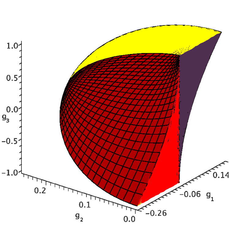
Figure 3: The $g_{2}\geq 0$ half of the set of perfect entanglers $W_{\mathrm{PE}}$ in $g_{1}g_{2}g_{3}$ space. This space is divided into three regions: the red volume, where $d>0$; the violet volume, where $d<0$; and the surface composed of the boundary between them and the uppermost (yellow) and lowermost (obscured) surfaces, where $d=0$.

As a result, if optimization starts from a gate $U$ in $W_{0}\cup W_{0}^{*}$, then $d(g_{1},g_{2},g_{3})=g_{3}\sqrt{g_{1}^{2}+g_{2}^{2}}-g_{1}$ is an optimization function to reach a PE gate: we know that $d>0$ for the initial gate and it reaches zero at the boundary with $W_{\mathrm{PE}}$. However, $d$ vanishes elsewhere as well: not only on the boundary between $W_{\mathrm{PE}}$ and $W_{1}$, but everywhere on the surface $z=\cos\phi$. This surface is comprised not only of the boundaries that $W_{\mathrm{PE}}$ has with $W_{1}$ and $W_{0}\cup W_{0}^{*}$ but also the boundary between the red and violet regions in Figure 3. However, this surface lies entirely within $W_{\mathrm{PE}}$, so the only gates $U$ for which $d(g_{1},g_{2},g_{3})$ vanishes are perfect entanglers.

However, $d$ alone cannot tell us if we continue into the interior of $W_{\mathrm{PE}}$. If $U$ happens to cross the curve $z=\cos\phi$, $\rho=\sin^{2}\phi/4$, then either $d(g_{1},g_{2},g_{3})$ becomes positive and we have a PE, or it becomes negative and we are in $W_{1}$ and do not have a PE. In either of these two cases, the value of $d$ alone will not be a good enough indicator of whether we have evolved to a PE; further information might be necessary.

III.3 An optimization functional for perfect entanglers

The discussion of the previous two sections motivates our formulation of a functional $\mathcal{D}(U)$ that provides a definitive answer as to whether or not an $SU(4)$ gate $U$ is locally equivalent to a perfect entangler. That is, the functional vanishes if $U$ is a perfect entangler and is positive otherwise.

The functional $\mathcal{D}(U)$ is based on the function $d(g_{1},g_{2},g_{3})$ but also takes into account in which sector of the Weyl chamber – $W_{0}$, $W_{0}^{*}$, $W_{1}$ or $W_{\mathrm{PE}}$ – the local equivalence class of the gate $U$ is located. Its construction is presented below:

1. Compute the three Makhlin invariants $g_{1}$, $g_{2}$ and $g_{3}$ for $U$ as usual.

2. Next, find the three roots $z_{1}$, $z_{2}$ and $z_{3}$ of the cubic equation

   $$~{}~{}~{}~{}~{}~{}z^{3}-g_{3}z^{2}+\left(4\sqrt{g_{1}^{2}+g_{2}^{2}}-1\right)z+\left(g_{3}-4g_{1}\right)=0$$

   ordered such that $-1\leq z_{1}\leq z_{2}\leq z_{3}\leq 1$. These roots – which are functions of $g_{1}$, $g_{2}$ and $g_{3}$ – facilitate the inverse map $\left(g_{1},g_{2},g_{3}\right)\rightarrow\left(c_{1},c_{2},c_{3}\right)$ and thus provide the location of the gate within the $c$-space Weyl chamber Watts et al. (2013).
   

3. Define $d$ as in Eq. (6) and $s$ as

   $$s\left(g_{1},g_{2},g_{3}\right) := \pi-\cos^{-1}z_{1}-\cos^{-1}z_{3}$$

   The definition of the functional $\mathcal{D}$ depends on the signs of these two functions:

   1. If $d$ and $s$ are both positive, then

      $$\mathcal{D}(U) = g_{3}\sqrt{g_{1}^{2}+g_{2}^{2}}-g_{1}.$$

   2. If $d$ and $s$ are both negative, then

      $$\mathcal{D}(U) = g_{1}-g_{3}\sqrt{g_{1}^{2}+g_{2}^{2}}.$$

   3. In any other case,

      $$\mathcal{D}(U) = 0.$$

This gives the desired functional, one that is zero when the two-qubit gate is a perfect entangler and positive otherwise. Its evaluation requires only the Makhlin invariants and a way of finding the largest and smallest roots of a cubic equation. The functional is also differentiable and straightforward to implement within the framework of optimal control.

IV Controllability in the Weyl chamber

Optimization towards an arbitrary perfect entangler is most meaningful if the system dynamics allows the polyhedron of perfect entanglers to be approached from more than one direction or, more generally, for optimization paths in the Weyl chamber that explore more than one dimension. We therefore investigate the corresponding requirements on a generic two-qubit Hamiltonian,

$$H[u_{1}(t),u_{2}(t)] = \sum_{\alpha=1,2}\frac{\omega_{\alpha}}{2}\sigma_{z}^{(\alpha)}+u_{1}(t)\left(\sigma_{x}^{(1)}+\lambda\sigma_{x}^{(2)}\right)$$ (7)

$$+u_{2}(t)\left(\sigma_{x}^{(1)}\sigma_{x}^{(2)}+\sigma_{y}^{(1)}\sigma_{y}^{(2)}\right)\,.$$

Here, $\sigma_{i}^{(\alpha)}$ is the $i^{\mathrm{th}}$ Pauli operator acting on the $\alpha^{\mathrm{th}}$ qubit of transition frequency $\omega_{\alpha}$, $u_{1}(t)$ the single-qubit control field, where $\lambda$ describes how strongly $u_{1}(t)$ couples to the second qubit relative to the first one, and $u_{2}(t)$ is the two-qubit interaction control field. As discussed in the sequel to this paper, Eq. (7) is used to model qubits realized with superconducting circuits.

We analyze the solutions to the differential equation

$$\dot{U}\left(t\right)=-iH\left[u\left(t\right)\right]U\left(t\right),\quad U\left(0\right)=\openone\,$$ (8)

for the unitary transformations $U$ generated by the Hamiltonian (7). The reachable set of unitary transformations for a Hamiltonian is given in terms of the corresponding dynamical Lie algebra. It can be generated by taking the terms in (7) as a basis (neglecting orthonormalization for simplicity),

$$\sigma_{z}^{(1)}\,,\,\sigma_{z}^{(2)}\,,\,\sigma_{x}^{(1)}+\lambda\sigma_{x}^{(2)}\,,\,\sigma_{x}^{(1)}\sigma_{x}^{(2)}+\sigma_{y}^{(1)}\sigma_{y}^{(2)}\,,$$

and constructing the repeated Lie brackets of these operators. This quickly yields all 15 canonical basis operators of $SU(4)$, consisting of the single-qubit operators $\sigma_{x}^{(1)}$, $\sigma_{x}^{(2)}$, $\sigma_{y}^{(1)}$, $\sigma_{y}^{(2)}$, $\sigma_{z}^{(1)}$, and $\sigma_{z}^{(2)}$, as well as the entangling operators $\sigma_{x}^{(1)}\sigma_{y}^{(2)}$, $\sigma_{y}^{(1)}\sigma_{x}^{(2)}$, $\sigma_{y}^{(1)}\sigma_{z}^{(2)}$, $\sigma_{z}^{(1)}\sigma_{y}^{(2)}$, $\sigma_{x}^{(1)}\sigma_{z}^{(2)}$, $\sigma_{z}^{(1)}\sigma_{x}^{(2)}$, $\sigma_{x}^{(1)}\sigma_{x}^{(2)}$, $\sigma_{y}^{(1)}\sigma_{y}^{(2)}$, and $\sigma_{z}^{(1)}\sigma_{z}^{(2)}$. Hence the system is completely controllable, and any point in the Weyl chamber can be reached.

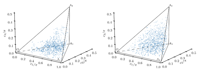
Figure 4: (Color online) Sampling of reachable points in the Weyl chamber, obtained by solving Eq. (8) for the Hamiltonian (7) ($\lambda=1$), a random pulse $u_{1}(t)\in[0,1]$, constant $u_{2}(t)\equiv 10^{-3}$, and 1000 time steps. On the left, result for $\omega_{1}=1.0\neq\omega_{2}=1.1$, providing the full set of 15 generators in the Lie algebra. On the right, result for $\omega_{1}=\omega_{2}=1$, providing 9 generators. In both cases, every point in the Weyl chamber can be reached.

The complete controllability can be verified numerically, by solving Eq. (8) for a random sequence of pulse values. The resulting gates are shown in the left of Fig. 4, and demonstrate full controllability, since there are points in all regions of the Weyl chamber. Continuing the procedure to infinity would eventually fill the entire chamber. Neither setting $u_{2}(t)$ constant nor choosing $\lambda=0$ places any restrictions on the controllability – indeed it is sufficient if either the single qubit terms or the interaction term is controllable. While the controllability in this example was analyzed for arbitrary values of the parameters, the form of the Hamiltonian and the ratio between $\omega_{1,2}$ and $u_{2}$ fits the description of superconducting transmon qubits, with qubit energies in the GHz range and static qubit-qubit-coupling in the MHz range.

Introducing symmetries in the Hamiltonian (7) reduces the controllability. First, we consider a situation in which the two qubits operate at the same frequency $\omega_{1}=\omega_{2}$. In this case, the dynamic Lie algebra consists of only 9 instead of 15 operators. Consequently, not every two-qubit gate can be implemented. However, the nine operators include $\sigma_{x}^{(1)}\sigma_{x}^{(2)}$, $\sigma_{y}^{(1)}\sigma_{y}^{(2)}$, $\sigma_{z}^{(1)}\sigma_{z}^{(2)}$, which are sufficient to reach every point in the Weyl chamber, cf. Eq. (2). This is illustrated on the right of Fig. 4. Despite the reduced controllability, the Weyl chamber is more evenly filled after the same 1000 propagation steps as on the left. This counterintuitive finding is due to the lower dimension of the random walk, with no resources being “wasted” on the missing six single-qubit directions.

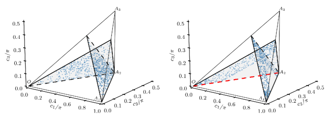
Figure 5: (Color online) Same as Fig. 4 for the fully degenerate case $\omega_{1}=\omega_{2}=0$ and two random pulses $u_{1}(t),u_{2}(t)\in[0,1]$. Not every point in the Weyl chamber can be reached. For independent pulses $u_{1}(t)$, $u_{2}(t)$ (left), the dynamic Lie algebra consists of four generators, and a two-dimensional subset of the Weyl chamber can be reached, indicated by the shaded triangles, $O$–$(\frac{2\pi}{3},\frac{\pi}{3},\frac{\pi}{3})$–$A_{2}$ and $A_{1}$–$(\frac{\pi}{3},\frac{\pi}{3},\frac{\pi}{3})$–$A_{2}$. The reachable set is further reduced to a subset if $u_{1}(t)\equiv u_{2}(t)$ (right), i.e., the single-qubit and interaction operators couple to the same pulse. Lastly, without single-qubit driving ($u_{1}(t)\equiv 0$), only a one-dimensional subset of the Weyl chamber can be reached, the red line $O$–$A_{2}$.

The set of gates that can be implemented with Hamiltonian (7) is more severely restricted if both qubits are completely degenerate, $\omega_{1}=\omega_{2}=0$. This is typical for superconducting charge qubits operated at the “charge degeneracy point”. Without any drift term, the Lie algebra consists of only four generators, $\sigma_{z}^{(1)}\sigma_{y}^{(2)}+\sigma_{y}^{(1)}\sigma_{z}^{(2)}$ and $\sigma_{y}^{(1)}\sigma_{y}^{(2)}-\sigma_{z}^{(1)}\sigma_{z}^{(2)}$ in addition to the two original terms. The implications for controllability in the Weyl chamber are not immediately obvious since three generators can be sufficient to obtain full Weyl chamber controllability. The easiest approach is to perform a numerical analysis, the results of which are shown on the left of Fig. 5. Two independent randomized pulses $u_{1}(t)$ and $u_{2}(t)$ were used. The reachable points lie on a plane, which due to the reflection symmetries appears as two triangular branches. Note that almost none of the common two-qubit gates are included in this set.

If only a single pulse is available to drive both the single-qubit and two-qubit terms, $u_{1}(t)\equiv u_{2}(t)$, and the qubits are degenerate, $\omega_{1}=\omega_{2}=0$, there is a single generator for the dynamics. This situation is shown on the right of Fig. 5. Although there is only a single generator for the dynamics, a two-dimensional subset of the Weyl chamber can be reached. However, the subset is no longer the full plane as it is for two independent pulses (left of Fig. 5). Without single-qubit control, the center of the plane is not longer reachable. It is important to remember that while a single generator yields points on a line in the Weyl chamber (not necessarily a straight one), it can still fill an arbitrary subset of the Weyl chamber, due to reflections at the boundaries. A similar example, restricted to the ground plane of the Weyl chamber, has been analyzed in Ref. Zhang et al. (2003).

Lastly, if there is no control over the individual qubits at all, $u_{1}(t)\equiv 0$, the only remaining generator is $\sigma_{x}^{(1)}\sigma_{x}^{(2)}+\sigma_{y}^{(1)}\sigma_{y}^{(2)}$. This corresponds to the straight line $O$–$A_{2}$ in the Weyl chamber, shown in red in Fig. 5. The line is reflected back onto itself at the $A_{2}$ point. Thus, in this case only a truly one-dimensional subset of reachable gates in the Weyl chamber can be realized.

For a Hamiltonian that allows for a one-dimensional search-space only, optimal control calculations with a functional targeting all perfect entanglers will not yield results better than direct gate optimization. In contrast, for Hamiltonians allowing for two or three search directions in the Weyl chamber, cf. Figures 4 and 5, the polyhedron of perfect entanglers may be approached from several different angles. Optimization with a functional targeting all perfect entanglers is then non-trivial. In such a search, the optimized solution will depend on additional constraints in the functional and the initial guess field. This will be explored in the sequel to this paper.

V Summary

We have revisited the parametrization of two-qubit gates, i.e., elements of the Lie group $SU(4)$, in terms of three real numbers, the local invariants Zhang et al. (2003), in order to derive an optimization functional for optimal control to target the whole subset of perfectly entangling two-qubit gates. We first identified an analytical function of the local invariants $d(g_{1},g_{2},g_{3})$ which becomes zero at the boundary of the subset of perfect entanglers but can be of any sign within this subset. We rectified this ambiguity by using $d(g_{1},g_{2},g_{3})$ to obtain a functional $\mathcal{D}(U)$ that determines definitively if we are within the set of perfect entanglers. Specifically, $\mathcal{D}(U)$ yields zero if a two-qubit gate $U$ is a perfect entangler and is positive otherwise.

This functional represents a generalization of our earlier work on optimizing for a local equivalence class Müller et al. (2011) instead of a specific gate Palao and Kosloff (2003). Optimization with such a functional is useful if one wants to implement an arbitrary perfect entangler. In this case, a functional targeting the whole subset of perfect entanglers allows for more flexibility and thus potentially better control than optimization for a specific gate or a single local equivalence class. Furthermore, since gates locally equivalent to perfect entanglers occupy nearly 85% of $SU(4)$ Watts et al. (2013); Musz et al. (2013), the target of such a functional is very large indeed.

The full potential of such a generalized search strategy can, however, only be utilized if the Hamiltonian is sufficiently complex, allowing to approach the subset of perfect entanglers from more than one direction. For a generic two-qubit Hamiltonian, we have therefore analyzed the basic requirements for a nontrivial search. Not surprisingly, symmetries in the Hamiltonian preclude a full Weyl chamber search. Caution is necessary in particular when operating in the regime of the rotating-wave approximation which typically introduces degeneracies and compromises complete controllability.

The sequel to this paper illustrates optimization with the perfect entanglers’ functional for several numerical examples. The physical models, when restricted to the logical subspace, correspond to the generic Hamiltonian analyzed here.

References

• Zhang et al. (2003) J. Zhang, J. Vala, S. Sastry, and K. B. Whaley, Phys. Rev. A 67, 042313 (2003).
• Makhlin (2002) Y. Makhlin, Quant. Inf. Proc. 1, 243 (2002).
• Müller et al. (2011) M. M. Müller, D. M. Reich, M. Murphy, H. Yuan, J. Vala, K. B. Whaley, T. Calarco, and C. P. Koch, Phys. Rev. A 84, 042315 (2011).
• Reich et al. (2012) D. M. Reich, M. Ndong, and C. P. Koch, J. Chem. Phys. 136, 104103 (2012).
• Caneva et al. (2009) T. Caneva, M. Murphy, T. Calarco, R. Fazio, S. Montangero, V. Giovannetti, and G. E. Santoro, Phys. Rev. Lett. 103, 240501 (2009).
• Helgason (1978) S. Helgason, Differential geometry, Lie groups, and symmetric spaces (Academic, New York, 1978).
• Blais et al. (2007) A. Blais, J. Gambetta, A. Wallraff, D. I. Schuster, S. M. Girvin, M. H. Devoret, and R. J. Schoelkopf, Phys. Rev. A 75, 032329 (2007).
• Palao and Kosloff (2003) J. P. Palao and R. Kosloff, Phys. Rev. A 68, 062308 (2003).
• Watts et al. (2013) P. Watts, M. O’Connor, and J. Vala, Entropy 15, 1963 (2013).
• Musz et al. (2013) M. Musz, M. Kuś, and K. Życzkowski, Phys. Rev. A 87, 022111 (2013).