Transport Theory of Metallic B20 Helimagnets

Abstract

B20 compounds are a class of cubic helimagnets harboring nontrivial spin textures such as spin helices and skyrmions. It has been well understood that the Dzyaloshinskii-Moriya (DM) interaction is the origin of these textures, and the physics behind the DM interaction is the spin-orbital coupling (SOC). However the SOC shows its effect not only on the spins, but also on the electrons. In this paper, we will discuss effects of the SOC on the electron and spin transports in B20 compounds. An effective Hamiltonian is presented from symmetry analysis, and the spin-orbital coupling therein shows anomalous behaviors in anisotropic magnetoresistance (AMR) and helical resistance. New effects such as inverse spin-galvanic effect is proposed, and the origin of the DM interaction is discussed.

I Introduction

Symmetry is a central topic of modern physics and material science. Reduced symmetry has given rise to innumerable novel phenomena. For example, breaking of the translational symmetry leads to the emergence of lattices and crystals, which are the platforms of condensed matter studies. The highest symmetry of a lattice has the point group of $O_{h}$, where most of the ferromagnetic materials belong to. Surprises have been brought by further reducing this symmetry. B20 compound, with representatives of FeSiSchlesinger et al. (1993); DiTusa et al. (1997), MnSiPfleiderer et al. (2004); Mühlbauer et al. (2009); Ritz et al. (2013) , FeGeYu et al. (2011); Huang and Chien (2012), and Cu₂SeO₃Seki et al. (2012), is such an interesting class of materials. Although B20 compound has a cubic lattice, it has the lowest symmetry in this crystal system. Complicated distributions of atoms dramatically bring down the symmetry, where inversion, mirror, or four-fold rotational symmetries are absent. Abundant phenomena are emerging consequently, among which the most attractive one is the presence of nontrivial spin textures like helices and skyrmions.

Spin helix is a spatially modulated magnetic texture. It is present in magnetic materials with competing interactions. It has been observed in B20 family Fe_1-xCo_xSi by real-space imagingUchida et al. (2006). In this case, the Dzyaloshinskii-Moriya (DM) interactionDzyaloshinsky (1958); Moriya (1960)

$$H_{\text{DM}}=\mathbf{D}\cdot({\bf S}_{i}\times{\bf S}_{j})$$ (1)

between neighboring spins plays an important role. Broken inversion symmetry in B20 compounds is the physical origin of this interaction. Under an inversion operation about the center of the joint line, two neighboring spins are exchanged, and the DM interaction flips sign due to its cross product nature. In contrast, the Heisenberg exchange, $H_{\text{H}}=-J{\bf S}_{i}\cdot{\bf S}_{j}$ is unchanged under this operation, thus respects the inversion symmetry. The Heisenberg exchange tends to align neighboring spins, while the DM interaction tends to form an angle of $\pi/2$. As a result of the competition, a finite angle is expanded by these two spins, whose successive arrangement generates the spin helix. Spin helix is not the only result of breaking inversion symmetry, but also the magnetic skyrmionSkyrme (1961); Rö\ssler et al. (2006); Mühlbauer et al. (2009); Yu et al. (2010), a topological spin texture. It is stabilized in B20 compounds at finite magnetic fields and temperatures.

In the light of nontrivial spin modulation in helix and promising spintronics applications of the skyrmion, a throughout understanding of the electron and spin transports in B20 compounds is an urgent subject. Longitudinal magnetoresistance measurements have been performed to map out the phase diagrams containing helical and skyrmion phasesKadowaki et al. (1982); Du et al. (2014). On the other hand, due to the emergent electromagnetismZang et al. (2011); Schulz et al. (2012), skyrmion phase can be precisely determined by the Hall measurementsNeubauer et al. (2009); Lee et al. (2009); Kanazawa et al. (2011); Huang and Chien (2012); Li et al. (2013). A peculiar non-Fermi liquid behavior is also addressed in MnSi single crystalsPfleiderer et al. (2004); Ritz et al. (2013), which is intimately related to the topology of spin texturesWatanabe et al. (2014). However, a deep study of the spin transports in B20 compounds still lacks. Recently, an experiment on anisotropic magnetoresistance (AMR) is performed in bulk samples of Fe_1-xCo_xSiHuang et al. (2014a). It is surprisingly observed that compared to usual AMR in cobalt or other cubic ferromagnetic materials, the magnetoresistance shows two, instead of four, peaks. It shows that the system lacks of the four-fold rotational symmetry, which is compatible with the reduced symmetry in B20 compounds. However the microscopic origin waits to be revealed. In another experiment, the measurement on helical resistance shows an ultra-low resistance ratio of $1.35$ with current parallel and perpendicular to the helixHuang et al. (2014b). It has predicted theoretically and well tested experimentally that this ratio should be larger than $3$. This observation apparently violate this common concept.

These two experiments suggest a new mechanism involving nontrivial spin scatterings, and thus inevitably call for the important effects of the spin-orbital coupling (SOC) on the conduction electrons in B20 compounds. The SOC has already shows its power in the spin interactions in B20 compounds. It is well known that a nonvanishing DM interaction requires not only the inversion symmetry breaking, but also a large SOCMoriya (1960). However effects of the SOC on conduction electrons have never been discussed. In this paper, we will show that the SOC well explains the two experiments above, and provides several other proposals.

This paper is organized as follows. In the following section, an effective Hamiltonian is constructed, where both linear and cubic SOC terms are present. Section III shows that these SOC terms are the microscopic origin of the DM interactions in B20 compounds. In section IV and V, the linear SOC gives rise to inverse spin-galvanic effect and ultra-low ratio of helical resistance, respectively. In section VI, the importance of the cubic SOC is revealed, which provides the microscopic mechanism of the anomalous AMR effect.

II Effective Hamiltonian

In order to understand the transport behaviors of B20 compounds, the first priority is to construct the effective Hamiltonian of the conduction electrons. As we are interested in the long-range behaviors, only momenta around the $\Gamma$ point will be relevant. The bands around other high symmetry points in the Brillouin zone might cross the Fermi energy, and contribute to the transports in some form. However, the qualitative behavior, especially the symmetries, will not change.

The importance of the SOC indicates that the conventional quadratic dispersion, $H({\bf k})=\hbar^{2}{\bf k}^{2}/2m$, is not adequate in understanding the spin-related transports. Therefore, additional terms coupling spin and momentum is called for. To this end, we analyze the symmetry of the B20 compounds and employ the theory of invariants to construct the effective HamiltonianWinkler (2003).

In the international notation, the space group of B20 compounds is $P_{2_{1}3}$, where $2$ and $3$ mean the two-fold and three-fold rotational symmetries respectively, while $1$ indicates a fractal translation in the space group operation. No other symmetries are present. Around the $\Gamma$ point, the fractal rotation does not change the space group irreducible representationsDresselhaus et al. (2010), thus is not relevant, and the space group is isomorphic to its K-group, which is a group containing all the point group operations within the space group. Irreducible representations of the space group at $\Gamma$ point is the same as that of the K-group. For $P_{2_{1}3}$, the K-group is the $T23$ group, containing 12 elements; 1 identity, 3 $C_{2}$ rotations ($\pi$ rotations about axis [100], [010], and [001], and 8 $C_{3}$ rotations (Clockwise rotations of $2\pi/3$ about directions [$\pm$1,$\pm$1,$\pm$1]). Compared to the complete group operations in the $O_{h}$ group, four-fold rotations, inversions, and mirror symmetries are absent.

Once spin is taken into account, a $2\pi$ rotation in the spin space reverses the sign, and should be treated as an additional group operation. One thus has to consider the double group of $T23$, whose irreducible representations and characters are listed in Tab. (1). Operations with bars are joint action of point group element and the $2\pi$ spin rotation.

Table 1: The character table for the double group of $T23$.

$T23$	$E$	$\bar{E}$	$4C_{3}$	$4\bar{C}_{3}$	$3C_{2}+3\bar{C}_{2}$	$4C_{3}^{-1}$	$4\bar{C}_{3}^{-1}$
$\Gamma_{1}$	1	1	1	1	1	1	1
$\Gamma_{2}$	1	1	$w$	$w$	1	$w^{2}$	$w^{2}$
$\Gamma_{3}$	1	1	$w^{2}$	$w^{2}$	1	$w$	$w$
$\Gamma_{4}$	3	3	0	0	-1	0	0
$\Gamma_{5}$	2	-2	1	-1	0	1	-1
$\Gamma_{6}$	2	-2	$w$	$-w$	0	$w^{2}$	$-w^{2}$
$\Gamma_{7}$	2	-2	$w^{2}$	$-w^{2}$	0	$w$	$-w$

First principle calculations on metallic B20 materials, such as MnSi and FeGe, show that the orbitals around the Fermi surface are mainly d-orbitalsJeong and Pickett (2004). Under spin-orbit coupling, these orbitals are split into $j=5/2$ and $j=3/2$ orbitals, which correspond to $D_{5/2}$ and $D_{3/2}$ irreducible representations of the rotation group respectively. The character of a rotation of angle $\alpha$ in $D_{j}$ is given by

$$\chi=\frac{\sin((j+\frac{1}{2})\alpha)}{\sin(\frac{1}{2}\alpha)}$$ (2)

In the crystal field, these orbitals are further split into suborbitals, which corresponds to the decomposition in terms of $T23$’s irreducible representations;

$$D_{5/2}\downarrow T=\Gamma_{5}\oplus\Gamma_{6}\oplus\Gamma_{7}$$ (3)

$$D_{3/2}\downarrow T=\Gamma_{6}\oplus\Gamma_{7}$$ (4)

In reality, all these suborbitals might be relevant around the Fermi surface. In addition, there are four magnetic atoms in each unit cell, leading to a total of 20 bands. In order to capture the key feature of these materials, we would like to keep the Hamiltonian in the minimal form. Only one band out of three representations $\Gamma_{5,6,7}$ will be considered. The resulting Hamiltonian will be two by two, the simplest Hamiltonian taking into account the SOC.

The model Hamiltonian $H$ communicating the Hilbert spaces corresponding to irreducible representations $\alpha$ and $\beta$ is in general

$$H(\mathbf{k})=\sum_{l_{1}^{\alpha}=1}^{n_{\alpha}}\sum_{l_{2}^{\beta}=1}^{n_{\beta}}h(\mathbf{k})|l_{1}^{\alpha}\rangle\langle l_{2}^{\beta}|$$ (5)

Here $n_{\alpha}$ and $n_{\beta}$ are dimensions of these two representations respectively. In the current case, band mixing is neglected such that $\alpha=\beta$. $l_{1}^{\alpha}$ labels the basis in the irreducible representation $\alpha$. The operator part $|l_{1}^{\alpha}\rangle\langle l_{2}^{\beta}|$ transforms as the product representation $\Gamma_{\alpha}^{\ast}\times\Gamma_{\beta}$, which can be decomposed as the direct sum of irreducible representations $\Gamma_{\alpha}^{\ast}\times\Gamma_{\beta}=\oplus_{\gamma}\Gamma_{\gamma}$. The basis $X_{l_{3}^{\gamma}}^{\gamma}$ of an irreducible representation $\Gamma_{\gamma}$ contained in this product representation is the superposition of direct products $|l_{1}^{\alpha}\rangle\langle l_{2}^{\beta}|$ as $X_{l_{3}^{\gamma}}^{\gamma}=\sum_{l_{1}^{\alpha}=1}^{n_{\alpha}}\sum_{l_{2}^{\beta}=1}^{n_{\beta}}C_{l_{1}^{\alpha}l_{2}^{\beta},l_{3}^{\gamma}}^{\alpha\beta,\gamma}|l_{1}^{\alpha}\rangle\langle l_{2}^{\beta}|$, where $C_{l_{1}^{\alpha}l_{2}^{\beta},l_{3}^{\gamma}}^{\alpha\beta,\gamma}$ are the Clebsh-Gordan coefficientsKoster (1957). To keep the Hamiltonian invariant under group operations, $h(\mathbf{k})$ must be an irreducible tensor operator in the representation $\Gamma_{\gamma}^{\ast}$, such that $H(\mathbf{k})$ belongs to the trivial representation $\Gamma_{1}$ contained in the product representation $\Gamma_{\gamma}^{\ast}\times\Gamma_{\gamma}$. As a consequence, the invariant Hamiltonian is given by

$$H(\mathbf{k}) = \sum_{\gamma}^{\alpha\beta}a_{\gamma}^{\alpha\beta}\sum_{1}^{n_{\gamma}}h_{l_{3}^{\gamma}}^{\gamma}(\mathbf{k})X_{l_{3}^{\gamma}}^{\gamma}$$

$$= \sum_{\gamma}^{\alpha\beta}a_{\gamma}^{\alpha\beta}\sum_{1}^{n_{\gamma}}h_{l_{3}^{\gamma}}^{\gamma}(\mathbf{k})\left(\sum_{l_{1}^{\alpha}=1}^{n_{\alpha}}\sum_{l_{2}^{\beta}=1}^{n_{\beta}}C_{l_{1}^{\alpha}l_{2}^{\beta},l_{3}^{\gamma}}^{\alpha\beta,\gamma}|l_{1}^{\alpha}\rangle\langle l_{2}^{\beta}|\right)$$

where coefficients $a_{\gamma}^{\alpha\beta}$ are free parameters that cannot be dictated from the symmetry analysis.

For $\Gamma_{5}$, $\Gamma_{5}^{\ast}\times\Gamma_{5}=\Gamma_{1}\oplus\Gamma_{4}$. However $X_{1}^{\Gamma_{1}}$ and all the three matrices $X_{1,2,3}^{\Gamma_{4}}$ are all trivial identity matrices. Therefore the effective can be reduced to be spinless, and spin-orbital coupling is absent. The corresponding Hamiltonian is therefore the simplest quadratic one $H({\bf k})=\hbar^{2}{\bf k}^{2}/2m$, which does not bring anything new. New physics comes when we turn to $\Gamma_{6}$ or $\Gamma_{7}$ representations. As these two representations are complex conjugate to each other, the effective Hamiltonians are the same. In the following, we will take $\Gamma_{6}$ for example without loss of generality.

$$\Gamma_{6}^{\ast}\times\Gamma_{6}=\Gamma_{1}\oplus\Gamma_{4}$$ (8)

$$X_{1}^{\Gamma_{1}} = \left(\begin{array}[]{cc}\text{ \ }1\text{ \ }&0\\ 0&\text{ \ }1\text{ \ }\end{array}\right)\text{, }X_{1}^{\Gamma_{4}}=\left(\begin{array}[]{cc}0&-i/\sqrt{3}\\ -i/\sqrt{3}&0\end{array}\right)$$ (13)

$$X_{2}^{\Gamma_{4}} = \left(\begin{array}[]{cc}0&1/\sqrt{3}\\ -1/\sqrt{3}&0\end{array}\right)\text{, }X_{3}^{\Gamma_{4}}=\left(\begin{array}[]{cc}-i/\sqrt{3}&0\\ 0&i/\sqrt{3}\end{array}\right)$$ (18)

It shows explicitly that $X_{i}^{\Gamma_{4}}=-i/\sqrt{3}\sigma_{i}\,$, where $\sigma_{i}$ are three Pauli matrices. The overall factor -$i/\sqrt{3}$ can be absorbed into the factor $a_{\gamma}^{\alpha\beta}$ in Eq. (LABEL:eq:HamiltonianGroup). Now the remaining job is to construct the irreducible tensor operators $h_{l_{3}^{\gamma}}^{\gamma}(\mathbf{k})$. For $\Gamma_{1}$, it is very simple that $h_{1}^{\Gamma_{1}}(\mathbf{k})=\mathbf{k}^{2}/2m$. While for $\Gamma_{4}$, two basis may apply. $h_{i}^{\Gamma_{4}}(\mathbf{k})=(k_{x},k_{y},k_{z})$, or $h_{i}^{\Gamma_{4}}=(k_{x}(k_{y}^{2}-k_{z}^{2}),k_{y}(k_{z}^{2}-k_{x}^{2}),k_{z}(k_{x}^{2}-k_{y}^{2}))$, which are on the first and third orders in momentum ${\bf k}$ respectively. Terms of second order in ${\bf k}$ break the time reversal symmetry once coupled to the spin, thus can be neglected. As a consequence, the effective Hamiltonian for conduction electrons in B20 compounds is given by

$$H = \frac{\mathbf{k}^{2}}{2m}+\alpha(k_{x}\sigma_{x}+k_{y}\sigma_{y}+k_{z}\sigma_{z})$$

$$+ \beta[k_{x}\sigma_{x}(k_{y}^{2}-k_{z}^{2})+k_{y}\sigma_{y}(k_{z}^{2}-k_{x}^{2})+k_{z}\sigma_{z}(k_{x}^{2}-k_{y}^{2})]$$

This Hamiltonian can also be intuitively guessed from simple symmetry analysis. The presence of $C_{3}$ symmetry enforces the permutation symmetry in the Hamiltonian, while the $C_{2}$ symmetry rules out most of the combinations. It is worth emphasizing that the linear spin-orbital coupling ${\bf k}\cdot\boldsymbol{\sigma}$ is not adequate, as it is a full rotational symmetric term. $C_{4}$ symmetry is also respected by this term, but is apparently broken in $T23$ group. It is the cubic spin-orbital coupling, the last term in Eq. (LABEL:fullHamiltonian), that breaks $C_{4}$. Therefore Eq. (LABEL:fullHamiltonian) is the minimal Hamiltonian that faithfully describes the symmetry of B20 compounds.

The cubic spin-orbital coupling is well known in III-V semiconductors induced by bulk inversion asymmetry (BIA) Žutić et al. (2004). The linear term ${\bf k}\cdot\boldsymbol{\sigma}$ is a new term. It will be discussed in the following that it captures most of the nontrivial physics in B20 compounds. As $\boldsymbol{\sigma}$ is a pseudo-vector, ${\bf k}\cdot\boldsymbol{\sigma}$ is a pseudo-scalar. This is thus a forbidden term in lattices with any inversion or mirror symmetries. That is why it is absent in the III-V semiconductors and most of the ferromagnetic materials. However, elements in the $T23$ point group are only pure rotations, so that ${\bf k}\cdot\boldsymbol{\sigma}$ is allowed, and contributes significantly to the long range behaviors.

III Origin of Spin Interactions

Real space images of B20 compounds have shown that the spin helix therein looks like a successive array of Bloch wallsUchida et al. (2006), where magnetizations are rotating in a plane perpendicular to their propagation direction. In addition, the skyrmion has a double twist structureYu et al. (2010). These features are well described by the DM interaction in the following shape

$$H_{DM}=D\hat{r}_{ij}\cdot({\bf S}_{i}\times{\bf S}_{j}),$$ (21)

namely the DM vector $\mathbf{D}$ in Eq. (1) should point from one spin to the other. Although it is compatible with the symmetry Leonov (2014), the microscopic origin still lacks. However, it can be understood by the SOC in our effective Hamiltonian as follows.

Quantitatively, we can employ the field approach to calculate the Ruderman-Kittel-Kasuya-Yosida (RKKY) interaction between two neighboring spins ${\bf S}_{1}$ and ${\bf S}_{2}$Ruderman and Kittel (1954); Kasuya (1956); Yosida (1957). The electron’s action is given by

$$S = \sum_{n}\int d^{3}\mathbf{k}\bar{\psi}(-\mathbf{k},-i\omega_{n})(-i\omega_{n}+\frac{\mathbf{k}^{2}}{2m}+\alpha\mathbf{k\cdot\sigma})\psi(\mathbf{k},i\omega_{n})$$

$$+\sum_{i=1}^{2}\sum_{n}\int d^{3}\mathbf{k}\bar{\psi}(-\mathbf{k-q},-i\omega_{n})\mathbf{S}_{i}\cdot\mathbf{\sigma}\text{e}^{-i\mathbf{q}\cdot\mathbf{R}_{i}}\psi(\mathbf{k},i\omega_{n})$$

where $\mathbf{R}_{i}$ are the positions of two spins. The spin interaction can be derived by integrating out the electrons using the gradient expansion. Up to the second order, the spin-spin interaction is given by

$$S_{\text{eff}}=-2\sum_{n}\int d^{3}\mathbf{k}Tr[G({\bf R},i\omega_{n})\mathbf{S}_{1}\cdot\mathbf{\sigma}G(-{\bf R},i\omega_{n})\mathbf{S}_{2}\cdot\mathbf{\sigma}]$$ (23)

where $\mathbf{R}=\mathbf{R}_{1}-\mathbf{R}_{2}$, and $G({\bf R},i\omega_{n})$ is the real-space Green’s function defined as

$$G({\bf R},i\omega_{n}) = \int d^{3}\mathbf{k}\frac{\text{e}^{-i\mathbf{k}\cdot\mathbf{R}}}{-i\omega_{n}+\frac{\mathbf{k}^{2}}{2m}-\alpha\mathbf{k\cdot\sigma}}$$

$$= \int_{0}^{\infty}dk\int_{0}^{\pi}d\theta k^{2}\sin\theta$$

$$\times\int_{0}^{2\pi}d\varphi\frac{i\omega_{n}-\frac{k^{2}}{2m}+\alpha\mathbf{k\cdot\sigma}}{(-i\omega_{n}+\frac{k^{2}}{2m})^{2}-\alpha^{2}k^{2}}\text{e}^{-i\mathbf{k}\cdot\mathbf{R}}$$

One can decompose the momentum $\mathbf{k}$ into directions parallel with and perpendicular to $\hat{R}$ as ${\bf k}=({\bf k}\cdot\hat{R})\hat{R}+(\hat{R}\times{\bf k})\times\hat{R}\equiv{\bf k}_{\parallel}+{\bf k}_{\perp}$. Apparently, because of ${\bf k}_{\perp}\cdot\mathbf{R}=0$, $\exp(i{\bf k}_{\perp}\cdot{\bf R})=1$, and

$$\int_{0}^{2\pi}d\varphi\frac{\alpha\mathbf{k}_{\perp}\mathbf{\cdot\sigma}}{(-i\omega_{n}+\frac{k^{2}}{2m})^{2}-\alpha^{2}k^{2}}=0.$$ (26)

The Only contribution comes from the coupling between ${\bf k}_{\parallel}$ and Pauli matrices. Thus

$$G({\bf R},i\omega_{n}) = \int_{0}^{\infty}dk\int_{0}^{\pi}d\theta k^{2}\sin\theta$$ (27)

$$\times\int_{0}^{2\pi}d\varphi\frac{i\omega_{n}-\frac{k^{2}}{2m}+\alpha\mathbf{k}_{\parallel}\mathbf{\cdot\sigma}}{(-i\omega_{n}+\frac{k^{2}}{2m})^{2}-\alpha^{2}k^{2}}\text{e}^{-i\mathbf{k}_{\parallel}\cdot\mathbf{R}}$$

$$= 2\pi\int_{0}^{\infty}dk\int_{0}^{\pi}d\theta k^{2}\sin\theta$$

$$\times\frac{i\omega_{n}-\frac{k^{2}}{2m}+\alpha k\cos\theta\hat{R}\mathbf{\cdot\sigma}}{(-i\omega_{n}+\frac{k^{2}}{2m})^{2}-\alpha^{2}k^{2}}\text{e}^{-ikR\cos\theta}$$

$$\equiv G_{0}(R)+G_{1}(R){\bf R}\cdot\boldsymbol{\sigma}$$

where

$$G_{0}(R)=2\pi\int_{0}^{\infty}dk\int_{0}^{\pi}d\theta\frac{k^{2}\sin\theta(i\omega_{n}-\frac{k^{2}}{2m})}{(-i\omega_{n}+\frac{k^{2}}{2m})^{2}-\alpha^{2}k^{2}}\text{e}^{-ikR\cos\theta}$$ (28)

and

$$G_{1}(R)=\frac{2\pi}{R}\int_{0}^{\infty}dk\int_{0}^{\pi}d\theta\frac{\alpha k^{3}\sin\theta\cos\theta}{(-i\omega_{n}+\frac{k^{2}}{2m})^{2}-\alpha^{2}k^{2}}\text{e}^{-ikR\cos\theta}$$ (29)

One can easily get these Green’s functions by evaluating contour integrals. The real part of the poles of $k$ gives rise to the Friedel oscillations.

Consequently, the effective RKKY Hamiltonian is given by

$$H^{\text{RKKY}}=-\frac{2}{\beta}\sum_{n}[(G_{0}^{2}+G_{1}^{2})\mathbf{S}_{1}\cdot\mathbf{S}_{2}+2G_{0}G_{1}\mathbf{R}\cdot(\mathbf{S}_{1}\times\mathbf{S}_{2})]$$ (30)

The first term in the Heisenberg exchange, while the second term is the DM interaction. Compared to Eq. (1), the DM vector $\mathbf{D}$ is along ${\bf R}={\bf R}_{1}-{\bf R}_{2}$, which is consistent with Eq. (21) for B20 compounds. One can easily show that even the cubic spin orbital coupling in Eq. (LABEL:fullHamiltonian) is included, the direction of DM vector is still unchanged. Thus the SOC in Eq. (LABEL:fullHamiltonian) gives rise to the right DM interactions in B20, and therefore the right physical origin. In the following two sections, we will discuss the effects of these two SOC terms in the collective transports.

The physical picture behind this calculation is the following. By the linear spin-orbital coupling $\alpha{\bf k}\cdot\boldsymbol{\sigma}$, the conduction electron feels effectively a magnetic field $-\alpha{\bf k}\sim-\alpha m\mathbf{v}/\hbar$. Therefore once it hops from one site to the other, its spin must process about the effective magnetic field along the joint line between these two sites. The coupling between conduction electron and local magnetic moments thus reduces the energy once the moments at these two sites process in the same way. The direction of the DM vector $\mathbf{D}$ is thus parallel with the effective field, which point one spin to the other.

In reality, the interaction between the neighboring spins might have various origins besides the RKKY mechanism. However the physical picture of spin procession persists in any mechanism. Therefore the DM interaction always has the desired form once the spin orbital coupling, Eq. (LABEL:fullHamiltonian), is present.

Interesting consequence follows when an ultra-thin film of B20 compound is grown along [001] direction, and an electric field is applied perpendicular to the film. The intrinsic linear SOC gives $H=\alpha(k_{x}\sigma_{x}+k_{y}\sigma_{y})$, while the additional Rashba SOC induced by the electric field is $H=\alpha_{R}(k_{x}\sigma_{y}-k_{y}\sigma_{x})$. Still the intrinsic SOC gives DM interactions with DM vector pointing from one spin to the neighbor on the film. However the Rashba SOC contributes a DM vector perpendicular to the intrinsic one. In B20 compounds the spin helix looks like a successive array of Bloch domain walls, where the spins are rotating in a plane perpendicular to the propagation direction. However in the large $\alpha_{R}$ limit, the resulting spin helix is a successive array of Neel walls, where the spins are coplanar to the propagation direction. Therefore by increasing the electric field, one can expect a gradual deformation of the spin helix. Similarly, the skyrmion will deform to that generated by interfacial DM interactionsFert et al. (2013). These deformations can be observed by Lorentz TEM images.

IV Inverse Spin-Galvanic Effect

There have been extensive discussions on the interaction between the conduction electrons and local magnetic moments $\mathbf{M}$ in metallic magnets. These two are directly coupled to each other via the Hund’s rule coupling $H=-J_{H}\mathbf{M}\cdot\boldsymbol{\sigma}$, where $\boldsymbol{\sigma}$ is the spin of the conduction electron. In the adiabatic limit, $J_{H}\rightarrow\infty$, electron spins are parallel with the local moments. Algebraically, one can perform an $SU(2)$ transformation $U$ such that $U^{\dagger}\mathbf{M}\cdot\boldsymbol{\sigma}U=\sigma_{z}$. In the adiabatic limit, only the up spin, namely the upper-left part of the transformed Hamiltonian, is relevant. In case moments are spatially non-uniform, the same $U$ rotation transforms the kinetic energy ${\bf k}^{2}/2m$ to $({\bf k}-e\mathcal{A})^{2}/2m$, where $SU(2)$ gauge field $e\mathcal{A}_{\mu}=-iU^{\dagger}\partial_{\mu}U$Bazaliy et al. (1998), whose upper-left part $\mathbf{A}$ is the real-space emergent electromagnetic fieldZang et al. (2011). The minimal coupling between $\mathbf{A}$ and the electric current $\mathbf{j}$ results in the current driven domain wall or the skyrmion motionsTatara and Kohno (2004); Zang et al. (2011).

The scenario above is no longer valid in the presence of the SOC. Due to the non-commutative nature of the Pauli matrices, the conduction electrons feel more than the emergent electromagnetic field $\mathbf{A}$, and additional coupling to the electric current needs to be included. Careful analysis is required in the current case.

One can similarly perform an $SU(2)$ gauge transformation $U$ to the Hamiltonian

$$H=\frac{1}{2m}\mathbf{k}^{2}+\alpha\mathbf{k}\cdot\boldsymbol{\sigma}-J_{H}M(r)\cdot\boldsymbol{\sigma}$$ (31)

so that $U^{\dagger}M(r)\cdot\boldsymbol{\sigma}U=m\sigma_{z}$. The first term again gives rise to $U^{\dagger}(\mathbf{k}^{2}/2m)U=(k-e\mathcal{A})^{2}/2m$, with $e\mathcal{A}_{\mu}=-iU^{\dagger}\partial_{\mu}U$, while the second one is transformed as

$$U^{\dagger}\mathbf{k}\cdot\boldsymbol{\sigma}U=U^{\dagger}\sigma_{\mu}U(k_{\mu}-e\mathcal{A}_{\mu})$$ (32)

In the adiabatic limit, we take the upper-left ($\uparrow\uparrow$) part of the transformed Hamiltonian, so that

$$H=\frac{1}{2m}(\mathbf{k}-e\mathbf{A})^{2}+\alpha(\mathbf{f\cdot}{\bf k}-g)-J_{H}m$$ (33)

where $f_{\mu}=[U^{\dagger}\sigma_{\mu}U]_{\uparrow\uparrow}$, and $g=[{\mu}U^{\dagger}\sigma_{\mu}Ue\mathcal{A}_{\mu}]_{\uparrow\uparrow}$.As $\mathbf{\dot{x}}=\frac{\partial H}{\partial\mathbf{k}}=\frac{1}{m}(\mathbf{k}-e\mathbf{A})+\alpha\mathbf{f}$, the Lagrangian is given by

$$L = \mathbf{k}\cdot\mathbf{\dot{x}}-H$$

$$= \frac{1}{2}m\mathbf{\dot{x}}^{2}+e\mathbf{A}\cdot(\mathbf{\dot{x}}-\alpha\mathbf{f})-m\alpha\mathbf{f}\cdot\mathbf{\dot{x}}+\frac{1}{2}m\alpha^{2}\mathbf{f}^{2}+\alpha g$$

The electric current $\mathbf{j}=e\mathbf{\dot{x}}$ thus minimal couples to $(\mathbf{A}-\frac{m\alpha}{e}\mathbf{f})$, instead of $\mathbf{A}$ in the absence of the SOC. For local magnetizations $\hat{m}$=($\sin\theta\cos\phi$, $\sin\theta\sin\phi$, $\cos\theta$), let $U=u_{0}+i\mathbf{u}\cdot\boldsymbol{\sigma}$. Up to a gauge, we get $u_{0}=\frac{1}{2\sin(\theta/2)},\mathbf{u}=\frac{1}{2\sin(\theta/2)}\hat{z}\times\hat{m}$, and consequently $\mathbf{f}=\hat{m}$. The effective coupling between magnetization and the current is thus given by

$$L_{c}=\frac{1}{e}\mathbf{j}\cdot(e\mathbf{A}-\alpha\mathbf{m})$$ (35)

By varying the total action, the magnetization dynamics obeys the following equation of motion;

$$\mathbf{\dot{m}}+\frac{1}{e}\mathbf{j}\cdot\nabla\mathbf{m}-\frac{\alpha}{e}\mathbf{m}\times\mathbf{j}+\mathbf{m}\times\mathbf{H}_{eff}=0$$ (36)

The third term is the contribution from SOC. It shows explicitly that via SOC, an electric current $\mathbf{j}$ serves as an effective planar field acting on the magnetizations, manifesting the inverse spin-galvanic effect.

The physics of the inverse spin-galvanic effect is very simple. Under a steady electric current, the Fermi surface acquires a shift along the current direction, and ends up with a nonvanishing average momentum $<{\bf k}>$ in the same direction. The SOC $\alpha{\bf k}\cdot\boldsymbol{\sigma}$ thus reduces energy when the spin $<\boldsymbol{\sigma}>$ is antiparallel with $\mathbf{j}$. This average spin provide a spin transfer torque on the local magnetizations, which is therefore analogous to a effective magnetic field along $-\mathbf{j}$.

Although the effective field along the current will not change routine observables such as the topological Hall effectNeubauer et al. (2009), a physical consequence of this inverse spin-galvanic effect is the current induced helix reorientations in the helimagnet. It has been shown that the hysteresis under low field is vanishingly small in B20 compoundsBauer and Pfleiderer (2012). The orientation of the spin helix is completely determined by the direction of external magnetic field. Here we propose that one can use an electric current, instead of magnetic fields, to orient the spin helix. The helix would propagate in parallel with the current, which can be experimentally confirmed by neutron scattering. This effect also applies in B20 thin film, where the Lorentz TEM would be a proper way to detect.

V Helical Resistance

The SOC has various consequences in the magnetoresistances. Under a low external magnetic field, the ground state of B20 is the helical state, assembling a successive arrays of magnetic domains. The domain wall resistance originated from collective spin scattering has been extensively studied both experimentally and theoretically in the context of conventional ferromagnets. SOC would apparently alter the the spin scattering, and leads to unconventional helical resistance in B20 compounds.

We consider the Hamiltonian in Eq. (LABEL:fullHamiltonian) while including of the Zeeman term $\boldsymbol{\sigma}\cdot\mathbf{h}$.

$$H = \frac{k^{2}}{2m}-\mu+\mathbf{h}\cdot\boldsymbol{\sigma}+\alpha\mathbf{k}\cdot\boldsymbol{\sigma}+\beta\Big{(}k_{x}\left(k_{y}^{2}-k_{z}^{2}\right)\sigma_{x}$$ (37)

$$+k_{y}\left(k_{z}^{2}-k_{x}^{2}\right)\sigma_{y}+k_{z}\left(k_{x}^{2}-k_{y}^{2}\right)\sigma_{z}\Big{)}$$

$$U(\mathbf{r}) = \frac{1}{N}\sum_{i}(v\ \mathrm{I}_{2\times 2}-j\mathbf{h}\cdot\boldsymbol{\sigma})\delta_{\boldsymbol{r},\boldsymbol{R}_{i}}$$ (38)

Here, $\mathbf{h}$ is the local magnetization. It rotates in $yz$ plane perpendicular to $x$, the propagation direction. $U$ is the impurity potential, including both the scalar potential $v$ and spin-dependent potential $-j\mathbf{h}\cdot\boldsymbol{\sigma}$Levy and Zhang (1997). In the domain wall, the direction of magnetization is nonuniform. Under the assumption of slowly varying spin configuration (the helix period $d\gg 1/k_{f}$), one can perform an $SU(2)$ gauge transformation $R$ to the Hamiltonian so that the spin in the domain wall points along $\hat{e}_{z}$ direction. $R$ is set to be

$$R=\exp(-i\theta(x)\sigma_{x})$$ (39)

with $\theta(x)=2\pi x/d$ where $d$ is the helix period. By this rotation,

$$R^{-1}(\sigma\cdot\hat{h})R =\sigma_{z}$$

$$R^{-1}\frac{\hbar^{2}\nabla^{2}}{2m}R =\frac{\hbar^{2}\nabla^{2}}{2m}-i\frac{\hbar^{2}}{2m}\sigma_{x}(\partial_{x}\theta)\partial_{x}$$

$$=\frac{\hbar^{2}\nabla^{2}}{2m}-i\frac{\pi\hbar^{2}}{md}\sigma_{x}\partial_{x}$$

$$R^{-1}\sigma_{x}\partial_{x}R =-i\frac{\pi}{d}+\sigma_{x}\partial_{x}$$

$$R^{-1}\sigma_{y}\partial_{y}R =(\cos\theta\sigma_{y}-\sin\theta\sigma_{z})\partial_{y}$$

$$R^{-1}\sigma_{z}\partial_{z}R =(\cos\theta\sigma_{z}+\sin\theta\sigma_{y})\partial_{z}$$

The cubic SOC terms are transformed in a more complicated way. However, under the large helix period approximation, $d\gg 1/k_{f}$ with $k_{f}$ the Fermi wavevector, it can be simplified as

$$R^{-1}\sigma_{x}k_{x}(k_{y}^{2}-k_{z}^{2})R\approx \sigma_{x}k_{x}(k_{y}^{2}-k_{z}^{2})$$

$$R^{-1}\sigma_{y}k_{y}(k_{z}^{2}-k_{x}^{2})R\approx \big{(}\sigma_{y}\cos\theta-\sigma_{z}\sin\theta\big{)}k_{y}(k_{z}^{2}-k_{x}^{2})$$

$$R^{-1}\sigma_{y}k_{z}(k_{x}^{2}-k_{y}^{2})R\approx \big{(}\sigma_{z}\cos\theta+\sigma_{y}\sin\theta\big{)}k_{z}(k_{x}^{2}-k_{y}^{2})$$

To calculate the helical conductivity, we solve the Boltzmann equation by a perturbation method. The deviation of electron distribution function from the equilibrium one $f_{1}=f-f_{0}$ is expanded in terms of the spherical harmonic functions $Y_{l}^{m}(\theta,\phi)$ up to $l=5$. The details of the calculation can be found in the appendix.

Fig 1 shows the ratio between the longitudinal resistivities with current perpendicular to the domain wall (CPW) and current in the domain wall (CIW). It is found that the ratio is strongly suppressed by the presence of the SOC. In addition, the presence of cubic SOC terms only quantitatively change the ratio.

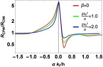
Figure 1: The resistance ratio $R_{CPW}/R_{CIW}$ vs the spin orbital coupling. In the plot, $\pi k_{f}/(mdh)=0.2$, $jh/v=1.06$. Different curves are for different cubic SOC terms. It is clear that the ratio approaches to the one when the SOC is much larger than the Zeeman energy $h$.

The minimum of the ratio is reached when

$$\alpha=\frac{\pi}{md}\ .$$ (40)

To understand this minimum, we consider the Hamiltonian with the linear SOC coupling only, ie. $\beta=0$. After the local $SU(2)$ gauge transformation, the Hamiltonian becomes

$$H= H_{0}+V+\mathrm{const.}$$ (41)

$$H_{0}= \frac{p^{2}}{2m}-h\sigma_{z}$$

$$V= \left(\alpha-\frac{\pi}{md}\right)\sigma_{x}p_{x}+\alpha\sigma_{y}\left(p_{y}\cos\theta+p_{z}\sin\theta\right)$$

$$+\alpha\sigma_{z}\left(p_{z}\cos\theta-p_{y}\sin\theta\right)$$ (42)

$$\mathrm{const}= \frac{\pi^{2}}{8md^{2}}-\frac{\alpha\pi}{2d}\ .$$

To simplify the notation, we define $\gamma=\alpha-\frac{\pi}{md}$. If SOC terms $\alpha k_{f}$, $\beta k_{f}^{3}$ are much smaller than the Zeeman energy, the eigenstate of the Hamiltonian can be solved based on perturbation. In addition, we assume that the impurity scattering is strongly spin-dependent, ie. $v\approx jh$. In this case, the conductivity is dominated by the outer Fermi surface, with its intraband impurity scattering given by

$$\left|M_{k\rightarrow k^{\prime}}^{++}\right|^{2}\approx(v+jh)^{2}\left[\frac{\gamma^{2}k_{x}k_{x}^{\prime}+\frac{\alpha^{2}}{2}(k_{y}k_{y}^{\prime}+k_{z}k_{z}^{\prime})}{4h^{2}}\right]^{2}$$ (43)

Here, $+$ is for outer Fermi surface. When $\alpha$ vanishes, it is clear that scattering is larger at larger $k_{x}$ and $k_{x}^{\prime}$. The resistivity comes from the fermions with larger momentum along the direction of the current. Therefore, $\rho_{x}\gg\rho_{y/z}$, and thus the ratio $R_{CPW}/R_{CIW}$ reaches its maximum. When $\gamma=0$ ($\alpha=\pi/(md)$), the scattering rate is larger for larger $k_{y/z}$ and $k^{\prime}_{y/z}$. Therefore, $\rho_{y/z}\gg\rho_{x}$, and the ratio $R_{CPW}/R_{CIW}$ reaches the minimum. More detailed information can be found in the appendix.

VI Anomalous Anisotropic Magnetoresistance

In previous sections, we have mainly focused on the effects of the linear SOC in Eq. (LABEL:fullHamiltonian). The cubic SOC only slightly modifies these effects. The cubic term fails to bring any qualitative change in these experiments. However from the symmetry’s point of view, only the cubic SOC breaks the $C_{4}$ rotation, and it must give rise to anisotropic behaviors of the magnetoresistance. To this end, we study the case when external magnetic field is sufficiently large to polarize all magnetic moments along its direction, and calculate the magnetoresistances. It is well known that for most of the cubic ferromagnets such as Ni, the anisotropic magnetoresistance (AMR) shows four fold symmetry when the magnetic field rotates in the plane perpendicular to the current. However it has already been reported that in B20 compounds such as Fe_1-xCo_xSiHuang et al. (2014a), the AMR shows anomalous behavior that only a two fold symmetry is respected. In this section, we will show how the cubic SOC leads to this observation.

The same model as the previous section is employed. The Hamiltonian and the impurity potential is in the same form as Eq. (37) and Eq. (38). The conductivity $\sigma_{zz}(\mathbf{h})$ is calculated while varying the magnetization $\mathbf{h}$ in the x-y plane. Most of the ferromagnetic materials have high symmetry and respect $C_{4}$ symmetry. Thus $\sigma_{zz}(h\hat{e}_{x})=\sigma_{zz}(h\hat{e}_{y})$ in these cases. However due to the $C_{4}$ breaking in B20 compounds, the anomalous AMR is expected where the ratio between two conductivities $\sigma_{zz}(h\hat{e}_{x})$ and $\sigma_{zz}(h\hat{e}_{y})$ deviates from $1$.

Before calculation, let’s explore the symmetries of the Hamiltonian in Eq. (37). It is found that

$$H(\alpha,\beta,h\hat{e}_{y})=SH(\alpha,-\beta,h\hat{e}_{x})S^{-1}$$ (44)

Here $S$ is the operator which rotates the system along $z$ axis by $\pi/2$. Therefore,

$$\sigma_{zz}(\alpha,\beta,h\hat{e}_{x})=\sigma_{zz}(\alpha,-\beta,h\hat{e}_{y})$$ (45)

In addition, the conductivity is invariant under the space inversion symmetry $P$,

$$H(-\alpha,-\beta,\boldsymbol{h})=PH(\alpha,\beta,\boldsymbol{h})P^{-1}$$ (46)

$$\Longrightarrow \sigma_{zz}(\alpha,\beta,\boldsymbol{h})=\sigma_{zz}(-\alpha,-\beta,\boldsymbol{h})$$

Combined with Eq. (45), it is concluded that

$$\sigma_{zz}(\alpha,\beta,h\hat{e}_{x})=\sigma_{zz}(\alpha,-\beta,h\hat{e}_{y})=\sigma_{zz}(-\alpha,\beta,h\hat{e}_{y})$$ (47)

Solely by symmetry argument, it is found that the anomalous AMR, defined as $\sigma_{zz}(h\hat{e}_{x})/\sigma_{zz}(h\hat{e}_{y})-1$, vanishes if either of two spin orbital couplings, $\alpha$ and $\beta$, vanishes. Similarly, we have $\sigma_{zz}(\alpha,\beta,h\hat{e}_{h})=\sigma_{zz}(\alpha,\beta,-h\hat{e}_{h})$.

In this section, the conductivity is calculated in the same way as the previous section. The Boltzmann equation is solved by perturbation method. The deviation of the electron distribution function is expanded by spherical harmonic functions up to $l=5$. The anisotropy comes from two different sources. (i) the Fermi surface is anisotropic since the Hamiltonian in Eq. (37) breaks $C_{4}$ symmetry. (ii) the eigenstate on the Fermi surface is anisotropic, and thus leads to the anisotropic impurity scattering by the spin-dependent potential in Eq. (38).

The energy of the Hamiltonian in Eq. (37) is given by

$$\varepsilon_{F} = \frac{\hbar^{2}k_{F}^{2}}{2m}\pm\Big{(}h_{z}^{2}+\alpha^{2}(k_{x}^{2}+k_{y}^{2}+k_{z}^{2})$$ (48)

$$+\beta^{2}[k_{x}^{2}(k_{y}^{2}-k_{z}^{2})^{2}+k_{y}^{2}(k_{z}^{2}-k_{x}^{2})^{2}+k_{z}^{2}(k_{x}^{2}-k_{y}^{2})^{2}]$$

$$+2h_{z}k_{z}[\alpha+\beta(k_{x}^{2}-k_{y}^{2})]\Big{)}^{1/2}$$

The system contains two Fermi surfaces (FSs) since the Kramers degeneracy is lifted. All terms in Eq. (48) respect the symmetry exchanging the indices $x$ and $y$ except the last term in square root. It shows explicitly that the Fermi surface asymmetry is possible only when then magnetization is nonzero.

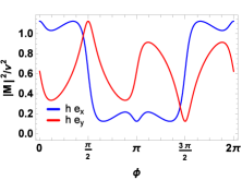
(a)

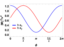
(b)

Figure 2: The intraband impurity scattering amplitude from $(0,0,k_{f})$ to $(k_{f}\cos\phi,k_{f}\sin\phi,0)$ on the outer Fermi surface. Red and blue curves are the scattering magnitude as a function of $\phi$ when the magnetization field points along $\hat{y}$ and $\hat{x}$ respectively, respectively. (a) The Zeeman energy is artificially turned off, while the impurity spin dependent is kept to be nonzero with $v/(jh)=2.0$ and $\beta k_{f}^{2}/\alpha=1.5$. The $C_{4}$ symmetry is broken in the impurity scattering amplitude. (b) $\beta=0$. Both the Zeeman energy and the impurity spin-dependent potential are nonzero with $h/(\alpha k_{f})=0.1$, and $v/(jh)=2.0$. It is clear that $C_{4}$ symmetry recovers for $\beta=0$.

However, the impurity scattering asymmetry is present as long as $\alpha$ and $\beta$ are non-zero. Fig. 2 shows the intraband scattering magnitude $|M|^{2}$ from $(0,0,k_{f})$ to $(k_{f}\cos\phi,k_{f}\sin\phi,0)$ on the outer Fermi surface. Red and blue curves are $|M|^{2}$ as a function of $\phi$ when the impurity magnetization points along $\hat{y}$ and $\hat{x}$, respectively. If the $C_{4}$ symmetry is kept, the blue curve should be the same as the red one after a translation of $\pi/2$, which is apparently not the truth. It is noticeable that even when Zeeman field vanishes, the impurity scattering still breaks the $C_{4}$ symmetry, although the shape of Fermi surface is still $C_{4}$ symmetric. Of course in reality, both the Zeeman term and spin-dependant scattering coexist.

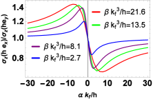
(a)

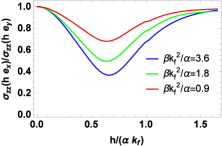
(b)

Figure 3: The ratio $\sigma_{z}(h\hat{e}_{x})/\sigma_{z}(h\hat{e}_{y})$ vs SOC couplings and the magnetization field. (a) The ratio as a function of SOC with $v/(jh)=2.0$. It becomes one when $\alpha=0$ or $\beta k_{f}^{2}/\alpha\rightarrow 0$. This agrees with our conclusion in Eq.(47) by symmetry argument. (b) The ratio vs Zeeman energy $h$ with $j=1.0$. The anomalous AMR vanishes when $h=0$ or $h\rightarrow\infty$.

Fig 3(a) shows the ratio $\sigma_{zz}(h\hat{e}_{x})/\sigma_{zz}(h\hat{e}_{y})$ as a function of the SOC. The ratio is smaller than $1$ when $\alpha$ and $\beta$ have the same sign, and larger than $1$ when two SOCs have different signs. This is consistent with the conclusion Eq. (47) derived by symmetry arguments. In addition, it is found that the anomalous AMR vanishes when either $\alpha=0$ or $\alpha\rightarrow\infty$. The latter implies that the anomalous AMR vanishes when $\beta\rightarrow 0$. This result agrees with our physical picture based on the Fermi surface topology. $C_{4}$ symmetry is restored on the Fermi surface when $\beta\rightarrow 0$.

Fig 3(b) shows the anomalous AMR as a function of the magnetization field $h$. When $h$ vanishes, not only the Zeeman energy vanishes, but also the impurity potential becomes spin-independent. Therefore, the impurity scattering becomes $C_{4}$ symmetric, as well as the Fermi surface. In this case, anomalous AMR vanishes. Our calculations agree well with the experimental resultsHuang et al. (2014a). When the temperature is raised above the Curie temperature, the anomalous AMR vanishes. This corresponds to the case with vanishing magnetization $\mathbf{h}$. In another limit when $h\rightarrow\infty$, the spin on the Fermi surface is fixed by the Zeeman energy. In this situation, the impurity scattering and Fermi surface become isotropic, and therefore the anomalous AMR vanishes.

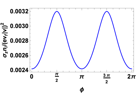
Figure 4: Conductivity vs direction of in-plane magnetization field. In the plot, $\alpha k_{f}/h=3.0$, $\beta k_{f}^{3}/h=5.4$, and $v/(jh)=2.0$. $n_{i}$ is the impurity density.

Fig 4 shows the variation of the conductivity $\sigma_{zz}$ as the direction of in-plane magnetization field changes. Note that $\sigma_{zz}$ reaches its minimum(maximum) when the field points along $x$($y$) direction. In our calculation, this comes from that assumption that two SOC couplings have the same sign. If $\alpha$ and $\beta$ have different signs, the minimum(maximum) is reached when $\boldsymbol{h}$ is along $y$($x$) axis. This result reproduces the experimental observations in Huang et al. (2014a).

VII conclusion

In conclusion, the spin-orbital coupling is the fountain of various interesting phenomena in B20 compounds. It not only provides the antisymmetric spin interactions, but also dramatically change behaviors of the electron transport. The effective Hamiltonian constructed in this work captures the main effects of the SOC in conduction electrons. Despite its simple form, the emergent new physics is closely associated with several experiments. It also calls for bunch of future works to study the spin transports related to this Hamiltonian. First principle calculations are also encouraged to determine the strength of the SOCs.

We are grateful for fruitful discussions with C. L. Chien, N. Nagaosa, S. X. Huang, C. X. Liu, O. Tchernyshyov, R. M. Fernandes, V. Galitski, and R. B. Tao. JK was supported by the Office of Basic Energy Sciences U.S. Department of Energy under awards numbers DE-SC0012336. JZ was supported by the TIPAC, by the U.S. Department of Energy under Award DEFG02-08ER46544, and by the National Science Foundation under Grant No. ECCS-1408168.

Supplementary for “Transport Theory of Metallic B20 Helimagnets”

I Solving Boltzmann Equation by Perturbation

If the Hamiltonian of the electron depends on the spin, the Kramer degeneracy will be lifted in the presence of a magnetic field. Even the single orbital Hamiltonian contains two different bands. The impurity potential induce not only intraband scattering, but also interband scattering. These scattering are, in general, highly anisotropic and therefore lead to many interesting phenomena. Although the relaxation time approximation, based on the assumption of isotropic system, may still be able to explain experiments qualitativelyDomainWall , it is questionable to produce a reliably quantitative description. We have to solve the Boltzmann equation without making any other assumptions. This section will describe a perturbative way to solve this equation. Note that the method presented here is not new, and has already been well explained in the textbookZiman .

I.1 Theory

We assume $f(k)=f_{0}(k)+f_{1}(k)$, where $f_{0}$ is the Fermi distribution function, or the distribution function at equilibrium. The Boltzmann equation can be written as

$$e\boldsymbol{E}\cdot\boldsymbol{v}_{+}(k)\left(\frac{\partial f_{0}}{\partial\epsilon}\right)_{\epsilon=\epsilon_{+}(k)} =2\pi n_{i}\int\frac{{\rm d}^{3}k^{\prime}}{(2\pi)^{3}}\Big{\{}\left(f_{1}^{+}(k^{\prime})-f_{1}^{+}(k)\right)T^{++}(k,k^{\prime})\delta\big{(}\epsilon_{+}(k)-\epsilon_{+}(k^{\prime})\big{)}+$$

$$\left(f_{1}^{-}(k^{\prime})-f_{1}^{+}(k)\right)T^{+-}(k,k^{\prime})\delta\big{(}\epsilon_{+}(k)-\epsilon_{-}(k^{\prime})\big{)}\Big{\}}$$ (S1)

$$e\boldsymbol{E}\cdot\boldsymbol{v}_{-}(k)\left(\frac{\partial f_{0}}{\partial\epsilon}\right)_{\epsilon=\epsilon_{-}(k)} =2\pi n_{i}\int\frac{{\rm d}^{3}k^{\prime}}{(2\pi)^{3}}\Big{\{}\left(f_{1}^{+}(k^{\prime})-f_{1}^{-}(k)\right)T^{-+}(k,k^{\prime})\delta\big{(}\epsilon_{-}(k)-\epsilon_{+}(k^{\prime})\big{)}+$$

$$\left(f_{1}^{-}(k^{\prime})-f_{1}^{-}(k)\right)T^{--}(k,k^{\prime})\delta\big{(}\epsilon_{-}(k)-\epsilon_{-}(k^{\prime})\big{)}\Big{\}}\ ,$$ (S2)

where the super(sub)scripts “$+/-$” refers to the two different bands due to removing Kramer degeneracy in the single electron Hamiltonian. $T^{\sigma,\sigma^{\prime}}(k,k^{\prime})$ is the scattering matrix element for electron from the state of $|\sigma,k\rangle$ to the state of $|\sigma^{\prime},k^{\prime}\rangle$. Thus, it contains both the intra-band and interband scattering. It is very easy to generalize to the Hamiltonian with more than two bands. Here, we will try the solution in the form of

$$f^{\pm}_{1}(k)=g_{\pm}(k)\left(-\frac{\partial f_{0}}{\partial\epsilon}\right)_{\epsilon=\epsilon_{\pm}(k)}\ .$$

The Boltzmann equation becomes

$$-e\boldsymbol{E}\cdot\boldsymbol{v}_{+}(k) =\frac{n_{i}}{(2\pi)^{2}}\int{\rm d}^{3}k^{\prime}\Big{\{}\left(g_{+}(k^{\prime})-g_{+}(k)\right)T^{++}(k,k^{\prime})\delta\big{(}\epsilon_{+}(k)-\epsilon_{+}(k^{\prime})\big{)}$$

$$\left(g_{-}(k^{\prime})-g_{+}(k)\right)T^{+-}(k,k^{\prime})\delta\big{(}\epsilon_{+}(k)-\epsilon_{-}(k^{\prime})\big{)}\Big{\}}$$ (S3)

$$-e\boldsymbol{E}\cdot\boldsymbol{v}_{-}(k) =\frac{n_{i}}{(2\pi)^{2}}\int{\rm d}^{3}k^{\prime}\Big{\{}\left(g_{+}(k^{\prime})-g_{-}(k)\right)T^{-+}(k,k^{\prime})\delta\big{(}\epsilon_{-}(k)-\epsilon_{+}(k^{\prime})\big{)}$$

$$\left(g_{-}(k^{\prime})-g_{-}(k)\right)T^{--}(k,k^{\prime})\delta\big{(}\epsilon_{-}(k)-\epsilon_{-}(k^{\prime})\big{)}\Big{\}}\$$ (S4)

$$\boldsymbol{j} =e\int\frac{{\rm d}^{3}k}{(2\pi)^{3}}\left(\boldsymbol{v}_{+}(k)g_{+}(k)\left(-\frac{\partial f_{0}}{\partial\epsilon}\right)_{\epsilon=\epsilon_{+}(k)}+\boldsymbol{v}_{-}(k)g_{-}(k)\left(-\frac{\partial f_{0}}{\partial\epsilon}\right)_{\epsilon=\epsilon_{-}(k)}\right)\ ,$$ (S5)

where $n_{i}$ is the density of impurity. To further simplify the notation, we can define the state vector and the linear operator

$$\Phi(k) =\begin{pmatrix}g_{+}(k)\\ g_{-}(k)\end{pmatrix}$$ (S6)

$$X(k) =-e\begin{pmatrix}\boldsymbol{E}\cdot\boldsymbol{v}_{+}(k)\\ \boldsymbol{E}\cdot\boldsymbol{v}_{-}(k)\end{pmatrix}$$ (S7)

$$(W\Phi)_{+}(k) =\frac{n_{i}}{(2\pi)^{2}}\int{\rm d}^{3}k^{\prime}\ \Big{\{}\left(g_{+}(k^{\prime})-g_{+}(k)\right)T^{++}(k,k^{\prime})\delta\big{(}\epsilon_{+}(k)-\epsilon_{+}(k^{\prime})\big{)}+$$

$$\hskip 28.45274pt\left(g_{-}(k^{\prime})-g_{+}(k)\right)T^{+-}(k,k^{\prime})\delta\big{(}\epsilon_{+}(k)-\epsilon_{-}(k^{\prime})\big{)}\Big{\}}$$ (S8)

$$(W\Phi)_{-}(k) =\frac{n_{i}}{(2\pi)^{2}}\int{\rm d}^{3}k^{\prime}\ \Big{\{}\left(g_{+}(k^{\prime})-g_{-}(k)\right)T^{-+}(k,k^{\prime})\delta\big{(}\epsilon_{-}(k)-\epsilon_{+}(k^{\prime})\big{)}+$$

$$\hskip 28.45274pt\left(g_{-}(k^{\prime})-g_{-}(k)\right)T^{--}(k,k^{\prime})\delta\big{(}\epsilon_{-}(k)-\epsilon_{-}(k^{\prime})\big{)}\Big{\}}$$ (S9)

It is clear that the Boltzmann equation can be written as

$$W\Phi(k)=X(k)\ .$$ (S10)

I.2 Approximation

We will work at $T=0$, so that the derivative of Fermi distribution function becomes a delta function. We will integrate our the magnitude of momentum and get the term $k^{2}/v_{k}$. Therefore, it is more convenient to define the “modified” scattering as

$$S^{\sigma\sigma^{\prime}}_{kk^{\prime}}=T^{\sigma\sigma^{\prime}}_{kk^{\prime}}\left(\frac{k^{2}}{v_{k}}\right)_{\sigma}\left(\frac{k^{2}}{v_{k}}\right)_{\sigma^{\prime}}\qquad Z_{\hat{n}}(k)=\begin{pmatrix}v^{+}_{n}\left(\frac{k^{2}}{v_{k}}\right)_{+}\\ v^{-}_{n}\left(\frac{k^{2}}{v_{k}}\right)_{-}\end{pmatrix}\ .$$

Clearly, in this definition, $S$ is symmetric, ie. $S^{\sigma\sigma^{\prime}}_{kk^{\prime}}=S^{\sigma^{\prime}\sigma}_{k^{\prime}k}$. In practice, we will expand the wave vector $\Phi(k)$ in terms of spherical harmonic functions. Define the matrix

$$M(k)=\begin{pmatrix}\left(\dfrac{k^{2}}{v_{k}}\right)_{+}&0\\ 0&\left(\dfrac{k^{2}}{v_{k}}\right)_{-}\end{pmatrix}\ ,$$

and multiply it on both sides of Boltzmann equation.

$$\sum_{\sigma^{\prime}l^{\prime}m^{\prime}}\left(S^{\sigma\sigma^{\prime}}(l,m;l^{\prime},m^{\prime})+(-)^{m+1}\delta_{\sigma\sigma^{\prime}}\sum_{l_{1}}\Big{(}\sum_{\sigma_{1}}S^{\sigma\sigma_{1}}(l_{1},m-m^{\prime};0,0)\Big{)}B(l_{1},m-m^{\prime};l^{\prime},m^{\prime};l)\right)g_{\sigma^{\prime}}(l^{\prime}m^{\prime})$$ (S11)

$$= Z_{\hat{n}}^{\sigma}(l,m)$$

$$g_{\sigma}(\hat{k}) =\sum_{lm}g_{\sigma}(l,m)Y_{l}^{m}(\hat{k})\ ,\qquad Z_{\hat{n}}^{\sigma}(\hat{k})=\sum_{lm}Z_{\hat{n}}^{\sigma}(l,m)Y_{l}^{m}(\hat{k})$$

$$S^{\sigma\sigma^{\prime}}(\hat{k},\hat{k}^{\prime}) =\sum_{lm}\sum_{l^{\prime}m^{\prime}}S^{\sigma\sigma^{\prime}}(l,m;l^{\prime},m^{\prime})\ Y_{l}^{m}(\hat{k})\left(Y_{l^{\prime}}^{m^{\prime}}(\hat{k}^{\prime})\right)^{*}$$

$$B(l_{1},m-m^{\prime};l^{\prime},m^{\prime};l) =(-)^{m}\sqrt{(2l_{1}+1)(2l^{\prime}+1)(2l+1)}\begin{pmatrix}l_{1}&l^{\prime}&l\\ m-m^{\prime}&m^{\prime}&-m\end{pmatrix}\begin{pmatrix}l_{1}&l^{\prime}&l\\ 0&0&0\end{pmatrix}$$

$$\sigma_{n} =\frac{1}{(2\pi)^{3}}\sum_{\sigma lm}(-)^{m}Z_{\hat{n}}^{\sigma}(l,m)g_{\sigma}(l,-m)$$

Note that the Wigner $3j$ symbol is used. Now, it is clear that we can solve the Boltzmann equations in an approximate way.

In practice, we will set a cutoff $l_{c}$ on the angular momentum of the spherical harmonic functions. Larger $l_{c}$ produces more precise solutions. In our calculation, we set $l_{c}=5$ for limitations on the computing source. We will see that it produces quantitatively different results from the relaxation time approximation.

II Helical Resistance

In this section, we will study the resistance of helical phase in the presence of the spin-orbital coupling. Apply the local $SU(2)$ gauge transformation in Eqn 39, the cubic SOC term becomes

$$R^{-1}\sigma_{x}k_{x}(k_{y}^{2}-k_{z}^{2})R= \sigma_{x}\left(k_{x}-\frac{2\pi}{d}\sigma_{x}\right)(k_{y}^{2}-k_{z}^{2})$$

$$R^{-1}\sigma_{y}k_{y}(k_{z}^{2}-k_{x}^{2})R\approx \big{(}\sigma_{y}\cos\theta-\sigma_{z}\sin\theta\big{)}k_{y}\left(k_{z}^{2}-\left(k_{x}-\frac{2\pi}{d}\sigma_{x}\right)^{2}\right)$$

$$R^{-1}\sigma_{y}k_{z}(k_{x}^{2}-k_{y}^{2})R\approx \big{(}\sigma_{z}\cos\theta+\sigma_{y}\sin\theta\big{)}k_{z}\left(\left(k_{x}-\frac{2\pi}{d}\sigma_{x}\right)^{2}-k_{y}^{2}\right)$$

With the assumption of $1/d\ll k_{f}$, it is safe to ignore the extra $2\pi/d$ terms in the transformed cubic SOC.

Fig 1 shows the ratio $R_{CPW}/R_{CIW}$ as a function of SOC. It is found that this ratio peaks when SOC vanishes and reaches its minimum when $\alpha=\pi h/(md)$ or $\gamma=0$. It is argued that the peaks and troughs are related with the anisotropy of the impurity scattering. In this section, we investigate the scattering more systematically, and reveals how the anisotropy of the scattering is changed by SOC.

As in the main text, we consider the case $\beta=0$ for simplicity. The Hamiltonian is

$$H= H_{0}+V$$

$$H_{0}= \frac{p^{2}}{2m}-h\sigma_{z}$$

$$V= \gamma\sigma_{x}p_{x}+\alpha\sigma_{y}\left(p_{y}\cos\theta+p_{z}\sin\theta\right)+\alpha\sigma_{z}\left(p_{z}\cos\theta-p_{y}\sin\theta\right)$$

$$U= v\ \mathrm{I}_{2\times 2}-jh\sigma_{z}$$

Here $\gamma=\alpha-\pi/(md)$ and $U$ is the transformed impurity potential. For small SOC $\alpha k_{f}\ll h$, we treat $V$ as the perturbation and calculate the wavefunction.

$$|+,k\rangle =N_{+}^{-1}(k_{+})\left[\begin{pmatrix}e^{ik_{+}r}\\ 0\end{pmatrix}-\dfrac{\gamma k_{x}+i\alpha\left(k_{y}\cos\theta+k_{z}\sin\theta\right)}{2h}\begin{pmatrix}0\\ e^{ik_{+}r}\end{pmatrix}\right]$$

$$|-,k\rangle =N_{-}^{-1}(k_{+})\left[\begin{pmatrix}0\\ e^{ik_{-}r}\end{pmatrix}+\dfrac{\gamma k_{x}-i\alpha\left(k_{y}\cos\theta+k_{z}\sin\theta\right)}{2h}\begin{pmatrix}e^{ik_{+}r}\\ 0\end{pmatrix}\right]$$

$N_{\pm}$ are introduced for normalization. In principle, $\theta=2\pi x/d$ is a space dependent function, and thus will mix the plane wave with different momentum and different fermi surfaces. Here, it is assumed that the space varying is much smaller than the difference of two fermi momentum. Especially, $1/d\ll||k_{-}-k_{+}|$, ie. it will not mix two Fermi surfaces. Now, we calculate the scattering matrix elements in the case of strongly spin-dependent impurity potential, eg. $v\approx jh$. After integrating over $\theta(x)$.

$$T^{++}(k,k^{\prime}) =\left|\langle+k^{\prime}|U|+k\rangle\right|^{2}\approx\left(\frac{v+jh}{(2h)^{2}}\right)^{2}\left(\gamma^{2}k_{x}k_{x}^{\prime}+\frac{\alpha^{2}}{2}\left[k_{y}k_{y}^{\prime}+k_{z}k_{z}^{\prime}\right]\right)^{2}$$ (S12)

$$T^{--}(k,k^{\prime}) =\left|\langle-k^{\prime}|U|-k\rangle\right|^{2}\approx(v+jh)^{2}$$

$$T^{+-}(k,k^{\prime}) =\left|\langle-k^{\prime}|U|+k\rangle\right|^{2}\approx\frac{\gamma^{2}}{(2h)^{2}}\left[(v+jh)k_{x}-(v-jh)k_{x}^{\prime}\right]^{2}+\frac{1}{2}\frac{\alpha^{2}}{(2h)^{2}}\left[\left((v+jh)k_{y}+(v-jh)k_{y}^{\prime}\right)^{2}+(k_{y}\leftrightarrow k_{z})\right]$$

It is easy to see that $T^{++}\ll T^{--}$. The conductivity is dominated by the fermi surface with smaller intraband scattering as those parts with large scattering rate will be “shorted out” BZShort . Therefore, we focus only on $T^{++}$ here.

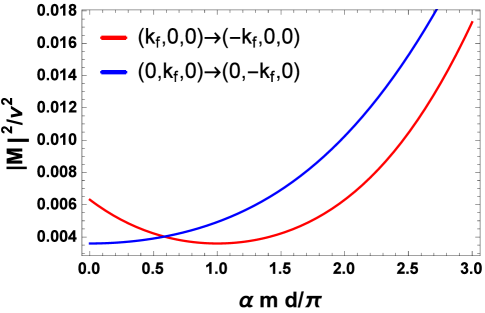
Figure S1: Scattering magnitude vs. the spin orbital coupling $\alpha$ with $jh/v=1.06$, and $\beta=0$. Red: Scattering between $(k_{f},0,0)$ and $(-k_{f},0,0)$. It is clear that the scattering rate reaches its minimum when $\alpha\approx\pi/(md)$. This behavior is typical for the scattering between large $k_{x}$, which accounts for the resistivity when current is perpendicular to the domain wall. Blue: Scattering between $(0,k_{f},0)$ and $(0,-k_{f},0)$. It monotonically increase with SOC. This is common among the scattering between large $k_{y}$ ($k_{z}$) which accounts for the resistivity when current is parallel to the domain wall.

For currents perpendicular to the domain wall (along $\hat{x}$), the electrons contributed to this flow are dominated by those with larger $k_{x}$ since the velocity $v_{x}\approx k_{x}/m$. For currents parallel to the domain wall, the electrons contributed to this flow are dominated by those with larger $k_{y}$($k_{z}$) since the velocity $v_{x}\approx k_{x}/m$ ($v_{y}\approx k_{y}/m$). When SOC vanishes $\alpha=0$, $\gamma\neq 0$, larger $k_{x}$ and $k_{x}^{\prime}$ leads to larger scattering in Eqn S12. Therefore, $R_{CPW}\gg R_{CIW}$, and the ratio reaches its maximum. When $\alpha=\pi/(md)$, $\gamma=0$, $\alpha\neq 0$, larger $k_{y}$ and $k_{y}^{\prime}$ (or $k_{z}$ and $k_{z}^{\prime}$) leads to larger scattering. Therefore, $R_{CIW}\gg R_{CPW}$, and the minimum of ratio emerges. When SOC becomes very large, spin on the fermi surface is locked by the direction of the fermi momentum. In this limit, the anisotropy of the scattering vanishes and the ratio approaches to $1$, as shown in Fig S1.

References

- Schlesinger et al. (1993) Z. Schlesinger, Z. Fisk, H.-T. Zhang, M. B. Maple, J. DiTusa, and G. Aeppli, Physical Review Letters 71, 1748 (1993), URL http://link.aps.org/doi/10.1103/PhysRevLett.71.1748.
- DiTusa et al. (1997) J. F. DiTusa, K. Friemelt, E. Bucher, G. Aeppli, and A. P. Ramirez, Physical Review Letters 78, 2831 (1997), URL http://link.aps.org/doi/10.1103/PhysRevLett.78.2831.
- Mühlbauer et al. (2009) S. Mühlbauer, B. Binz, F. Jonietz, C. Pfleiderer, A. Rosch, A. Neubauer, R. Georgii, and P. Böni, Science 323, 915 (2009), ISSN 0036-8075, 1095-9203, URL http://www.sciencemag.org/content/323/5916/915.
- Pfleiderer et al. (2004) C. Pfleiderer, D. Reznik, L. Pintschovius, H. v. Löhneysen, M. Garst, and A. Rosch, Nature 427, 227 (2004), ISSN 0028-0836, URL http://www.nature.com/nature/journal/v427/n6971/abs/nature022%%****␣B20T.tex␣Line␣1075␣****32.html.
- Ritz et al. (2013) R. Ritz, M. Halder, M. Wagner, C. Franz, A. Bauer, and C. Pfleiderer, Nature 497, 231 (2013), ISSN 0028-0836, URL http://www.nature.com/nature/journal/v497/n7448/abs/nature120%23.html.
- Huang and Chien (2012) S. X. Huang and C. L. Chien, Phys. Rev. Lett. 108, 267201 (2012), URL http://link.aps.org/doi/10.1103/PhysRevLett.108.267201.
- Yu et al. (2011) X. Z. Yu, N. K. anazawa, Y. Onose, K. Kimoto, W. Z. Zhang, S. Ishiwata, Y. Matsui, and Y. Tokura, Nat Mater 10, 106 (2011), URL http://www.nature.com/nmat/journal/v10/n2/abs/nmat2916.html.
- Seki et al. (2012) S. Seki, X. Z. Yu, S. Ishiwata, and Y. Tokura, Science 336, 198 (2012), URL http://www.sciencemag.org/content/336/6078/198.full.html.
- Uchida et al. (2006) M. Uchida, Y. Onose, Y. Matsui, and Y. Tokura, Science 311, 359 (2006), ISSN 0036-8075, 1095-9203, URL http://www.sciencemag.org/content/311/5759/359.
- Dzyaloshinsky (1958) I. Dzyaloshinsky, Journal of Physics and Chemistry of Solids 4, 241 (1958), ISSN 0022-3697, URL http://www.sciencedirect.com/science/article/pii/002236975890%0763.
- Moriya (1960) T. Moriya, Physical Review 120, 91 (1960), URL http://link.aps.org/doi/10.1103/PhysRev.120.91.
- Skyrme (1961) T. H. R. Skyrme, Proceedings of the Royal Society of London. Series A. Mathematical and Physical Sciences 260, 127 (1961), ISSN 1364-5021, 1471-2946, URL http://rspa.royalsocietypublishing.org/content/260/1300/127.
- Yu et al. (2010) X. Z. Yu, Y. Onose, N. Kanazawa, J. H. Park, J. H. Han, Y. Matsui, N. Nagaosa, and Y. Tokura, Nature 465, 901 (2010), ISSN 0028-0836, URL http://www.nature.com/nature/journal/v465/n7300/full/nature09%124.html.
- Rö\ssler et al. (2006) U. K. Rö\ssler, A. N. Bogdanov, and C. Pfleiderer, Nature 442, 797 (2006), ISSN 0028-0836, URL http://www.nature.com/nature/journal/v442/n7104/full/nature05%056.html.
- Kadowaki et al. (1982) K. Kadowaki, K. Okuda, and M. Date, Journal of the Physical Society of Japan 51, 2433 (1982), ISSN 0031-9015, URL http://journals.jps.jp/doi/abs/10.1143/JPSJ.51.2433.
- Du et al. (2014) H. Du, J. P. DeGrave, F. Xue, D. Liang, W. Ning, J. Yang, M. Tian, Y. Zhang, and S. Jin, Nano Letters 14, 2026 (2014), ISSN 1530-6984, URL http://dx.doi.org/10.1021/nl5001899.
- Zang et al. (2011) J. Zang, M. Mostovoy, J. H. Han, and N. Nagaosa, Physical Review Letters 107, 136804 (2011), URL http://link.aps.org/doi/10.1103/PhysRevLett.107.136804.
- Schulz et al. (2012) T. Schulz, R. Ritz, A. Bauer, M. Halder, M. Wagner, C. Franz, C. Pfleiderer, K. Everschor, M. Garst, and A. Rosch, Nature Physics 8, 301 (2012), ISSN 1745-2473, URL http://www.nature.com/nphys/journal/v8/n4/full/nphys2231.html%.
- Neubauer et al. (2009) A. Neubauer, C. Pfleiderer, B. Binz, A. Rosch, R. Ritz, P. G. Niklowitz, and P. Böni, Physical Review Letters 102, 186602 (2009), URL http://link.aps.org/doi/10.1103/PhysRevLett.102.186602.
- Lee et al. (2009) M. Lee, W. Kang, Y. Onose, Y. Tokura, and N. P. Ong, Physical Review Letters 102, 186601 (2009), URL http://link.aps.org/doi/10.1103/PhysRevLett.102.186601.
- Kanazawa et al. (2011) N. Kanazawa, Y. Onose, T. Arima, D. Okuyama, K. Ohoyama, S. Wakimoto, K. Kakurai, S. Ishiwata, and Y. Tokura, Phys. Rev. Lett. 106, 156603 (2011), URL http://link.aps.org/doi/10.1103/PhysRevLett.106.156603.
- Li et al. (2013) Y. Li, N. Kanazawa, X. Z. Yu, A. Tsukazaki, M. Kawasaki, M. Ichikawa, X. F. Jin, F. Kagawa, and Y. Tokura, Physical Review Letters 110, 117202 (2013), URL http://link.aps.org/doi/10.1103/PhysRevLett.110.117202.
- Watanabe et al. (2014) H. Watanabe, S. A. Parameswaran, S. Raghu, and A. Vishwanath, Physical Review B 90, 045145 (2014), URL http://link.aps.org/doi/10.1103/PhysRevB.90.045145.
- Huang et al. (2014a) S. X. Huang, F. Chen, J. Kang, J. Zang, G. J. Shu, F. C. Chou, and C. L. Chien, arXiv:1409.7867 [cond-mat] (2014a), arXiv: 1409.7867, URL http://arxiv.org/abs/1409.7867.
- Huang et al. (2014b) S. X. Huang, J. Kang, F. Chen, J. Zang, G. J. Shu, F. C. Chou, S. V. Grigoriev, V. A. Dyadkin, and C. L. Chien, arXiv:1409.7869 [cond-mat] (2014b), arXiv: 1409.7869, URL http://arxiv.org/abs/1409.7869.
- Winkler (2003) R. Winkler, Spin–Orbit Coupling Effects in Two-Dimensional Electron and Hole Systems, Springer Tracts in Modern Physics (Springer, 2003).
- Dresselhaus et al. (2010) M. S. Dresselhaus, G. Dresselhaus, and A. Jorio, Group Theory: Application to the Physics of Condensed Matter (Springer, Berlin, 2010), softcover reprint of hardcover 1st ed. 2008 edition ed., ISBN 9783642069451.
- Jeong and Pickett (2004) T. Jeong and W. Pickett, Physical Review B 70, 075114 (2004), URL http://link.aps.org/doi/10.1103/PhysRevB.70.075114.
- Koster (1957) G. F. Koster, Space Groups and Their Representations (Academic Press, 1957), ISBN 9780124337848.
- Žutić et al. (2004) I. Žutić, J. Fabian, and S. Das Sarma, Reviews of Modern Physics 76, 323 (2004), URL http://link.aps.org/doi/10.1103/RevModPhys.76.323.
- Leonov (2014) A. O. Leonov, arXiv:1406.2177 [cond-mat] (2014), arXiv: 1406.2177, URL http://arxiv.org/abs/1406.2177.
- Ruderman and Kittel (1954) M. A. Ruderman and C. Kittel, Physical Review 96, 99 (1954), URL http://link.aps.org/doi/10.1103/PhysRev.96.99.
- Kasuya (1956) T. Kasuya, Progress of Theoretical Physics 16, 45 (1956), ISSN 0033-068X, 1347-4081, URL http://ptp.oxfordjournals.org/content/16/1/45.
- Yosida (1957) K. Yosida, Physical Review 106, 893 (1957), URL http://link.aps.org/doi/10.1103/PhysRev.106.893.
- Fert et al. (2013) A. Fert, V. Cros, and J. Sampaio, Nature nanotechnology 8, 152 (2013), URL http://dx.doi.org/10.1038/nnano.2013.29.
- Bazaliy et al. (1998) Y. B. Bazaliy, B. A. Jones, and S.-C. Zhang, Physical Review B 57, R3213 (1998), URL http://link.aps.org/doi/10.1103/PhysRevB.57.R3213.
- Tatara and Kohno (2004) G. Tatara and H. Kohno, Physical Review Letters 92, 086601 (2004), URL http://link.aps.org/doi/10.1103/PhysRevLett.92.086601.
- Bauer and Pfleiderer (2012) A. Bauer and C. Pfleiderer, Physical Review B 85, 214418 (2012), URL http://link.aps.org/doi/10.1103/PhysRevB.85.214418.
- Levy and Zhang (1997) P. M. Levy and S. Zhang, Physical Review Letters 79, 5110 (1997), URL http://link.aps.org/doi/10.1103/PhysRevLett.79.5110.

References

- (1) P. M. Levy, and S. Zhang, Phys. Rev. Lett. 79, 5110 (1997).
- (2) R. Hlubina and T. M. Rice, Phys. Rev. B. 51, 9253 (1995).
- (3) Ziman, Electrons and Phonons (Clarendon, Oxford, 1960).