GRAPHITE: An Extensible Graph Traversal Framework
for Relational Database Management Systems

Abstract

Graph traversals are a basic but fundamental ingredient for a variety of graph algorithms and graph-oriented queries. To achieve the best possible query performance, they need to be implemented at the core of a database management system that aims at storing, manipulating, and querying graph data. Increasingly, modern business applications demand native graph query and processing capabilities for enterprise-critical operations on data stored in relational database management systems. In this paper we propose an extensible graph traversal framework (graphite) as a central graph processing component on a common storage engine inside a relational database management system.

We study the influence of the graph topology on the execution time of graph traversals and derive two traversal algorithm implementations specialized for different graph topologies and traversal queries. We conduct extensive experiments on graphite for a large variety of real-world graph data sets and input configurations. Our experiments show that the proposed traversal algorithms differ by up to two orders of magnitude for different input configurations and therefore demonstrate the need for a versatile framework to efficiently process graph traversals on a wide range of different graph topologies and types of queries. Finally, we highlight that the query performance of our traversal implementations is competitive with those of two native graph database management systems.

1 Introduction

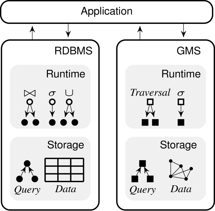
(a) Separated rdbms and gms with specialized storage engines and processing via application.

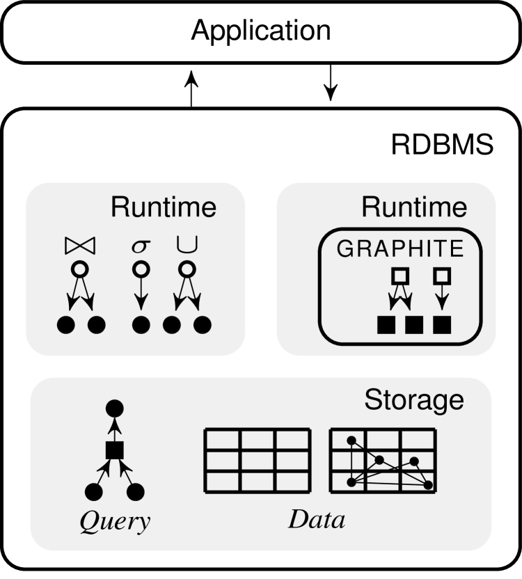
(b) rdbms with integrated graph processing capabilities and common storage engine.

Figure 1: Architecture alternatives for graph processing.

Evermore, enterprises from various domains, such as the financial, insurance, and pharmaceutical industry, explore and analyze the connections between data records in traditional customer-relationship management and enterprise-resource-planning systems. Typically, these industries rely on mature rdbms technology to retain a single source of truth and access. Although graph structure is already latent in the relational schema and inherently represented in foreign key relationships, managing native graph data is moving into focus as it allows rapid application development in the absence of an upfront defined database schema. Specifically, novel and traditional business applications leverage the advantages of a graph data model, such as schema flexibility and an explicit representation of relationships between data records. Although these business applications mainly operate on graph-structured data, they still require direct access to the relational base data.
Existing solutions performing graph operations on business-critical data either use a combination of sql and application logic or employ a graph management system (gms) such as Neo4j [3] or Sparksee [24], or distributed graph systems, such as GraphLab [21] or Apache Giraph [1]. For the first approach, relying only on sql typically results in poor execution performance caused by the functional mismatch between a traversal algebra [29] and the relational algebra. Even worse, the relational query optimizer is not graph-aware i.e., it does not keep statistics about the graph topology nor about graph query patterns, and therefore is likely to construct a suboptimal execution plan. The other alternative is to process the data in a native gms to hurdle the unsuitability of the relational algebra to express complex graph queries in an rdbms.

Figure 1(a) depicts a traditional system landscape with an rdbms and a gms located next to each other and orchestrated at application level. A gms is superior to an rdbms for complex graph processing as it provides a natural understanding of a graph data model, a rich set of graph processing functionality, and optimized data structures for fast data access. Especially scenarios that do not require accessing the most recent data snapshot nor combine operations from different data models into cross-data-model operations can be handled by gms’s efficiently. Cross-data-model operations combining data from various data models, i.e., relational, text, spatial, temporal, and graph however will play a key role for graph analytics in the future [5]. For example, a clinical information system stores data from patient records in an rdbms. Graph analytics on a knowledge graph of patient records and their relationships to each other help physicians to improve diagnostics and identify complex co-morbidity conditions. Such a medical knowledge graph contains not only information about the relationships between diagnoses and patients, but also text data from patient records and temporal information about prescriptions.

In this paper we propose the seamless integration of graph processing functionality into an rdbms sharing a common storage engine as depicted in Figure 1(b). Located next to a relational runtime stack in the same system, a graph runtime with a set of graph operators provides native support for querying graph data on top of a common relational storage engine. For the context of this paper, we focus on graph traversals as they are a vital component of every gms and the foundation for a large variety of graph algorithms, such as finding shortest paths, detecting connected components, and answering reachability queries.
We introduce graphite, a traversal framework that provides an extensible set of logical graph traversal operators and their corresponding implementations. Similar to the distinction between a logical and a physical layer in a relational runtime, graphite also provides a set of logical operators and a set of corresponding physical implementations. In the context of this paper we propose two traversal implementations optimized for in-memory columnar rdbms but argue that the general concept of a traversal framework can be extended with specialized traversal implementations and cost models for row-oriented or even disk-based rdbms. graphite operates on a physical column group model (cf. Figure 2). We summarize our main contributions as follows:

• We introduce graphite as a modular and extensible foundation of a traversal framework inside an rdbms, which allows seamlessly reusing existing physical data structures and deploying of novel traversal implementations.

• We present two different implementations of the traversal operator, a naive level-synchronous (ls), and a novel fragmented-incremental (fi) traversal algorithm that is superior to the naive approach for specific graph topologies and traversal queries.

• We conduct an extensive experimental evaluation for a large variety of real-world data sets and traversal queries, and show an execution time improvement of our fi-traversal by up to two orders of magnitude compared to the ls-traversal for certain graph topologies and traversal queries. Moreover, we show that the query performance of our implementations is competitive with those of two native graph database management systems.

The remainder of this paper is structured as follows: in Section 2, we describe graphite as the foundation of the traversal operator that we present in Section 3. We detail the two physical implementations of the traversal operator in Sections 4 and 5, respectively. A set of topology-aware clustering techniques that can be applied to both physical implementations is presented in Section 6. In Section 7 we provide an extensive experimental evaluation of our traversal implementations. Finally, we discuss related work in Section 8 before we conclude the paper in Section 9.

2 Graph Traversal Framework

graphite is a general and extensible framework that allows easy deploying, testing, and benchmarking of traversal implementations on top of a common relational storage engine of an rdbms. It provides a common interface for traversal configuration parameters and is tightly integrated with a unified, graph-aware controller infrastructure leveraging a comprehensive set of available graph statistics. We show that the query optimizer of an rdbms can benefit from having extensive information about the graph topology to choose the best traversal operator for a given traversal query.

Graph Model and Physical Representation

graphite provides as logical data model a property graph model. The property graph data model has emerged as the de-facto standard for general purpose graph processing in enterprise environments [28]. It represents multi-relational directed graphs where vertices and edges can have assigned an arbitrary number of attributes in a key/value fashion.
We store a property graph using a common storage infrastructure with the relational runtime stack in two column groups, one for the vertices and one for the edges, respectively. A column group represents a column-oriented data layout, where a new attribute can be added by appending a new column to the column group [7]. Null values in sparsely populated columns can be compressed through run-length-based compression techniques [6]. Additionally, the evaluation of column predicates allows a seamless combination of relational predicate filters with the actual traversal operation. Figure 2 depicts an example graph and its mapping to two column groups. We map each vertex and edge to a single entry in the column group and each attribute to a separate column. Each vertex has a unique identifier as the only mandatory attribute.

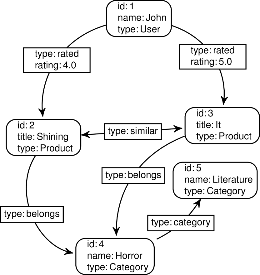
(a) Example graph.

$id$	$type$	$name$	$title$	$\ldots$
1	User	John	?	$\ldots$
2	Product	?	Shining
3	Product	?	It	$\ldots$
4	Category	Horror	?
5	Category	Literature	?	$\ldots$

(b) Vertex column group.

$V_{s}$	$V_{t}$	$type$	$rating$	$\ldots$
2	3	similar	?	$\ldots$
2	4	belongs	?
3	4	belongs	?	$\ldots$
1	3	rated	5.0
1	2	rated	4.0	$\ldots$
4	5	category	?

(c) Edge column group.

Figure 2: Mapping of a property graph to column groups.

Traversal Configuration

In the following, we introduce a formal notion of the graph traversal operation, its input parameters, and the expected output.

Definition 1

(Traversal Configuration) Let $G=(V,E)$ be a directed, multi-relational graph, where $V$ refers to the set of vertices and $E\subseteq(V\times V)$ refers to the set of edges. We define a traversal configuration $\rho$ as a tuple $\rho=(S,\varphi,c,r,d)$ composed of a set of start vertices $S\subseteq V$, an edge predicate $\varphi$, a collection boundary $c$, a recursion boundary $r$, and a traversal direction $d$. A graph traversal $\tau_{G}(\rho)$ is a unary operation on $G$ and returns a set of visited vertices $R\subseteq V$.

We represent each vertex in $S$ by its unique vertex identifier. The edge predicate $\varphi$ defines a propositional formula consisting of atomic attribute predicates that can be combined with the logical operators $\land$, $\lor$, and $\neg$. For each edge $e\in E$, the traversal algorithm evaluates $\varphi$ and appends matching edges to the working set of active edges. Further, it receives a recursion boundary $r\in\mathbb{N}^{+}$ that defines the maximum number of levels to traverse. To support unlimited traversals or transitive closure calculations, the recursion boundary can be infinite ($\infty$). The collection boundary $c\in\mathbb{N}$ specifies the level of the traversal from where to start collecting discovered vertices. For $c=0$, we add all start vertices to the result. For any traversal configuration, the condition $c\leq r$ must hold. The traversal direction $d\in\Set{\rightarrow,\leftarrow}$ specifies the direction to traverse the edges. A forward traversal ($\rightarrow$) traverses edges from the source vertex to the target vertex, a backward traversal ($\leftarrow$) traverses edges in the opposite direction. The traversal operation outputs a set of vertices that have been visited in the boundaries defined by $c$ and $r$.

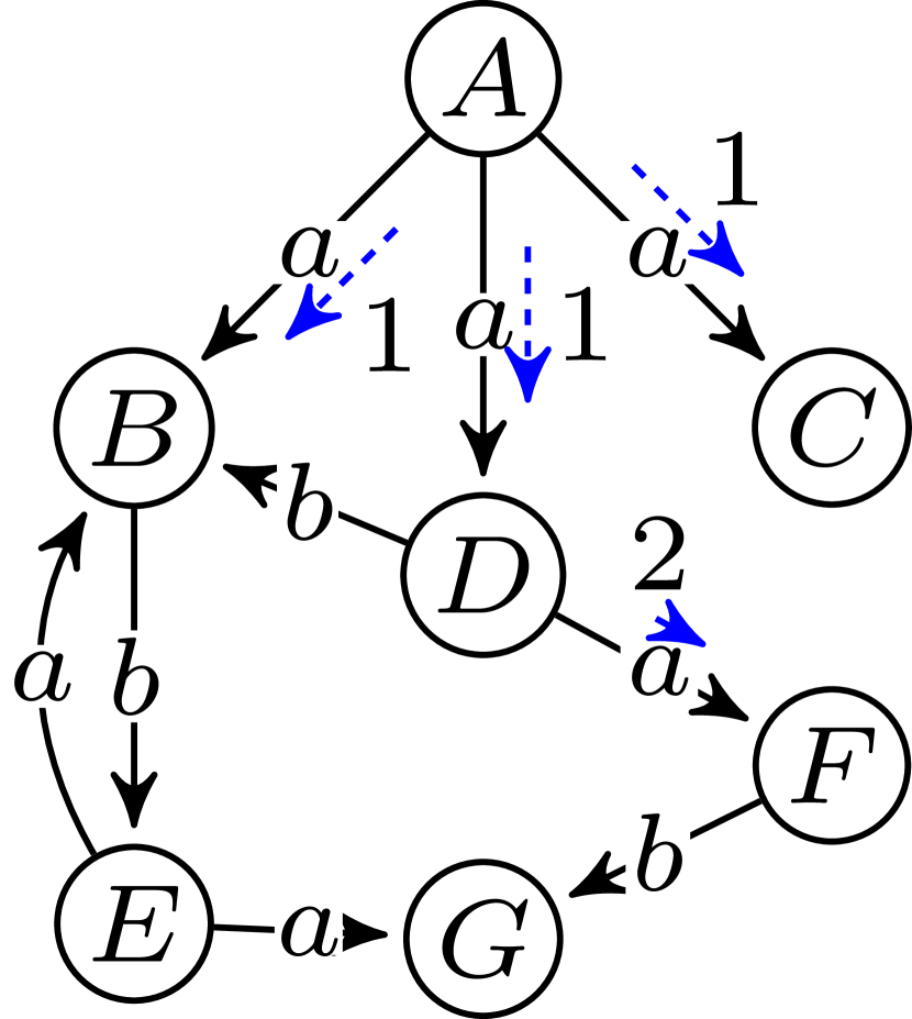
Traversal Configuration	Result
$(\Set{A},\text{'\emph{type=a}'},0,1,\rightarrow)$	$\Set{A,B,C,D}$
$(\Set{A},\text{'\emph{type=a}'},0,1,\rightarrow)$	$\Set{A,B,C,D}$
$(\Set{A},\text{'\emph{type=a}'},1,1,\rightarrow)$	$\Set{B,C,D}$
$(\Set{A},\text{'\emph{type=a}'},2,2,\rightarrow)$	$\Set{F}$
$(\Set{A},\text{'\emph{type=a}'},1,\infty,\rightarrow)$	$\Set{B,C,D,F}$
$(\Set{E},\text{'\emph{type=b}'},2,2,\leftarrow)$	$\Set{D}$
$(\Set{A},\text{'\emph{type=a $\vee$ type=b}'},2,2,\rightarrow)$	$\Set{E,F}$

Figure 3: Traversal configurations and result sets.

Formal Description

We define a traversal by a totally ordered set $P$ of path steps, where each path step describes the transition between two traversal iterations. Path steps are evaluated sequentially according to the total ordering in $P$. We determine the number of path steps by the recursion boundary $r$. Formally, we define a graph traversal operation based on the mathematical notion of sets and their basic operations union and complement. Each path step $p_{i}\in P$ with $1\leq i\leq r$ receives a set of vertices $D_{i-1}$ discovered at level $i-1$ and returns a set of adjacent vertices $D_{i}$. Initially, we assign the set of start vertices to the set of discovered vertices ($D_{0}=S$). In the following, we define the transformation rules for $p_{i}$ with $i>0$.

$$D_{i}^{\rightarrow}=\Set{v}{\exists u\in D_{i-1}:e=(u,v)\in E\wedge eval(e,\varphi)}$$ (1)

$$D_{i}^{\leftarrow}=\Set{u}{\exists v\in D_{i-1}:e=(u,v)\in E\wedge eval(e,\varphi)}$$ (2)

Depending on the traversal direction $d$, we select a different transformation rule. Equation 1 presents the definition for forward traversals ($\rightarrow$), and Equation 2 for backward traversals ($\leftarrow$), respectively. In path step $p_{i}$ we generate the set of vertices $D_{i}$ by traversing from each vertex in $D_{i-1}$ over all outgoing/incoming edges matching the edge predicate $\varphi$. Once the traversal operation finished processing the path step, the vertex set $D_{i}$ contains all vertices reachable within one hop from the vertices in $D_{i-1}$ via edges for which $\varphi$ holds. Equation 3 shows the definition of the resulting vertex set $R_{\tau}$ for a traversal operation $\tau$.

$$R_{\tau}=\Bigg{(}\underbrace{\bigcup\limits_{i=c}^{r}D_{i}}_{\text{target vertices}}\Bigg{)}\setminus\Bigg{(}\underbrace{\bigcup\limits_{i=0}^{c-1}D_{i}}_{\text{visited vertices}}\Bigg{)}$$ (3)

Conceptually, the collection boundary $c$ and the recursion boundary $r$ divide the discovered vertices into two working sets. The set of visited vertices contains all vertices that have been discovered before the traversal reached the collection boundary $c$. Vertices within the set of visited vertices are not considered for the final result, but are necessary to complete the traversal operation. We produce the set of visited vertices by forming the union of all partial vertex sets $\{D_{0},D_{1},\ldots,D_{c-1}\}$ from path steps $p_{1}$ to $p_{c-1}$. The set of target vertices refers to the set of vertices that are potentially relevant for the final result set. To produce the set of target vertices, we union all partial vertex sets $\{D_{c},\ldots,D_{r}\}$ from path steps $p_{c}$ to $p_{r}$. To retrieve the final result, we compute the complement between the set of target vertices and the set of visited vertices. We consider only vertices from the set of target vertices that are not in the set of visited vertices for the final result. Figure 3 shows a set of example traversal configurations and their query results for the given graph.

Example. Traversal configuration $(\Set{A},\text{'\emph{type=a}'},2,2,\rightarrow)$ in Figure 3 traverses starting from vertex $A$ on edges of type $a$ and visits all vertices within a distance of 2 from vertex $A$. Here, we only collect discovered vertices in the last path step $p_{2}$. Dashed arrows with numbers show the traversed edges and the path step they were discovered in. First, path step $p_{1}$ transforms the vertex set $D_{0}=\Set{A}$ into the vertex set $D_{1}=\Set{B,C,D}$. Next, path step $p_{2}$ transforms vertex set $D_{1}$ into vertex set $D_{2}=\Set{F}$. Finally, the output for this example graph and traversal configuration is a vertex set containing vertex $F$ only.

3 Traversal Operators

We now discuss the components of graphite, as shown in Figure 4, in detail. It receives a traversal configuration $\rho$ and processes a traversal in three phases: a Preparation Phase, a Traversal Phase, and a Decoding Phase. All three phases share common interfaces allowing to easily exchange implementations.

Figure 4: Processing phases in graphite.

Preparation Phase

We pass a set of start vertices $S$ to the preparation phase and transform it into a more processing-friendly set-oriented data structure. If the storage engine leverages dictionary encoding [6], we consult the value dictionary of the source/target vertex column in the edge column group, and encode all vertices from $S$ into their internal numerical value code representation. Depending on the traversal direction, we use a different vertex ID column (either $V_{s}$ or $V_{t}$ from Figure 2). In addition to the actual value encoding, we select active edges that are to be considered for the traversal operation. Therefore, we push down the edge predicate $\varphi$ to the storage engine to filter out invalid edges. Active edges are stored in a list that represents the valid and invalid records of a column group. Additionally, transactional visibility is guaranteed by intersecting the obtained list with visibility information in the current transaction context from the multi-version concurrency control of the rdbms. Finally, we pass the list of active edges to the traversal phase for further processing.

Traversal Phase

We distinguish two major components in the traversal phase: a set of traversal operator implementations and a traversal controller. Within the scope of this paper, we propose two traversal algorithm strategies—level-synchronous and fragmented-incremental—and describe them in detail in Sections 4 and 5, respectively. Initially, we pass a collection boundary $c$, a recursion boundary $r$, a traversal direction $d$, a set of active edges $E_{\textit{a}}$, and the encoded vertex set $S$ to the traversal phase. We select the best traversal operator implementation based on collected graph statistics and the characteristics of the traversal query. After the traversal operator has finished execution, it returns discovered vertices in a set-oriented data structure.

Decoding Phase

To translate the internal code representations of discovered vertices back into actual ID values, we consult the value dictionary of the source/target vertex column for each value code and add the actual value to the final output set. If the storage engine does not leverage dictionary encoding, the decoding phase can be omitted and the result set directly returned.

3.1 Strategies and Variations

The core component of an implementation of the graph traversal operator is the traversal algorithm. In general, traversal algorithms occur in variations favoring different graph topologies and traversal queries. While dense graphs with a large vertex outdegree favor a more robust (with respect to skewed outdegree distribution) level-synchronous traversal algorithm, a very sparse graph with a low average vertex outdegree benefits from a more fine-granular traversal implementation. We divide the algorithm engineering space for traversal implementations into two dimensions: traversal strategy and physical reorganization.

Within the scope of this paper, we propose two traversal algorithms named ls-traversal and fi-traversal in the traversal strategy dimension. The second dimension describes the physical organization of the edges. We distinguish between a clustered physical organization, where edges having the same source vertex are clustered together in the column, and an unclustered physical organization, where edges do not have a particular physical ordering. Both dimensions are freely combinable with each other. The ls-traversal operates level-synchronously and thereby emits only those vertices within a single traversal iteration that are adjacent to the vertices from the working set. For each traversal iteration, it reads the complete graph to retrieve adjacent vertices. For sparse graphs, each edge is accessed possibly multiple times although each edge is only traversed exactly once. In multi-core environments with a large number of available hardware threads, this overhead can be hidden through parallelized read operations on the graph. For an underutilized database management system with a low query workload, such a read-intensive implementation can hide the additional cost for reading data multiple times. However, a single traversal query cannot leverage the full parallelization capabilities in a fully utilized database management system with a high query workload and possibly hundreds of traversal queries running in parallel. In such a scenario, the cpu is fully occupied and the overhead for reading the complete graph multiple times for a single traversal query cannot be concealed anymore. To keep the execution time of a single query low, either more hardware resources have to be added or the resource consumption of a single query has to be reduced.

The fi-traversal uses less cpu resources than the ls-traversal algorithm and aims at minimizing the total number of read operations on the complete graph. It processes a graph in column fragments and thereby materializes adjacent vertices immediately after the processing of the respective column fragment. Column fragments divide a column into logical partitions, where partition sizes can vary within a column. This allows limiting the operation area to those parts of the graph that are relevant for the given query. We give a detailed description of the fi-traversal in Section 5.

4 LS-Traversal

Figure 5 sketches the execution flow of our ls-traversal implementation. It operates on two columns $V_{\textit{s}}$ and $V_{\textit{t}}$ that represent source and target vertices of edges, respectively. To fully exploit thread-level parallelization, we split columns $V_{\textit{s}}$ and $V_{\textit{t}}$ into $n$ equally sized logical partitions of edges. In the following, $s_{1},\ldots,s_{n}$ describe partitions of $V_{s}$, partitions $t_{1},\ldots,t_{n}$ correspond to column $V_{t}$.

Figure 5: ls-traversal algorithm.

An ls-traversal visits vertices in a strict breadth-first ordering and thereby discovers vertices always on the shortest path. Conceptually, we divide an ls-traversal algorithm into four major algorithmic steps: Distribute, Scan, Materialize, and Merge. The distribute step propagates a search request with the working set of vertices to all $n$ partitions in parallel. Next, each scan worker thread searches for vertices from the working set in its local partition $s_{i}$ with $1\leq i\leq n$ and writes search hits into a local position list $p_{i}$.
Each materialization worker thread receives a local position list $p_{i}$ and fetches adjacent vertices from the target vertex column $V_{\textit{t}}$. Subsequently, the merge step collects and combines all locally discovered adjacent vertices into the vertex set $R$. Finally, the traversal algorithm either terminates and forwards its output to the decoding phase, or continues with the next traversal iteration.

We sketch our ls-traversal implementation in Algorithm 1. Initially, we pass a traversal configuration $\kappa=(S_{m},E_{\textit{a}},c,r,d)$ to the ls-traversal. The preparation phase emits a vertex set $S_{m}$, evaluates the edge predicate $\varphi$ and returns a set of active edges $E_{\textit{a}}$. The output of an ls-traversal execution is a set of discovered vertices $R$. We collect intermediate results, such as vertex sets and position lists, either in space-efficient bit sets or in dense set data structures, depending on the estimated output cardinality of the traversal iteration.

Input :  Traversal configuration $\kappa=(S_{m},E_{\textit{a}},c,r,d)$.

Output :  Set of discovered vertices $R$.

1 begin

2       if $d$ is backward then

             $\textnormal{{swap}}(V_{\textit{s}}$,$V_{\textit{t}});$ // Adjust Column Handles

3            

4      

5      if $c=0$ then

             $R\leftarrow S_{m}$ // Add start vertices to result

6            

7      $p\leftarrow 1;$ $D_{w}\leftarrow S_{m}$ while $p\leq r$ do

8             if $D_{w}=\emptyset$ then

                   return; // No more vertices to discover

9                  

10            

11            $P\leftarrow\emptyset$;

             $V_{\textit{s}}.\textnormal{{scan}}(D_{w},E_{\textit{a}},P);$ // Parallel scan for $D_{\textit{w}}$

             $D_{\textit{w}}\leftarrow\emptyset;$ // Reset working vertex set

             $V_{\textit{t}}.\textnormal{{materialize}}(P,D_{\textit{w}});$ // Materialize vertices from $P$

12             if $p\geq c$ then

                   $R\leftarrow R\cup D_{\textit{w}};$ // Add vertices from $D_{w}$ to result $R$

13                  

14            

15            $p\leftarrow p+1$;

16            

17      

18

return $R$;

Algorithm 1 ls-traversal

First, the ls-traversal algorithm analyzes whether the traversal configuration describes a forward or a backward traversal and updates the handles to the columns accordingly (Line 2). If the collection boundary $c$ is zero, all vertices in $S_{m}$ are added to the final result $R$ (Line 1). Initially, we assign the vertex set $S_{m}$ to the working vertex set $D_{w}$. The major part of the ls-traversal algorithm describes a single traversal iteration and is executed at most $r$ times (Lines 1–1). At the beginning of each traversal iteration, we check the working set $D_{w}$ for emptiness. If it is empty, no more vertices can be discovered and the execution of the ls-traversal is terminated. During each traversal iteration, we scan the source vertex column $V_{s}$ in parallel, and emit matching edges into a position list $P$. During the scan operation, we use the set of active edges $E_{\textit{a}}$ to check the validity of the matching edges and filter out invalid edges. In addition, the scan operation modifies the set of active edges by invalidating all traversed edges. Next, the ls-traversal algorithm materializes adjacent vertices into the working set $D_{w}$ using the position list $P$. If the currently active traversal iteration already passed the collection boundary $c$, it adds the discovered vertices from $D_{w}$ to the result set $R$. Finally, it passes the working set $D_{w}$ to the next traversal iteration. The traversal algorithm terminates if either no more vertices have been discovered during the last traversal iteration or it has reached the recursion boundary $r$.

Cost Model

The execution time of the ls-traversal is dominated by the total number of edges in the graph and the number of processed traversal iterations. It has a worst case time complexity of $\mathcal{O}(r\cdot|E|)$, where $r$ denotes the recursion boundary and $|E|$ refers to the total number of edges in the graph. For each traversal iteration, it scans the graph for adjacent vertices from a given vertex set.

We provide a query and graph topology-dependent cost model to describe the execution time behavior of the ls-traversal. The cost of an ls-traversal can be derived from the number of edges to read and the number of traversal iterations to perform.

$$\mathcal{C}_{\textsc{{ls}}}=\min\{r,\tilde{\delta}\}\cdot|E|\cdot\mathcal{C}_{e}$$ (4)

We define the cost $\mathcal{C}_{\textsc{{ls}}}$ as the composite product of the minimum of the recursion boundary $r$ and the estimated diameter $\tilde{\delta}$ of the graph, the number of edges $|E|$, and a constant cost $\mathcal{C}_{e}$ to read a single edge from main memory in Equation 4.

5 FI-Traversal

An fi-traversal attempts to limit read operations of data records to those that are required for creating the final result. Thereby, it preserves the ability to fully exploit available thread-level parallelism and differs from an ls-traversal in two fundamental ways. First, an fi-traversal materializes adjacent vertices of a given set of vertices on column fragment granularity instead of column granularity. Therefore, intermediate results can be accessed immediately and are available before the next scan operation begins. Second, a scan operation searches for adjacent vertices from several unfinished traversal iterations and outputs results of multiple traversal iterations. Consequently, an fi-traversal does not operate level-synchronously, but instead traverses the graph incrementally by processing fragments in sequence.

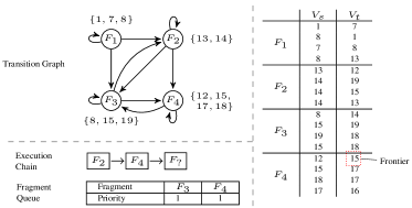
Figure 6: Example transition graph and auxiliary data structures.

We select the next fragment to read with the help of a light-weight, synopsis-based transition graph index (tgi). Conceptually, a tgi models a directed graph, where vertices denote fragments and edges represent transitions between them. A transition between two fragments $F_{1}$ and $F_{2}$ describes a path of length 2 with an edge $e_{1}=(u,v)$ in $F_{1}$ and an edge $e_{2}=(v,w)$ residing in $F_{2}$. If we read edge $e_{1}$ in fragment $F_{1}$ and proceed with the traversal afterwards, we have to read fragment $F_{2}$ as well, as it contains edges that extend the traversal path. A fragment has at most one fragment transition to any other fragment, including to itself. Since not every fragment has a transition to every other fragment in the transition graph, we only represent directed edges between fragments if there is a transition between them. In addition to fragment transitions, we store light-weight synopses representing the distinct values of each fragment. A fragment synopsis is stored as a compact bloom filter with bits set for all distinct values present in the fragment. Figure 6 depicts a transition graph with fragment size 4 for the edge column group on the right side. For example, there is a fragment transition $F_{2}\rightarrow F_{4}$ with a path $13\leadsto 12\leadsto 15$, i.e., $e_{1}=(13,12)$ in $F_{2}$ and $e_{2}=(12,15)$ in $F_{4}$. The fragment synopses are directly attached to the corresponding fragment, e.g., the fragment synopsis $\{13,14\}$ represents all distinct values in fragment $F_{2}$.

In addition to the tgi, we store query-specific runtime information about already processed fragments and fragment candidates in auxiliary data structures. We keep already processed fragments in a fragment execution chain and append to it whenever a new fragment has been selected for execution. Since we only choose a single fragment at a time, we queue all other generated fragment candidates in a priority-based fragment queue. To choose the next fragment for execution, we select the tail fragment of the execution chain and use the set of newly discovered vertices (the so-called frontiers) from the previous traversal round. Every vertex in the graph can only be a frontier vertex exactly once, i.e., when the vertex is first discovered.

1

2

Input :  Traversal configuration $\kappa=(S_{m},E_{\textit{a}},c,r,d)$.

Output :  Set of discovered vertices $R$.

3 begin

4       if $d$ is backward then

             $\textnormal{{swap}}(V_{\textit{s}}$,$V_{\textit{t}});$ // Adjust Column Handles

5            

6      

7      $D_{w}[0]\leftarrow S_{m}$;

8       $Frontiers\leftarrow S_{m}$;

9       $sFactor\leftarrow 1$;

10       $mFactor\leftarrow 1$;

11       while $\textnormal{{getNextFragment}}(Frontiers,F)$ do

12             $V_{\textit{s}}.\textnormal{{nWayScan}}(F,D_{w},E_{\textit{a}},sFactor,P)$;

13             $V_{\textit{t}}.\textnormal{{nWayMaterialize}}(P,mFactor,D_{\textit{w}},Frontiers)\;$ if $sFactor\leq r$ then  + + $sFactor$;

14             if $mFactor<r$ then  + + $mFactor$;

15            

16      $R\leftarrow\textnormal{{generateResult}}(c,r,D_{w})$;

17      

18

Algorithm 2 fi-traversal

For the tail fragment, we probe all adjacent fragment synopses with the frontier vertices. If an adjacent fragment matches, i.e. there is a transition between the tail and the adjacent fragment caused by one or more frontiers, the adjacent fragment is added to the fragment queue. If the fragment is already queued, we increase its priority. After updating the fragment queue, we remove the fragment with the highest priority and return it to the main traversal algorithm. If there are no frontier vertices, we immediately remove the fragment with the highest priority. If the fragment queue becomes empty, the traversal terminates.

Example. Let us consider an example traversal starting with vertex 13 as depicted in Figure 6. We start the traversal at fragment $F_{2}$ and emit the newly discovered vertex with id 12. During the fragment selection, we probe all adjacent fragments of $F_{2}$ (i.e., $F_{2}$, $F_{3}$, and $F_{4}$) with frontier vertex 12. Since fragment $F_{4}$ contains vertex 12 in its fragment synopsis, we select it as the next fragment to read. After processing fragment $F_{4}$, we emit frontier vertex 15 and select the next fragment to read. Since the probing generates two candidate fragments $F_{3}$ and $F_{4}$, we select one of them and continue the traversal.

After describing the principle workings of the fi-traversal algorithm, we sketch the algorithmic description in Algorithm 2. Initially, we pass a traversal configuration $\kappa$ with a vertex set $S_{m}$, an edge set $E_{a}$, a collection boundary $c$, a recursion boundary $r$, and a direction $d$ to the fi-traversal algorithm. It outputs a vertex set $R$ with visited vertices that have been discovered between $c$ and $r$. Since the execution of an fi-traversal is based on sequential reads of fragments, we parallelize the execution of the scan if necessary and materialize operations within a single column fragment. An fi-traversal runs in a series of iterations, where we process one fragment per iteration. At the beginning of each iteration, the algorithm getNextFragment receives a set of frontier vertices and returns the next fragment $F$ to read. A fragment contains the start and end position in the column and limits the scan to that range. Initially, we pass the set of start vertices as frontiers to getNextFragment. The body of the main loop performs a scan operation and a materialize operation (Lines 9–10). The scan takes the first sFactor working sets from the traversal iterations and returns matching edges in the corresponding position lists from the vector of position lists $P$. For example, an n-way scan with sFactor=2 probes the column with two vertex sets from two different traversal iterations and returns matching edges into two position lists. Subsequently, newly discovered adjacent vertices are materialized in a similar multi-way manner as in the scan operation. Depending on the mFactor, we read out the collected position lists and add adjacent vertices to the working sets from $D_{w}$. In addition, newly discovered vertices are added to the set of frontier vertices $Frontiers$. Once the recursion boundary is reached, the traversal reads and processes all remaining fragments from the fragment queue. If getNextFragment does not return any more fragments, the traversal terminates and generates the final result according to the given collection and recursion boundaries (Line 2).

Candidate Fragment Selection

1

2

Input :  Set of frontier vertices $Frontiers$.

Output :  Candidate fragment $F$ to read next.

3 begin

4       $F_{last}\leftarrow m\_chain.\textnormal{{getLast}}()$;

5       foreach outgoing edge $e=(F_{last},F_{cand})$ from $F$ do

6             foreach $v\in F$ do

7                   if $F_{cand}.\textnormal{{matches}}(v)\wedge\neg I.\textnormal{{hasKey}}(F_{cand},v)$ then

8                         $I.\textnormal{{insert}}(F_{cand},v)$;

9                         if $PQ.\textnormal{{hasKey}}(F_{cand})$ then

10                              $PQ.\textnormal{{increasePrio}}(F_{cand})$

11                        else $PQ.\textnormal{{insert}}(F)$;

12                        

13                  

14            

15      if $\neg PQ.\textnormal{{empty}}()$ then

16             $F\leftarrow PQ.\textnormal{{extractMin}}()$;

17             $m\_chain.\textnormal{{add}}(F)$;

18             return true;

19            

20      else return false;

21      

22

Algorithm 3 Procedure getNextFragment($Frontiers$,$F$)

Algorithm 3 describes in detail how to find the next fragment to read given a set of frontier vertices. It starts with the last processed fragment and probes adjacent fragments for matching vertices. For each adjacent fragment, we consult its fragment synopsis and compare the frontiers against it. If a frontier matches, we update the fragment queue accordingly. If the fragment is already in the queue, we increase its priority, otherwise we insert it. Further, we invalidate vertices in the synopses that triggered the candidate fragment selection. We keep invalidated vertices and their corresponding fragments in an invalidation list $I$ (Line 6). Finally, we return the fragment with the highest priority from the fragment queue and append it to the execution chain. Since the fragment synopses are implemented as compact bloom filters, false positive fragments can occur. However, a false positive does not harm the traversal functionally. There is a tradeoff between space consumption and execution time for the fragment synopses. We evaluate the effect of the size of a bloom filter in the experimental evaluation. Since the value distribution in fragments might vary, each bloom filter can have a different size depending on the number of distinct values present in the fragment.

Cost Model

The cost model of the fi-traversal is slightly more complex than for the ls-traversal since the calculation of the costs depends on a larger set of input parameters. The costs of an fi-traversal can be directly related to the number and the size of the accessed fragments. Hence, we can use the chain of read fragments $F_{p}$ to derive the cost of the fi-traversal. The overall cost is the accumulated cost of the reads for all accessed fragments in $F_{p}$. Consequently, the traversal cost is not directly dependent on the number of traversal iterations anymore. We define the cost $\mathcal{C}_{\text{FI}}$ of an fi-traversal in Equation 5 as follows.

$$\mathcal{C}_{\textsc{{fi}}}=\sum_{i=0}^{\min\{r,\tilde{\delta}\}}(1+p)(\bar{d}_{\text{out}})^{i}\cdot\xi\cdot\mathcal{C}_{e}$$ (5)

The cost depends on the average false positive rate $p$, the average vertex outdegree $\bar{d}_{\text{out}}$, and the fragment size $\xi$. The fi-traversal is bounded by the minimum of the recursion boundary $r$ and the estimated effective graph diameter $\tilde{\delta}$. The most important factors effecting the memory consumption of the tgi are the size and number of fragments. We can minimize the memory consumption of the tgi by grouping edges by source vertex (see edge clustering in Section 6). Then, each vertex with incoming and outgoing edges contributes exactly once to a single fragment transition. For equally-sized fragments, we have to choose a fragment size that is as large as the largest vertex out-degree. Therefore, we also propose to provide a heterogeneous fragment size distribution that is always larger than a predefined minimum fragment size. The upper size is determined automatically by the vertex out-degree. We discuss these configuration parameters and their performance implications for the fi-traversal in detail in the evaluation in Section 7.

6 Topology-Aware Clustering

The basic implementation of the ls-traversal algorithm does not rely on a particular ordering of the edges in the edge column group. However, to fully leverage the benefits of a main-memory storage engine, we can use data access patterns that provide a more efficient access to data placed in memory. Therefore, a physical reorganization of records is a common optimization strategy to reduce data access costs [6]. In the following, we describe two strategies to further reduce the overall execution time of the ls-traversal algorithm by maximizing the spatial locality of memory accesses to reduce the number of records to scan.

Type Clustering

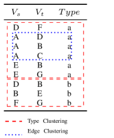
Figure 7: Clustered Edges.

Typically, real-world graph data sets are modeled with a widespread and diverse set of edge types that connect the vertices in the graph. Conceptually, an edge type describes a subgraph and can be interpreted as a separate layer or view on top of the original data graph. Such multi-relational graphs with multiple edge types are common in a variety of scenarios, such as product batch traceability, social network applications, or material flows graphs. For example, a product rating website might store different relationships between entity types rating, user, and product, such as rating relationships, product hierarchies, and user fellowships. To that end, traversal queries are specific with regard to which parts of the graph they refer to. We propose to arrange edges sharing the same type physically together, allowing a traversal query to operate directly on the subgraph instead of the entire original graph. Thus, a graph that comprises $n$ different edge types results in $n$ different subgraphs. A subgraph is associated with an area in the column that contains all edges forming the subgraph. Figure 7 illustrates an edge column group with two edge types. Here, a traversal query that refers to edges of type $b$ would only have to scan the corresponding subgraph. The portion of the column for edge type $b$ is indicated by the dashed lower rectangle. If the edge predicate contains a disjunctive condition, for example to traverse only over edges of type $a$ or $b$, the ls-traversal algorithm automatically splits the scan operation and unions the partial results thereafter.

Edge Clustering

The most fundamental component of a traversal operation is to retrieve the set of adjacent vertices for a given vertex. Therefore, an efficient traversal implementation must provide efficient access to adjacent vertices located in main memory. To achieve this, we introduce the notion of topological locality in a graph. Topological locality describes a concept for accessing all vertices adjacent to a given vertex $v\in V$. If a neighboring vertex of a vertex $v$ is accessed, it is likely that all other vertices adjacent of $v$ are accessed also.

We translate topological locality in a graph directly into spatial locality in memory by grouping edges based on their source vertex. Such an edge clustering increases spatial locality, i.e., all edges sharing the same source vertex are written consecutively in memory. Maximizing spatial locality for memory accesses results in a better last-level cache utilization and minimizes the amount of data to be loaded from main memory into the last-level cache of the processor [10]. Figure 7 sketches an example for vertex $A$. All edges having $A$ as source vertex are written consecutively into the edge column group. To that end, applying first clustering by type and then by edge extends the physical reorganization on a second level. Especially the materialization step of an ls-traversal algorithm benefits from an increased spatial locality while fetching adjacent vertices from the $V_{t}$ column (see Line 1 in Algorithm 1).

Besides the spatial locality, column decompression plays an important role in materializing adjacent vertices. Major in-memory database vendors rely on a two-level compression strategy. The first level is dictionary encoding, where a value is represented by its numerical value code from the dictionary and stored in a bit-packed, space-efficient data container. Here, a lightweight, but still notable decompression routine is used to reconstruct the actual value code. If adjacent vertices are not stored in a consecutive chunk of memory, the decompression routine might decompress unnecessary value codes. A similar behavior can be observed on the second level of compression, the value-based block compression. Edge clustering allows retrieving blocks of value codes that can be reconstructed efficiently by leveraging simd instructions.

7 Evaluation

We evaluate the ls-traversal and the fi-traversal on a diverse set of real-world graphs and for different types of graph queries. In the following, we describe the environmental setup and provide statistical information about the evaluated data sets. We present an extensive experimental evaluation of the memory consumption, execution time, cost model, and system-level comparison with two native graph management systems.

Environmental Setup and Data Sets

We have implemented graphite as a prototype in the context of the in-memory column-oriented sap hana database system. Graph data in sap hana is stored in two column groups, where each group has its own read-optimized main storage and write-optimized delta storage. Data manipulation operations exclusively modify the delta storage, which is periodically merged into the main storage. Deletions only invalidate records and affected records are being removed during the next merge process. Within the scope of this paper, we focus on read-only graphs, but argue that the proposed algorithms could be easily extended to support dynamic graphs as well (for example by treating the delta storage as a single fragment and by using general visibility data structures, such as a validity vector, to check for deletions). All values are dictionary-encoded allowing the traversal algorithms to operate on the value codes directly. Initially, we loaded the data sets into their corresponding vertex and edge column groups, and populate the tgi. We ran the experiments on a single server machine running SUSE Linux Enterprise Server 11 ($64\text{\,}\mathrm{bit}$) with Intel Xeon X5650 running at $2.67\text{\,}\mathrm{GHz}$, 6 cores, 12 threads, $12\text{\,}\mathrm{MB}$ L3 cache shared, and $48\text{\,}\mathrm{GB}$ RAM. For the ls-traversal we leverage full parallelization with 12 threads, for the fi-traversal we use 1 thread to scan a single fragment. To evaluate our approach on a wide range of different graph topologies, we selected six real-world graph data sets from the domains: social networks (or,tw,lj), citation networks (pa), autonomous system networks (sk), and road networks (cr). For each data set, we report the number of vertices $|V|$, the number of edges $|E|$, the average vertex outdegree $\bar{d}_{out}$, the maximum vertex outdegree $\max(d_{out})$, the estimated graph diameter $\tilde{\delta}$, and the raw size of the graph in Table 1.

ID	$|V|$	$|E|$	$\bar{d}_{out}$	$\max(d_{out})$	$\tilde{\delta}$	Size (MB)
cr	1.9 M	2.7 M	$2.8$	12	495.0	$143$
lj	4.8 M	68.5 M	$28.3$	635 K	6.5	$1\,617$
or	3.1 M	117.2 M	$76.3$	32 K	5.0	$3\,066$
pa	3.7 M	16.5 M	$8.7$	793	9.4	$397$
sk	1.7 M	11.1 M	$13.1$	35 K	5.9	$305$
tw	40.1 M	1.4 B	$36.4$	2.9 M	5.4	$32\,686$

Table 1: Evaluated data sets with their topology statistics.

All evaluated queries are of the form $\{\Set{s},\text{'\emph{*}'},k,k,\rightarrow\}$, where $s$ is a randomly selected start vertex, $*$ refers to a nonselective edge filter, and $k$ denotes the traversal depth. Without losing generality, we focus in the evaluation on traversal queries where the collection boundary is equal to the recursion boundary. Such traversal queries only return vertices first discovered in traversal iteration $k$. For the runtime analysis, we randomly selected start vertices for the traversal and report the median execution time over 50 runs. We decided to report the median since the execution highly varies for different start vertices.

We compare our ls-traversal and fi-traversal implementations against two join-based approaches (with and without secondary index support) in sap hana, the open-source version of Virtuoso Universal Server 7.1 [13], and the community edition of the native graph database management system Neo4j 2.1.3 [3]. For the experiments we prepared and configured the evaluated systems as follows:

SAP HANA

We populated the data sets into two columnar tables, one for vertices and one for the edges. For the indexed join, we created a secondary index on the source vertex column.

Virtuoso

Since Virtuoso is an RDF store, we transformed all data sets into RDF triples of the form <source_id> <edge_type> <target_id> and use sparql property paths to emulate a breadth-first traversal. We increased the number of buffers (NumberOfBuffers) and maximum dirty buffers (MaxDirtyBuffers) as recommended.

Neo4j

We configured the object caches of Neo4j so that the data set fits entirely into memory. We warmed up the object cache by running randomly 10000 traversal queries against the database instance. To run the experiments, we used Neo4j’s declarative query lanuage Cypher and created an additional index on the vertex identifier attribute.

TGI Memory Consumption

In this experiment we study the effect of various algorithm parameter configurations on the memory consumption of the tgi. We populated tgi instances for clustered physical edge ordering with different fragment sizes and false positive rates, and present the results in Figure 8. To evaluate the impact of the fragment size $\xi$, we construct the tgi for different fragment sizes $2^{6},\ldots,2^{16}$ and a fixed average false positive rate of $1\%$. We analyze the effect of the average false positive rate for a representative fragment size $\xi=512$ and construct fragment synopses based on an average false positive rate $p$ selected from $\{1\%,5\%,10\%,20\%\}$.

The size of the tgi is directly related to the total number of edges of the original input graph. For fragment size $\xi=1024$, the tgi consumes only about $10\%$ of the size of the input graph. For $\xi=1024$, the tgi of data set tw has the highest memory consumption with about $2.09\text{\,}\mathrm{GB}$ (about 8.4% of the raw size of the graph) and data set cr the lowest memory consumption (about 8.8% of the raw size of the graph). For disabled clustering by edge, the memory consumption of the tgi can grow up to a factor of 10 of the original graph. This makes the unclustered variant of the fi-traversal impractical for a productive system as it occupies up to two orders of magnitude the memory of the clustered variant.

Impact of Fragment Size

For all evaluated data sets, the memory footprint decreases for increasing fragment sizes. A larger fragment size leads to a smaller number of vertices in the tgi and consequently to fewer possible transitions between them. Although larger fragments cause a denser tgi topology, the total number of fragment transitions is much lower than for smaller fragments. For input graphs with a larger average vertex outdegree, the memory overhead can be reduced for $\xi=2^{16}$ to up to $13\%$ of the memory overhead for $\xi=2^{6}$. For very sparse graphs, such as cr, the tgi consumes about $37\%$ of the memory for $\xi=2^{16}$ compared to $\xi=2^{6}$. Consequently, the sparser the input graph is, the lower is the impact of the fragment size on the total memory consumption of the tgi.

Impact of False Positive Rate

We store fragment synopses in space-efficient bloom filter data structures, where each fragment synopsis occupies as much memory as needed to fulfill the predefined false positive rate. A smaller false positive rate causes the fi-traversal to access more fragments, but reduces the memory footprint of the tgi. We show the memory overhead for different false positive rates in Figure 8. For data set pa, a false positive rate of $20\%$ leads to a memory footprint decrease of $13\%$ compared to a false positive rate of $1\%$. In contrast, data set cr reached a memory footprint decrease of almost $50\%$ for $p=20\%$ compared to $p=1\%$.

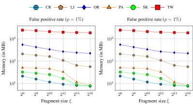
Figure 8: tgi memory consumption for different false positive rates and fragment sizes.

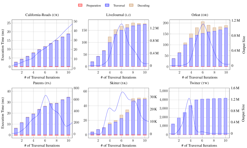
Figure 9: Execution time and output size of ls-traversal for different queries and data sets.

Runtime Analysis

Figure 9 presents the runtime results of the ls-traversal for all data sets and with different traversal queries. We report average execution times of the three traversal phases preparation, traversal, and decoding as well as average output sizes. In general, the traversal phase dominates the overall execution time of the traversal operator and consumes up to 95% of the total runtime. The runtime of the preparation phase is only about 5% of the overall execution time and is independent from the number of traversal iterations. The preparation phase only evaluates the edge predicate and processes the start vertices. The decoding phase highly depends on the size of the vertex output set as it translates for each vertex the value code back into the corresponding vertex identifier. For the data set sk, we can see the effect of the output size on the runtime spent for the decoding. The output size of the traversal steadily grows until the traversal reaches the effective diameter. Consequently, only very few traversals reach a larger traversal depth than the effective diameter. The ls-traversal scales almost linearly with increasing number of traversal iterations as the full column scan takes about the same time to complete independent of the traversal iteration.

Figure 10 presents an in-depth comparison of ls-traversal and fi-traversal on all data sets for fragment sizes $\{2^{7},\ldots,2^{10}\}$. Larger fragment sizes resulted in higher execution times and are therefore omitted in the results. For all evaluated data sets, ls-traversal shows a linear runtime behavior for an increasing number of traversal iterations. For the data set pa, the runtime steadily increases until the ls-traversal reaches the effective diameter. After the traversal query reached the effective diameter, the plot flattens for longer traversal queries. In comparison, the data plots of the fi-traversal grow much faster for an increasing number of traversal iterations. For short traversals with a low number of traversal iterations, the fi-traversal outperforms the ls-traversal by up to two orders of magnitude. This can be explained by the more fine-granular graph access pattern of the fi-traversal. Especially the first traversal iterations process only very small parts of the whole graph and a fine-granular fragment access clearly outperforms a full column scan. For a large working set, potentially many fragments have to be accessed which in turn is hard to predict and prefetched by the hardware. If large parts of the graph are accessed, a single full column scan is superior compared to many small fragment scans. The break-even point when the fi-traversal outperforms the ls-traversal depends on the graph topology and the given traversal query. From the results we can conclude that short traversal queries clearly favor the fi-traversal over the ls-traversal. Even for short traversal queries, both data sets produce large intermediate results due to the power-law distribution of vertex outdegrees making the fi-traversal less effective. For 4 out of 6 data sets, the fi-traversal outperforms the ls-traversal for traversal queries with $r\leq 5$. The fragment size has a severe impact on the overall execution performance of the fi-traversal. For data set cr, the fragment size does not only effect the total runtime, but also increases the range of traversal queries, where the fi-traversal outperforms the ls-traversal. For example, a traversal query with traversal depth 14 on data set cr consumes only about $26\%$ of the runtime than for $\xi=2^{10}$ for a fragment size $\xi=2^{7}$. In general, we can conclude that fi-traversal is superior to ls-traversal for very sparse graphs or for short traversal queries.

Figure 11 depicts the slowdown factors for all data sets with different fragment sizes $\{2^{6},\ldots,2^{16}\}$. To compute the slowdown factor, we use the data point for the smallest fragment size/false positive rate as baseline and relate all other results to this baseline. Further, we analyze the effect of the false positive rate on the query runtime. Without losing generality, we conduct all experiments on a representative query of the form $\{\Set{s},\text{'\emph{*}'},3,3,\rightarrow\}$. In general, the fi-traversal with enabled edge clustering finished the execution on average about 3.5 times faster than for the unclustered variant. If the graph is not clustered by edge, the probability of a transition to another fragment is significantly higher due to a higher number of distinct values in the fragment. For enabled edge clustering, the maximum number of possible transitions is bounded by the number of vertices in the graph. For all data sets, smaller fragment sizes close to the expected average vertex outdegree are more beneficial with respect to execution performance than larger ones. Although one could specify a fragment size that is very small or even close to 1, the memory overhead would be prohibitively high. Therefore, we limit the minimum fragment size to be connected to the vertex outdegree.
A larger false positive rate increases the memory consumption of the tgi, but speeds up the runtime of the fi-traversal. If the false positive rate is too large, many fragments are read although they do not contribute to the traversal query result.

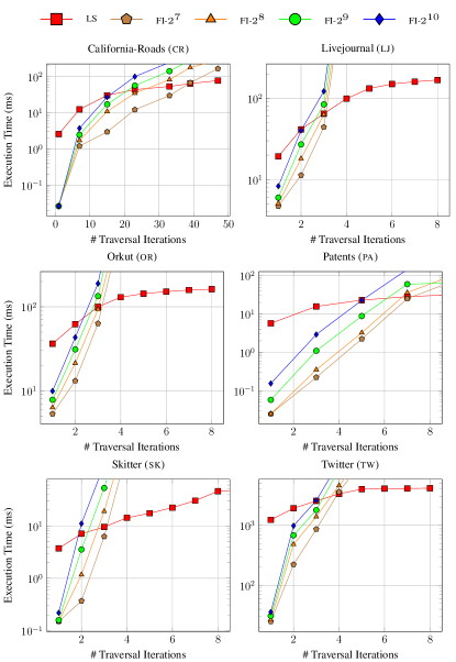
Figure 10: Comparison of ls-traversal and fi-traversal for different queries and data sets.

Figure 11: Execution time of fi-traversal for $\{\Set{s},\text{'\emph{*}'},3,3,\rightarrow\}$.

Impact of Edge Predicates

We study the effect of edge predicates on the query performance of the ls-traversal and the fi-traversal in Figure 12. An edge predicate selects a subgraph of the entire data graph and limits the traversal to a subset of active edges. We generated edge weights following a zipfian distribution with $s=2$ and assigned them randomly to the edges. For a selectivity of $25\%$, i.e., an edge predicate that selects only $25\%$ of all edges leads for the ls-traversal to a speedup of 3. We observed that an edge predicate with a low selectivity drastically reduces the size of intermediate and final output results. Since the ls-traversal is a scan-based traversal algorithm, it still has to scan the entire column for each traversal iteration. In contrast, the fi-traversal reaches a speedup of up to factor 6 for a selectivity of $25\%$. If the selectivity is low, more fragments can be pruned during the traversal and cause the doubled speedup compared to the ls-traversal .

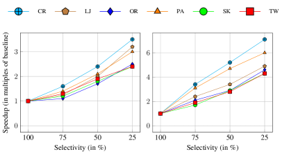
Figure 12: Speedup in multiples of baseline for different edge predicate selectivities with query $\{\Set{s},\text{'\emph{*}'},3,3,\rightarrow\}$. The baseline is a traversal query without edge predicate, i.e., a traversal on the entire graph.

System-Level Benchmarks

We compared our two traversal implementations with a purely relational self-join-based approach (with and without secondary index support), Neo4j, and Virtuoso 7.0. For the join-based traversal, we use the same data layout as for graphite and leverage the columnar relational engine of sap hana. We present our results in Figure 13. For short traversals of 1–3 hops, our fi-traversal is competitive with native graph implementations from Neo4j and Virtuoso. For data sets pa, sk, and cr fi-traversal outperforms all evaluated systems by up to an order of magnitude.

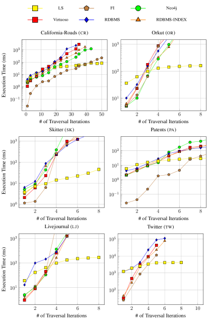
Figure 13: System-level benchmarks of ls-traversal, fi-traversal, virtuoso, neo4j, and a self-join-based approach (with and without secondary index support). Since the execution times highly vary for different start vertices, we report median execution times. We were not able to run experiments for the Twitter data set on Neo4j due to data loading issues.

Cost Model Evaluation

To verify our cost model function, we applied regression analysis. We use the coefficient of determination denoted $R^{2}$ to evaluate the quality of our fi-traversal cost model. The coefficient of determination has a value range of $-1\leq|R^{2}|\leq 1$. A value of $|R^{2}|$ close to 1 indicates a good fit of the proposed cost model function with the manually collected data points. We compare the manually collected data of the number of accessed edges against the results of the cost function. For each data set, we performed a set of traversal queries with a recursion boundary ranging from 1 to 10. We achieved the best result with an average $R^{2}=0.92$ for data set cr, respectively. For the data set ep, we achieved $R^{2}=0.78$. In general, graphs with a power-law vertex outdegree distribution caused our cost function to underestimate the costs of the fi-traversal. This underestimation can be explained by the method used to describe the vertex outdegree distribution. We use the average vertex outdegree $\bar{d}_{\text{out}}$ to estimate the expected number of neighbors for a single vertex. If the traversal discovers a vertex with a considerably larger vertex outdegree, the cost function underestimates the access costs. Additionally, the traversal depth is estimated as the minimum of the recursion boundary and the diameter of the graph. However, traversal queries that terminate before they reach the recursion boundary, are not appropriately reflected in the cost function. We believe that additional information about the outdegree distribution and the distribution of path lengths is required to obtain a more accurate estimation from the cost function.

8 Related Work

Graph Traversal Algorithms

Graph traversals are one of the most important and fundamental building blocks of graph algorithms, such as finding shortest paths, computing the maximum flow, and identifying strongly connected components. Increasing graph data sizes and the proliferation of parallelism on different hardware levels as well as heterogeneous processor environments encouraged researchers to revise the well-known breadth-first graph traversal and to propose novel techniques to run graph traversals on high-end computers with large numbers of cores and different types of processors on a single machine. A large body of research has been conducted on efficient parallel graph traversals, lately even leveraging co-processors to speed up graph processing on large data graphs [17]. State-of-the-art parallel graph traversals operate with a level-synchronous strategy and parallelize the work to be done at each level. However, all parallel graph traversal implementations rely on sophisticated data structures that are tailored to the graph traversal algorithm. Such an algorithm-dependent data structure is not applicable in our case since we are using the traversal operator in an rdbms on top of a common storage engine without copying data into separate data structures. As one of our strongest advantages, we do not require the graph data to be copied from possibly already existing legacy relational tables into algorithm-specific data structures. Replicating data into separate data structures wastes memory and also adds a considerable maintenance overhead. Chhugani et al. study scalable breadth-first traversal algorithms on modern hardware with multi-socket, multi-core processor architectures [12, 27]. They achieved an impressive performance by tuning the data structures and the traversal algorithm to the underlying hardware. In contrast to our approach, they only consider a single implementation of graph traversals for any graph topology and types of graph traversal queries. Graph traversals in distributed memory recently gained more attention and resulted in the development of sophisticated data partitioning schemes for distributed graph traversals [11, 26].

Graph Processing on Column Stores

Column stores have shown great potential for storing and querying wide and sparse data [4]. These considerations brought up research projects that aimed to provide efficient access to rdf [7] and xmldata [30] kept in a column store. However, none of them covered the design and implementation of a native graph traversal operator that leverages advantages of columnar data structures and exploits knowledge about the graph topology to speed up the graph traversal execution.

Distributed Graph Engines

The demand to efficiently process real-world billion-scale graphs triggered the development of a variety of distributed graph processing systems [15, 18, 21, 22]. GBase is a distributed graph engine based on MapReduce and relies on distributed matrix-vector multiplications [18]. The vertex-centric programming model, as proposed by [22], has been an area of active research and has been implemented in GraphLab [21] and PowerGraph [15] among others. Although distributed graph engines show good scalability for billion-scale graphs, we see the following disadvantages making them not applicable in our scenarios: (1) Business data from enterprise-critical applications is still mainly stored in rdbms and cannot be easily replicated to external graph processing engines; (2) typically, graph engines cannot cope with cross-data-model operations (e.g., combining text, graph, and spatial); (3) distributed graph engines rely on sophisticated graph partitioning algorithms that do not scale well to large graphs and are hard to maintain for dynamic graphs; and (4) they do not provide transactional guarantees.

Single-Machine Graph Engines

An interesting alternative to distributed graph engines has been introduced by Kyrola et al. [19] and conceptually extended by Han et al. [16]. GraphChi is a disk-based graph engine on a single machine that exploits parallel sliding windows and sharding to efficiently process billion-scale graphs from disk [19]. To minimize I/O overhead, they apply a technique similar to edge clustering to improve disk access and maximize data locality on disk. The lack of support for attributes on vertices and edges and dynamic graphs resulted in GraphChi-DB, a recent extension of GraphChi [20]. Interestingly, they also use a vertically partitioned layout to represent attributes on vertices and edges. In contrast to GraphChi we run graphite not as a standalone graph engine, but as part of a graph runtime stack on a common relational storage engine in an rdbms. Since our targeted scenarios run on main-memory rdbms, graphite can operate completely in memory and aims at maximizing cpu cache locality. Similar to GraphChi is TurboGraph, a single-machine disk-based graph processing engine using solid state disks (ssd) to store and process large graphs [16]. They use a vertically partitioned layout on ssd to store vertex attributes. However, we do see two major drawbacks compared to our approach: (1) GraphChi and TurboGraph are efficient single-machine graph engines, but do not provide transactional access to the data; and (2) graph data has to be available upfront in a specific data format on disk. To be applicable for business data stored in rdbms, the data has to be exported and transformed into a file format that can be consumed by the system.

Graph Databases

A different direction is followed by graph databases, such as Neo4j [3], Sparksee [23], and InfiniteGraph [2]. While Neo4j relies on a disk-based storage accelerated by buffer pools to store recently accessed parts of the graph, Sparksee allows manipulating and querying the graph in memory. The Sparksee internal data structures rely on efficient bitmaps, which represent the set of vertices and edges describing the graph [23]. All graph databases are specialized engines that can perform graph-oriented processing efficiently, but always require loading possibly relational business data in advance from other data sources. On the contrary, our approach can directly operate on the relational business data without having to copy it to a dedicated database engine. Moreover, the combination of relational operations and graph operations can be handled efficiently by a single database engine.

Graph Processing in rdbms

Although graph databases are a rather new research field, path traversals in relational databases with the help of recursive queries have been in the focus of research for more than 20 years now [8]. There have been proposals for extending relational query languages with support for recursion in the past and even the SQL:1999 standard offers recursive common table expressions. However, commercial database vendors often provide their own proprietary functionality, if they do at all. Gao et al. leverage recent extensions to the SQL standard, such as window functions and merge statements, to implement algorithms for shortest path discovery on relational tables [14]. Unlike our approach, they are reusing existing relational operators and the relational query optimizer to create an optimal execution plan. However, when ignoring graph-specific statistics, the optimizer is likely to select a suboptimal execution plan. Magic-set transformations are a query rewrite technique for optimizing recursive and non-recursive queries, which was originally devised for Datalog [9] and has been extended for SQL [25]. Since graph traversals can be expressed as recursive database queries, the magic-sets transformation could also be applied to them. However, instead of proposing an optimization strategy for relational execution plans, we approach the problem with a dedicated plan operator.

9 Conclusion

We presented graphite, a modular and versatile graph traversal framework for main-memory rdbms. As part of graphite, we presented two different specialized traversal implementations named ls-traversal and fi-traversal to support a wide range of different graph topologies and varying graph traversal queries most efficiently. graphite is extensible and other graph traversal strategies, such as depth-first based traversals, could be integrated as well. We derived a basic cost model of two traversal implementations and experimentally showed that it can assist a query optimizer to select the optimal traversal implementation. The fi-traversal outperforms the ls-traversal for graphs with a low density and short traversal queries by up to two orders of magnitude. In contrast, the ls-traversal performs significantly better than the fi-traversal, if the graph is dense or the query traverses a large fraction of the whole graph. Our experimental results illustrate the need for a graph traversal framework with an accompanied set of traversal operator implementations. Finally, we show that, despite popular belief, graph traversals can be efficiently implemented in rdbms on a common relational storage engine and are competitive with those of native graph management systems.

References

- [1] Apache Giraph project website. \urlhttp://www.giraph.apache.org/.
- [2] InfiniteGraph project website. \urlhttp://objectivity.com/INFINITEGRAPH.
- [3] Neo4j project website. \urlhttp://neo4j.org/.
- [4] D. Abadi. Column Stores for Wide and Sparse Data. In Proc. CIDR’07, pages 292–297, 2007.
- [5] D. Abadi, R. Agrawal, A. Ailamaki, M. Balazinska, P. A. Bernstein, M. J. Carey, S. Chaudhuri, J. Dean, A. Doan, M. J. Franklin, et al. The beckman report on database research. ACM SIGMOD Record, 43(3):61–70, 2014.
- [6] D. Abadi, S. Madden, and M. Ferreira. Integrating Compression and Execution in Column-oriented Database Systems. In Proc. SIGMOD’06, pages 671–682, 2006.
- [7] D. Abadi, A. Marcus, S. R. Madden, and K. Hollenbach. Scalable Semantic Web Data Management Using Vertical Partitioning. In Proc. VLDB’07, pages 411–422, 2007.
- [8] R. Agrawal. Alpha: An Extension of Relational Algebra to Express a Class of Recursive Queries. 14(7):879–885, 1988.
- [9] F. Bancilhon, D. Maier, Y. Sagiv, and J. D. Ullman. Magic Sets and Other Strange Ways to Implement Logic Programs. In Proc. PODS’86, pages 1–15, 1986.
- [10] P. Boncz, S. Manegold, and M. Kersten. Database Architecture Optimized for the New Bottleneck: Memory Access. In Proc. VLDB’99, pages 54–65, 1999.
- [11] A. Buluç and K. Madduri. Parallel Breadth-First Search on Distributed Memory Systems. In Proc. SC’11, pages 1–12, 2011.
- [12] J. Chhugani, N. Satish, C. Kim, J. Sewall, and P. Dubey. Fast and Efficient Graph Traversal Algorithm for CPUs: Maximizing Single-Node Efficiency. In Proc. IPDPS’12, pages 378–389, 2012.
- [13] O. Erling. Virtuoso, a Hybrid RDBMS/Graph Column Store. IEEE Data Eng. Bull., 35:3–8, 2012.
- [14] J. Gao, R. Jin, J. Zhou, J. X. Yu, X. Jiang, and T. Wang. Relational Approach for Shortest Path Discovery over Large Graphs. Proc. VLDB Endow., 5(4):358–369, Dec. 2011.
- [15] J. E. Gonzalez, Y. Low, H. Gu, D. Bickson, and C. Guestrin. PowerGraph: Distributed Graph-parallel Computation on Natural Graphs. In Proc. OSDI’12, pages 17–30, 2012.
- [16] W.-S. Han, S. Lee, K. Park, J.-H. Lee, M.-S. Kim, J. Kim, and H. Yu. TurboGraph: A Fast Parallel Graph Engine Handling Billion-scale Graphs in a Single PC. In Proc. KDD’13, pages 77–85, 2013.
- [17] S. Hong, T. Oguntebi, and K. Olukotun. Efficient Parallel Graph Exploration on Multi-Core CPU and GPU. In Proc. PACT’11, pages 78–88, 2011.
- [18] U. Kang, H. Tong, J. Sun, C.-Y. Lin, and C. Faloutsos. GBASE: A Scalable and General Graph Management System. In Proc. KDD’11, pages 1091–1099, 2011.
- [19] A. Kyrola, G. Blelloch, and C. Guestrin. GraphChi: Large-scale Graph Computation on Just a PC. In Proc. OSDI’12, pages 31–46, 2012.
- [20] A. Kyrola and C. Guestrin. GraphChi-DB: Simple Design for a Scalable Graph Database System - on Just a PC. CoRR, abs/1403.0701, 2014.
- [21] Y. Low, D. Bickson, J. Gonzalez, C. Guestrin, A. Kyrola, and J. M. Hellerstein. Distributed GraphLab: A Framework for Machine Learning and Data Mining in the Cloud. Proc. VLDB Endow., 5(8):716–727, Apr. 2012.
- [22] G. Malewicz, M. H. Austern, A. J. Bik, J. C. Dehnert, I. Horn, N. Leiser, and G. Czajkowski. Pregel: A System for Large-scale Graph Processing. In Proc. SIGMOD’10, pages 135–146, 2010.
- [23] N. Martínez-Bazan, M. A. Águila Lorente, V. Muntés-Mulero, D. Dominguez-Sal, S. Gómez-Villamor, and J.-L. Larriba-Pey. Efficient graph management based on bitmap indices. In Proc. IDEAS’12, pages 110–119, 2012.
- [24] N. Martínez-Bazan, V. Muntés-Mulero, S. Gómez-Villamor, J. Nin, M.-A. Sánchez-Martínez, and J.-L. Larriba-Pey. DEX: High-Performance Exploration on Large Graphs for Information Retrieval. In Proc. CIKM’07, pages 573–582, 2007.
- [25] I. S. Mumick and H. Pirahesh. Implementation of Magic-sets in a Relational Database System. In Proc. SIGMOD’94, pages 103–114, 1994.
- [26] R. Pearce, M. Gokhale, and N. M. Amato. Multithreaded Asynchronous Graph Traversal for In-Memory and Semi-External Memory. In Proc. SC’10, pages 1–11, 2010.
- [27] V. Prabhakaran, M. Wu, X. Weng, F. McSherry, L. Zhou, and M. Haridasan. Managing Large Graphs on Multi-cores with Graph Awareness. In Proc. USENIX ATC’12, pages 41–52, 2012.
- [28] M. A. Rodriguez and P. Neubauer. Constructions from Dots and Lines. Bulletin of the American Society for Information Science and Technology, 36(6):35–41, 2010.
- [29] M. A. Rodriguez and P. Neubauer. A Path Algebra for Multi-Relational Graphs. In Proc. ICDEW’11, pages 128–131, 2011.
- [30] J. T. Teubner. Pathfinder: XQuery Compilation Techniques for Relational Database Targets. PhD thesis, TUM, 2006. \urlhttp://www-db.in.tum.de/ teubnerj/publications/diss.pdf.