3D Source Localization and Polarimetry using High Numerical Aperture Imaging with Rotating PSF

Abstract

Rotating-PSF imaging via spiral phase engineering can localize point sources over large focal depths in a snapshot mode. This letter presents a full vector-field analysis of the rotating-PSF imager that quantifies the PSF signature of the polarization state of the imaging light. For sufficiently high image-space numerical apertures, there can be significant wave-polarization dependent contributions to the overall PSF, which would allow one to jointly localize and sense the polarization state of light emitted by point sources in a 3D field.

OCIS Codes: (110.5405) Polarimetric imaging; (110.6880) Three-dimensional image acquisition; (110.7348) Wavefront encoding; (110.1758) Computational imaging; (100.2960) Image analysis.

The orbital angular momentum (OAM) of light can encode the axial position of a source point via the rotation of its image, the so-called point spread function (PSF). As one of us has shown SP13 , an annular spiral phase structure in the circular pupil of an imager yields a PSF that, as a coherent superposition of non-diffracting Bessel beams, rotates about the Gaussian image point nearly rigidly as the source is displaced axially from the Gaussian image plane (GIP). In its superior depth of field and PSF compactness, this system vastly improves upon previous rotating-PSF imagers PP08 ; LLBM11 ; GDQDP12 , all of which combine fully diffracting Gauss-Laguerre vortex modes in the pupil. The angle of the PSF rotation, being proportional to the axial displacement, or defocus, of the source from the GIP, thus enables one to localize a source fully in all three dimensions.

For rotating-PSF imaging with a high image-space numerical aperture (NA), we must include the transversality of the electromagnetic field via a vector-field analysis MM92 ; JK06 ; THYH13 . Such an analysis accounts properly for wave polarization, related fundamentally to the spin angular momentum (SAM) of the photon, and is thus needed to describe polarization-dependent modifications of the rotating PSF. This is a subtle effect, as we shall see, one that is best seen via the nonvanishing longitudinal field components of the imaging beam Jackson99 . One expects SAM to modify the rotating PSF amplitude from its OAM-only form by an amount proportional to the product of the NA and that contributed by one unit of angular momentum when the light is completely circularly polarized, with still subtler modifications for more general wave polarization states. It is this modification and its exploitation for snapshot 3D polarimetric imaging that is the subject of the present letter.

The spiral pupil phase structure which yields a compact PSF that rotates without much distortion is

$$\Psi(u,\phi_{u})=\left\{f_{l}(\phi_{u})\,\Bigg{|}\,\sqrt{l-1\over L}\leq u<\sqrt{l\over L},\ l=1,\ldots,L\right\},$$ (1)

where $u=\rho/R$ is the normalized radial coordinate in the circular pupil of radius $R$ and $\phi_{u}$ is the azimuthal angle. The simplest form for the spiral phase $f_{l}(\phi_{u})$ in the $l$th annular zone is, up to an unimportant additive constant, $\pm l\phi_{u}$ SP13 , for which a single-lobe PSF results. However, any spiral phase distribution with an integral winding number in each zone that changes by a fixed step from one zone to the next will do, with the number of lobes of the resulting PSF being equal to the step size of the phase winding number.

Consider a point electric dipole source located at the origin, with dipole moment $\vec{p}$ oscillating at angular frequency $\omega$ in a plane transverse to the $z$ axis,

$$\vec{p}(t)=(p_{+}\hat{e}_{+}+p_{-}\hat{e}_{-})\exp(-i\omega t),$$ (2)

where $\hat{e}_{\pm}$ are the circular-polarization (CP) unit basis vectors, $\hat{e}_{\pm}=(\hat{x}\pm i\hat{y})/\sqrt{2}$. The electric field radiated by the dipole at location $\vec{r}$ in the radiation zone has the form Jackson99

$$\vec{E}(\vec{r},t)={k^{2}\over 4\pi\epsilon_{0}r}[\vec{p}-(\vec{p}\cdot\hat{n})\hat{n}]\,\exp(ikr-i\omega t),$$ (3)

where $k=\omega/c$ is the propagation constant of radiation and $\hat{n}=\vec{r}/r$ is the unit observation vector. In view of (2) and since

$$\hat{n}={1\over\sqrt{2}}\sin\theta\left(e^{i\phi}\hat{e}_{-}+e^{-i\phi}\hat{e}_{+}\right)+\cos\theta\hat{z},$$ (4)

up to the linear order in the paraxial angle $\theta$, the electric field (3) takes the form

$$\vec{E}(\vec{r})={k^{2}\over 4\pi\epsilon_{0}r} \Biggl{[}p_{+}\hat{e}_{+}+p_{-}\hat{e}_{-}$$

$$-{\theta\over\sqrt{2}}(p_{+}e^{i\phi}+p_{-}e^{-i\phi})\hat{z}\Biggr{]}\exp(ikr),$$ (5)

where we have omitted the time dependence of the field for the sake of brevity. It is the longitudinal ($z$) component of the electric field in (3D Source Localization and Polarimetry using High Numerical Aperture Imaging with Rotating PSF) that yields a helical component to the Poynting vector responsible for the AM of the radiation field.

In the thin-lens and paraxial (Fresnel) propagation limits that we assume here, in passing through the lens aperture with the spiral phase structure (1), the transverse field, $\vec{E}_{>}^{(T)}(\vec{r},t)$, acquires the phase shift, $-kR^{2}u^{2}/(2f)-\Psi(u,\phi)$, where $f$ is the lens focal length. Just past the aperture, it thus has the form

$$\vec{E}_{>}^{(T)}(\vec{r})={k^{2}\over 4\pi\epsilon_{0}z_{0}}\left[p_{+}\hat{e}_{+}+p_{-}\hat{e}_{-}\right]\exp[i\Phi(\vec{u})],$$ (6)

where $r$ has been replaced by the axial source distance, $z_{O}$, from the lens pupil in the denominator but by its more accurate, paraxial form, $z_{O}+R^{2}u^{2}/(2z_{O})$, inside the phase factor $\exp(ikr)$ of (3D Source Localization and Polarimetry using High Numerical Aperture Imaging with Rotating PSF). As a result, the spatial phase function in the pupil has the form,

$$\Phi(\vec{u})=kz_{O}+{kR^{2}\over 2}\left({1\over z_{O}}-{1\over f}\right)u^{2}-\Psi(\vec{u}).$$ (7)

For lens apertures that are large compared to the wavelength, the transverse components of the electric field vector diffract approximately via the scalar Fresnel-diffraction formula Goodman96 . As such, $\vec{E}^{(T)}(\vec{r}_{I})$ at a distance $z_{I}$ from the lens aperture is the sum of its two CP components,

$$\vec{E}^{(T)}(\vec{r}_{I})=\vec{E}^{(T)}_{+}(\vec{r}_{I})+\vec{E}^{(T)}_{-}(\vec{r}_{I}),$$ (8)

that may be expressed as

$$\vec{E}^{(T)}_{\pm}(\vec{r}_{I})= {k^{2}R^{2}e^{ik(z_{O}+z_{I})}\over 4\pi\epsilon_{0}z_{O}i\lambda z_{I}}p_{\pm}\hat{e}_{\pm}$$

$$\times\int P(u)e^{i\zeta u^{2}-i\Psi(\vec{u})-i2\pi\vec{u}\cdot\vec{s}}d^{2}u.$$ (9)

Here $P(u)$ is the aperture function that is equal to 1 inside the aperture, i.e., for $u<1$, and 0 outside, and $\zeta$ is the defocus phase at the edge of the pupil, defined as

$$\zeta={kR^{2}\over 2}\left({1\over z_{O}}+{1\over z_{I}}-{1\over f}\right)={kR^{2}\over 2}{\delta z_{O}\over z_{O}(z_{O}+\delta z_{O})},$$ (10)

where $\delta z_{O}$ is the distance of the source from the plane of best paraxial focus for which the thin-lens equation holds. In (3D Source Localization and Polarimetry using High Numerical Aperture Imaging with Rotating PSF), we have scaled the transverse image-plane position vector, $\vec{\rho}_{I}$, by dividing it by the characteristic size of the Airy diffraction spot, $\lambda z_{I}/R$, to arrive at $\vec{s}=\vec{\rho}_{I}/(\lambda z_{I}/R)$. For brevity we have suppressed here and in the expressions to follow the space-dependent phase factor $\exp[ik\rho_{I}^{2}/(2z_{I})]$.

A quarter-wave of defocus phase, i.e. $\zeta=\pm\pi/2$, was defined by Rayleigh Mahajan91 to correspond to the characteristic depth of field (DOF) for a clear-aperture imager. By contrast, an $L$-zone rotating-PSF imager has a DOF that corresponds to $\pm L/2$ waves of defocus phase SP13 , which is $2L$ times as large as the Rayleigh DOF.

From expression (3D Source Localization and Polarimetry using High Numerical Aperture Imaging with Rotating PSF) for the transverse field components, we can construct the corresponding longitudinal components, $E^{(z)}_{\pm}$, in the image plane by imposing the transversality of the full field, $\vec{\nabla}\cdot\vec{E}=0$. For paraxial propagation, $\partial E^{(z)}_{\pm}/\partial z$ may be replaced approximately by $ikE^{(z)}_{\pm}$, so the transversality condition is equivalent to $ikE^{(z)}_{\pm}=-\vec{\nabla}^{(T)}\cdot\vec{E}^{(T)}_{\pm}$, which gives

$$E^{(z)}_{\pm}(\vec{s})= {i\over k}\vec{\nabla}^{(T)}\cdot\vec{E}^{(T)}_{\pm}(\vec{r}_{I})$$

$$= {-ik^{3}R^{3}e^{ik(z_{0}+z_{I})}\over 8\pi^{2}\epsilon_{0}z_{0}z_{I}^{2}}p_{\pm}$$

$$\times\int P(u)\hat{e}_{\pm}\cdot\vec{u}\,e^{i\zeta u^{2}-i\Psi(\vec{u})-i2\pi\vec{u}\cdot\vec{s}}d^{2}u$$

$$= {-ik^{3}R^{3}e^{ik(z_{0}+z_{I})}\over 8\sqrt{2}\pi^{2}\epsilon_{0}z_{0}z_{I}^{2}}p_{\pm}$$

$$\times\int P(u)\,u\,e^{i\zeta u^{2}-i\Psi(\vec{u})\pm i\phi_{u}-i2\pi\vec{u}\cdot\vec{s}}d^{2}u,$$ (11)

where we used the identity $\hat{e}_{\pm}\cdot\vec{u}=u\exp(\pm i\phi_{u})/\sqrt{2}$ to reach the final expression. We also ignored a negligibly small contribution to the transverse divergence in (3D Source Localization and Polarimetry using High Numerical Aperture Imaging with Rotating PSF) from the phase factor $\exp[ik\rho_{I}^{2}/(2z_{I})]$ that was omitted in (3D Source Localization and Polarimetry using High Numerical Aperture Imaging with Rotating PSF). As expected, it is the longitudinal components of the electromagnetic field that clearly exhibit the SAM for the two CP components via the phase factors $\exp(\pm i\phi_{u})$ in (3D Source Localization and Polarimetry using High Numerical Aperture Imaging with Rotating PSF).

From the first expression in (3D Source Localization and Polarimetry using High Numerical Aperture Imaging with Rotating PSF), we expect that the longitudinal electric field is of order $1/(k\lambda z_{I}/R)$, or order $R/z_{I}$, of the corresponding transverse field in magnitude. As a result, a sensor pixel that is equally sensitive to all three components of the electric field of radiation impinging on it will see a contribution from the spin-modified longitudinal component to the total counts that is of order $(R/z_{I})^{2}$ of the counts contributed by the transverse components of the field. For a high image-space NA, the SAM-dependent contribution can thus be a significant fraction of the total PSF power and thus sensitively encode the polarimetric state of the source emission.

The lowest-order characteristics of source polarization are completely determined by the bilinear statistical correlations of the two helicity components of the dipole source, $p_{\pm}$. We assume, for definiteness, that it is the relative phase of the two components, not their amplitudes, that is randomly distributed about a mean value, but taking a more general statistical distribution of the two components would not change the expressions below materially. Writing

$$p_{\pm}=r_{\pm}\exp(i\phi_{\pm}),$$ (12)

where the relative phase $\Delta\phi=\phi_{+}-\phi_{-}$ has the mean value $\phi_{0}$ and $r_{\pm}$ are the non-negative amplitudes of the two helicity components, we define the four Stokes parameters of emission, up to a scale factor, as

$$s_{0}= \langle|p_{+}|^{2}\rangle+\langle|p_{-}|^{2}\rangle=r_{+}^{2}+r_{-}^{2};$$

$$s_{1}= 2{\rm Re}\langle p_{+}p_{-}^{*}\rangle=2\mu r_{+}r_{-}\cos\phi_{0};$$

$$s_{2}= 2{\rm Im}\langle p_{+}p_{-}^{*}\rangle=2\mu r_{+}r_{-}\sin\phi_{0};\ {\rm and}$$

$$s_{3}= \langle|p_{+}|^{2}\rangle-\langle|p_{-}|^{2}\rangle=r_{+}^{2}-r_{-}^{2};$$ (13)

where the triangular brackets denote expectation over the statistics of the relative phase. We have taken this distribution to be symmetric around the mean, which yields the expectation, $\langle\exp(i\Delta\phi)\rangle=\mu\exp(i\phi_{0})$, with $\mu$ being a real quantity of magnitude less than 1.

The degree of polarization is the ratio

$$P={\sqrt{s_{1}^{2}+s_{2}^{2}+s_{3}^{2}}\over s_{0}},$$ (14)

which from definitions (3D Source Localization and Polarimetry using High Numerical Aperture Imaging with Rotating PSF) is readily expressed in terms of $\mu$ and $r_{\pm}$ as

$$P=\sqrt{1-(1-\mu^{2}){4r_{+}^{2}r_{-}^{2}\over(r_{+}^{2}+r_{-}^{2})^{2}}}.$$ (15)

For sensor pixels that detect the incident field components isotropically, the probability of photodetection is proportional to the expectation of the total time-averaged image-plane intensity, which is the squared modulus of the total image-plane field. The expected time-averaged image intensity, $I(\vec{r}_{I})$, may thus be expressed as

$$I(\vec{r}_{I})= \langle|\vec{E}_{+}(\vec{r}_{I})+\vec{E}_{-}(\vec{r}_{I})|^{2}\rangle$$

$$= \langle|\vec{E}_{+}^{(T)}|^{2}\rangle+\langle|\vec{E}_{-}^{(T)}|^{2}\rangle+\langle|E_{+}^{(z)}+E_{-}^{(z)}|^{2}\rangle,$$ (16)

in which to arrive at the second line, we expressed the two helicity contributions to the field in terms of their transverse and longitudinal components and then used the identities, $\hat{e}_{+}\cdot\hat{e}_{-}^{*}=0$ and $\hat{e}_{\pm}\cdot\hat{z}=0$. Substituting expressions (3D Source Localization and Polarimetry using High Numerical Aperture Imaging with Rotating PSF) and (3D Source Localization and Polarimetry using High Numerical Aperture Imaging with Rotating PSF) into (3D Source Localization and Polarimetry using High Numerical Aperture Imaging with Rotating PSF) and using expressions (3D Source Localization and Polarimetry using High Numerical Aperture Imaging with Rotating PSF) for the Stokes parameters, we may write $I(\vec{r}_{I})$ as

$$I(\vec{r}_{I})= \left({k^{3}R^{2}\over 8\pi^{2}\epsilon_{0}z_{O}z_{I}}\right)^{2}\left\{s_{0}\,|I^{(T)}|^{2}+{R^{2}\over 2z_{I}^{2}}\Bigl{[}{1\over 2}(s_{0}+s_{3})|I^{(z)}_{+}|^{2}\right.$$

$$+{1\over 2} \left.(s_{0}-s_{3})|I^{(z)}_{-}|^{2}+\sqrt{s_{1}^{2}+s_{2}^{2}}{\rm Re}\left(I_{+}^{(z)}I_{-}^{(z)*}e^{i\phi_{0}}\right)\Bigr{]}\right\},$$ (17)

where $I^{(T)}$ and $I^{(z)}_{\pm}$ are defined as the integrals

$$I^{(T)}(\vec{s})= \int P(u)\,e^{i\zeta u^{2}-i\Psi(\vec{u})-i2\pi\vec{u}\cdot\vec{s}}d^{2}u;$$

$$I^{(z)}_{\pm}(\vec{s})= \int P(u)\,u\,e^{i\zeta u^{2}-i\Psi(\vec{u})\pm i\phi_{u}-i2\pi\vec{u}\cdot\vec{s}}d^{2}u.$$ (18)

For the spiral phase distribution (1) with $f_{l}(\phi_{u})=l\phi_{u}$, the angular integrations may be performed exactly over the different annular zones, and the integrals (3D Source Localization and Polarimetry using High Numerical Aperture Imaging with Rotating PSF) reduce to the following sums of radial integrals:

$$I^{(T)}(\vec{s})= 2\pi\sum_{l=1}^{L}(-i)^{l}e^{-il\phi}\int_{\sqrt{(l-1)/L}}^{\sqrt{l/L}}e^{i\zeta u^{2}}J_{l}(2\pi us)\,u\,du;$$

$$I^{(z)}_{\pm}(\vec{s})= 2\pi\sum_{l=1}^{L}(-i)^{l\mp 1}e^{-i(l\mp 1)\phi}\int_{\sqrt{(l-1)/L}}^{\sqrt{l/L}}e^{i\zeta u^{2}}$$

$$\qquad\qquad\times J_{l\mp 1}(2\pi us)\,u^{2}du.$$ (19)

These radial integrals and thus (3D Source Localization and Polarimetry using High Numerical Aperture Imaging with Rotating PSF) may be evaluated numerically and the result substituted into (3D Source Localization and Polarimetry using High Numerical Aperture Imaging with Rotating PSF) to determine the full PSF for an arbitrary polarization state of the source dipole.

For $s,\zeta<<L$, each of the $u$ integrals over the $l$th zone in expression (3D Source Localization and Polarimetry using High Numerical Aperture Imaging with Rotating PSF) may be well approximated by the radial zone width times the integrand at the mid point of the integration range. This yields a $\zeta$ dependence of the integrals as $\exp[i\zeta(l-1/2)/L]$ which when combined with the $\exp[-i(l\mp 1)\phi]$ prefactor in the $l$th term of each expression in (3D Source Localization and Polarimetry using High Numerical Aperture Imaging with Rotating PSF) confirms the spatial rotation of the magnitudes of $I^{(T)}$ and $I_{\pm}^{(z)}$ at a uniform rate with changing $\zeta$, but the phases of $I_{\pm}^{(z)}$, unlike that of $I^{(T)}$, are clearly seen to have different residual contributions, $\pm\phi$, for the two different photon helicities. This means that in (3D Source Localization and Polarimetry using High Numerical Aperture Imaging with Rotating PSF) the last term, which encodes $s_{1}$ and $s_{2}$, does not rigidly rotate with changing $\zeta$, while the other terms involving only the magnitudes of the integrals (3D Source Localization and Polarimetry using High Numerical Aperture Imaging with Rotating PSF) do so uniformly without change of shape or size. Thus when $s_{1}$ and $s_{2}$ are significantly different from zero, the polarization encoding for a high-NA imager is attended by a compromised rotational character of the PSF power.

The results of numerical evaluation of (3D Source Localization and Polarimetry using High Numerical Aperture Imaging with Rotating PSF) are displayed in Fig. 1 for four different polarization states of the source, specifically the unpolarized state, the helicity $\pm 1$ states, and the $x$-polarized state, for two different axial depths, $\zeta=0$ and 8, and for $L=7$ zones in the spiral phase mask. The corresponding Stokes vectors are proportional to $(1,0,0,0)$, $(1,0,0,\pm 1)$, and $(1,1,0,0)$, respectively. The image-space NA was chosen to be large FN1 at $R/z_{I}=1$.

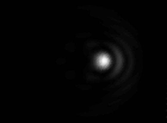
(a)

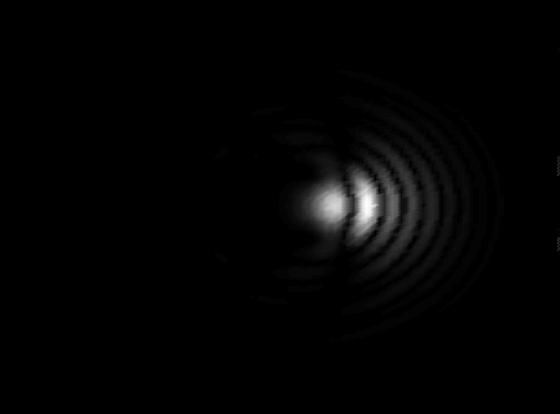
(b)

(c)

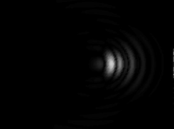
(d)

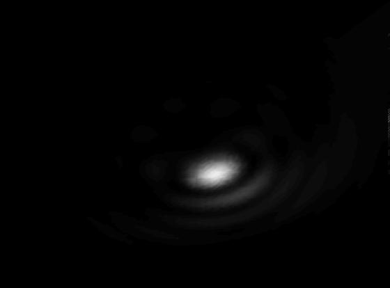
(e)

(f)

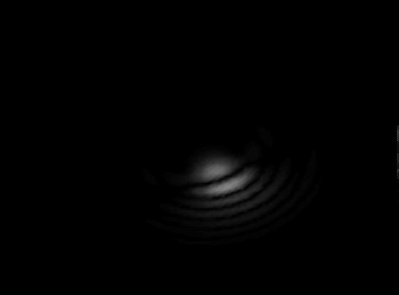
(g)

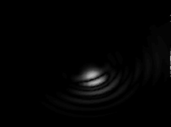
(h)

Figure 1: PSF for a helicity +1 source at (a) zero defocus and (e) defocus 8. The plots (b)-(d) display the magnitude of the difference between the PSF power when the source is in helicity -1, unpolarized, and $x$-polarized states, respectively, and the PSF power shown in (a) for the helicity +1 source, all for zero defocus. Plots (f)-(h) are the corresponding difference-magnitude plots for defocus 8. For the ease of visualization, the gray scale used for the difference plots is 1/6.8 times that used for the full PSF plots (a) and (e).

The 10-15% variation in the PSF (3D Source Localization and Polarimetry using High Numerical Aperture Imaging with Rotating PSF) with changing polarization seen in these figures should be sufficient to recover sensitively the polarization state of the source emission in an imager of sufficiently high NA, as we next confirm by computer simulation.

We simulated image data for a single point-dipole emitter operating under varying SNR conditions for the Gaussian additive-sensor-noise and Poisson photon-shot-noise models. Three different closely spaced values of the Stokes vector were selected for the simulation, all with $s_{0}=1$, $s_{1}=s_{2}=0$, but with $s_{3}$ taking values 0.8, 0.9, and 1. The first two values of $s_{3}$ correspond to the source polarization being in a mixed state in which a small incoherent admixture of the negative-helicity CP state corrupts the purity of the positive-helicity CP state, while the last value of $s_{3}$ represents the pure positive-helicity CP state. We formulate the inverse problem of reconstructing the Stokes vector from the noisy image data as a simple $\chi^{2}$-minimization problem with respect to the three free Stokes parameters, $s_{1}$, $s_{2}$, and $s_{3}$, with the value of $s_{0}$ fixed (here at 1) as the overall photon-flux normalization parameter. We employed the Matlab code fminunc to perform the minimization for each noisy image realization at each value of the peak SNR (PSNR), defined as the ratio of the peak image-pixel signal value, $I_{0}$, and the standard deviation of the noise at that pixel, the latter being equal to $I_{0}^{1/2}$ for the shot-noise case. The ratio $R/z_{I}$ was again chosen to be 1.

(a)

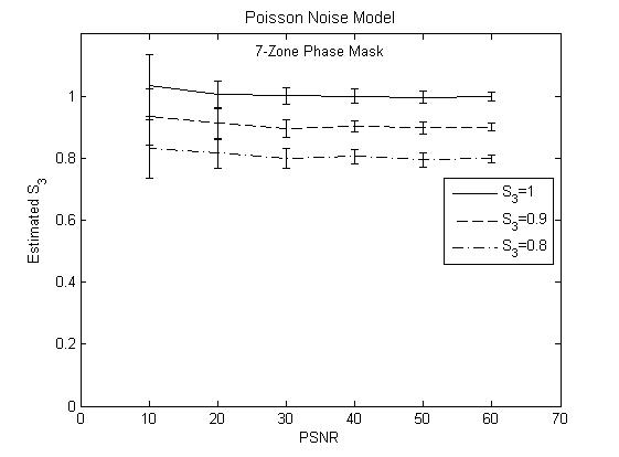
(b)

Figure 2: Reconstructed Stokes parameter $s_{3}$, shown with $\pm 1\sigma$ error bars, vs. PSNR for the (a) Gaussian additive sensor noise and (b) Poisson shot noise models.

From the plots of the reconstructed $s_{3}$, with $\pm 1\sigma$ error bars obtained from reconstructions from 30 different noise realizations for each PSNR value in each noise model, we see that at PSNR values exceeding 30, we can discriminate between closely spaced values of the $s_{3}$ parameter at the 10% level from the polarization-dependent PSFs of the kind shown in Fig. 1. The performance under the Poisson noise model is somewhat superior, with smaller error bars. For either noise model, higher statistical fidelity of discrimination than at the $\pm 1\sigma$ level would obviously require higher PSNR values. Although not shown here, similar error bars were obtained for other choices of the Stokes vector too, confirming its robust recovery by our polarimetric imager under fairly general conditions. Finally, we simulated image data for spiral phase masks with different total zone numbers and verified that, as expected, with a smaller (larger) number of zones in the mask, the relative contribution of the SAM-dependent wave polarization to PSF rotation is larger (smaller), thus lowering (raising) the PSNR threshold for a reliable estimation of the Stokes vector.

Unlike other polarimetric imagers GPY10 ; Sasagawa13 , our rotating-PSF-based polarimetric imager can sense both the 3D locations and polarization states of point sources in a single snapshot over a large focal volume without requiring specialized sensing elements. The performance of the proposed imager for multiple, closely spaced point sources in a 3D scene will be treated elsewhere.

The work was supported by the US Air Force Office of Scientific Research under grant no. F9550-11-1-0194.

References

- (1) S. Prasad, “Rotating point spread function via pupil-phase engineering,” Opt. Lett. 38, 585-587 (2013).
- (2) S. Pavani and R. Piestun, “High-efficiency rotating point spread functions,” Opt. Express 16, 3484-3489 (2008).
- (3) M. Lew, S. Lee, M. Badieirostami, and W. Moerner, “Corkscrew point spread function for far-field three-dimensional nanoscale localization of point objects, Opt. Lett. 36, 202-204 (2011).
- (4) G. Grover, K. DeLuca, S. Quirin, J. DeLuca, and R. Piestun, “Super-resolution photon-efficient imaging by nanometric double-helix point spread function localization of emitters (SPINDLE),” Opt. Express 20, 26681-26695 (2012).
- (5) M. Mansuripur, “Vector diffraction theory of focusing in high numerical aperture systems,” Opt. Photon. News, 73-75 (Mar 1992).
- (6) T. Jabbour and S. Kuebler, “Vector diffraction analysis of high numerical aperture focused beams modified by two- and three-zone annular multi-phase plates,” Opt. Express 14, 1033-1043 (2006).
- (7) Y. Tang, S. Hu,Y. Yang, and Y. He, “Focusing property of high numerical aperture photon sieves based on vector diffraction,” Opt. Commun. 295, 1-3 (2013).
- (8) J. Jackson, Classical Electrodynamics, 2nd edition (Wiley, 1999).
- (9) J. Goodman, Introduction to Fourier Optics, 2nd edition (McGraw Hill, 1996), Chap. 3.
- (10) V. Mahajan, Aberration Theory Made Simple (SPIE, 1991), Chap. 8.
- (11) A large NA is not entirely consistent with paraxial propagation assumed here, but is used here mainly to illustrate its importance for polarimetric imaging.
- (12) V. Gruev, R. Perkins, and T. York, “CCD polarization imaging sensor with aluminum nanowire optical filters,” Opt. Express 18, 19087-19094 (2010).
- (13) K. Sasagawa, S. Shishido, K. Ando, H. Matsuoka, T. Noda, T. Tokuda, K. Kakiuchi, and J. Ohta1,“Image sensor pixel with on-chip high extinction ratio polarizer based on 65-nm standard CMOS technology aluminum nanowire optical filters,” Opt. Express 21, 11132-11140 (2013).