Non-equilibrium dynamics of coupled Luttinger liquids

Abstract

In this work we consider the dynamics of two tunnel coupled chains after a quench in the tunneling strength is performed and the two systems are let evolve independently. We describe the form of the initial state comparing with previous results concerning the dynamics after the splitting of a one-dimensional gas of bosons into two phase coherent systems. We compute different correlation functions, among which those that are relevant for interference measurements, and discuss the emergence of effective temperatures also in connection with previous works.

I Introduction

The study of the non-equilibrium dynamics in closed quantum systems is a theoretical challenge that has been posed long time ago Neumann (1929); Deutsch (1991); Srednicki (1994); Polkovnikov et al. (2011) and it is now receiving enormous interest thanks to the possibility of exploring this regime in the laboratories, in particular in cold atomic experiments Bloch et al. (2008). These experiments allow one to access the intrinsic quantum many-body dynamics of the system without dissipation and in a controllable manner. Indeed, in this set up the system can be driven out-of-equilibrium by a sudden change of the interaction strength among the atoms or of the confining potential. Among others, one of the central questions in the field concerns the understanding of the relaxation of the system and the possibility to describe the final state as a thermal one with a well-defined effective temperature Polkovnikov et al. (2011); Cazalilla and Rigol (2010).

In this respect, thanks to their analytical tractability, one dimensional systems have been discussed quite extensively and have shown, in particular for integrable models, to lack equilibration to a Gibbs ensemble Kinoshita et al. (2006); Rigol et al. (2007); Calabrese et al. (2011); Caux and Konik (2012); Gurarie (2013). In many cases in fact correlation functions long after a quench in integrable models have been found compatible with a generalized Gibbs ensemble where many temperatures, one for each integral of motion, are introduced. Very recently generalized Gibbs ensembles have been observed experimentally Langen et al. (2014). Besides the characterization of the stationary regime, the relaxation of these systems has triggered lot of attention both theoretically Calabrese and Cardy (2006); Cheneau et al. (2012) and experimentally Cheneau et al. (2012); Langen et al. (2013) and it has been shown to occur via a light-cone dynamics that emerges thanks to the finite velocity of propagation of quasiparticles Calabrese and Cardy (2006); Cheneau et al. (2012); Langen et al. (2013).

Remarkable setups to explore these questions of out of equilibrium phyisics have been provided by atom-chips experiments Reichel and Vuletic (2010); Hofferberth et al. (2007); Gring et al. (2012); Langen et al. (2013, 2014) where one dimensional systems can be realized. In such experiments a one dimensional gas of bosons is split coherently into two systems by growing a potential barrier along the longitudinal axes Hofferberth et al. (2007); Gring et al. (2012); Langen et al. (2013).

Coupled with theoretical analysis Kitagawa et al. (2011); Smith et al. (2013); Gring et al. (2012); Langen et al. (2013) this study revealed that, depending on the splitting process, the dynamics proceeds via a prethermalized state, which shows certain equilibrium-like correlation functions despite being a non-equilibrium state. In particular, it was found that despite the integrability of the model under study, the system and its correlation functions are well described by thermal ones, with an effective temperature that is independent of the initial temperature of the system.

However, while the Hamiltonian dynamics after the splitting is well defined, more difficult is the description of the initial state as prepared in the process of splitting. In particular different splitting process give rise to correlation functions that are better described by a many temperature scenario Langen et al. (2014).

In this paper we examine a related model in which a similar analysis can be done in a controlled manner using Luttinger liquid theory. We look at the dynamics of two chains of bosonic particles that are equilibrated with a large finite coupling between the two chains and that are subsequently let evolve independently. This type of protocol can be performed with cold atoms, for instance in optical lattices where ladders have been realized Atala et al. (2014).

In particular in precedent works on the splitting of the gas Bistritzer and Altman (2007); Kitagawa et al. (2011); Gring et al. (2012) the initial state was taken as a Gaussian squeezed state. This form of the initial state was justified by the fact of recovering certain correlation functions at time $t=0$. In this work we give an alternative and more microscopic justification to the squeezed form and at the same time we discuss some differences found between the state that was used in Bistritzer and Altman (2007); Kitagawa et al. (2011); Gring et al. (2012) and the one that we derive in this work.

Moreover we also analyze the relaxation of the system from the time dependent to the stationary state and we discuss the possibility to define an effective temperature long after the quench, by inspecting several correlation functions.

The paper is organized as follows: in section II we introduce the model under study and the way it is analytically treated; in section III.1 we discuss the form of the initial state considered in previous works focussing on the splitting of the condensate, in section III.2 we describe the initial state that is recovered considering a quench of the tunneling term between the two chains and in section III.3 we discuss the comparison between the two forms; in section IV we discuss the occupation of the modes after the quench; in section V we derive the correlation functions which are relevant for interference experiments and in section VI we compute correlation functions associated to the density and the current. Finally in section VII we discuss our results and section VIII summarizes the work giving some perspectives.

II Interacting condensates: quadratic approximation

The system is prepared as two tunnel coupled one-dimensional chains. The Hamiltonian of the two systems at time $t=0$ is well described within the Luttinger liquid theory by Giamarchi (2003):

$$H^{1+2}=H_{LL}^{1}+H_{LL}^{2}-\,\frac{t_{\perp}}{2\pi}\,\int{\rm d}x\,2\cos(\theta_{2}(x)-\theta_{1}(x))\ .$$ (1)

Here $H_{LL}^{\alpha}$ is the Luttinger liquid Hamiltonian describing each chain $\alpha=1,2$:

$$H_{LL}^{\alpha}=\frac{\hbar u}{2}\int{\rm d}x\,\Big{[}\,\frac{\mathcal{K}}{\pi}\,[\nabla\theta_{\alpha}(x)]^{2}\,+\,\frac{\pi}{\mathcal{K}}[n_{\alpha}(x)]^{2}\,\Big{]}\ .$$ (2)

$\mathcal{K}$ is the Luttinger parameter and $u$ the sound velocity. The effects of interactions are hidden in those two parameters. In the weakly interacting regime the Luttinger parameter is $\mathcal{K}=\hbar\pi\sqrt{\frac{\rho}{mg}}$ in terms of the microscopic parameters of the gas, where $g$ is the effective interaction constant and $\rho$ the density. The hard core limit is instead achieved for $\mathcal{K}=1$. The sound velocity is given by $u=\hbar\pi\rho/m\mathcal{K}$ and therefore $u=\sqrt{\frac{\rho g}{m}}$ in the weakly interacting regime. The operators $\theta_{\alpha}(x)$ and $n_{\alpha}(x)$ representing respectively the phase of the bosonic field and the fluctuation of its density in the system $\alpha=1,2$ are canonically conjugated: $[n_{\alpha}(x),\theta_{\beta}(x^{\prime})]=i\delta(x-x^{\prime})\delta_{\alpha,\beta}$. The cosine term originates from the tunneling operator $\psi_{1}^{{\dagger}}(x)\psi_{2}(x)+\text{h.c.}=2\,\rho\cos(\theta_{2}(x)-\theta_{1}(x))$, where we used that $\psi_{\alpha}(x)\simeq\sqrt{\rho}\,e^{i\theta_{\alpha}(x)}$. Therefore one can set $t_{\perp}=\,\hbar\,J\rho$.

The dynamics of this system can be studied by introducing symmetric and antisymmetric variables $\theta_{A/S}=\theta_{1}\mp\theta_{2}$ and $n_{A/S}=(n_{1}\mp n_{2})/2$. Indeed under the assumption that the two systems are identical, symmetric and antisymmetric modes decouple and in terms of those variables one has $H=H_{LL}^{S}+H_{SG}^{A}$ with $H_{SG}^{A}$ the Sine-Gordon Hamiltonian for the antisymmetric modes:

$$\begin{array}[]{ll}\displaystyle H_{SG}^{A}=&\displaystyle\frac{\hbar u}{2}\,\int{\rm d}x\,\Big{[}\,\frac{K}{\pi}[\nabla\theta_{A}(x)]^{2}+\frac{\pi}{K}[n_{A}(x)]^{2}\,\Big{]}\\ \vspace{-0.2cm}\\ &\displaystyle\qquad-\,\frac{t_{\perp}}{2\pi}\,\int{\rm d}x\,2\,\cos\,\theta_{A}(x)\ ,\end{array}$$ (3)

where $K=\mathcal{K}/2$. In the following we will focus only on the antisymmetric part of $H$.

A limit which is particularly relevant for the next discussion is the case of $t_{\perp}=0$ when $H^{A}_{SG}$ reduces to the Luttinger liquid Hamiltonian which in its diagonal form reads:

$$H^{A}_{LL}=\sum_{p\neq 0}\hbar u|p|b^{{\dagger}}_{p}b_{p}+\frac{\hbar u\pi}{2K}n_{0}^{2}\ ,$$ (4)

made of non interacting sound wave modes. In order to obtain (4) we have expanded the fields $n_{A}(x)$ and $\theta_{A}(x)$ over the bosonic operators that diagonalize $H^{A}_{LL}$:

$$\begin{array}[]{ll}\displaystyle\theta_{A}(x)=&\displaystyle\frac{i}{\sqrt{L}}\sum_{p\neq 0}\ e^{-ipx}e^{-\alpha^{2}p^{2}/2}\sqrt{\frac{\pi}{2K|p|}}(b^{{\dagger}}_{p}-b_{-p})\\ \vspace{-0.2cm}\\ &\displaystyle\qquad+\,\frac{1}{\sqrt{L}}\theta_{0}\end{array}$$ (5)

$$\begin{array}[]{ll}\displaystyle n_{A}(x)=&\displaystyle\,\frac{1}{\sqrt{L}}\sum_{p\neq 0}e^{-ipx}e^{-\alpha^{2}p^{2}/2}\sqrt{\frac{|p|K}{2\pi}}(b^{{\dagger}}_{p}+b_{-p})\\ \vspace{-0.2cm}\\ &\displaystyle\qquad+\,\frac{1}{\sqrt{L}}n_{0}\ .\end{array}$$ (6)

where $\alpha$ is a cutoff regularizing the integrals.

We treat the cosine term in (3) for $t_{\perp}\neq 0$ by making a semiclassical expansion in $\theta_{A}$ around its minimum $\theta_{A}(x)=0$. This approximation greatly simplifies the problem, turning the Hamiltonian into a quadratic one. Indeed, under these conditions, the Hamiltonian reads (up to irrelevant constants):

$$\begin{array}[]{ll}\displaystyle H^{A}_{SC}&=\displaystyle\frac{u\hbar}{2}\int{\rm d}x\,\Big{[}\,\frac{K}{\pi}\,[\nabla\theta_{A}(x)]^{2}\,+\,\frac{\pi}{K}[n_{A}(x)]^{2}\,\Big{]}\\ \vspace{-0.2cm}\\ &\qquad\qquad\displaystyle+\frac{t_{\perp}}{2\pi}\int{\rm d}x(\theta_{A}(x))^{2}\ .\end{array}$$ (7)

Such semiclassical expansion is well adapted when $K$ is very large, as in the experiments Gring et al. (2012). In order to diagonalize the Hamiltonian $H^{A}_{SC}$ (7) for generic $t_{\perp}$ we note that under the quadratic approximation all $p$-modes are decoupled. The Hamiltonian (7) is made diagonal through the following transformation involving the bosonic modes with $p\neq 0$:

$$\begin{array}[]{ll}\displaystyle\eta_{p}^{{\dagger}}=\cosh\varphi_{p}b_{p}^{{\dagger}}-\sinh\varphi_{p}b_{-p}\\ \vspace{-0.2cm}\\ \displaystyle\eta_{-p}=\cosh\varphi_{p}b_{-p}-\sinh\varphi_{p}b_{p}^{{\dagger}}\ .\end{array}$$ (8)

The operators $\{\eta_{p},\eta^{{\dagger}}_{p}\}$ satisfy canonical bosonic commutation relations and $\varphi_{p}=\varphi_{-p}$ is fixed by the condition:

$$\tanh 2\varphi_{p}=\frac{t_{\perp}}{t_{\perp}+2K\hbar u|p|^{2}}\qquad\varphi_{p}=\frac{1}{2}\log\frac{\omega_{p}}{u|p|}\ ,$$ (9)

with $\omega_{p}=\sqrt{(\hbar up)^{2}+\frac{t_{\perp}\hbar u}{K}}=\sqrt{(\hbar up)^{2}+m^{2}}$, where we set $\displaystyle m^{2}\equiv\frac{\hbar ut_{\perp}}{K}$. The $p=0$ component of the Hamiltonian is made diagonal by the transformation:

$$\eta_{p=0}^{{\dagger}}=\frac{1}{\sqrt{2}}(\frac{n_{0}}{\sqrt{w}}-i\sqrt{w}\,\theta_{0})$$ (10)

with $w=\frac{mK}{\hbar u\pi}$. With these transformations the Hamiltonian becomes:

$$\begin{array}[]{ll}\displaystyle H^{A}_{SC}&\displaystyle=\sum_{p}\hbar\omega_{p}\eta_{p}^{{\dagger}}\eta_{p}\ .\end{array}$$ (11)

With respect to the Luttinger liquid Hamiltonian we see that the interaction $t_{\perp}$ in (11) opens a gap and turns the spectrum $\omega_{p}$ at small $p$ into a quadratic one.

III Initial state

III.1 Phenomenological derivation

As we mentioned in the introduction the theoretical framework of the previous section, and in particular the dynamics at $t_{\perp}=0$, is relevant to be compared with the description of experiments where a single gas is split into two gases which are let evolve independently. In the literature the initial state after the splitting of the system is taken of the following form Kitagawa et al. (2011); Gring et al. (2012):

$$|\tilde{\psi}_{0}\rangle=\frac{1}{\mathcal{N}}\exp\Big{[}\sum_{p>0}\tilde{W}_{p}b_{p}^{{\dagger}}b_{-p}^{{\dagger}}\Big{]}|0\rangle|\tilde{\psi}_{p=0}\rangle$$ (12)

and $\displaystyle\tilde{W}_{p}=\frac{1-\tilde{\alpha}_{p}}{1+\tilde{\alpha}_{p}}$, $\displaystyle\tilde{\alpha}_{p}=\frac{|p|K}{\pi\rho}$, $\langle n_{0}|\tilde{\psi}_{p=0}\rangle=e^{-\frac{1}{2\rho}n_{0}^{2}}$. Here $K$ is the Luttinger parameter and $\rho$ the density. $\mathcal{N}$ is the normalization of the state $\mathcal{N}=\prod_{p>0}(1-\tilde{W}_{p}^{2})^{-1/2}$. This form of the initial state is taken to reproduce the following correlation functions:

$$\begin{array}[]{ll}\displaystyle\langle n_{A}(p)n_{A}(p^{\prime})\rangle(t=0)=\frac{\rho}{2}\,\delta_{-p,p^{\prime}}\ ,\\ \vspace{-0.2cm}\\ \displaystyle\langle\theta_{A}(p)\theta_{A}(p^{\prime})\rangle(t=0)=\frac{1}{2\rho}\,\delta_{-p,p^{\prime}}\ ,\end{array}$$ (13)

resulting in local correlations in real space $\langle n_{A}(x)n_{A}(x^{\prime})\rangle(t=0)=\frac{\rho}{2}\,\delta(x-x^{\prime})$. These correlation functions should be considered with the delta function smeared over the healing length scale $\xi_{h}=\hbar u/g\rho$. This form of state is chosen assuming that the splitting leads to a random process where particles can go either left or right with equal probability. In the limit of large number of particles this process results in a Gaussian distribution of particle number difference where density fluctuations after the splitting are chosen to be proportional to the density itself. The strength of phase fluctuations follows considering the state as a minimum uncertainty state. In the following we will give a different explanation of how a state of the form (12) should be expected. The analogous coefficient $\tilde{W}_{p}$ will be slightly different.

III.2 Quench in $t_{\perp}$

In this section we take as initial state the one resulting from a sudden quench of $t_{\perp}$. This means that we assume that the initial state is prepared equilibrating the system in the ground state of the Hamiltonian (7) at large $t_{\perp}$ and then suddenly change $t_{\perp}$ of a finite amount. In particular we will compare this result with the one of the previous section in the case where the dynamics is driven with $t_{\perp}=0$. Hereafter we will set $\hbar=1$. A similar situation concerning a quench of the mass in a bosonic field theory was considered in Sotiriadis and Cardy (2010); Sotiriadis et al. (2013); Iucci and Cazalilla (2010).

The Hamiltonian at time $t=0$ is associated with a bosonic operator $\eta_{p}^{0}$ such that the initial state is the vacuum of this operator $\eta_{p}^{0}|\psi_{0}\rangle=0$.

One can show that in terms of the bosonic operators $b_{p}^{{\dagger}}$, $b_{p}$ diagonalizing the Hamiltonian (7) with $t_{\perp}=0$ the initial state has a squeezed form of the type (12):

$$|\psi_{0}\rangle=\frac{1}{\mathcal{N}}\exp\Big{[}\sum_{p>0}W_{p}b_{p}^{{\dagger}}b_{-p}^{{\dagger}}\Big{]}|0\rangle|\psi_{p=0}\rangle\ ,$$ (14)

where the coefficients $W_{p}$ are now different from (12).

Indeed, one can compute the action of the operator $\eta_{p}^{0}$ over a state with a squeezed form as in (14), after performing a Bogoliubov transformation as in (8). Taking $|\psi_{0}\rangle$ as in (14) and considering $p\neq 0$ one obtains:

$$\begin{array}[]{ll}\displaystyle\eta_{p}^{0}|\psi_{0}\rangle&\displaystyle=\Big{(}\cosh\varphi_{p}^{0}b_{p}-\sinh\varphi_{p}^{0}b_{-p}^{{\dagger}}\Big{)}|\psi_{0}\rangle\\ \vspace{-0.2cm}\\ &\displaystyle=\cosh\varphi_{p}^{0}W_{p}b_{-p}^{{\dagger}}|\psi_{0}\rangle-\sinh\varphi_{p}^{0}b_{-p}^{{\dagger}}|\psi_{0}\rangle\ .\end{array}$$ (15)

Imposing $\displaystyle\eta_{p}^{0}|\psi_{0}\rangle=0$ one finds $W_{p}=\text{tanh}\,\varphi_{p}^{0}=\frac{1-\alpha_{p}}{1+\alpha_{p}}=\frac{1-\frac{u|p|}{\omega_{p}^{0}}}{1+\frac{u|p|}{\omega_{p}^{0}}}$. This form of squeezed state was also found in Sotiriadis et al. (2013). The component $p=0$ can be written as $|\psi_{p=0}\rangle\propto e^{-\frac{n_{0}^{2}}{2w}}|0\rangle$ with $\theta_{0}|0\rangle=0$. In fact

$$\eta_{p=0}^{0}|\psi_{p=0}\rangle=\frac{1}{\sqrt{2}}(\frac{n_{0}}{\sqrt{w}}+i\sqrt{w}\,\theta_{0})|\psi_{p=0}\rangle=0$$ (16)

where we used $[\theta_{0},n_{0}]=-i$ and $[\theta_{0},f(n_{0})]=[\theta_{0},n_{0}]f^{\prime}(n_{0})$.

III.3 Comparison of the two forms

Let us now compare the results of the phenomenological derivation (12) with our ladder case (14). Considering the values given after (12) one has to compare $\alpha_{p}=\frac{u|p|}{\omega_{p}^{0}}$ with $\tilde{\alpha}_{p}=\frac{|p|K}{\pi\rho}$.

The two expressions present points of similarity and of difference. Indeed, to go from one to the other one has to change $\omega_{p}^{0}\to\frac{\pi\rho u}{K}$. In the limit of non-zero tunneling (which is the case for our initial state) and small momenta one can approximate $\omega_{p}^{0}\simeq m^{0}=\sqrt{\frac{J_{0}\rho u}{K}}$

This calculation shows that a quench in $t_{\perp}$ would lead to a state with a squeezed form in $b_{p}^{{\dagger}}b_{-p}^{{\dagger}}$ and the coefficients that agree with the one used in (12) in the limit of small momenta for what concerns the dependence in $p$ but not in the coefficient of proportionality.

IV Effective temperature

It has been shown that the state (12) leads to correlation functions that are well described by an effective temperature $T_{\rm eff}=\frac{\pi u\rho}{4K}$ Smith et al. (2013); Gring et al. (2012).

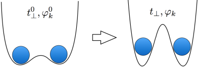
Figure 1: Schematic figure representing the quench from high to low tunnel-coupled systems. The two states are characterized respectively by a given tunneling strength $t_{\perp}^{0}$ and $t_{\perp}$ and Bogolioubov angles $\varphi^{0}_{k}$ and $\varphi_{k}$.

In order to see the differences in the effective temperature that emerges between $|\tilde{\psi}_{0}\rangle$ in (12) and $|\psi_{0}\rangle$ in (14) we now consider a quench from the squeezed state characterized by $\varphi_{p}^{0}$ towards a situation where the barrier is higher and the bosonic operator are associated with an angle $\varphi_{p}$ (see Fig, 1). The case of independent systems and thus of infinite barrier corresponds to $\varphi_{p}=0$. The mapping between the operators diagonalizing the pre and post quench Hamiltonian reads as follows:

$$\begin{array}[]{ll}\displaystyle\eta_{p}&\displaystyle=\cosh\Big{(}\varphi_{p}-\varphi_{p}^{0}\Big{)}\,\eta_{p}^{0}-\sinh\Big{(}\varphi_{p}-\varphi_{p}^{0}\Big{)}\,\eta_{-p}^{0{\dagger}}\end{array}$$ (17)

We note that:

$$\frac{\Delta_{p}}{2}=\varphi_{p}-\varphi_{p}^{0}=\frac{1}{2}\log\frac{\omega_{p}}{\omega_{p}^{0}}$$ (18)

and the occupation of the modes reads:

$$\begin{array}[]{ll}\displaystyle\text{cotanh}\frac{\beta_{\rm eff}(p)\omega_{p}}{2}&\displaystyle=2\langle\eta_{p}^{{\dagger}}\eta_{p}\rangle+1=\frac{1}{2}\Big{(}\frac{\omega_{p}}{\omega_{p}^{0}}\,+\frac{\omega_{p}^{0}}{\omega_{p}}\,\Big{)}\\ \vspace{-0.2cm}\\ &\displaystyle=\cosh\Delta_{p}\ ,\end{array}$$ (19)

which is the analogue of the formulas derived within other quenches and quadratic models Calabrese et al. (2011); Foini et al. (2011). This leads to $p$-dependent effective temperatures:

$$\beta_{\rm eff}(p)=\frac{1}{\omega_{p}}\,\log\,\frac{\cosh\Delta_{p}+1}{\cosh\Delta_{p}-1}=\frac{2}{\omega_{p}}\,\log\,\frac{\omega_{p}+\omega_{p}^{0}}{|\omega_{p}-\omega_{p}^{0}|}$$ (20)

as found in Sotiriadis et al. (2009). If one takes the limit of small momenta and assume that $m^{0}\gg m$ this formula gives $T_{\rm eff}=\frac{m^{0}}{4}=\frac{1}{4}\sqrt{\frac{J_{0}u\rho}{K}}$. One should therefore compare this temperature with the one found in Kitagawa et al. (2011); Gring et al. (2012) which is $\tilde{T}_{\rm eff}=\frac{\pi u\rho}{4K}$. Clearly, the two formulas show different dependences on the density, the sound velocity and the Luttinger parameter.

V Dynamics of the phase

In the following we focus on the dynamics after the quench of $t_{\perp}$ and consider correlation functions that are relevant for interference experiments. We define $n_{p}=\sqrt{\frac{|p|K}{2\pi}}(b^{{\dagger}}_{p}+b_{-p})$ and $\theta_{p}=i\sqrt{\frac{\pi}{2K|p|}}(b^{{\dagger}}_{p}-b_{-p})$. Under the quench protocol described in the previous section correlation functions at time $t=0$ have the following form:

$$\begin{array}[]{ll}\displaystyle\langle\psi_{0}|n_{p}n_{p^{\prime}}|\psi_{0}\rangle(t=0)=\delta_{p^{\prime},-p}\frac{K}{2\pi u}\omega_{p}^{0}\\ \vspace{-0.2cm}\\ \displaystyle\ \langle\psi_{0}|\theta_{p}\theta_{p^{\prime}}|\psi_{0}\rangle(t=0)=\delta_{p^{\prime},-p}\frac{\pi u}{2K}\frac{1}{\omega^{0}_{p}}\ .\end{array}$$ (21)

We consider the dynamics of the system when $t_{\perp}=0$ and the two condensates evolve independently.

From the interference one is able to extract the following correlation functions Polkovnikov et al. (2006); Gring et al. (2012); Langen et al. (2013):

$$C_{\theta}(x,t)=\frac{\langle\psi_{1}(x)\psi^{{\dagger}}_{2}(x)\psi^{{\dagger}}_{1}(0)\psi_{2}(0)\rangle}{\langle|\psi_{1}(x)|^{2}\rangle\langle|\psi_{2}(x)|^{2}\rangle}$$ (22)

which involves the relative phase between the two condensate and reads:

$$C_{\theta}(x,t)=\langle e^{i[\theta_{A}(x,t)-\theta_{A}(0,t)]}\rangle=e^{-\frac{1}{2}\langle[\theta_{A}(x,t)-\theta_{A}(0,t)]^{2}\rangle}$$ (23)

where:

$$\begin{array}[]{ll}\displaystyle\langle[\theta_{A}(x,t)-\theta_{A}(0,t)]^{2}\rangle\displaystyle=\frac{1}{\pi}\int{\rm d}p\,(1-\cos px)e^{-\alpha^{2}p^{2}}\times\\ \vspace{-0.2cm}\\ \displaystyle\times\Big{[}\sin^{2}(u|p|t)\,\frac{\pi^{2}}{K^{2}p^{2}}\,\langle|n_{p}|^{2}\rangle(0)+\,\cos^{2}(u|p|t)\,\langle|\theta_{p}|^{2}\rangle(0)\Big{]}\ ,\end{array}$$ (24)

and $\alpha$ is a small cutoff regularizing the integral. In the upper panel of Fig. 2 we show the correlation function (23) as a function of space for four different times and the stationary limit. The lower panel shows the same correlation function as a function of time for three different space differences.

The stationary limit of this correlation function reads:

$$\begin{array}[]{ll}\displaystyle\lim_{t\to\infty}\langle[\theta_{A}(x,t)-\theta_{A}(0,t)]^{2}\rangle&\displaystyle=\frac{1}{2\pi K}\int{\rm d}p\,(1-\cos px)e^{-\alpha^{2}p^{2}}\Big{[}\,\frac{\pi}{p^{2}}\,\frac{1}{2u}\sqrt{m_{0}^{2}+(up)^{2}}+\,\frac{\pi u}{2}\frac{1}{\sqrt{m_{0}^{2}+(up)^{2}}}\Big{]}\\ \vspace{-0.2cm}\\ &\displaystyle=\frac{1}{K}\int_{0}^{\infty}{\rm d}p\,(1-\cos px)e^{-\alpha^{2}p^{2}}\frac{1}{p}\cosh\Delta_{p}\ ,\end{array}$$ (25)

and it turns out to be different from the thermal equilibrium correlation function. Yet if $m_{0}\alpha/u\gg 1$ one can expand and obtain:

$$\begin{array}[]{ll}\displaystyle\lim_{t\to\infty}\langle[\theta_{A}(x,t)-\theta_{A}(0,t)]^{2}\rangle\displaystyle\simeq\frac{1}{K}\int_{0}^{\infty}{\rm d}p\,(1-\cos px)\times\\ \vspace{-0.2cm}\\ \displaystyle\qquad\qquad\qquad\times e^{-\alpha^{2}p^{2}}\,\frac{m_{0}}{2up^{2}}\stackrel{{\scriptstyle xm_{0}/u\gg 1}}{{\simeq}}\frac{\pi m_{0}x}{4uK}\ .\end{array}$$ (26)

This asymptotic form should be compared with the equilibrium:

$$\begin{array}[]{ll}\displaystyle\langle[\theta_{A}(x)-\theta_{A}(0)]^{2}\rangle_{T_{\rm eff}}=\displaystyle\frac{1}{K}\int_{0}^{\infty}{\rm d}p\,(1-\cos px)e^{-\alpha^{2}p^{2}}\times\\ \vspace{-0.2cm}\\ \qquad\qquad\qquad\displaystyle\times\frac{1}{p}\text{cotanh}\Big{(}\frac{u|p|}{2T_{\rm eff}}\Big{)}\\ \vspace{-0.2cm}\\ \qquad\qquad\displaystyle\simeq\displaystyle\frac{1}{K}\int_{0}^{\infty}{\rm d}p\,(1-\cos px)e^{-\alpha^{2}p^{2}}\frac{2T_{\rm eff}}{up^{2}}\end{array}$$ (27)

recovering $T_{\rm eff}=\frac{m_{0}}{4}$. In the upper panel of Fig. 3 we show the asymptotic correlation function $C_{\theta}(x,t\to\infty)=\exp(-\frac{1}{2}\lim_{t\to\infty}\langle[\theta_{A}(x,t)-\theta_{A}(0,t)]^{2}\rangle)$ as given in (25) with a black line and the thermal one with $T_{\rm eff}=\frac{m_{0}}{4}$ in blue. The two lines overlap remarkably and look indistinguishable.

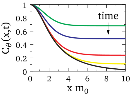
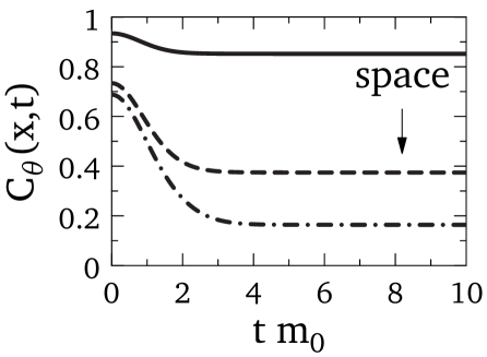
Figure 2: Correlation functions $C_{\theta}(x,t)$ (23), for different time and length scales. Here $K=1$, $u=1$ and $\alpha m_{0}=1$. Upper panel: $C_{\theta}(x,t)$ as a function of the space distance for four different times $tm_{0}=0.1,1,2,3$ shown respectively with green, blue, red and yellow lines. The black envelope is the asymptotic stationary correlation function. Lower panel: $C_{\theta}(x,t)$ as a function of the time, for three different space distances $xm_{0}=1,3,5$ shown respectively with solid, dashed and dotted-dashed lines.

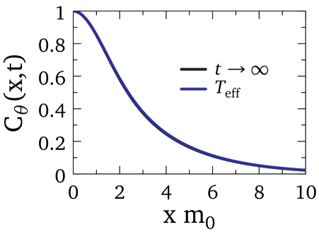
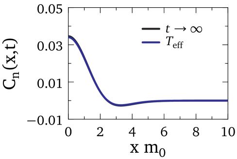
Figure 3: Upper panel: asymptotic correlation functions $C_{\theta}(x,t\to\infty)=\exp(-\frac{1}{2}\lim_{t\to\infty}\langle[\theta_{A}(x,t)-\theta_{A}(0,t)]^{2}\rangle)$ with $\lim_{t\to\infty}\langle[\theta_{A}(x,t)-\theta_{A}(0,t)]^{2}\rangle$ given in  (25) and thermal correlation function $C_{\theta}(x)=\exp(-\frac{1}{2}\langle[\theta_{A}(x)-\theta_{A}(0)]^{2}\rangle_{T_{\rm eff}})$ with $\langle[\theta_{A}(x)-\theta_{A}(0)]^{2}\rangle_{T_{\rm eff}}$ given in (27) shown with black and blue lines respectively. Lower panel: asymptotic correlation function of the relative density (29) (black line) compared with the equilibrium one (30) (blue line). In both plots $\alpha m_{0}=1$, $K=1$, $u=1$ and $T_{\rm eff}=\frac{m_{0}}{4}$.

VI Dynamics of the density and current

In this section we consider the dynamics of the relative density and current. The density can be experimentally recovered by taking images of the two systems. We consider again the dynamics at $t_{\perp}=0$ which results in the following correlation function:

$$\begin{array}[]{ll}\displaystyle C_{n}(x,t)=\langle n_{A}(x,t)n_{A}(0,t)\rangle=\frac{K}{4\pi^{2}}\int\ {\rm d}p\ e^{ipx}\ e^{-\alpha^{2}p^{2}}\times\\ \vspace{-0.2cm}\\ \qquad\qquad\displaystyle\times\Big{[}\sin^{2}\omega_{p}t\,\frac{p^{2}u}{\omega_{p}^{0}}+\,\cos^{2}\omega_{p}t\,\frac{\omega_{p}^{0}}{u}\Big{]}\ .\end{array}$$ (28)

The stationary value of this correlation function turns out to be:

$$\begin{array}[]{ll}\displaystyle C_{n}(x,t\to\infty)=\frac{K}{4\pi^{2}}\int\ {\rm d}p\ e^{ipx}\ e^{-\alpha^{2}p^{2}}\,\frac{1}{2}\,\Big{[}\frac{p^{2}u}{\omega_{p}^{0}}+\frac{\omega_{p}^{0}}{u}\Big{]}\\ \vspace{-0.2cm}\\ \qquad\qquad\displaystyle=\frac{K}{4\pi^{2}}\int\ {\rm d}p\ e^{ipx}\ e^{-\alpha^{2}p^{2}}\,|p|\cosh\Delta_{p}\ .\end{array}$$ (29)

In the upper panel of Fig. 4 we show the correlation function $C_{n}(x,t)$, as a function of the space distance for different times together with the asymptotic stationary result. From the plot one sees that for sufficiently large times (e.g. $tm_{0}=2,3,6$) the dynamical curves follow the stationary limit up to a distance that grows with time and then departs from it.

The equilibrium correlation function is given by:

$$\begin{array}[]{ll}\displaystyle\langle n_{A}(x)n_{A}(0)\rangle_{T_{\rm eff}}=&\displaystyle\frac{K}{4\pi^{2}}\int\ {\rm d}p\ e^{ipx}\ e^{-\alpha^{2}p^{2}}|p|\times\\ \vspace{-0.2cm}\\ &\displaystyle\qquad\quad\times\text{cotanh}\left(\frac{\omega_{p}}{2T_{\rm eff}}\right)\ .\end{array}$$ (30)

In the lower panel of Fig. 3 we show the asymptotic correlation function for the relative density (29) with a black line and the same correlation function at thermal equilibrium (30) at $T_{\rm eff}=\frac{m_{0}}{4}$ with a blue line. Also in this case the two functions are not the same but numerically they look indistinguishable showing that for all practical purposes this state can be considered as a thermal “equilibrium” state.

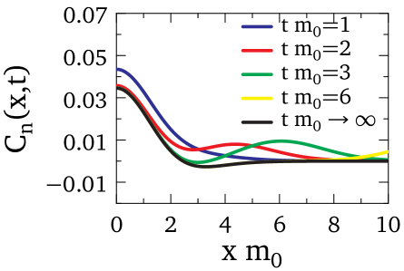
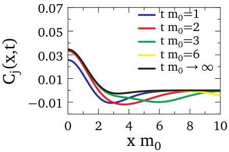
Figure 4: Correlation functions of the density $C_{n}(x,t)$ (upper panel) and of the current $C_{j}(x,t)$ (lower panel) as a function of the space distance for different times. Times $tm_{0}=1,2,3,6$ are shown respectively with blue, red, green and yellow lines. In both plots the black line is the asymptotic result in the stationary limit. In both figures we set $\alpha m_{0}=1$, $K=1$ and $u=1$. For the parameters used here the stationary curves in the two plots are the same.

It is natural to compare the correlation functions of the density with the ones involving the current $j_{A}(x)=-\frac{1}{\pi}\nabla\theta_{A}(x)$. The corresponding correlation function reads:

$$\begin{array}[]{ll}\displaystyle\displaystyle C_{j}(x,t)=&\displaystyle\langle j_{A}(x)j_{A}(0)\rangle=\displaystyle\frac{1}{4\pi^{2}K}\int\ {\rm d}p\ e^{ipx}\ e^{-\alpha^{2}p^{2}}\times\\ \vspace{-0.2cm}\\ &\displaystyle\qquad\times\Big{[}\sin^{2}\omega_{p}t\,\frac{\omega_{p}^{0}}{u}+\,\cos^{2}\omega_{p}t\,\frac{u\,p^{2}}{\omega_{p}^{0}}\Big{]}\par\end{array}$$ (31)

The stationary limit of (31) is the same as (29) with the substitution $K\to K^{-1}$. The same substitution gives the equilibrium correlation function associated to the current from (30). In the lower panel of Fig. 4 we show the correlation functions $C_{j}(x,t)$ as a function of the space for different times, in particular $tm_{0}=1,2,3,6$ are shown respectively with blue, red, green and yellow lines. The black line is the asymptotic result in the stationary limit.

VII Discussions

Let us now discuss some aspects of the results obtained in the previous sections and the model we have used to obtain them.

First we note that our results were obtained in the approximations of a quadratic expansion of the cosine term that encodes the interaction between the two condensates around the minimum $\theta_{A}=0$. Such an approximation is expected to work better in the weakly interacting regime (which is the one realized in Hofferberth et al. (2007); Gring et al. (2012); Langen et al. (2013)) where the cosine term is very relevant.

Under these assumptions we have shown that the form of the initial state is that of a squeezed state in terms of the operators that diagonalize the final Hamiltonian at $t_{\perp}=0$. This form is qualitatively the same as the one derived in Bistritzer and Altman (2007); Kitagawa et al. (2011); Gring et al. (2012) in order to describe the state obtained from the splitting of a one dimensional gas into two phase-coherent systems Hofferberth et al. (2007); Gring et al. (2012); Langen et al. (2013). The coefficients appearing in the squeezed form are nonetheless different and give raise to some differences in the physical quantities, as explained below.

Besides the characterization of the initial state, we have computed the correlation functions of the relative phase between the two systems, correlations that are relevant for interference experiments. From Fig. 2 one sees that these correlations initially show long range order at large distances, implying high interference contrast, and the value attained at large distances decays with time. In comparison with the correlation functions computed in Langen et al. (2013) the qualitative form is similar with the appearance of a light cone that separates the length scales into a region of short distances growing with time where the correlation functions have relaxed and a region of larger distances that keeps track of the initial correlation. This light cone scenario has been observed also in other works Calabrese and Cardy (2006); Iglói and Rieger (2011); Calabrese et al. (2011); Cheneau et al. (2012) and it is justified with the creation at time $t=0$ of elementary excitations that propagate in opposite direction and with finite velocity. In the case of $t_{\perp}=0$ the spectrum is linear and all quasi-particles move coherently with the same group velocity and two points at a given distance will equilibrate only when such quasi-particles have the time to travel along that length scale.

In addition to the correlation functions associated to the relative phase we have computed the evolution of the correlation functions describing the relative density and current (see Fig. 4, upper and lower panel respectively). These correlation functions do not show a clear light cone dynamics as for the relative phase, however, in a similar way, at large times the dynamical curves stay close to the asymptotic stationary line up to distances that grow with time.

For all phase, density and current correlation functions we have considered the limit of long times when they all become stationary. In this limit the analytical form of correlation functions is not compatible with that at thermal equilibrium, which is not surprising in view of the integrability of the dynamics and the Gaussian form of the initial state here considered. Nonetheless, numerically, stationary and thermal correlation functions are in remarkable agreement, so that experimentally one should not be able to distinguish between the two. The thermal correlation functions that we have considered are associated with an effective temperature $T_{\rm eff}=\frac{m_{0}}{4}=\frac{1}{4}\sqrt{\frac{J_{0}\rho u}{K}}$, where $m_{0}$ is the gap characterizing the spectrum before the quench, $J_{0}$ is the amplitude of the initial tunneling, $\rho$ the density, $u$ the speed of sound and $K$ le Luttinger parameter.

The agreement between the curves obtained as the stationary limit of the non-equilibrium process and the ones drawn with the effective temperature $T_{\rm eff}=\frac{m_{0}}{4}$ can be justified if one develops the asymptotic form of correlation functions at large $\frac{m_{0}\alpha}{u}$, where $\alpha$ is the cut-off, and develops the equilibrium correlation functions at large temperatures. However numerically one sees that the agreement is good also at small values of $\frac{m_{0}\alpha}{u}$.

Moreover we note that that if one assigns a different temperature to each mode by requiring the conservation of their occupation numbers, as in (20), the temperature $T_{\rm eff}=\frac{m_{0}}{4}$ is the one associated with the low energy modes.

Such an effective temperature, obtained within our quench protocol, should be contrasted with the one that it is found with the initial state describing the splitting process $\tilde{T}_{\rm eff}=\frac{\pi u\rho}{4K}$ Gring et al. (2012). The two expressions clearly indicate a different dependence in the density. In particular, in the weakly interacting regime where $\frac{u}{K}$ is independent of the density, the two procedures give raise respectively to a temperature that goes with $T_{\rm eff}\propto\sqrt{\rho}$ and one that is linear in the density $\tilde{T}_{\rm eff}\propto\rho$.

As we mentioned in the introduction, this quench protocol can be implemented experimentally, as ladders have already been realized Atala et al. (2014). The same theoretical description can be applied to describe atom-chip experiments, once two one dimensional gases are equilibrated with a finite barrier which is subsequently increased in order to suppress the tunneling between the two. In both cases the effective temperature could be extracted from the decay of the correlation functions sufficiently long after the quench.

It would be therefore interesting to compare the results obtained for the effective temperature in the splitting process with the ones of the quench that we propose.

VIII Conclusions

In this work we have considered two chains that are tunnel coupled through an interaction parameter $t_{\perp}$ which, at time $t=0$, is suddenly set to zero. We have shown that the form of the state after the quench is that of a squeezed state, similar (but not equal) to what was assumed in Kitagawa et al. (2011); Gring et al. (2012) from phenomenological arguments.

We have computed the correlation functions of the relative phase which are directly probed in interference experiments and the correlation functions of the relative density and current. For all of them we have extracted their asymptotic form as obtained at large times. We have shown that the stationary correlations are formally not compatible with the ones derived at thermal equilibrium. Nonetheless numerically all correlation functions in the stationary state and those at thermal equilibrium are in striking agreement. The effective temperature with which these correlation functions are compared is quite different from the one derived in Kitagawa et al. (2011); Gring et al. (2012); Langen et al. (2013). In our quench it is associated with the mass of the initial Hamiltonian and depends on the squared root of the density while the effective temperature found in  Kitagawa et al. (2011); Gring et al. (2012); Langen et al. (2013) is linear in the density.

In view of this difference it would be interesting to compare the effective temperature that is found after the splitting of the condensate with the one that one recovers considering the quench suggested in this work.

As a future work, it would be interesting to study the effect of the initial temperature on the subsequent dynamics, by considering as initial state a density matrix instead of the ground state of the Hamiltonian for some $t_{\perp}$. In fact, in Kitagawa et al. (2011); Gring et al. (2012); Langen et al. (2013) it was found that the effective temperature is insensitive to the temperature of the system before the splitting and it would be worth investigating up to which extent this property carries over in our quench protocol.