A Cycle-Based Formulation and Valid Inequalities for DC Power Transmission Problems with Switching

Abstract

It is well-known that optimizing network topology by switching on and off transmission lines improves the efficiency of power delivery in electrical networks. In fact, the USA Energy Policy Act of 2005 (Section 1223) states that the U.S. should “encourage, as appropriate, the deployment of advanced transmission technologies” including “optimized transmission line configurations.” As such, many authors have studied the problem of determining an optimal set of transmission lines to switch off to minimize the cost of meeting a given power demand under the direct current (DC) model of power flow. This problem is known in the literature as the Direct-Current Optimal Transmission Switching Problem (DC-OTS). Most research on DC-OTS has focused on heuristic algorithms for generating quality solutions or on the application of DC-OTS to crucial operational and strategic problems such as contingency correction, real-time dispatch, and transmission expansion. The mathematical theory of the DC-OTS problem is less well-developed. In this work, we formally establish that DC-OTS is NP-Hard, even if the power network is a series-parallel graph with at most one load/demand pair. Inspired by Kirchoff’s Voltage Law, we give a cycle-based formulation for DC-OTS, and we use the new formulation to build a cycle-induced relaxation. We characterize the convex hull of the cycle-induced relaxation, and the characterization provides strong valid inequalities that can be used in a cutting-plane approach to solve the DC-OTS. We give details of a practical implementation, and we show promising computational results on standard benchmark instances.

1 Introduction

An electric power grid is a complex engineered system whose control and operation is driven by fundamental laws of physics. The optimal power flow (OPF) problem is to determine a minimum cost delivery of a given demand for power subject to the power flow constraints implied by the network. The standard mathematical model of power flow uses alternating current (AC) power flow equations. The AC power flow equations are nonlinear and nonconvex, which has prompted the development of a linear approximation known as the direct current (DC) power flow equations. DC power flow equations are widely used in the current industry practice, and the DC OPF problem is a building block of power systems operations planning.

One consequence of the underlying physical laws of electric power flow is a type of “Braess’ Paradox” where removing lines from a transmission network may result in improved network efficiency. O’Neill et al. (2005) propose exploiting this well-known attribute of power transmission networks by switching off lines in order to reduce generation costs. Fisher et al. (2008) formalized this notion into a mathematical optimization problem known as the Optimal Transmission Switching (OTS) problem. The OTS problem is the OPF problem augmented with the additional flexibility of changing the network topology by removing transmission lines. While motivated in O’Neill et al. (2005) by an operational problem in which lines may be switched off to improve efficiency, the same mathematical switching structure appears also in longer-term transmission network expansion planning problems.

Because of the mathematical complexity induced by the AC power flow equations, nearly all studies to date on the OTS problem have used the DC approximation to power flow (e.g. see Fisher et al. (2008), Barrows et al. (2012), Fuller et al. (2012), Wu and Cheung (2013)). With this approximation, a mixed-integer linear programming (MILP) model for DC-OTS can be created and input to existing MILP software. In the MILP model, binary variables are used to model the changing topology and enforce the network power flow constraints on a line if and only if the line is present. Models with many “indicator constraints” of this form are often intractable for modern computational integer programming software, since the linear relaxations of the formulations are typically very weak. Previous authors have found this to be true for DC-OTS, and many heuristic methods have been developed based on ranking lines (Barrows et al. (2012), Fuller et al. (2012), Wu and Cheung (2013)), or by imposing an (artificial) cardinality constraint on the number of lines that may be switched off in a solution (Fisher et al. (2008)). The solutions found from these heuristics have demonstrated that significant efficiency gains are possible via transmission switching.

The paper by Coffrin et al. (2014) offers a criticism of the use of the DC-approximation to model power flow for the OTS problem. The paper demonstrates that a direct application of the DC power flow equations may not be accurate enough to recover useful AC operation solutions in the context of the OTS. They thus argue for the use of the AC-power flow equations in the OTS problem. The authors employ a convex quadratic relaxation of the AC power flow equations proposed in Hijazi et al. (2013) and embed the relaxation in a branch-and-bound method to solve the AC-OTS problem. The recent papers by Barrows et al. (2014) and Soroush and Fuller (2014) also develop methods and heuristics for AC-OTS.

Despite the criticism of the DC power flow model for optimal transmission switching, there are many planning problems where the DC power flow model may be an acceptable approximation when combined with network topology changes. A survey in Hedman et al. (2011) enumerates applications of transmission switching to improve voltage profiles, reduce congestion and losses in the system, and to increase reliability of the power grid. A standard reliability criterion for the power grid is that the system must be able to withstand an “$N-1$” event—in an interconnection network with $N$ elements, the system will operate reliably following the failure of any one of them. Hedman et al. (2009) augment the DC-OTS model to ensure that the $N-1$ reliability criteria is satisfied. Heuristics are used to iteratively decide which lines to be switched off, while preserving $N-1$ reliability for standard test cases. The authors show that significant cost savings from transmission switching is still possible even if the $N-1$ contingency is required.

Transmission switching is also an important subproblem in power grid capacity expansion planning. In Khodaei et al. (2010), a large MILP model is constructed to solve an expansion planning problem with contingencies, the DC power flow equations are used, and transmission switching is allowed in finding the best configuration. Villumsen and Philpott (2012) develop a slightly different model for expansion planning that also relies on the DC-power flow approximation and transmission switching. They employ their method on a case study for a real power system expansion plan in Denmark (see Villumsen et al. (2013)). In the context of expansion planning, it is important to note that the mathematical structure of line addition is exactly the same as line removal.

Authors who have combined the DC-approximation to power flow with the flexibility of modifying the network topology have found that the resulting MILP programming model is very challenging and called for a more systematic study on its underlying mathematical structure. For example, the authors of Hedman et al. (2010) state that

“When solving the transmission switching problem, $\ldots$ the techniques for closing the optimality gap, specifically improving the lower bound, are largely ineffective.”

A primary focus of our work is an attempt to change this reality by developing strong classes of valid inequalities that may be applied to power systems planning problems that involve the addition or removal of transmission elements. Our paper makes the following contributions:

• Using a formulation based on Kirchoff’s Voltage Law, we give a cycle-based linear mixed integer programming (MIP) formulation for DC-OTS.

• We formally establish that the DC-OTS problem is NP-Hard, even if the interconnection network is a series-parallel graph and there is only one generation/demand pair. (Additional complexity results were recently independently established by Lehmann et al. (2014)).

• Using the cycle-based formulation as inspiration, we derive classes of strong valid inequalities for a cycle–relaxation of the DC-OTS. We additionally establish that inequalities define the convex hull of the cycle-relaxation, and we show how to separate the inequalities over a given cycle in polynomial time.

• We perform computational experiments focusing on improving performance of integer programming-based methods for the OTS using the DC power flow approximation. We show that the new inequalities can help improve solution performance of commercial MIP software.

Although our valid inequalities are new, they add to the wide body of literature that has made productive use of cycles in a graph to derive valid inequalities for discrete optimization problems; see e.g., (Padberg 1973, Barahona and Mahjoub 1986, Ferreira et al. 1996, Van Vyve 2005) for just a few examples.

2 DC OPF and OTS Formulations

A power network consists of a set of buses $\mathcal{B}$, transmission lines $\mathcal{L}$, and generators $\mathcal{G}\subseteq\mathcal{B}$. We assume that the graph $G=(\mathcal{B},\mathcal{L})$ is connected. Each line $(i,j)\in\mathcal{L}$ is given an (arbitrary) orientation, with the convention that power flow in the direction from $i\rightarrow j$ is positive, while power that flows along line $(i,j)$ in the direction $j\rightarrow i$ is negative. Each bus $i\in\mathcal{B}$ has a set of adjacent buses $\delta(i)\subseteq\mathcal{B}$. We use the standard notation that $\delta^{+}(i):=\{j\in\mathcal{B}:(i,j)\in\mathcal{L}\}$ and $\delta^{-}(i):=\{j\in\mathcal{B}:(j,i)\in\mathcal{L}\}$. The required load at each bus is given as $p_{i}^{d}$, $i\in\mathcal{B}$. In the DC model, power flow on a transmission line is proportional to the difference in phase angles of voltages at the two ends of the line. The constant of proportionality is known as the susceptance of line $(i,j)\in\mathcal{L}$, which we denote as $B_{ij}$. Each transmission line $(i,j)\in\mathcal{L}$ has an upper bound $\bar{f}_{ij}$ on the allowed power flow. Finally, the power produced at each generator $i\in\mathcal{G}$ is constrained to lie in the interval $[p_{i}^{\text{min}},p_{i}^{\text{max}}]$ with an associated unit production cost of $c_{i}$. We assume that there is at most one generator at each bus. This assumption is without loss of generality, since the models we present can be extended to the case with multiple generators by replacing the dispatch variable by the sum of different dispatch variables attached to a particular bus. We also assume that the cost is a linear function of the production quantities at the generators. This assumption, while standard in the literature surrounding the DC-OTS (Fisher et al. 2008, Fuller et al. 2012), ignores the convex quadratic portion of generation costs. As we discuss in Section 4, our formulation and valid inequalities can still be applied when the cost is a nonlinear function.

2.1 Angle Formulation of DC-OPF

The standard formulation of DC OPF has three classes of decision variables. The variable $p_{i}^{g}$ is the power generation at generator $i\in\mathcal{G}$, and the variable $\theta_{i}$ is the voltage angle at bus $i\in\mathcal{B}$. The variable $f_{ij}$ represents the power flow along line $(i,j)\in\mathcal{L}$. With these decision variables, we can write a linear programming problem to minimize the generation cost of meeting power demands $p_{i}^{d}$ as follows:

$$\min \hskip 5.0pt\sum_{i\in\mathcal{G}}c_{i}p_{i}^{g}$$ (1a)

$$\mathrm{s.t.} \hskip 5.0ptp_{i}^{g}-p_{i}^{d}=\sum_{j\in\delta^{+}(i)}f_{ij}-\sum_{j\in\delta^{-}(i)}f_{ji} i \in\mathcal{B}$$ (1b)

$$\hskip 5.0ptB_{ij}(\theta_{i}-\theta_{j})=f_{ij} ( i,j)\in\mathcal{L}$$ (1c)

$$\hskip 5.0pt-\bar{f}_{ij}\leq f_{ij}\leq\bar{f}_{ij} ( i,j)\in\mathcal{L}$$ (1d)

$$\hskip 5.0ptp_{i}^{\text{min}}\leq p_{i}^{g}\leq p_{i}^{\text{max}} i \in\mathcal{G}.$$ (1e)

By substituting the definition of power flow from (1c) into equations (1b) and (1d), the $f$ variables may be projected out of the formulation.

2.2 Cycle Formulation of DC-OPF

The DC power flow model gets its name from the fact that the equations describing the power flow in network are the same as those that describe current flow in a standard direct current electric network. The constraints (1b) describe Kirchoff’s Current Law (KCL) at each bus, and the equations (1c) that define the branch current follow from Ohm’s Law. With this analogy, it is natural to think about the alternative way to represent power flows in a DC circuit—using the branch current $f_{ij}$ and Kirchoff’s Voltage Law (KVL). Kirchoff’s Voltage Law states that around any directed cycle $C$, the voltage differences must sum to zero:

$$\sum_{(i,j)\in C}(\theta_{i}-\theta_{j})=\sum_{(i,j)\in C}\frac{f_{ij}}{B_{ij}}=0.$$ (2)

If the directed cycle $C$ contains arc $(i,j)$, but the transmission line has been given the alternate orientation ($(j,i)\in\mathcal{L}$), we adjust (2) by flipping the sign of the susceptance:

$$\bar{B}_{ij}^{C}=\left\{\begin{array}[]{cl}B_{ij}&\mbox{if }(i,j)\in C,(i,j)\in\mathcal{L}\\ -B_{ij}&\mbox{if }(i,j)\in C,(j,i)\in\mathcal{L}\end{array}\right.$$

Our formulation of the DC-OPF relies on the notion of a cycle basis.

Definition 2.1.

(Hariharan et al. 2008) Let $v\in{\{0,\pm 1\}}^{|\mathcal{L}|}$ be an incidence vector for a cycle $C$ in graph $G=(\mathcal{B},\mathcal{L})$, where

$$v_{ij}=\left\{\begin{array}[]{cl}1&\mbox{if }(i,j)\text{ is traversed in the right direction by }C\\ -1&\mbox{if }(i,j)\text{ is traversed in the opposite direction by }C\\ 0&\mbox{if }(i,j)\text{ is not in }C.\end{array}\right.$$

The cycle space of $G$ is the vector space that is spanned by the incidence vectors of its cycles. A set of cycles is called a cycle basis if it forms a basis for this vector space.

A cycle basis of $G$ is then a minimal set of cycles of $G$ with the property that all cycles of $G$ are linear combinations of the cycles in the basis.

In this equivalent representation, the power flow should satisfy the KVL (2) for each cyle. Although the number of cycles in a network can be large, it is sufficient to enforce (2) over any set of cycles that forms a cycle basis $\mathcal{C}_{b}$ of the network. if angle differences sum up to zero over the cycle basis, they also must sum up to zero over any other cycle (e.g. see Bollobás (2002)). Thus, the KVL-inspired formulation for the DC OPF is the following:

$$\min \hskip 5.0pt\sum_{i\in\mathcal{G}}c_{i}p_{i}^{g}$$ (3a)

$$\mathrm{s.t.} \hskip 5.0pt{\color[rgb]{0,0,0}\eqref{activeAtBus},\eqref{powerOnArc},\eqref{activeAtGenerator}}$$ (3b)

$$\hskip 5.0pt\sum_{(i,j)\in C}\frac{f_{ij}}{\bar{B}^{C}_{ij}}=0 C \in\mathcal{C}_{b}.$$ (3c)

The voltage angles may be recovered using the equations (1c).

Proposition 2.1.

Formulations (1) and (3) are equivalent.

Proof.

In order to prove the equivalence of the formulations, it suffices to show that

$$\sum_{(i,j)\in C}\frac{f_{ij}}{\bar{B}^{C}_{ij}}=0,\ C\in\mathcal{C}_{b}\iff\text{there exists }\theta\text{ such that }f_{ij}=B_{ij}(\theta_{i}-\theta_{j}),\ (i,j)\in\mathcal{L}.$$ (4)

($\Rightarrow$) First observe that because $\mathcal{C}_{b}$ is a cycle basis, equations (3c) imply $\sum_{(i,j)\in C}\frac{f_{ij}}{\bar{B}^{C}_{ij}}=0$ for any cycle $C$. Now let $\mathcal{T}=(\mathcal{B},\mathcal{L^{\prime}})$ be a spanning tree of $G$. Clearly, the following system in $\theta$ has a solution:

$$B_{ij}(\theta_{i}-\theta_{j})=f_{ij},\ (i,j)\in\mathcal{L}^{\prime}.$$ (5)

Therefore, it suffices to check if a solution of (5) satisfies $B_{ij}(\theta_{i}-\theta_{j})=f_{ij}$ for $(i,j)\in\mathcal{L}\setminus\mathcal{L}^{\prime}$. Note that for any $(k,l)\in\mathcal{L}\setminus\mathcal{L}^{\prime}$, there exists a unique path $\mathcal{P}_{kl}$ from $k$ to $l$ in $\mathcal{T}$ and a cycle $C=\mathcal{P}_{kl}\cup\{(l,k)\}$. Then, we have

$$(\theta_{k}-\theta_{l})=\sum_{(i,j)\in\mathcal{P}_{kl}}(\theta_{i}-\theta_{j})=\sum_{(i,j)\in\mathcal{P}_{kl}}\frac{f_{ij}}{\bar{B}^{C}_{ij}}=\frac{f_{kl}}{\bar{B}^{C}_{kl}},$$ (6)

which implies $B_{kl}(\theta_{k}-\theta_{l})=f_{kl}$.

($\Leftarrow$) Suppose there exist $\theta$ such that $f_{ij}=B_{ij}(\theta_{i}-\theta_{j})$, for each $(i,j)\in\mathcal{L}$. Then, for each cycle $C$, we have

$$\sum_{(i,j)\in C}\frac{f_{ij}}{\bar{B}^{C}_{ij}}=\sum_{(i,j)\in C}\frac{B_{ij}(\theta_{i}-\theta_{j})}{\bar{B}^{C}_{ij}}=\sum_{(i,j)\in C}(\theta_{i}-\theta_{j})=0,$$ (7)

which concludes the proof. ∎

2.3 Angle Formulation of DC-OTS

The angle-based DC-OPF formulation (1) can be easily adapted to switching by introducing binary variables $x_{ij}$ that takes the value $1$ if line $(i,j)\in\mathcal{L}$ is on, and $0$ if the line is disconnected. A direct nonlinear formulation of DC-OTS is

$$\min \hskip 5.0pt\sum_{i\in\mathcal{G}}c_{i}p_{i}^{g}$$ (8a)

$$\mathrm{s.t.} \hskip 5.0pt{\color[rgb]{0,0,0}\eqref{activeAtBus},\eqref{powerOnArc},\eqref{activeAtGenerator}}$$ (8b)

$$\hskip 5.0ptB_{ij}(\theta_{i}-\theta_{j})x_{ij}=f_{ij} ( i,j)\in\mathcal{L}$$ (8c)

$$\hskip 5.0ptx_{ij}\in\{0,1\} ( i,j)\in\mathcal{L}.$$ (8d)

The constraints (8c) ensure both that Ohm’s Law (1c) is enforced if the line is switched on and that power flow $f_{ij}=0$ if the line is switched off. However, these constraints (8c) contain nonlinear, nonconvex terms of the form $\theta_{i}x_{ij}$. The standard way to linearize the inequalities (8c) is employed by Fisher et al. (2008) to produce the following formulation:

$$\min \hskip 5.0pt\sum_{i\in\mathcal{G}}c_{i}p_{i}^{g}$$ (9a)

$$\mathrm{s.t.} \hskip 5.0pt{\color[rgb]{0,0,0}\eqref{activeAtBus},\eqref{activeAtGenerator},\eqref{binaryS}}$$ (9b)

$$\hskip 5.0ptB_{ij}(\theta_{i}-\theta_{j})-M_{ij}(1-x_{ij})\leq f_{ij}\leq B_{ij}(\theta_{i}-\theta_{j})+M_{ij}(1-x_{ij}) ( i,j)\in\mathcal{L}$$ (9c)

$$\hskip 5.0pt-\bar{f}_{ij}x_{ij}\leq f_{ij}\leq\bar{f}_{ij}x_{ij} ( i,j)\in\mathcal{L},$$ (9d)

where $M_{ij}$ is chosen sufficiently large to make the inequalities (9c) redundant if $x_{ij}=0$.

2.4 Cycle Formulation of DC-OTS

Inspired by the cycle formulation (3) for the DC-OPF, we can formulate the DC-OTS problem without angle variables as well. The full formulation enforces Kirchoff’s Voltage Law only if all arcs in a cycle are switched on.

$$\min \hskip 5.0pt\sum_{i\in\mathcal{G}}c_{i}p_{i}^{g}$$ (10a)

$$\mathrm{s.t.} \hskip 5.0pt{\color[rgb]{0,0,0}\eqref{activeAtBus},\eqref{activeAtGenerator},\eqref{binaryS},\eqref{powerLog}}$$ (10b)

$$\hskip 5.0pt-M_{C}\sum_{(i,j)\in C}(1-x_{ij})\leq\sum_{(i,j)\in C}\frac{f_{ij}}{\bar{B}^{C}_{ij}}\leq M_{C}\sum_{(i,j)\in C}(1-x_{ij}) C \in\mathcal{C}.$$ (10c)

The value $M_{C}$ must be selected so that the inequalites (10c) are redundant if $\sum_{(i,j)\in C}(1-x_{ij})\geq 1$. In formulation (10), $\mathcal{C}$ is the set of all cycles in the graph $G=(\mathcal{B},\mathcal{L})$. The cardinality of $\mathcal{C}$ is in general quite large, so we do not propose using (10) directly. Rather, we use the formulation (10) as the starting point for deriving strong valid inequalities in Section 4. Furthermore, the inequalities (10c) could be added as cuts within a branch-and-cut algorithm. These inequalities are required to define the feasible region, so the branch-and-cut procedure would search for a violated inequality from the class (10c) any time it identifies a candidate solution with the $x$ components binary. (Inequalities added as cuts in this way are sometimes referred to as “lazy cuts”.)

3 Complexity of DC-OTS

In this section, we discuss the complexity of the DC optimal transmission switching problem. The input to the problem is a power network as described at the beginning of Section 2. In the feasibility version of DC-OTS, we ask if there exists a subset of lines to switch off such that the DC-OPF is feasible for the induced topology. The feasibility version of DC-OTS with a cardinality constraint has been proven to be NP-Complete in Bienstock and Mattia (2007) by reduction from the Exact 3-Cover Problem. Recently, many complexity and approximability results on DC-Switching problems were given in Lehmann et al. (2014), including the result that DC-OTS is NP-Hard, even if the underlying graph is a cactus. Our results were established independently, and complement the results of Lehmann et al. (2014) by formally establishing that the DC-OTS problem is easy if the graph is a tree and NP-Hard even if there is one generation/load pair on series-parallel graphs.

Proposition 3.1.

In the DC-OTS, there exists an optimal solution in which the lines switched on form a connected network.

Proof.

Consider the Cycle Formulation (10) of the DC-OTS, and let $\mathcal{L}^{\prime}$ be the active lines in an optimal solution. Assume that the network corresponding to this solution has $k$ connected components. Since the original network $G(\mathcal{B},\mathcal{L})$ is connected, we can find a set of transmission lines $\mathcal{L}^{\prime\prime}$ with cardinality $k-1$ such that $G^{\prime}=(\mathcal{B},\mathcal{L}^{\prime}\cup\mathcal{L}^{\prime\prime})$ is connected. Now, let $x_{ij}=1$ and $f_{ij}=0$ for all $(i,j)\in\mathcal{L}^{\prime\prime}$. By construction, no new cycles are created by switching on lines in $\mathcal{L}^{\prime\prime}$. Further, the balance constraints (1b) and bound constraints (9d) are satisfied. Hence, we have demonstrated a new solution with the same objective value where the network formed by the active lines is connected. ∎

Corollary 3.1.

If $G=(\mathcal{B},\mathcal{L})$ is a tree, the DC-OTS problem is solvable in polynomial time.

Proof.

Due to Proposition 3.1, there exists an optimal solution which induces a connected network. Since removing any line disconnects the tree, there exists an optimal solution in which all lines are active. But this is exactly the DC-OPF problem without switching, which can be solved via linear programming, a problem known to be polynomially solvable. ∎

Theorem 3.1 establishes that DC-OTS is NP-Complete even if the power network is a series-parallel graph, and there is only one demand-supply pair.

Theorem 3.1.

The feasibility version of DC-OTS is NP-complete even when $G=(\mathcal{B},\mathcal{L})$ is a series-parallel graph, there is $|\mathcal{G}|=1$ generator, and one node $i\in\mathcal{B}$ such that $p_{i}^{d}\neq 0$.

Proof.

We prove this result by a reduction from the subset sum problem, which is known to be NP-Complete (Garey and Johnson (1990)). Consider an instance of a subset problem as: Given $a_{i}\in\mathbb{Z}_{++}$ for $i\in\{1,\dots,n\}$ and $b\in\mathbb{Z}_{++}$, does there exist a subset $I\subseteq\{1,\dots,n\}$ such that $\sum_{i\in I}a_{i}=b$? We construct an instance of switching problem as follows:

1. There are $n+3$ buses $\{0,1,\dots,n,n+1,n+2\}$.

2. Following are the lines: $(0,i)$ for all $i\in\{1,\dots,n\}$; $(i,n+1)$ for all $i\in\{1,\dots,n\}$; $(n+1,n+2)$; $(0,n+2)$.

3. The capacities of the lines are: $\frac{a_{i}}{b}$ for the line $(0,i)$ and $(i,n+1)$ for all $i\in\{1,\dots,n\}$; $1$ for $(n+1,n+2)$ and $(0,n+2)$.

4. The susceptances of the lines are: ${2a_{i}}$ for the line $(0,i)$ and $(i,n+1)$ for all $i\in\{1,\dots,n\}$; $1$ for $(n+1,n+2)$; $\frac{b}{b+1}$ for $(0,n+2)$.

5. There is a generation of $2$ at bus $0$ and load of $2$ at bus $n+2$.

Clearly, the size of the instance of the switching problem is polynomial in the size of the given instance of the subset sum problem. Also note that the graph is a series parallel graph and there is only one demand supply pair.

We now verify that the subset sum problem is feasible if and only if the switching problem is feasible.

$(\Rightarrow)$: Since the subset sum problem is feasible, let $\sum_{i\in I}a_{i}=b$ where $I\subseteq\{1,\dots,n\}$. Then construct a solution to the switching problem as follows: Switch off the lines $(0,i),(i,n+1)$ for $i\in\{1,\dots,n\}\setminus I$. It is straightforward to establish that a feasible solution to the DC-OTS exists. (In the solution, the angle at bus $0$ is $1+\frac{1}{b}$, the angle at bus $i$ is $1+\frac{1}{2b}$ for all $i\in I$, the angle at bus $n+1$ is $1$, and the angle at bus $n+2$ is 0).

$(\Leftarrow)$: The subset sum problem is infeasible and assume by contradiction that the switching problem is feasible. Then note that the flow in arcs $(0,n+2)$ and $(n+1,n+2)$ are $1$ each (and these lines are not switched off). WLOG, let the angle at bus $n+2$ be $0$. This implies that the angle at bus $0$ is $1+\frac{1}{b}$ and at bus $n+1$ is $1$. Then note that if a pair of lines $(0,i),(i,n+1)$ is not switched off, this implies that the angle at bus $i$ is $1+\frac{1}{2b}$ and the resulting flow is $\frac{a_{i}}{b}$ along the path $(0,i),(i,n+1)$. Therefore, as a switching solution exists, we have that there exists some $I\subseteq\{1,\dots,n\}$ such that the paths $(0,i),(i,n+1)$ for $i\in I$ are switched on (and others are switched off). Then $\sum_{i\in I}\frac{a_{i}}{b}=1$ (by flow conservation at bus $n+1$), the required contradiction. ∎

4 Valid Inequalities

In this section, we give two (symmetric) classes of inequalities for DC-OTS that are derived by considering a relaxation of the cycle formulation (10). The inequalities are derived by projecting an extended formulation of our chosen relaxation. We additionally show that the inequalities define the convex hull of the relaxation and that each of the inequalities defines a facet of the relaxation. The separation problem for the new class of inequalities is a knapsack problem, but we show in Section 4.2 how to exploit the special structure of the knapsack to give a closed-form solution.

We remind the reader that the objective function is assumed to be linear, as opposed to convex quadratic. In general, finding the convex hull of the feasible region may not be as useful algorithmically when the objective function is nonlinear convex as the optimal solution may lie in the interior of the convex hull. However, the generation cost functions are usually convex increasing functions of $p_{i}^{g}$ over the interval $[p_{i}^{\text{min}},p_{i}^{\text{max}}]$ and, therefore, the optimal solutions of any convex relaxation will lie on the boundary of the relaxation. Thus, finding the convex hull of the feasible solutions may still be useful in improving bounds when we are working with a convex quadratic increasing objective function instead of a linear objective function. Nevertheless, we also point out that when the optimal solution is not an extreme point, the bound obtained by this approach might be weak. As a future work, numerical experiments should be carried out to analyze this case empirically.

4.1 Derivation

Consider the constraints (10c), (9d) and (8d) in the cycle-based formulation for DC-OTS for one specific cycle $C\in\mathcal{C}$ and define the following relaxation of the feasible region of (10).

$$\begin{split}\mathcal{S}_{C}&=\{(f,x):-M_{C}\sum_{(i,j)\in C}(1-x_{ij})\leq\sum_{(i,j)\in C}\frac{f_{ij}}{\bar{B}_{ij}^{C}}\leq M_{C}\sum_{(i,j)\in C}(1-x_{ij}),\\ &-\bar{f}_{ij}x_{ij}\leq f_{ij}\leq\bar{f}_{ij}x_{ij}\quad(i,j)\in{C},\ x_{ij}\in\{0,1\}\quad(i,j)\in{C}\}.\end{split}$$ (11)

In the remainder of this section, we assume that $C$ is a directed cycle and hence, $\bar{B}_{ij}^{C}=B_{ij}$. Our main result in this section concerns the inequalities

$$\begin{split}-\Delta(S)(|C|-1)+\sum_{(i,j)\in S}[\Delta(S)-w_{ij}]x_{ij}+\Delta(S)\sum_{(i,j)\in C\setminus S}x_{ij}\\ \leq\sum_{(i,j)\in S}\frac{f_{ij}}{B_{ij}}\leq\quad\quad\quad\quad\quad\quad\quad\quad\quad\\ \Delta(S)(|C|-1)-\sum_{(i,j)\in S}[\Delta(S)-w_{ij}]x_{ij}-\Delta(S)\sum_{(i,j)\in C\setminus S}x_{ij}\\ \quad S\subseteq{C}\ \ \text{s.t.}\ \ \Delta(S)>0,\end{split}$$ (12)

where $w_{ij}:=\frac{\bar{f}_{ij}}{B_{ij}}$, and

$$w(S) :=\sum_{(i,j)\in S}w_{ij}\ \mbox{ for }S\subseteq C$$

$$\Delta(S) :=w(S)-w(C\setminus S)=2w(S)-w(C)\ \mbox{ for }S\subseteq C.$$

We show that the inequalities (12) are the only non-trivial inequalities defining $\text{conv}(\mathcal{S}_{C}).$

Theorem 4.1.

$$\begin{split}\text{conv}(\mathcal{S}_{C})=\{(f,x):(\ref{project without y}),-\bar{f}_{ij}x_{ij}\leq f_{ij}\leq\bar{f}_{ij}x_{ij},\ x_{ij}\leq 1\quad(i,j)\in{C}\}\end{split}$$ (13)

In proving this result, for ease of presentation, we assume without loss of generality that $B_{ij}=1$ for all $(i,j)\in\mathcal{L}$ by appropriately scaling $\bar{f}_{ij}$. The result is proven through a series of propositions using disjunctive arguments. Let us start with the following linear system

$$\hskip 5.0pt-\bar{f}_{ij}x_{ij}^{1}\leq f_{ij}^{1}\leq\bar{f}_{ij}x_{ij}^{1} ( i,j)\in{C}$$ (14a)

$$\hskip 5.0pt\sum_{(i,j)\in C}x_{ij}^{1}=|C|y_{C}$$ (14b)

$$\hskip 5.0pt\sum_{(i,j)\in C}f_{ij}^{1}=0$$ (14c)

$$\hskip 5.0pt0\leq x_{ij}^{1}\leq y_{C} ( i,j)\in{C}$$ (14d)

$$\hskip 5.0pt-\bar{f}_{ij}x_{ij}^{0}\leq f_{ij}^{0}\leq\bar{f}_{ij}x_{ij}^{0} ( i,j)\in{C}$$ (14e)

$$\hskip 5.0pt\sum_{(i,j)\in C}x_{ij}^{0}\leq(|C|-1)(1-y_{C})$$ (14f)

$$\hskip 5.0pt0\leq x_{ij}^{0}\leq 1-y_{C} ( i,j)\in{C}$$ (14g)

$$\hskip 5.0ptx_{ij}=x_{ij}^{1}+x_{ij}^{0} ( i,j)\in{C}$$ (14h)

$$\hskip 5.0ptf_{ij}=f_{ij}^{1}+f_{ij}^{0} ( i,j)\in{C}$$ (14i)

$$\hskip 5.0pt0\leq y_{C}\leq 1,$$ (14j)

and define the polytope

$$\mathcal{E}_{C}=\{(f,f^{1},f^{0},x,x^{1},x^{0},y):(\ref{disjunctive})\}.$$

Proposition 4.1.

System (14) is an extended formulation for $\text{conv}(\mathcal{S}_{C})$. Furthermore, polytope $\mathcal{E}_{C}$ is integral so that we have conv$(\mathcal{S}_{C})$ = $\text{proj}_{f,x}\mathcal{E}_{C}$.

Proof.

Let us first consider the following disjunction for cycle $C$: Either every line is active or at least one line is disconnected. If all the lines are active, then we have

$$\hskip 5.0pt-\bar{f}_{ij}x_{ij}\leq f_{ij}\leq\bar{f}_{ij}x_{ij} ( i,j)\in{C}$$ (15a)

$$\hskip 5.0pt\sum_{(i,j)\in C}x_{ij}=|C|$$ (15b)

$$\hskip 5.0pt\sum_{(i,j)\in C}{f_{ij}}=0$$ (15c)

$$\hskip 5.0pt0\leq x_{ij}\leq 1 ( i,j)\in{C}$$ (15d)

Define polytope $\mathcal{S}_{C}^{1}=\{(f,x):(\ref{cycle})\}$. Note that $\mathcal{S}_{C}^{1}$ is integral in $x$ since constraint (15b) forces $x_{ij}=1$ for all $(i,j)\in C$ in a feasible solution.

Otherwise, at least one of the lines is inactive and we have

$$\hskip 5.0pt-\bar{f}_{ij}x_{ij}\leq f_{ij}\leq\bar{f}_{ij}x_{ij} ( i,j)\in{C}$$ (16a)

$$\hskip 5.0pt\sum_{(i,j)\in C}x_{ij}\leq|C|-1$$ (16b)

$$\hskip 5.0pt0\leq x_{ij}\leq 1 ( i,j)\in{C}$$ (16c)

Define polytope $\mathcal{S}_{C}^{0}=\{(f,x):(\ref{no cycle})\}$ , which is again integral in $x$.

By construction, we have $\text{conv}(\mathcal{S}_{C})=\text{conv}(\mathcal{S}_{C}^{1}\cup\mathcal{S}_{C}^{0})$. Let us duplicate variables $(f,x)$ as $(f^{1},x^{1})$ and $(f^{0},x^{0})$ in the descriptions of $\mathcal{S}_{C}^{1}$ and $\mathcal{S}_{C}^{0}$, respectively. Then, by assigning a binary variable $y_{C}$ to $\mathcal{S}_{C}^{1}$ and $1-y_{C}$ to $\mathcal{S}_{C}^{0}$, we get system $(\ref{disjunctive})$. So, it is an extended formulation for $\text{conv}(\mathcal{S}_{C})$.

Further, observe that $\mathcal{E}_{C}$ is the union of two polyhedra that are integral in $x$: $\mathcal{E}_{C}=\mathcal{S}_{C}^{1}\cup\mathcal{S}_{C}^{0}$. Therefore, $\mathcal{E}_{C}$ must be integral in $x$ as well. ∎

By noticing that $x_{ij}^{1}=y_{C}$ and $x_{ij}^{0}=x_{ij}-y_{C}$, we can simplify the notation by immediately projecting out these variables. Specifically, if we define the linear system

$$\hskip 5.0pt-\bar{f}_{ij}y_{C}\leq f_{ij}^{1}\leq\bar{f}_{ij}y_{C} ( i,j)\in{C}$$ (17a)

$$\hskip 5.0pt\sum_{(i,j)\in C}f_{ij}^{1}=0$$ (17b)

$$\hskip 5.0pt-\bar{f}_{ij}(x_{ij}-y_{C})\leq f_{ij}^{0}\leq\bar{f}_{ij}(x_{ij}-y_{C}) ( i,j)\in{C}$$ (17c)

$$\hskip 5.0pt\sum_{(i,j)\in C}x_{ij}-y_{C}\leq|C|-1$$ (17d)

$$\hskip 5.0pty_{C}\leq x_{ij}\leq 1 ( i,j)\in{C}$$ (17e)

$$\hskip 5.0ptf_{ij}=f_{ij}^{1}+f_{ij}^{0} ( i,j)\in{C}$$ (17f)

$$\hskip 5.0pt0\leq y_{C}\leq 1,$$ (17g)

we have that $\mathcal{P}_{C}:=\{(f,f^{1},f^{0},x,y):(\ref{Extended Weak})\}=\text{proj}_{f,f^{1},f^{0},x,y}\mathcal{E}_{C}$. In Proposition 4.2 we can further project out the $f^{1}$ and $f^{0}$ variables by defining

$$-\sum_{(i,j)\in S}w_{ij}x_{ij}+\Delta(S)y_{C}\leq\sum_{(i,j)\in S}f_{ij}\leq\sum_{(i,j)\in S}w_{ij}x_{ij}-\Delta(S)y_{C}\quad S\subseteq{C}\ \ \text{s.t.}\ \ \Delta(S)>0.$$ (18)

Proposition 4.2.

$\text{proj}_{f,x,y}\mathcal{P}_{C}=\{(f{},x{},y):{\color[rgb]{0,0,0}(\ref{powerLog})},(\ref{project with y}),(\ref{cycleEWLogical}),(\ref{extended logical}),y_{C}\geq 0\}$.

Proof.

We begin by defining $\mathcal{Q}:=\{(f,x,y):{\color[rgb]{0,0,0}(\ref{powerLog})},(\ref{project with y}),(\ref{cycleEWLogical}),(\ref{extended logical}),y_{C}\geq 0\}$, and let $(f,f^{1},f^{0},x,y)\in\mathcal{P}_{C}$. We claim that $(f,x,y)\in\mathcal{Q}$. For each line $(i,j)\in{\color[rgb]{0,0,0}C}$, summing (17a) and (17c) and using (17f) yields (9d). So, it suffices to check constraint (18). We have, for each $S\subseteq C$,

$$0=\sum_{(i,j)\in C}f_{ij}^{1}=\sum_{(i,j)\in S}f_{ij}^{1}+\sum_{(i,j)\in C\setminus S}f_{ij}^{1}$$

due to (17b). Recall that by scaling $\bar{f}_{ij}$, we have assumed $B_{ij}=1$, and thus $w_{ij}=\bar{f}_{ij}$ for all $(i,j)\in\mathcal{L}$. Combined with (17f), we have

$$\begin{split}\sum_{(i,j)\in S}f_{ij}&=\sum_{(i,j)\in S}{f_{ij}^{0}}-\sum_{(i,j)\in C\setminus S}f_{ij}^{1}\\ &\leq\sum_{(i,j)\in S}\bar{f}_{ij}(x_{ij}-y_{C})+\sum_{(i,j)\in C\setminus S}\bar{f}_{ij}y_{C}\quad\quad\quad\text{due to (\ref{powerEW0}) and (\ref{powerEW1})}\\ &=\sum_{(i,j)\in S}w_{ij}x_{ij}-\left(\sum_{(i,j)\in S}w_{ij}-\sum_{(i,j)\in C\setminus S}w_{ij}\right)y_{C}\\ &=\sum_{(i,j)\in S}w_{ij}x_{ij}-\Delta(S)y_{C}.\end{split}$$ (19)

This is exactly the right inequality of (18). Note that although this inequality is valid for all $S\subseteq C$, the ones with $\Delta(S)\leq 0$ are dominated. In fact, due to (9d) for a subset $\bar{S}$ with $\Delta(\bar{S})\leq 0$, we have

$$\sum_{(i,j)\in\bar{S}}f_{ij}\leq\sum_{(i,j)\in\bar{S}}w_{ij}x_{ij}\leq\sum_{(i,j)\in\bar{S}}w_{ij}x_{ij}-\Delta(\bar{S})y_{C}.$$ (20)

Using a symmetric argument, we can show the validity of the left inequality similarly. Hence, $\text{proj}_{f,x,y}\mathcal{P}_{C}\subseteq\mathcal{Q}$.

Next, we prove that any solution $(f,x,y)\in\mathcal{Q}$ can be extended by some $(f^{1},f^{0})$ such that it satisfies (17). First, we can eliminate $f^{0}$ variables by setting $f_{ij}^{0}=f_{ij}-f_{ij}^{1}$. Therefore to show that $\text{proj}_{f,x,y}\mathcal{P}_{C}\supseteq\mathcal{Q}$, it suffices to show that, for any $(f,x,y)\in\mathcal{Q}$, the following system in $f_{ij}^{1}$ is always feasible,

$$\hskip 5.0pt-w_{ij}y_{C}\leq f_{ij}^{1}\leq w_{ij}y_{C} ( i,j)\in{C}$$ (21a)

$$\hskip 5.0ptf_{ij}-w_{ij}(x_{ij}-y_{C})\leq f_{ij}^{1}\leq f_{ij}+w_{ij}(x_{ij}-y_{C}) ( i,j)\in{C}$$ (21b)

$$\hskip 5.0pt\sum_{(i,j)\in C}f_{ij}^{1}=0,$$ (21c)

which is the intersection of a hypercube defined by (21a)-(21b) and a hyperplane (21c). First note that the hypercube is always nonempty due to (9d). Then, due to the continuity of the function $\sum_{(i,j)\in C}{f_{ij}^{1}}$, it suffices to show the following inequalities:

$$\min\biggl{\{}\sum_{(i,j)\in C}f_{ij}^{1}:\eqref{eq:f1a},\eqref{eq:f1b}\biggr{\}}\leq 0\leq\max\biggl{\{}\sum_{(i,j)\in C}f_{ij}^{1}:\eqref{eq:f1a},\eqref{eq:f1b}\biggr{\}}.$$ (22)

We show that (22) follows from (18). To see this, let us look at the right inequality in (22). The left one can be obtained symmetrically. Since (21a)-(21b) define a hypercube, the maximum in (22) is obtained by maximizing each $f_{ij}^{1}$ over its own interval, i.e. we have

$$\max\biggl{\{}\sum_{(i,j)\in C}f_{ij}^{1}:\eqref{eq:f1a},\eqref{eq:f1b}\biggr{\}} =\sum_{(i,j)\in C}\min\biggl{\{}w_{ij}y_{C},f_{ij}+w_{ij}(x_{ij}-y_{C})\biggr{\}}$$

$$=\sum_{(i,j)\in S}f_{ij}+w_{ij}(x_{ij}-y_{C})+\sum_{(i,j)\in C\setminus S}w_{ij}y_{C}$$

$$=\sum_{(i,j)\in S}f_{ij}+w_{ij}x_{ij}-\Delta(S)y_{C}\geq 0,$$ (23)

where $S=\{(i,j)\in C:f_{ij}+w(x_{ij}-y_{C})\leq w_{ij}y_{C}\}$ and (23) is exactly the left-hand side inequality in (18). ∎

We complete the proof of Theorem 4.1 by projecting out the $y_{C}$ variable as well.

Proof of Theorem 4.1.

By construction, we have that $\text{conv}(\mathcal{S}_{C})=\text{proj}_{f,x}\mathcal{P}_{C}$. It suffices to show that $\text{conv}(\mathcal{S}_{C})=\text{proj}_{f,x}\mathcal{P}_{C}=\mathcal{R}$ where $\mathcal{R}=\{(f,x):{\color[rgb]{0,0,0}(\ref{powerLog})},(\ref{project without y}),x_{ij}\leq 1\ \ (i,j)\in C\}$.

First, let us rewrite inequalities involving $y_{C}$ in $\text{proj}_{f,x,y}\mathcal{P}_{C}$:

$$0\leq y_{C}$$ (24a)

$$\sum_{(i,j)\in C}x_{ij}-(|C|-1)\leq y_{C}$$ (24b)

$$y_{C}\leq x_{ij} ( i,j)\in C$$ (24c)

$$y_{C}\leq\frac{1}{\Delta(S)}\sum_{(i,j)\in S}w_{ij}x_{ij}+\frac{1}{\Delta(S)}\sum_{(i,j)\in S}f_{ij} S \subseteq{C},\Delta(S)>0$$ (24d)

$$y_{C}\leq\frac{1}{\Delta(S)}\sum_{(i,j)\in S}w_{ij}x_{ij}-\frac{1}{\Delta(S)}\sum_{(i,j)\in S}f_{ij} S \subseteq{C},\Delta(S)>0.$$ (24e)

Now, we use Fourier-Motzkin elimination on $y_{C}$ to show necessity and sufficiency of the convex hull description. Note that equation (24c) together with (24a) and (24b) give redundant inequalities dominated by $0\leq x_{ij}\leq 1$. Similarly, (24a) with (24d) and (24e) exactly give equation (9d).

Next, we look at (24b) and (24e) together, which give

$$\begin{split}&\quad\quad\quad\sum_{(i,j)\in C}x_{ij}-(|C|-1)\leq\frac{1}{\Delta(S)}\sum_{(i,j)\in S}w_{ij}x_{ij}-\frac{1}{\Delta(S)}\sum_{(i,j)\in S}f_{ij}\\ &\iff\Delta(S)\sum_{(i,j)\in C}x_{ij}-\Delta(S)(|C|-1)\leq\sum_{(i,j)\in S}w_{ij}x_{ij}-\sum_{(i,j)\in S}f_{ij}\\ &\iff\sum_{(i,j)\in S}f_{ij}\leq\Delta(S)(|C|-1)+\sum_{(i,j)\in S}w_{ij}x_{ij}-\Delta(S)\sum_{(i,j)\in S}x_{ij}-\Delta(S)\sum_{(i,j)\in C\setminus S}x_{ij}\\ &\iff\sum_{(i,j)\in S}f_{ij}\leq\Delta(S)(|C|-1)-\sum_{(i,j)\in S}[\Delta(S)-w_{ij}]x_{ij}-\Delta(S)\sum_{(i,j)\in C\setminus S}x_{ij},\end{split}$$ (25)

for $S\subseteq{C},\Delta(S)>0$. But, this is the right inequality in (12). Finally, using a similar argument, if we look at (24b) and (24d) together, we get exactly left inequality in (12) for $S\subseteq{C},\Delta(S)>0$, which concludes the proof. ∎

Theorem 4.1 shows that the inequalities (12) are sufficient to define the convex hull of $\mathcal{S}_{C}$. In Theorem 4.2 we show that each inequality is also necessary by showing that they always define facets.

Theorem 4.2.

The inequalities (12) are facet-defining for the set $\text{conv}(\mathcal{S}_{C})$.

Proof.

We prove the result only for the right inequality of (12), as a symmetric argument can be made for the left inequality. First, it is easy to establish that $\text{conv}(\mathcal{S}_{C})$ is full-dimensional by producing $2|C|+1$ affinely independent points that lie in $(\mathcal{S}_{C})$. Let $\mathcal{F}$ denote the face of $\text{conv}(\mathcal{S}_{C})$ defined by

$$\mathcal{F}=\Bigl{\{}(f,x)\in\mathcal{S}_{C}:\sum_{(i,j)\in S}f_{ij}+\sum_{(i,j)\in S}[\Delta(S)-w_{ij}]x_{ij}+\Delta(S)\sum_{(i,j)\in C\setminus S}x_{ij}=\Delta(S)(|C|-1)\Bigr{\}}.$$

We produce $2|C|$ affinely independent points in $\mathcal{F}$ for the case $|C\setminus S|\neq 1$ and $2|C|-1$ linearly independent points in $\mathcal{F}$ for the case $|C\setminus S|=1$, which establishes the result.

Let $\hat{a}\in S$, define $\rho=w(C\setminus S)/w(S)\in[0,1)$, let $\epsilon$ be a sufficiently small real number, and define the $|S|$ points $\chi^{1}(\hat{a})$ whose components take values

$$f_{a} =\left\{\begin{array}[]{ll}\rho w_{a}+\epsilon&\text{if }a\in S\setminus\hat{a}\\ \rho w_{a}-(|S|-1)\epsilon&\text{if }a=\hat{a}\\ -w_{a}&\text{if }a\in C\setminus S\\ \end{array}\right.$$

$$x_{a} =1\ \forall a\in C.$$

Define an additional $|S|$ points $\chi^{2}(\hat{a})$ whose components take the values

$$f_{a} =\left\{\begin{array}[]{l l}w_{a}&\text{if }a\in C\setminus\hat{a}\\ 0&\text{if }a=\hat{a}\\ \end{array}\right.$$

$$x_{a} =1\ \forall a\in C\setminus\hat{a},$$

$$x_{\hat{a}} =0.$$

One can establish that both $\chi^{1}(\hat{a}),\chi^{2}(\hat{a})\in\mathcal{F}\ \forall\hat{a}\in S$. If $S=C,(\text{i.e., }|C\setminus S|=0)$ these constitute $2|C|$ affinely independent points. Otherwise, the proof continues by defining 2 $|C\setminus S|$ points in $\mathcal{F}$.

For each $\tilde{a}\in C\setminus S$, define a point $\chi^{3}(\tilde{a})$ whose components take values

$$f_{a} =\left\{\begin{array}[]{l l}w_{a}&\text{if }a\in S\\ 0&\text{if }a\in C\setminus S\\ \end{array}\right.$$

$$x_{a} =1\ \forall a\in C\setminus\tilde{a},$$

$$x_{\tilde{a}} =0.$$

If $|C\setminus S|\geq 2$, we can define an additional point $\chi^{4}(\tilde{a},\bar{a})$ for some $\bar{a}\in C\setminus S,\ \bar{a}\neq\tilde{a}$ whose components take values

$$f_{a} =\left\{\begin{array}[]{l l}w_{a}&\text{if }a\in S\cup\bar{a}\\ 0&\text{if }a\in C\setminus S\setminus\bar{a}\\ \end{array}\right.$$

$$x_{a} =1\ \forall a\in C\setminus\tilde{a},$$

$$x_{\tilde{a}} =0.$$

It can be shown that both $\chi^{3}(\tilde{a}),\chi^{4}(\tilde{a},\bar{a})\in\mathcal{F}\ \forall\tilde{a},\bar{a}\in C\setminus S$. Then the set of points $\{\chi^{1}(\hat{a}),\chi^{2}(\hat{a}):\hat{a}\in S\}\cup\{\chi^{3}(\tilde{a}),\chi^{4}(\tilde{a},\bar{a}):\text{ each }a\in C\setminus S\text{ is chosen as }\tilde{a},\bar{a}\text{ exactly once}\}$ is in $\mathcal{F}$ and contains $2|C|$ points that are affinely independent.

In the case $|C\setminus S|=1$, we construct $2|C|-1$ linearly independent points in $\mathcal{F}$. Consider the set of points $\{\chi^{1}(\hat{a}),\chi^{2}(\hat{a}):\hat{a}\in S\}\cup\{\chi^{3}(\tilde{a}):\tilde{a}\in C\setminus S\}\subseteq\mathcal{F}$ and let $p^{1},p^{2},\cdots,p^{2|C|-1}\in\mathbb{R}^{2|C|}$ denote its $2|C|-1$ elements. We prove their linear independence by showing that $\sum_{i=1}^{2|C|-1}\lambda_{i}p^{i}={\bf 0},\ \lambda\in\mathbb{R}^{2|C|-1}$ implies $\lambda_{i}=0\ \forall i=1,2,\cdots,2|C|-1$. For simplicity of notation, we use numerical index for edges contained in cycle. Let $C=\{1,2,\cdots,n\}$ and $S=\{1,2,\cdots,n-1\}$. Then $\sum_{i=1}^{2|C|-1}\lambda_{i}p^{i}={\bf 0}$ can be equivalently written as the following system of equations:

$$\sum_{i=1}^{n-1}(\rho w_{k}+\epsilon)\lambda_{i}-(n-1)\epsilon\lambda_{k}+\sum_{i=n}^{2n-1}\lambda_{i}w_{k}-\lambda_{n+k}w_{k}=0\quad\forall k=1,2,\cdots,n-1,$$ (26)

$$\sum_{i=1}^{2n-1}\lambda_{i}-\lambda_{k}=0\quad\forall k=n,n+1,\cdots,2n-1.$$ (27)

From the $n$ inequalities in (27), we obtain $\lambda_{n}=\lambda_{n+1}=\cdots=\lambda_{2n-1}=\sum_{i=1}^{2n-1}\lambda_{i}=\bar{\lambda}$ for some number $\bar{\lambda}$ which implies $\sum_{i=1}^{n-1}\lambda_{i}=(1-n)\bar{\lambda}$. Plugging the former equations into (26) results in

$$\lambda_{k}=(((1-\rho)w_{k}-\epsilon)/\epsilon)\bar{\lambda}\quad\forall k=1,2,\cdots,n-1.$$

Aggregating these $n-1$ inequalities, we obtain

$$\sum_{k=1}^{n-1}\lambda_{i}=\sum_{k=1}^{n-1}((1-\rho)/\epsilon)w_{k}\bar{\lambda}-\sum_{k=1}^{n-1}\bar{\lambda}=(1-n)\bar{\lambda}$$

$$\Leftrightarrow((1-w(C\setminus S)/w(S))w(S)/\epsilon=0$$

$$\Leftrightarrow((2w(S)-w(C))/\epsilon)\bar{\lambda}=0$$

$$\Leftrightarrow\bar{\lambda}=0$$

$$\Rightarrow\lambda_{i}=0\ \forall i=1,2,\cdots,2|C|-1.$$

∎

4.2 Separation

We now investigate the separation problem over constraints (12). Given a fractional point $(\hat{f},\hat{x})$, let us first define $K_{C}=1-\sum_{(i,j)\in C}(1-\hat{x}_{ij})$. We focus on the right inequality in (12); the left is analyzed similarly. For the given cycle $C$ and $S\subseteq C$ with $\Delta(S)>0$ the inequality takes the form:

$$\sum_{(i,j)\in S}f_{ij}+\sum_{(i,j)\in S}[\Delta(S)-w_{ij}]x_{ij}+{\color[rgb]{0,0,0}\Delta(S)}\sum_{(i,j)\in{\color[rgb]{0,0,0}C}}x_{ij}\leq{\color[rgb]{0,0,0}\Delta(S)}(|C|-1).$$

For convenience, we rearrange the inequality as follows:

$$\sum_{(i,j)\in S}(f_{ij}-w_{ij}x_{ij})+\Delta(S)\Bigl{(}{1-\sum_{(i,j)\in C}(1-x_{ij})}\Bigr{)}\leq 0.$$ (28)

Our aim is to determine if there exists $S\subseteq C$ with $\Delta(S)>0$ such that

$$\mathrm{viol}(S):=\sum_{(i,j)\in S}(\hat{f}_{ij}-w_{ij}\hat{x}_{ij})+\Delta(S)K_{C}>0.$$ (29)

Recalling that $\Delta(S)=w(S)-w(C\setminus S)=2w(S)-w(C)$, this can be determined by solving

$$\max_{S\subseteq C}\Bigl{\{}\sum_{(i,j)\in S}(\hat{f}_{ij}-w_{ij}\hat{x}_{ij})+\Delta(S)K_{C}:\Delta(S)>0\Bigr{\}}.$$ (30)

A violated inequality exists if and only if the optimal value of (30) is positive. Introducing binary variables $z_{ij}$ for $(i,j)\in C$ to indicate whether or not line $(i,j)\in S$, (30) can be reformulated as follows:

$$\begin{split}&\max_{z\in\{0,1\}^{|C|}}\Bigl{\{}\sum_{(i,j)\in C}(\hat{f}_{ij}-w_{ij}\hat{x}_{ij})z_{ij}+\sum_{(i,j)\in C}w_{ij}K_{C}z_{ij}-\sum_{(i,j)\in C}w_{ij}K_{C}(1-z_{ij}):\\ &\quad\quad\quad\quad\quad\quad\quad\quad\quad\quad\quad\quad\quad\quad\sum_{(i,j)\in C}w_{ij}z_{ij}-\sum_{(i,j)\in C}w_{ij}(1-z_{ij})>0\ \Bigr{\}}\\ &=-w(C)K_{C}+\max_{z\in\{0,1\}^{|C|}}\Bigl{\{}\sum_{(i,j)\in C}\left(\hat{f}_{ij}-w_{ij}\hat{x}_{ij}+2w_{ij}K_{C}\right)z_{ij}:\sum_{(i,j)\in C}w_{ij}z_{ij}>\frac{1}{2}w(C)\Bigr{\}}.\end{split}$$ (31)

Note that here we do need the condition that $\Delta(S)>0$, which yields a knapsack problem. A similar minimization problem can be posed to separate left inequalities.

There is a necessary condition for a cycle $C$ to have a violating inequality of form (12) given in Proposition 4.3.

Proposition 4.3.

Given $(\hat{f},\hat{x})$ for a cycle $C$, if $K_{C}=1-\sum_{(i,j)\in C}(1-\hat{x}_{ij})\leq 0$, then inequalities (12) are not violated.

Proof.

Consider right inequalities first. If $K_{C}<0$, then given an optimal solution $z$ to problem (31), we have $\sum_{(i,j)\in C}\left(\hat{f}_{ij}-w_{ij}\hat{x}_{ij}+2w_{ij}K_{C}\right)z_{ij}<w(C)K_{C}$ since $\sum_{(i,j)\in C}w_{ij}z_{ij}>\frac{1}{2}w(C)$ and ${f_{ij}}\leq w_{ij}x_{ij}$. Therefore, no violating inequality exists. If $K_{C}=0$, then given an optimal solution $z$ to problem (31), we have $\sum_{(i,j)\in C}\left(\hat{f}_{ij}-w_{ij}\hat{x}_{ij}+2w_{ij}K_{C}\right)z_{ij}\leq 0=w(C)K_{C}$ since ${\hat{f}_{ij}}\leq w_{ij}\hat{x}_{ij}$. Therefore, no violating inequality exists. A similar argument can be used to show that the requirement $K_{C}>0$ is necessary for a left inequality to be violating. ∎

Although (31) formulates the separation problem of inequalities (12) as a knapsack problem, the special structure of this knapsack problem enables it to be solved efficiently. In fact, we could solve a linear program derived from the extended formulation (17) to solve the separation problem over $\text{conv}(\mathcal{S}_{C})$. However, we next show how separation of the cycle inequalities can be accomplished efficiently in closed form. Define

$$S^{*}_{C}=\{(i,j)\in C:\hat{f}_{ij}-w_{ij}\hat{x}_{ij}+2w_{ij}K_{C}>0\}.$$

The following proposition shows that $S^{*}_{C}$ is the only subset that needs to be considered when solving the separation problem for cycle $C$.

Proposition 4.4.

Assume $K_{C}>0$. If there is any $S\subseteq C$ with $\Delta(S)>0$ and $\mathrm{viol}(S)>0$, then the separation problem (30) is solved by $S^{*}_{C}$.

Proof.

First, suppose that $\Delta(S^{*}_{C})>0$, so that $S^{*}_{C}$ is a feasible solution to (30). Then, since by construction it contains every element in $C$ that has a positive contribution to the objective $\mathrm{viol}(S)$, this is an optimal solution to (30). Now, suppose $\Delta(S^{*}_{C})\leq 0$, i.e., $2w(S^{*}_{C})-w(C)\leq 0$. Then,

$$\mathrm{viol}(S^{*}_{C})=\sum_{(i,j)\in S^{*}_{C}}(\hat{f}_{ij}-w_{ij}\hat{x}_{ij})+(2w(S^{*}_{C})-w(C))K_{C}\leq 0$$

because the first term is nonpositive due to $\hat{f}_{ij}\leq w_{ij}\hat{x}_{ij}$ and the second term is nonpositive by assumption. Now, because each element $(i,j)\in S^{*}_{C}$ contributes a positive amount to the objective in (30) and also a positive amount to the constraint, there must exist an optimal solution of (30) that contains $S^{*}_{C}$ as a subset. But, any set $T$ that contains $S^{*}_{C}$ as a subset has $\mathrm{viol}(T)\leq\mathrm{viol}(S^{*}_{C})\leq 0$, since elements $(i,j)\notin S^{*}_{C}$ contribute a non-positive amount to the objective. Thus, in the case $\Delta(S^{*}_{C})<0$, there is no $S\subseteq C$ with $\Delta(S)>0$ and $\mathrm{viol}(S)>0$. ∎

Recall from Proposition 4.3 that $K_{C}>0$ is a necessary condition for a violated inequality to exist from cycle $C$. Thus, for a given cycle $C$ with $K_{C}>0$, a violated inequality exists for this cycle if and only if:

$$\sum_{(i,j)\in C}\Bigl{(}(\hat{f}_{ij}-w_{ij}\hat{x}_{ij}+2w_{ij}K_{C})_{+}-w_{ij}K_{C}\Bigr{)}>0.$$ (32)

where $(\cdot)_{+}=\max\{\cdot,0\}$. The separation problem then reduces to a search for a cycle $C$ having $K_{C}>0$ and that satisfies (32).

5 Algorithms

In this section, we describe our algorithmic framework for solving the DC switching problem, beginning with section 5.1 where we describe the overall algorithm. Section 5.2 describes algorithms we implemented for separating over cycle inequalities (12) for a fixed cycle $C$, and section 5.3 describes our procedure for generating a set of cycles over which we will perform the separation.

5.1 Overall Algorithm

The overall structure of the proposed algorithm is shown in Algorithm 1. The preprocessing phase of the algorithm aims to add cycle inequalities to strengthen the LP relaxation of the Angle Formulation (9). In particular, we first generate a set of cycles over the original power network, and solve the LP relaxation of (9). Then, a separation algorithm finds all the cycle inequalities (12) that are violated by the LP solution over the generated set of cycles. These violated inequalities are added to the LP relaxation as cuts. This procedure is iterated for a number of times to strengthen the LP relaxation, which is then fed to the MIP solver (we use CPLEX). We prefer to implement our separation in this “cut-and-branch” manner in order to investigate the utility of the cutting planes when combined with all advanced features of modern MIP software. An alternative approach would be to the use User Cut callback facility of CPLEX. However, this procedure disables many advanced features of the solver such as dynamic search. We implemented a version of our cutting planes using the CPLEX callback features and found that on average the performance was around 30% worse than with our cut-and-branch Algorithm 1.

Algorithm 1 Overall Algorithm for DC Switching

1. Preprocessing:

   1. Generate a set $\Gamma$ of cycles (Cycle basis generation Algorithm 5).

   2. Strengthen LP relaxation of Angle Formulation (9) by adding violated cycle inequalities (12) from each cycle $C\in\Gamma$ (Separation Algorithms 2 or 3).

2. Solve the Angle Formulation with added cuts using CPLEX.

5.2 Separation Algorithms

For a given LP relaxation solution, the separation algorithm implements the ideas presented in Section 4.2 to identify all violated cycle constraints of the form (12) for a predetermined set of cycles. The procedure is summarized in Algorithm 2.

Algorithm 2 Separation Algorithm

  Given a set $\Gamma$ of cycles and a LP relaxation solution $(\hat{f},\hat{x})$.

  for every cycle $C\in\Gamma$ do

     Compute $K_{C}=1-\sum_{a\in C}(1-\hat{x}_{a})$.

     if $K_{C}>0$ then

        For each $a\in C$, compute $z_{a}=\begin{cases}1&\text{if }\hat{f}_{a}-w_{a}\hat{x}_{a}+2w_{a}K_{C}\geq 0\\ 0&\text{otherwise}\end{cases}$

        if $\sum_{a\in C}w_{a}z_{a}>\frac{1}{2}w(C)$ and $\sum_{a\in C}\Bigl{(}(\hat{f}_{a}-w_{a}\hat{x}_{a}+2w_{a}K_{C})_{+}-w_{a}K_{C}\Bigr{)}>0$ then

           A violated cycle inequality for $C$ is found.

        end if

     end if

  end for

Algorithm 2 generates a single violating inequality for each cycle, if such a violated inequality exists. However, the method can be extended to find all violating inequalities for a cycle. This procedure is summarized in Algorithm 3, which uses a recursive subroutine described in Algorithm 4.

Algorithm 3 Finding all valid inequalities.

  Given a cycle $C$, define $v_{ij}=\hat{f}_{a}-w_{a}\hat{x}_{a}+2w_{a}K_{C}$ for $a\in C$

  Set $S=\{a\in C:v_{a}\geq 0\}$ and denote $C\setminus S=\{a_{1},\dots,a_{n}\}$

  Calculate $v(S)=\sum_{a\in S}v_{a}$ and $w(S)=\sum_{a\in S}w_{a}$

  Recursion($S$, $0$)

Algorithm 4 Recursion($S$, $k$)

  if  $v(S)\leq w(C)K_{C}$ or $k=n$ then

     Stop.

  end if

  if  $v(S)>w(C)K_{C}$ and $w(S)>\frac{1}{2}w(C)$ then

     A violating inequality is found.

  end if

  for $l=k+1,\dots,n$ do

     Recursion($S\cup\{a_{l}\}$, $l$)

  end for

5.3 Cycle Basis Algorithm

This section discusses how to generate a set of cycles for the preprocessing phase of Algorithm 1. The number of cycles in a graph $G=(V,E)$ grows exponentially in $|V|$, so in computations, finding all cycles is not efficient. Instead, we find a cycle basis for the original power network and use the cycle basis to generate cycles for separation. There are many algorithms for finding a cycle basis Kavitha et al. (2009). We use a simple algorithm based on the LU decomposition of the incidence matrix of the graph $G$. This choice of algorithm was arbitrary. We have no reason to believe that this specific choice of algorithm to create a cycle basis has a significant impact on performance of cutting planes. For completeness, we state the algorithm below.

Consider a directed graph $G=(V,E)$ with vertex set $V$ and arc set $A$. Let $|V|=n$ and $|E|=m$. We define edge-node incidence matrix $A$ as

$$A_{(i,j),k}=\begin{cases}1&\text{if }i=k\\ -1&\text{if }j=k\\ 0&\text{otherwise}\end{cases}$$ (33)

Then, assuming that $G$ is connected, Algorithm 5 can be used to find a cycle basis. The correctness of the algorithm is proved in Appendix A.

Algorithm 5 Cycle basis generation.

  Define edge-node incidence matrix $A$ of directed graph $G$ as given in (33).

  Carry out LU decomposition of A with partial pivoting to compute $PA=LU$ with a unit lower triangular matrix $L$.

  Last $m-n+1$ rows of $L^{-1}P$, denoted by $C_{b}$, gives a cycle basis.

Given an initial set of cycles $\Gamma$ coming from the cycle basis, the following procedure is used to generate additional cycles from which we may apply the separation procedures 2 and 3. Any pair of cycles in $\Gamma:=\mathcal{C}^{0}$ that share at least one common edge can be combined to form a new cycle by removing the common edges. Denote $\bar{\mathcal{C}^{0}}$ as the set of all the new cycles thus generated from $\mathcal{C}^{0}$. Then, the set $\mathcal{C}^{1}:=\mathcal{C}^{0}\cup\bar{\mathcal{C}^{0}}$ has more cycles than the cycle basis $\mathcal{C}_{b}$. This process can be repeated to generate sets $\mathcal{C}^{k+1}:=\mathcal{C}^{k}\cup\bar{\mathcal{C}^{k}}$ for $k\geq 1$.

Given a set of cycles $\Gamma$, we can use Algorithms 2 or 3 to identify and add all violated cycle inequalities for that set of cycles to the LP relaxation of the Angle Formulation. We solve this strengthened LP relaxation again and add further violated cycle inequalities. This procedure can be carried out in several iterations (five times for our experiments) to produce a strengthened LP relaxation that is eventually passed to the MIP solver.

6 Computational Results

In this section, we present extensive computational studies that demonstrate the effectiveness of our proposed cut-and-branch algorithms on the DC-OTS problem. Section 6.1 explains how the test instances are generated. Section 6.2 compares the default branch-and-cut algorithm of CPLEX with two algorithms that employ the cycle inequalities (12). The first algorithm generates inequalities from cycles in one fixed cycle basis, and the other generates inequalities from a larger set of cycles. The results show that the proposed algorithm with cutting planes separated from more cycles consistently outperforms the default algorithm in terms of the size of the branch-and-bound tree, the total computation time, and the number of instances solved within the time limit.

For all experiments, we use a single thread in a 64-bit computer with Intel Core i5 CPU 3.33GHz processor and 4 GB RAM. Codes are written in the C# language. Considering that the transmission switching problem is usually solved under a limited time budget, the relative optimality gap is set to a moderate amount of $0.1\%$ for all MIPs solved using CPLEX 12.4 (Cpl (2011)). We set a time limit of one hour in all experiments.

6.1 Instance Generation

Our computational experiments focus on instances where the solution of the DC-OTS is significantly different than the solution of the DC-OPF. In addition to selecting instances where switching made an appreciable instance, we selected instances whose network size was large enough so that the instances were not trivial for existing algorithms, but small enough to not be intractable. The 118-bus instance case118B generated in Blumsack (2006) turns out to be suitable for our purposes, and we also modified the 300-bus instance case300 so that transmission switching produces meaningfully different solutions from the OPF problem without switching. Furthermore, in order to extensively test the effectiveness of the proposed cuts and separation algorithms, we generate the following five sets of instances based on case118B and case300:

• Set 118_15: We generate 35 instances by modifying case118B, where the load at each bus of the original case118B is increased by a discrete random variable following a uniform distribution on $[0,15]$.

• Set 118_15_6: To each of the instances in Set 118_15, we randomly add 5 new lines to the power network, each creating a 6-cycle. The transmission limits for the lines in the cycle are set to 30% of the smallest capacity $\bar{f}_{ij}$ in the network, and $B_{ij}$ is chosen randomly from one of the lines which is already in the original network.

• Set 118_15_16: The instances are constructed the same as in Set 118_15_6, except that a 16-cycle is created by adding 5 new transmission lines.

• Set 118_9G: We generate 35 different instances from case118B, where the original load at each bus is increased by a discrete random variable following a uniform distribution on $[0,9]$. Furthermore, the generation topology of the network is changed. In particular, a generator located at bus $i$ is moved to one of its neighboring buses or stays at its current location with equal probability.

• Set 300_5: We generate 35 different instances from case300, where the original load at each node is incremented by a discrete random variable following a uniform distribution on $[-5,5]$. Also, eight generators are turned off and the cost coefficients of remaining generators are updated to be similar to the objective coefficients in Blumsack (2006). Finally, more restrictive transmission line limits are imposed.

These instances can be downloaded from https://sites.google.com/site/burakkocuk/research.

6.2 DC Transmission Switching

We now investigate the computational impact of using the proposed valid inequalities within the proposed cut-and-branch procedure. We compare the following three solution procedures:

1. The angle formulation (9) solved with CPLEX, abbreviated by Default.

2. The angle formulation (9) with valid inequalities (12) found using cycles coming from a single cycle basis, abbreviated by BasicCycles.

3. The angle formulation (9) with valid inequalities (12) coming from more cycles than a cycle basis, abbreviated by MoreCycles. The procedure for generating additional cycles for separation is discussed in Section 5.3. We use the set of cycles $\mathcal{C}^{2}$ for the 118-bus networks, where $|\mathcal{C}^{2}|\approx 3500$. For the 300-bus networks, $\mathcal{C}^{2}$ has more than $37,000$ cycles, which makes the separation procedure quite computationally expensive. For the 300-bus networks, we select $10\%$ of the cycles in $\mathcal{C}^{2}$ randomly for separation.

We conducted preliminary experiments comparing Algorithms 2 and 3 when using the valid inequalities (12), and found Algorithm 3 yielded consistently better performance. Therefore, we use Algorithm 3 as the separation algorithm for inequalities (12) in both BasicCycles and MoreCycles.

Tables 1(a)-2(b) show the computational results for the five sets of test instances described in Section 6.1. To measure the impact of the cuts on closing the integrality gap, we use the following objective values:

• $z_{LP}$: the objective value of the LP relaxation at the root node without inequalities (12) and without CPLEX cuts;

• $z_{LP}^{cuts}$: the objective value of the LP relaxation at the root node with inequalities (12) and without CPLEX cuts;

• $z_{LP}^{root}$: the objective value of the LP relaxation at the root node with inequalities (12) and with CPLEX cuts;

• $z_{IP}$: the objective value of the final integer solution of the switching problem.

The integrality gap measures reported in the tables are defined as

• “Initial LP Gap (%)” := $100\%\times(z_{IP}-z_{LP})/z_{IP}$;

• “Gap Closed by Cuts (%)” := $100\%\times(z_{LP}^{cuts}-z_{LP})/(z_{IP}-z_{LP})$;

• “Root Gap Closed (%)” := $100\%\times(z_{LP}^{root}-z_{LP})/(z_{IP}-z_{LP})$.

Other performance metrics reported in the tables are the average number of valid inequalities generated by the proposed algorithm (row “# Cuts”); the average preprocessing time for generating valid inequalities (“Preprocessing Time”), which includes the time for solving five rounds of the LP relaxation of the switching problem and the associated separation problems; the average total computation time including the preprocessing time (“Total Time”); the number of Branch-and-Bound nodes (“B&B Nodes”); the number of unsolved instances within a time limit of one hour (“# Unsolved”); and the average final optimality gap for unsolved instances (“Unsolved Opt Gap (%)”). For each metric, we report both the arithmetic mean (the first number) and the geometric mean (the second number).

From these tables, we can see that the proposed algorithm MoreCycles consistently outperforms the default algorithm in terms of the percentage of optimality gap closed at the root note, the size of the Branch-and-Bound tree, the total computation time, and the number of instances solved.

Figures 1(a)-1(e) show the performance profiles of the three algorithms on the five sets of test instances. In particular, each curve in a performance profile is the cumulative distribution function for the ratio of one algorithm’s runtime to the best runtime among the three (Dolan and Moré (2002)). Set 118_15 is a relatively easy test set. Figure 1(a) shows that for $42.9\%$ of the instances, the Default algorithm is the fastest algorithm, the BasicCycles algorithm is fastest on $37.1\%$, and the MoreCycles algorithm is fastest on $20\%$. However, if we choose being within a factor of two of the fastest algorithm as the comparison criterion, both BasicCycles and MoreCycles surpass Default. BasicCycles solves all the instances and has the dominating performance for this set of instances.

Figure 1(b) shows the results for Set 118_9G. BasicCycles is the fastest algorithm in $40\%$ of the instances; MoreCycles and Default have the success rate of $20\%$ of being the fastest. If we choose being within a factor of four of the fastest algorithm as the interest of comparison, then MoreCycles starts to outperform BasicCycles. Also, MoreCycles solves $74.3\%$ of the instances, which is the highest among the three.

For instance sets 118_15_6 and 118_15_16, Figures 1(c)-1(d) show that BasicCycles is the fastest algorithm in the highest percentage of instances. For the ratio factor higher than one, BasicCycles and MoreCycles clearly dominate Default, and both solve significantly more instances than Default. MoreCycles is the most robust algorithm in the sense that it solves the most instances.

On the 300_5 instance set, Figure 1(e) shows that MoreCycles is the fastest in the largest fraction of instances and it also solves the most instances. BasicCycles is dominated by the other two methods for this set of instances.

Figure 1(f) shows the performance profiles of the three algorithms over all the five test sets. It shows that, BasicCycles is the fastest algorithm in $38.3\%$ of the instances, whereas Default is the fastest in $29.7\%$ of the instances and MoreCycles is the fastest in $25.7\%$ of the instances. If we look at the algorithm that can solve $75\%$ of all the instances with the highest efficiency, then BasicCycles and MoreCycles have almost identical performance, and both significantly dominate Default. MoreCycles solves slightly more instances than BasicCycles within the time limit. In summary, the performance profiles show that BasicCycles has the highest probability of being the fastest algorithm and MoreCycles solves the most instances. These experiments demonstrate that the cycle inequalities (12) can be quite useful in improving the performance of state-of-the-art MIP software for solving the DC-OTS.

	Default	BasicCycles	MoreCycles
# Cuts	-	32.91/31.64	218.66/190.10
Preprocessing Time (s)	-	0.05/0.04	0.80/0.44
Gap Closed by Cuts (%)	-	1.50/0	2.90/0
Root Gap Closed (%)	4.41/0	7.84/7.32	18.43/17.33
Total Time (s)	437.75/35.39	26.12/15.71	234.43/30.51
B&B Nodes	6.1E+5/3.6E+4	3.6E+4/1.5E+4	2.7E+5/2.2E+4
# Unsolved	2	0	1
Unsolved Opt Gap (%)	0.30/0.29	0/0	0.11/0.11

(a) Summary of results for Set 118_15. Initial LP Gap (%): 26.87/26.57

	Default	BasicCycles	MoreCycles
# Cuts	-	28.37/27.63	150.31/139.02
Preprocessing Time (s)	-	0.05/0.04	1.14/0.32
Gap Closed by Cuts (%)	-	5.43/0	10.83/0
Root Gap Closed (%)	13.44/0	22.26/0	27.24/0
Total Time (s)	1126.54/148.65	1170.22/129.52	951.47/121.90
B&B Nodes	1.9E+6/2.1E+5	1.9E+6/1.8E+5	1.3E+6/1.5E+5
# Unsolved	10	10	7
Unsolved Opt Gap (%)	0.71/0.45	0.79/0.36	0.50/0.33

(b) Summary of results for Set 118_9G. Initial LP Gap (%): 19.12/13.37

	Default	BasicCycles	MoreCycles
# Cuts	-	29.34/28.91	145.20/141.54
Preprocessing Time (s)	-	0.11/0.03	1.30/0.44
Gap Closed by Cuts (%)	-	1.50/0	2.92/0
Root Gap Closed (%)	5.42/0	7.80/7.32	18.19/17.00
Total Time (s)	901.31/124.72	506.40/55.70	515.05/72.37
B&B Nodes	1.3E+6/1.4E+5	4.5E+5/4.9E+4	6.1E+5/6.6E+4
# Unsolved	5	3	1
Unsolved Opt Gap (%)	1.31/0.76	1.87/1.68	0.13/0.13

(c) Summary of results for Set 118_15_6. Initial LP Gap (%): 26.76/26.48

	Default	BasicCycles	MoreCycles
# Cuts	-	26.54/25.85	86.23/84.23
Preprocessing Time (s)	-	0.11/0.05	0.54/0.31
Gap Closed by Cuts (%)	-	0.05/0	0.31/0
Root Gap Closed (%)	0.47/0	4.38/0	11.65/0
Total Time (s)	2243.71/1750.82	1473.52/924.64	1581.60/1170.37
B&B Nodes	2.0E+6/1.5E+6	1.2E+6/8.1E+5	1.2E+6/9.0E+5
# Unsolved	13	4	3
Unsolved Opt Gap (%)	0.54/0.41	0.93/0.74	1.22/0.73

(a) Summary of results for Set 118_15_16. Initial LP Gap (%): 3.25/2.81

	Default	BasicCycles	MoreCycles
# Cuts	-	15.66/15.26	34.83/33.56
Preprocessing Time (s)	-	0.09/0.06	0.48/0.43
Gap Closed by Cuts (%)	-	7.26/7.25	7.26/7.25
Root Gap Closed (%)	7.11/4.17	48.37/48.28	48.39/48.30
Total Time (s)	1685.39/634.75	1940.16/841.88	1524.14/514.76
B&B Nodes	6.6E+5/2.3E+5	7.8E+5/3.1E+5	6.2E+5/1.9E+5
# Unsolved	13	16	10
Unsolved Opt Gap (%)	0.21/0.19	0.22/0.21	0.40/0.23

(b) Summary of results for Set 300_5. Initial LP Gap (%): 4.88/4.88

	Default	BasicCycles	MoreCycles
# Cuts	-	26.57/25.10	127.05/101.12
Preprocessing Time (s)	-	0.08/0.05	0.85/0.38
Gap Closed by Cuts (%)	-	3.15/0	4.84/0
Root Gap Closed (%)	6.17/0	18.13/0	24.78/0
Total Time (s)	1278.94/235.82	1023.29/154.57	961.34/174.58
B&B Nodes	1.3E+6/2.1E+5	8.8E+5/1.3E+5	7.9E+5/1.3E+5
# Unsolved	43	33	22
Unsolved Opt Gap (%)	0.56/0.35	0.63/0.34	0.52/0.28

(c) Summary of all the instances. Initial LP Gap (%): 16.17/10.53

Table 2: Summary of computational results. For each metric, we report the arithmetic and geometric mean, respectively.

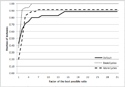
(a) Performance profile for Set 118_15.

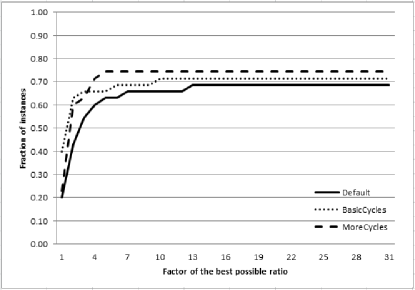
(b) Performance profile for Set 118_9G.

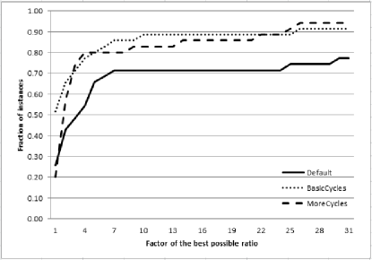
(c) Performance profile for Set 118_15_6.

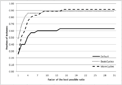
(d) Performance profile for Set 118_15_16.

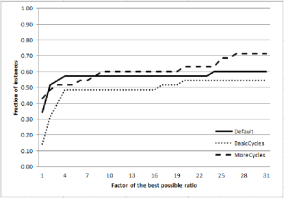
(e) Performance profile for Set 300_5.

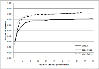
(f) Performance profile for all the instances.

Figure 1: Performance profiles for test instances.

6.3 Sensitivity Analysis

Previous literature on the DC-OTS demonstrates that significant cost savings can be achieved by switching off only a few lines (Fisher et al. 2008, Wu and Cheung 2013). However, the optimal solutions obtained by the integer program turn off a significantly larger number of lines than suggested by previous studies. Specifically, the average number of lines turned off in the optimal solutions to the 118-bus instances is 42, and the maximum number turned off is 57. For the 300-bus instances, an average of 85 lines are turned off in the optimal solutions, with a maximum of 107. This surprising result is a consequence of our observation that there are many optimal or near-optimal topologies for the DC-OTS. To demonstrate the impact of switching off fewer lines than suggested by the optimal solution to the integer program, we performed a sensitivity analysis of the cost versus the number of lines $N$ that are allowed to be switched off.

In this analysis, we chose one instance from each of the five sets whose optimal solution had a large number of lines switched off (41, 38, 41, 48, 91, respectively - refered to as instances (a), (b), (c), (d), (e) henceforth) and solved a number of DC-OTS instances with the cardinality constraint:

$$\sum_{(i,j)\in\mathcal{L}}x_{ij}\geq|\mathcal{L}|-N$$ (34)

added to the formulation. Here, $N$ is the switching budget, that is, the number of lines allowed to be switched off (note that $N=0$ corresponds to DC-OPF). We experimented with different $N$ values and the results are given in Figures 2(a)-2(e). We make the following observations:

• DC-OPF versions of instances (a), (c), (d) and (e) are infeasible.

• Once a particular instance becomes feasible, increasing the switching budget has a significant effect on the objective value for the first few lines (especially, for instances (b), (d) and (e)).

• Nevertheless, the full cost benefit can only be realized by switching off several lines.

• Switching off 11 lines is enough for 118-bus instances (a), (b), (c), (d) to achieve the maximum cost benefit (just seven lines are needed for instance (b)).

• For the 300-bus instance, switching off 15 lines yields nearly the maximum cost benefit.

• The LP relaxation value is not affected by the switching budget.

Our results support the observation that most, although not all, of the cost benefits in transmission switching can be realized by switching off only a few lines. This has a positive impact on the robustness of the network. In our experience, the MIP instances with cardinality constraints were more time consuming to solve that without the cardinality constraint. For example the two instances which had the largest number of switched off lines in the optimal solutions we found (the 118-bus instance with 57 lines switched off and the 300-bus instance with 107 lines switched off) could not be solved in one hour for most switching budgets. Our observation that the LP relaxation value is not affected by the switching budget may help explain this. Since the optimal IP value is larger for smaller switching budgets, the LP relaxation gap is larger for these instances.

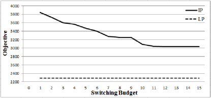
(a) An instance from Set 118_15.

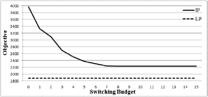
(b) An instance from Set 118_9G.

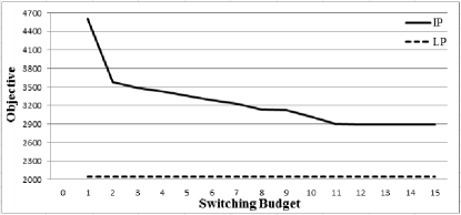
(c) An instance from Set 118_15_6.

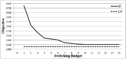
(d) An instance from Set 118_15_16.

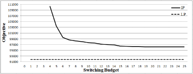
(e) An instance from Set 300_5.

Figure 2: Evolution of objective function (IP) and linear programming relaxation (LP) with respect to different switching budgets for five instances.

7 Conclusions

In this paper, we propose new cycle-based formulations for the optimal power flow problem and the optimal transmission switching problems that use the DC approximation to the power flow equations. We characterize the convex hull of a cycle-induced substructure in the new formulation, which provides strong valid inequalities that we may add to improve the new formulation. We demonstrate that separating the new inequalities may be done in linear time for a fixed cycle. We conduct extensive experiments to show that the valid inequalities are very useful in reducing the size of the search tree and the computation time for the DC optimal transmission switching problem.

The inequalities we derive may be gainfully employed for any power systems problem that involves the addition or removal of transmission lines and for which the DC approximation to power flow is sufficient for engineering purposes. We will pursue the application of these inequalities to other important power systems planning and operations problems as a future line of research. Other future lines of research include the investigation of more complicated substructure of the new formulation, and engineering the cutting plane procedure to effectively solve larger-scale networks. As an example of studying more complicated substructures, one reviewer observed that the substructure we study does not involve flow balance constraints. Stronger relaxations could be obtained by separating cutting-planes using an extended formulation similar to (14) that includes flow balance constraints.

Appendix A Cycle Basis Algorithm

Proposition A.1.

Algorithm 5 works correctly.

Proof.

Without loss of generality, assume that the first $n-1$ rows of $A$ are selected such that no row permutation is necessary during LU decomposition. In the remaining of the proof, we will replace $PA$ with $A$ for brevity.

The LU decomposition of $A$ can be obtained by a sequence of Gaussian eliminations on $A$ as

$$\tilde{A}_{1}=\tilde{L}_{1}\cdot A,\;\;\tilde{A}_{2}=\tilde{L}_{2}\cdot\tilde{A}_{1},\dots,\;\;U=\tilde{A}_{n-1}=\tilde{L}_{n-1}\cdot\tilde{A}_{n-1},$$

where each matrix $\tilde{L}_{i}$ is an elementary row operation that adds or subtracts multiples of the $i$-th row of $\tilde{A}_{i-1}$ to other rows to make the $i$-th column of $\tilde{A}_{i-1}$ the $i$-th unit vector. Consider a nonzero entry $a_{i1}$ of $A$. Since $a_{11},a_{i1}\in\{+1,-1\}$, the row operation only adds $+1$ or $-1$ copy of row $1$ to row $i$, that is, the first column of $\tilde{L}_{1}$ only contains $0,\pm 1$. Also, after eliminating $a_{i1}$, row $i$ of $A_{1}$ will either be all zero, or contain exactly one $1$ and one $-1$. In other words, $A_{1}$ is an arc-node incidence matrix for a new digraph $G_{1}=(V,E_{1})$. Since rank$(A)=n-1$, we have rank$(\tilde{A}_{1})=n-1$, which implies the new digraph $G_{1}$ is connected. Repeating this argument for each subsequent round of Gaussian elimination, we have that $U$ is an incidence matrix of the connected digraph $G_{n-1}$ with $n-1$ arcs, which implies $G_{n-1}$ is a spanning tree of the node set $V$. Denote the first $n-1$ rows of $U$ as $U_{1}$. The last $m-n+1$ rows of $U$ are zeros.

Denote $A=\begin{bmatrix}A_{1}\\ A_{2}\end{bmatrix}$ where $A_{1}$ is the first $n-1$ rows of $A$ and represents a spanning tree ${T}$ in the original graph ${G}$. Note that the rows of $A_{1}$ are linearly independent. Let us first carry out the LU decomposition of $A_{1}$ to get $A_{1}=L_{1}U_{1}$. In fact, $U_{1}$ represents a spanning tree, say ${T^{\prime}}$, on a new graph ${G^{\prime}}=(V,E^{\prime})$. Note that the entries of $L_{1}$ are precisely the negative of the pivots in Gaussian elimination and hence, they are $\pm 1$. Moreover, we can interpret the rows of $L_{1}$ indexed by the edges in ${T}$ and columns indexed by the edges in ${T^{\prime}}$. In particular, the elements of row $(i,j)\in{T}$ represent the unique path in ${T^{\prime}}$ going from $i$ to $j$.

Claim A.1.

A path in ${T}$ can be mapped to a path in ${T^{\prime}}$ by post-multiplication of $L_{1}$ and this transformation is unique.

Proof.

Let us consider a path $p$ in ${T}$ as a row vector where +1 (-1) means an arc is traversed in forward (backward) direction and 0 means that arc is not part of the path. Define $p^{\prime}=pL_{1}$. We claim that the row vector $p^{\prime}$ is a path in ${T^{\prime}}$. Let us traverse the path $p$ in terms of the edges in ${T^{\prime}}$. In particular, we weight the rows of $\mathcal{T}$ corresponding to $(i,j)$ with the value of that edge in the path $p$. In other words, for each arc $(i,j)$ in the path, we traverse the path from $i$ to $j$ in $\mathcal{T^{\prime}}$. But, this gives a path in $\mathcal{T^{\prime}}$. Finally, this transformation is unique since the path joining two nodes in a tree is unique. ∎

Now, consider $A^{\prime}=\begin{bmatrix}U_{1}\\ A_{2}\end{bmatrix}$. We continue LU decomposition on $A^{\prime}$ to obtain $A^{\prime}=\begin{bmatrix}U_{1}\\ A_{2}\end{bmatrix}=\begin{bmatrix}I&0\\ L_{2}&I\end{bmatrix}\begin{bmatrix}U_{1}\\ 0\end{bmatrix}$. In particular, we have $A_{2}=L_{2}U_{1}$. Since the rows of $U_{1}$ are linearly independent and $U_{1}$ defines a tree, the elements of $A_{2}$ can be traced via a unique path in ${T^{\prime}}$. In fact, the paths are exactly $L_{2}$ in the new network. If the paths in $L_{2}$ are traced backwards, we obtain cycles in ${G^{\prime}}$. Hence, $\begin{bmatrix}-L_{2}&I\end{bmatrix}$ is a cycle basis in ${G^{\prime}}$.

At this point, we can write $A=LU$ where

$$L=\begin{bmatrix}L_{1}&0\\ 0&I\end{bmatrix}\begin{bmatrix}I&0\\ L_{2}&I\end{bmatrix}\text{ and }L^{-1}=\begin{bmatrix}L_{1}^{-1}&0\\ -L_{2}L_{1}^{-1}&I\end{bmatrix}$$

Finally, we claim that $C_{b}=\begin{bmatrix}-L_{2}L_{1}^{-1}&I\end{bmatrix}$ is a cycle basis in ${G}$. Let us first focus on the system $L_{2}=ML_{1}$. Recall that the rows of $L_{2}$ are paths in ${G^{\prime}}$. We claim that the rows of $M$ are the corresponding paths in $G$. Using Claim A.1, we know that post-multiplication of a path in $G$ by $L_{1}$ gives a path in $G^{\prime}$. But, since $L_{1}$ is invertible, $M=L_{2}L_{1}^{-1}$ is the unique solution and therefore, the rows of $M$ should represent paths in ${G}$. Then, by tracing the paths in $M$ backwards, we obtain cycles in ${G}$. Therefore, $\begin{bmatrix}-L_{2}L_{1}^{-1}&I\end{bmatrix}$ is a cycle basis in ${G}$. ∎

Note that we do not need to explicitly invert $L$ to obtain $L^{-1}$. In fact, LU decomposition produces $L^{-1}$. Hence, it is computationally efficient to find cycle basis using Algorithm 5.

References

- Cpl (2011) 2011. User’s Manual for CPLEX Version 12.4. IBM.
- Barahona and Mahjoub (1986) Barahona, F., A.R. Mahjoub. 1986. On the cut polytope. Math. Program. 36 157–173.
- Barrows et al. (2012) Barrows, C., S. Blumsack, R. Bent. 2012. Computationally efficient optimal transmission switching: Solution space reduction. Power and Energy Society General Meeting, 2012 IEEE. 1–8. doi:10.1109/PESGM.2012.6345550.
- Barrows et al. (2014) Barrows, C., S. Blumsack, P. Hines. 2014. Correcting optimal transmission switching for AC power flows. 47th Hawaii International Conference on System Sciences (HICSS). 2374–2379.
- Bienstock and Mattia (2007) Bienstock, D., S. Mattia. 2007. Using mixed-integer programming to solve power grid blackout problems. Discret. Optim. 4(1) 115–141. doi:10.1016/j.disopt.2006.10.007.
- Blumsack (2006) Blumsack, S.A. 2006. Network topologies and transmission investment under electric-industry restructuring. Ph.D. thesis, Carnegie Mellon University, Pittsburgh, Pennsylvania.
- Bollobás (2002) Bollobás, B. 2002. Modern Graph Theory. Springer.
- Coffrin et al. (2014) Coffrin, C., H. Hijazi, P. Van Hentenryck, K. Lehmann. 2014. Primal and dual bounds for optimal transmission switching. Power Systems Computation Conference (PSCC). Poland.
- Dolan and Moré (2002) Dolan, E.D., J.J. Moré. 2002. Benchmarking optimization software with performance profiles. Math. Program. Ser. A 91 201–213.
- Ferreira et al. (1996) Ferreira, C.E., A. Martin, C.C. de Souza, R. Weismantel, L.A. Wolsey. 1996. Formulations and valid inequalities for the node capacitated graph partitioning problem. Math. Program. 74 247–266.
- Fisher et al. (2008) Fisher, E.B., R.P. O’Neill, M.C. Ferris. 2008. Optimal transmission switching. IEEE Transactions on Power Systems 1346–1355.
- Fuller et al. (2012) Fuller, J.D., R. Ramasra, A. Cha. 2012. Fast heuristics for transmission-line switching. IEEE Transactions on Power Systems 27(3) 1377–1386. doi:10.1109/TPWRS.2012.2186155.
- Garey and Johnson (1990) Garey, M.R., D.S. Johnson. 1990. Computers and Intractability; A Guide to the Theory of NP-Completeness. W. H. Freeman & Co., New York, NY, USA.
- Hariharan et al. (2008) Hariharan, Ramesh, Telikepalli Kavitha, Kurt Mehlhorn. 2008. Faster algorithms for minimum cycle basis in directed graphs. SIAM Journal on Computing 38(4) 1430–1447.
- Hedman et al. (2010) Hedman, K.W., M.C. Ferris, R.P. O’Neill, E.B. Fisher, S.S. Oren. 2010. Co-optimization of generation unit commitment and transmission switching with n-1 reliability. IEEE Transactions on Power Systems 25(2) 1052–1063. doi:10.1109/TPWRS.2009.2037232.
- Hedman et al. (2009) Hedman, K.W., R.P. O’Neill, E.B. Fisher, S.S. Oren. 2009. Optimal transmission switching with contingency analysis. IEEE Transactions on Power Systems 24(3) 1577–1586. doi:10.1109/TPWRS.2009.2020530.
- Hedman et al. (2011) Hedman, K.W., S.S. Oren, R.P. O’Neill. 2011. A review of transmission switching and network topology optimization. Power and Energy Society General Meeting, 2011 IEEE. 1–7. doi:10.1109/PES.2011.6039857.
- Hijazi et al. (2013) Hijazi, H., C. Coffrin, P. V. Hentenryck. 2013. Convex quadratic relaxations of nonlinear programs in power systems. Technical report, NICTA. http://www.optimization-online.org/DBHTML/2013/09/4057.html.
- Kavitha et al. (2009) Kavitha, T., C. Liebchen, K. Mehlhorn, D. Michail, R. Rizzi, T. Ueckerdt, K. Zweig. 2009. Cycle bases in graphs: Characterization, algorithms, complexity, and applications. Computer Science Review 3 199–243.
- Khodaei et al. (2010) Khodaei, A., M. Shahidehpour, S. Kamalinia. 2010. Transmission switching in expansion planning. IEEE Transactions on Power Systems 25(3) 1722–1733. doi:10.1109/TPWRS.2009.2039946.
- Lehmann et al. (2014) Lehmann, K., A. Grastien, P. Van Hentenryck. 2014. The complexity of DC-Switching problems. Technical report, NICTA.
- O’Neill et al. (2005) O’Neill, R., R. Baldick, U. Helman, M. Rothkopf, J. Stewart. 2005. Dispatchable transmission in RTO markets. IEEE Transactions on Power Systems 20(1) 171–179.
- Padberg (1973) Padberg, M. 1973. On the facial structure of set packing polyhedra. Math. Program. 5 199–215.
- Soroush and Fuller (2014) Soroush, M., J.D. Fuller. 2014. Accuracies of optimal transmission switching heuristics based on dcopf and acopf. IEEE Transactions on Power Systems 29(2) 924–932. doi:10.1109/TPWRS.2013.2283542.
- Van Vyve (2005) Van Vyve, M. 2005. The continuous mixing polyhedron. Math. Oper. Res. 30 441–452.
- Villumsen and Philpott (2012) Villumsen, J. C., A. B. Philpott. 2012. Investment in electricity networks with transmission switching. European Journal of Operational Research 222 377–385.
- Villumsen et al. (2013) Villumsen, J.C., G. Bronmo, A.B. Philpott. 2013. Line capacity expansion and transmission switching in power systems with large-scale wind power. IEEE Transactions on Power Systems 28(2) 731–739. doi:10.1109/TPWRS.2012.2224143.
- Wu and Cheung (2013) Wu, J., K.W. Cheung. 2013. On selection of transmission line candidates for optimal transmission switching in large power networks. Power and Energy Society General Meeting (PES), 2013 IEEE. 1–5. doi:10.1109/PESMG.2013.6672912.