Nonlinear GARCH model and $1/f$ noise

Abstract

Auto-regressive conditionally heteroskedastic (ARCH) family models are still used, by practitioners in business and economic policy making, as a conditional volatility forecasting models. Furthermore ARCH models still are attracting an interest of the researchers. In this contribution we consider the well known GARCH(1,1) process and its nonlinear modifications, reminiscent of NGARCH model. We investigate the possibility to reproduce power law statistics, probability density function and power spectral density, using ARCH family models. For this purpose we derive stochastic differential equations from the GARCH processes in consideration. We find the obtained equations to be similar to a general class of stochastic differential equations known to reproduce power law statistics. We show that linear GARCH(1,1) process has power law distribution, but its power spectral density is Brownian noise-like. However, the nonlinear modifications exhibit both power law distribution and power spectral density of the $1/f^{\beta}$ form, including $1/f$ noise.

1 Introduction

Forecasting volatility opens up a possibility to make better-informed decisions. Thus this problem is of high interest to the practitioners in business and economic policy making as well as to the scientific community. The auto-regressive conditionally heteroskedastic (ARCH) model and its generalization, known as GARCH, were proposed exactly for this purpose [1, 2]. Since then numerous modifications of the seminal models proposed by Engle and Bollerslev were introduced to serve varying purposes: from financial market to macroeconomic modeling (see [3] for a long list of the ARCH family models). Our particular interest, in the context of this paper, lies in the continuous-time GARCH model (COGARCH, see [4, 5, 6, 7]) and nonlinear variations of GARCH, such as NGARCH [8, 9] or MARCH [10].

In order to evaluate the suitability of a given model one should compare the features of the time series produced by the model with the actual empirical data. It is known that high frequency time series of financial data exhibit some universal statistical properties. Vast amounts of historical stock price data around the world have helped to establish a variety of so-called stylized facts [11, 12, 13, 14, 15, 16, 17, 18, 19, 20] corresponding to the statistical signatures of financial processes. One of the stylized facts concerns with autocorrelation function, or, equivalently, power spectral density (PSD) of the time series. There is empirical evidence that trading activity, trading volume, and volatility are stochastic variables with the long-range correlation [21, 22, 23] leading to $1/f$ type PSD. Successful models should reproduce as many stylized facts as possible. However, the $1/f$ type PSD is not accounted for in some widely used models, such as ARCH family models. Therefore, it would be useful to examine under which conditions power law PSD may be observed in GARCH(1,1) and in nonlinear modifications of GARCH(1,1) models.

Power law statistics and especially $1/f$ noise are rather ubiquitous phenomena observed in many different fields of science ranging from natural phenomena to computer networks and financial markets [24, 25, 26, 27, 28, 29]. Since the discovery of $1/f$ noise numerous models and theories have been proposed, for a recent review see [30]. A class of nonlinear stochastic differential equations (SDEs) exhibiting power law probability density function (PDF) and power law PSD in a wide region of frequencies has been derived in [31, 32, 33, 34] starting from the point process model. Such nonlinear SDEs have been used to describe signals in socio-economical systems [35, 36].

Usually ARCH family models are calibrated by retro-fitting historical data and thus may replicate patterns observed in the past [37]. Yet other approaches are also possible. For example, one may consider comparing them to successful models from other frameworks. In this paper we compare GARCH(1,1) and its nonlinear modifications to nonlinear stochastic differential equations generating signals with power law PSD.

This work is organized as follows: in Section 2 we briefly introduce a class of nonlinear SDEs reproducing $1/f$ noise; in Section 3 we show that power law distributions with varying exponents may be obtained from GARCH(1,1) process; in Section 4 we consider a nonlinear modifications of GARCH(1,1) process using which we reproduce $1/f$ noise. Section 5 summarizes our work.

2 Stochastic differential equations generating signals with $1/f$ noise

The nonlinear SDEs generating signals with power law steady state PDF and $1/f^{\beta}$ PSD have been previously derived in Refs. [31, 32, 33]. The general expression for the proposed class of Itô SDEs is given by

$$\mathrm{d}x=\sigma^{2}\left(\eta-\frac{1}{2}\lambda\right)x^{2\eta-1}\mathrm{d}t+\sigma x^{\eta}\mathrm{d}W_{t}\,.$$ (1)

In the above $x$ is the signal, $\eta\neq 1$ is the exponent of a power law multiplicative noise, $\lambda$ defines the exponent of the power law steady state PDF of the signal, while $W_{t}$ is the standard Wiener process (one dimensional Brownian motion) and $\sigma$ is a scaling constant determining the intensity of noise. The nonlinear SDE (1) assumes the simplest form of the multiplicative noise term, $\sigma x^{\eta}\mathrm{d}W_{t}$, although it may take other forms as long as $\eta$ is the largest power of $x$ for large values of $x$ [33, 35]. Such nonlinear SDEs have been used to describe signals in socio-economical systems [35, 36]. In Refs. [38, 39] a nonlinear SDE similar to the one given by Eq. (1) was derived by starting from a simple agent-based herding model, thus providing agent-based reasoning for this class of SDEs.

The steady state PDF of Eq. (1) has a power law form $p(x)\sim x^{-\lambda}$ with the exponent $\lambda$. If $\lambda>1$ then $p(x)$ diverges as $x\rightarrow 0$, therefore the diffusion of the stochastic variable $x$ should be restricted from the side of small values. This can be achieved by modifying Eq. (1). The simplest restriction of the diffusion is produced by the reflective boundary conditions at the minimum value $x=x_{\mathrm{min}}$ and the maximum value $x=x_{\mathrm{max}}$. Alternatively, one can modify Eq. (1) to get rapidly decreasing steady state PDF when the stochastic variable $x$ acquires values outside of the interval $[x_{\mathrm{min}},x_{\mathrm{max}}]$. For example, the steady state PDF

$$p(x)\sim\frac{1}{x^{\lambda}}\exp\left(-\frac{x_{\mathrm{min}}^{m}}{x^{m}}-\frac{x^{m}}{x_{\mathrm{max}}^{m}}\right)$$ (2)

with $m>0$ has a power law form inside of the interval $x_{\mathrm{min}}\ll x\ll x_{\mathrm{max}}$ and exponential cut-offs are present outside of this interval. Exponentially restricted diffusion is generated by the SDE

$$\mathrm{d}x=\sigma^{2}\left[\eta-\frac{1}{2}\lambda+\frac{m}{2}\left(\frac{x_{\mathrm{min}}^{m}}{x^{m}}-\frac{x^{m}}{x_{\mathrm{max}}^{m}}\right)\right]x^{2\eta-1}\mathrm{d}t+\sigma x^{\eta}\mathrm{d}W_{t}$$ (3)

which differs from Eq. (1) only by a couple of additional terms in the drift part of SDE.

One can estimate the PSD of the signals generated by the SDE (1) by using the approximate scaling properties of the signals [40]. The Wiener process scales as $\mathrm{d}W_{at}=a^{1/2}\mathrm{d}W_{t}$, thus by changing the variable $x$ in Eq. (1) to a scaled variable $x_{s}=ax$ or by introducing the scaled time $t_{s}=a^{2(\eta-1)}t$ one obtains exactly the same SDE. This feature indicates that the change of the scale of the stochastic variable $x$ and the change of the time scale are statistically equivalent. Using the transition probability (the conditional probability that at time $t$ the signal has value $x^{\prime}$ with the condition that at time $t=0$ the signal had the value $x$) this equivalence may be mathematically expressed as

$$aP(ax^{\prime},t|ax,0)=P(x^{\prime},a^{\mu}t|x,0)\,,$$ (4)

with the exponent $\mu$ being equal to $2(\eta-1)$. The discussed scaling property Eq. (4) as well as power law form of the steady state PDF $p(x)\sim x^{-\lambda}$ lead to the PSD with power law behavior $S(f)\sim f^{-\beta}$, which is observed in a wide range of frequencies. The power law exponent of the PSD is given by [40]

$$\beta=1+\frac{\lambda-3}{2(\eta-1)}\,.$$ (5)

The restrictions imposed on diffusion at $x=x_{\mathrm{min}}$ and $x=x_{\mathrm{max}}$ makes the scaling relationship Eq. (4) only approximate. This limits the power law part of the PSD to a certain finite range of frequencies $f_{\mathrm{min}}\ll f\ll f_{\mathrm{max}}$. Note, that power law behavior $1/f^{\beta}$ of the PSD for all frequencies is physically impossible, because the total power of the signal then would be infinite. Therefore, it is natural to consider signals with the power law PSD in a limited range of frequencies. The frequency range for the PSD of the signal generated by solving SDE (4) was estimated in Ref. [40] as

$$\sigma^{2}x_{\mathrm{min}}^{2(\eta-1)} \ll 2\pi f\ll\sigma^{2}x_{\mathrm{max}}^{2(\eta-1)},\qquad\eta>1,$$ (6)

$$\sigma^{2}x_{\mathrm{max}}^{-2(1-\eta)} \ll 2\pi f\ll\sigma^{2}x_{\mathrm{min}}^{-2(1-\eta)},\qquad\eta<1.$$

From Eq. (6) it is evident that the width of the frequency range can be increased by increasing the ratio between the minimum and the maximum diffusion restriction boundary positions $x_{\mathrm{max}}/x_{\mathrm{min}}$. In addition, the width also depends on the multiplicative noise exponent $\eta$. Namely, the width is zero if $\eta=1$ and increases with increasing $|\eta-1|$ [34].

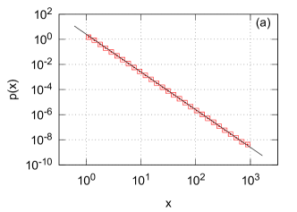
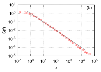
Figure 1: Statistical properties, PDF (a) and PSD (b), obtained by numerically solving SDE (1) (red squares). In the numerical computation we have used the reflective boundaries placed at $x_{\mathrm{min}}$ and $x_{\mathrm{max}}$. Black curves show power law approximations (a) $x^{-3}$ for numerically obtained PDF and (b) $1/f$ for the PSD. The following parameter values were used: $\eta=2$, $\lambda=3$, $x_{\mathrm{min}}=1$, $x_{\mathrm{max}}=10^{3}$, $\sigma=1$.

With $\lambda=3$, from Eq. (5) we obtain $\beta=1$ and SDE (1) should generate a signal exhibiting $1/f$ noise. This case with $\eta=2$ is shown in Fig. 1. In numerical computation we have used a modified Euler-Maruyama approximation (the original Euler-Maruyama approximation is described in [41]) with a variable time step which decreases with the larger values of $x$, as is described in [31, 32]. We find a good agreement of the numerical results with analytical predictions. Though the range of frequencies with $S(f)\sim 1/f$ is much narrower than expected, $1\ll f\ll 10^{3}$ versus $1\ll f\ll 10^{6}$ predicted by Eq. (6). This discrepancy arises because Eq. (6) is only a qualitative estimation. To obtain a more precise values of limiting frequencies one needs to use more precise scaling properties of the nonlinear SDE.

3 GARCH(1,1) process and stochastic differential equations

Almost half a century ago Mandelbrot, Fama and others proposed an idea that volatility fluctuations might be responsible for the fluctuating nature of price change (return) dynamics [42, 43, 44]. Actually intermittency of return time series is usually associated with localized burst in volatility and thus frequently referred to as volatility clustering [27, 45, 46, 47]. It was proven that modeling temporal dynamics of second-order moment, known as heteroskedasticity [1], may allow better performing option-price models [48, 49, 50].

In his seminal article [1] R. F. Engle laid foundations to the autoregressive conditional heteroskedasticity (ARCH) models by proposing to split a heteroskedastic variable $z$ (e.g., return) into a stochastic part $\omega_{t}$ and time dependent volatility (standard deviation) $\sigma_{t}$,

$$z_{t}=\sigma_{t}\omega_{t}\,.$$ (7)

Stochastic part $\omega_{t}$ may follow any distribution, but a common choice is the Gaussian distribution, though other distributions such as the $q$-Gaussian distribution might be also considered [51, 52]. In this paper we will use the Gaussian distribution with zero mean $\langle\omega_{t}\rangle=0$ and unit variance $\langle\omega_{t}^{2}\rangle=1$. As the process modeling the evolution of the standard deviation time series $\sigma_{t}$ we choose GARCH(1,1) process, which is defined as an iterative equation of the following form:

$$\sigma_{t}^{2}=a+bz_{t-1}^{2}+c\sigma_{t-1}^{2}\,.$$ (8)

Using Eq. (7) the GARCH(1,1) process can be written as

$$\sigma_{t}^{2}=a+b\sigma_{t-1}^{2}\omega_{t-1}^{2}+c\sigma_{t-1}^{2}\,.$$ (9)

GARCH(1,1) process can be approximated as a continuous time SDE by considering the diffusion limit of this process [4, 5, 6, 7]. Usually the parameters of the GARCH process are obtained by retro-fitting empirical data and thus the actual values of the parameters $a$, $b$ and $c$ are tied to a particular discretization time step. Taking this into account let us rewrite the above as [5]

$$\sigma_{kh,h}^{2} = a_{h}+b_{h}\sigma_{(k-1)h,h}^{2}\omega_{(k-1)h,h}^{2}+c_{h}\sigma_{(k-1)h,h}^{2}$$ (10)

$$= \sigma_{(k-1)h,h}^{2}+a_{h}-(1-b_{h}-c_{h})\sigma_{(k-1)h,h}^{2}+b_{h}\sigma_{(k-1)h,h}^{2}\left(\omega_{(k-1)h,h}^{2}-1\right)\,.$$

Here $h$ is a time series discretization period ($t=kh$, where $k=1,2,3,\ldots$), while subscripts indicate that the parameters depend on $h$. Assuming that $h$ is infinitesimally small, $h\rightarrow 0$ we introduce the continuous time parameters $A$, $B$ and $C$ related to the parameters $a_{h}$, $b_{h}$ and $c_{h}$ by the equations [5]

$$a_{h}=Ah,\quad 1-b_{h}-c_{h}=Ch,\quad 2b_{h}^{2}=B^{2}h\,.$$ (11)

Note, that the parameters $A$, $B$, $C$ do not depend on $h$. Using Eq. (11) we can rewrite Eq. (10) as

$$\sigma_{kh,h}^{2}=\sigma_{(k-1)h,h}^{2}+\left(A-C\sigma_{(k-1)h,h}^{2}\right)h+|B|\sqrt{\frac{h}{2}}\sigma_{(k-1)h,h}^{2}\left(\omega_{(k-1)h,h}^{2}-1\right)\,.$$ (12)

The stochastic variable $\omega_{(k-1)h,h}^{2}-1$ we approximate as a normally distributed stochastic variable with zero mean and variance equal to $2$, since $\langle\omega^{2}-1\rangle=0$ and $\langle(\omega^{2}-1)^{2}\rangle=k_{\omega}-1=2$. This gives

$$\sigma_{kh,h}^{2}=\sigma_{(k-1)h,h}^{2}+\left(A-C\sigma_{(k-1)h,h}^{2}\right)h+|B|\sigma_{(k-1)h,h}^{2}\sqrt{h}\varepsilon_{k}\,,$$ (13)

where $\varepsilon_{k}$ is a normally distributed stochastic variable with zero mean and unit variance. Note, that the last equation has the form of a difference equation, similar to the Euler-Marujama approximation used to numerically solve SDEs. Thus by taking the small time step limit $h\rightarrow 0$ one can obtain the SDE for the variable $y_{kh,h}=\sigma_{kh,h}^{2}$ from Eq. (13):

$$\mathrm{d}y=(A-Cy)\mathrm{d}t+|B|y\mathrm{d}W_{t}\,.$$ (14)

This equation can be written in the form

$$\mathrm{d}y=B^{2}\left(1-\frac{1}{2}\lambda+\frac{1}{2}\frac{y_{\mathrm{min}}}{y}\right)y\mathrm{d}t+|B|y\mathrm{d}W_{t}\,,$$ (15)

where

$$\lambda = 2+\frac{2C}{B^{2}}=2+\frac{1-b_{h}-c_{h}}{b_{h}^{2}}\,,\qquad y_{\mathrm{min}}=\frac{2A}{B^{2}}=\frac{a}{b_{h}^{2}}\,.$$ (16)

The SDE (15) is a special case of the SDE (1) with $\eta=1$. As is discussed in Section 2, steady state PDF $p(y)$ thus should have power law tail with the exponent $\lambda$, $p(y)\sim y^{-\lambda}$. Analytical prediction Eq. (5) for the power law exponent in the PSD diverges, but it is worth to note that the SDE (15) is similar to geometric Brownian motion, PSD of which has the power law exponent $\beta=2$.

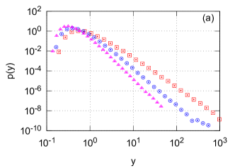
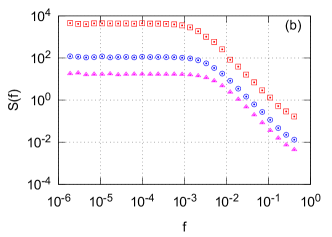
Figure 2: Statistical properties, PDF (a) and PSD (b), of numerically evaluated linear GARCH(1,1) process Eq. (8). The GARCH(1,1) process parameters were set as follows: $a=0.015$, $b=0.1$, $c=0.89$ (red squares), $0.88$ (blue circles) and $0.87$ (magenta triangles).

The PDF and the PSD of the time series numerically obtained using GARCH(1,1) process, Eq. (8), are shown in Fig. 2. The analytical predictions of the power law exponents in the PDF and the PSD are in good agreement with the numerical results.

4 Nonlinear GARCH(1,1) process generating signals with $1/f$ noise

The mathematical form of Eq. (5) suggests that it is possible to obtain other values of the power law exponent $\beta$ as long as $\eta\neq 1$. In our previous work we have shown that $\eta>1$ cases work very well for the modeling of high-frequency trading activity as well as high-frequency absolute returns of the financial markets [53, 35, 54], although theoretically $\eta<1$ is also possible [34]. One can obtain the $\eta>1$ case by considering the following modifications of GARCH(1,1) process:

$$\sigma_{t}^{2} = a+b\sigma_{t-1}^{\mu}\omega_{t-1}^{\mu}+c\sigma_{t-1}^{2}\,,$$ (17)

where $\mu>2$ is an odd integer, and

$$\sigma_{t}^{2}=a+b\sigma_{t-1}^{\mu}|\omega_{t-1}|^{\mu}+\sigma_{t-1}^{2}-c\sigma_{t-1}^{\mu}\,,$$ (18)

where $\mu$ may be any positive real number. Nonlinear GARCH model of a similar form was considered by Engle and Bollerslev in [8]. Nonlinear model proposed by Engle and Bollerslev had a form of Eq. (17), but absolute value of $\omega_{t-1}$ was taken prior to raising it to a generalized power $\mu$. Engle and Bollerslev found that $\mu\lessapprox 2$ for most empirical timeseries they have considered. Another take at nonlinear GARCH model can be found in work by Higgins and Bera [9], although they considered dynamics not of the standard deviation (as we do), but of the higher order moment, $\sigma_{t}^{\mu}$. Note, that the last two terms in Eq. (18) can be seen as the first two terms in the power series expansion of a more general function of standard deviation $f(\sigma_{t})$. In contrast to Eq. (8) for the GARCH(1,1) process, Eqs. (17) and (18) do not ensure the positivity of $\sigma_{t}^{2}$. In order to avoid negative values of $\sigma_{t}^{2}$ we consider Eqs. (17) and (18) together with a reflective boundary at $\sigma_{t}^{2}=0$.

Let us first consider the diffusion limit of Eq. (17). We proceed similarly as in Section 3. Taking into account the relation to physical time via time series sampling, this iterative equation may be rewritten as follows:

$$\sigma_{kh,h}^{2}=\sigma_{(k-1)h,h}^{2}+a_{h}-(1-c_{h})\sigma_{(k-1)h,h}^{2}+b_{h}\sigma_{(k-1)h,h}^{\mu}\omega_{(k-1)h,h}^{\mu}\,.$$ (19)

Assuming that the time discretization period $h$ is infinitesimally small, $h\rightarrow 0$, we can introduce the coefficients $A$, $B$ and $C$ via the equations

$$a_{h}=Ah\,,\qquad 1-c_{h}=Ch\,,\qquad\langle\omega^{2\mu}\rangle b_{h}^{2}=B^{2}h$$ (20)

and rewrite Eq. (19) as

$$\sigma_{kh,h}^{2}=\sigma_{(k-1)h,h}^{2}+\left(A-C\sigma_{(k-1)h,h}^{2}\right)h+|B|\sqrt{\frac{h}{\langle\omega^{2\mu}\rangle}}\sigma_{(k-1)h,h}^{\mu}\omega_{(k-1)h,h}^{\mu}\,.$$ (21)

We approximate the stochastic variable $\omega_{(k-1)h,h}^{\mu}$ as a normal stochastic variable with zero mean (given that $\mu$ is odd) and variance $\langle\omega^{2\mu}\rangle$. This gives

$$\sigma_{kh,h}^{2}=\sigma_{(k-1)h,h}^{2}+\left(A-C\sigma_{(k-1)h,h}^{2}\right)h+|B|\sqrt{h}\sigma_{(k-1)h,h}^{\mu}\varepsilon_{k}\,,$$ (22)

where $\varepsilon_{k}$ is a normally distributed stochastic variable with zero mean and unit variance. By taking the small time step limit $h\rightarrow 0$, one can obtain the SDE for the variable $y_{kh,h}=\sigma_{kh,h}^{2}$ from Eq. (22):

$$\mathrm{d}y=\left(\frac{A}{y^{\mu-1}}-\frac{C}{y^{\mu-2}}\right)y^{\mu-1}\mathrm{d}t+|B|y^{\frac{\mu}{2}}\mathrm{d}W_{t}\,.$$ (23)

By introducing the parameters

$$y^{(1)} = \left(\frac{2A}{(\mu-1)B^{2}}\right)^{\frac{1}{\mu-1}}\,,\qquad y^{(2)}=\left(\frac{2C}{(\mu-2)B^{2}}\right)^{\frac{1}{\mu-2}}$$ (24)

Eq. (23) can be rewritten as

$$\mathrm{d}y=B^{2}\left[\frac{1}{2}(\mu-1)\left(\frac{y^{(1)}}{y}\right)^{\mu-1}-\frac{1}{2}(\mu-2)\left(\frac{y^{(2)}}{y}\right)^{\mu-2}\right]y^{\mu-1}\mathrm{d}t+|B|y^{\frac{\mu}{2}}\mathrm{d}W_{t}\,.$$ (25)

From the Fokker-Planck equation corresponding to Eq. (25) one can obtain the steady state PDF $p(y)$ of the signal generated by Eq. (25). The steady state PDF $p(y)$ has a power law tail with the exponent $\lambda=\mu$, while $y^{(1)}$ and $y^{(2)}$ shape the exponential cutoff:

$$p(y)\sim\frac{1}{y^{\mu}}\exp\left[-\left(\frac{y^{(1)}}{y}\right)^{\mu-1}+\left(\frac{y^{(2)}}{y}\right)^{\mu-2}\right]\,.$$ (26)

Eq. (25) has the general form of SDE (1) with the parameters $\lambda=\mu$ and $\eta=\mu/2$. Thus the PSD of $y_{t}$ time series should have a frequency range with the power law behavior of the PSD $S(f)$ given by

$$S(f)\sim\frac{1}{f^{\beta}}\,,\qquad\beta=1+\frac{\mu-3}{\mu-2}\,.$$ (27)

Note, that we get $1/f$ PSD when $\mu=3$.

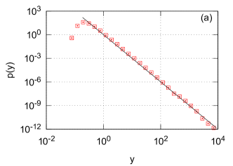
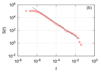
Figure 3: Statistical properties, PDF (a) and PSD (b), of numerically evaluated nonlinear GARCH process Eq. (17) with $\mu=3$ (red squares). Black curves show power law approximations (a) $x^{-3}$ for numerically obtained PDF and (b) $1/f$ for the PSD. Other nonlinear GARCH process parameters were set as follows: $a=10^{-6}$, $b=10^{-3}$, $c=1$.

The PDF and the PSD of the time series numerically obtained using Eq. (17) with $\mu=3$ are shown in Fig. 3. In the numerical calculations we used reflective boundary at $\sigma_{t}=0$. The analytical predictions of the power law exponents $\lambda=3$ in the PDF and $\beta=1$ in the PSD are in good agreement with the numerical results. With the chosen parameters in Eq. (17) we are able to reproduce $1/f$ spectrum over almost $4$ decades of frequency $f$, see Fig. 3(b).

Now let us consider the diffusion limit of Eq. (18). Eq. (18) may be rewritten by taking into account the relation to physical time:

$$\sigma_{kh,h}^{2}=\sigma_{(k-1)h,h}^{2}+a_{h}-c_{h}\sigma_{(k-1)h,h}^{\mu}+b_{h}\sigma_{(k-1)h,h}^{\mu}|\omega_{(k-1)h,h}|^{\mu}\,.$$ (28)

Approximating $|\omega_{(k-1)h,h}|^{\mu}$ as a normal stochastic variable with the mean $\bar{\omega}_{\mu}=\langle|\omega|^{\mu}\rangle$ and the variance $\hat{\omega}_{\mu}=\langle\left[|\omega|^{\mu}-\bar{\omega}_{\mu}\right]^{2}\rangle$ yields

$$\sigma_{kh,h}^{2}=\sigma_{(k-1)h,h}^{2}+a_{h}+\left(b_{h}\bar{\omega}_{\mu}-c_{h}\right)\sigma_{(k-1)h,h}^{\mu}+b_{h}\sigma_{(k-1)h,h}^{\mu}\sqrt{\hat{\omega}_{\mu}}\varepsilon_{k}\,.$$ (29)

Here $\varepsilon_{k}$ is a normally distributed stochastic variable with zero mean and unit variance. Assuming that the time discretization period $h$ is infinitesimally small, $h\rightarrow 0$, we can write Eq. (29) as

$$\sigma_{kh,h}^{2}=\sigma_{(k-1)h,h}^{2}+\left(A+C\sigma_{(k-1)h,h}^{\mu}\right)h+|B|\sqrt{h}\sigma_{(k-1)h,h}^{\mu}\varepsilon_{k}\,,$$ (30)

where the coefficients $A$, $B$ and $C$ are introduced via the equations

$$a_{h}=Ah\,,\qquad b_{h}\bar{\omega}_{\mu}-c_{h}=Ch\,,\qquad\hat{\omega}_{\mu}b_{h}^{2}=B^{2}h\,.$$ (31)

Note, that depending on the values of the parameters $b_{h}$ and $c_{h}$, the parameter $C$ can be negative as well as positive. By taking the small time step limit $h\rightarrow 0$ we can obtain the SDE for the variable $y_{kh,h}=\sigma_{kh,h}^{2}$:

$$\mathrm{d}y=\left(\frac{A}{y^{\mu-1}}+\frac{C}{y^{\frac{\mu}{2}-1}}\right)y^{\mu-1}\mathrm{d}t+|B|y^{\frac{\mu}{2}}\mathrm{d}W_{t}\,.$$ (32)

This equation can be written as

$$\mathrm{d}y=B^{2}\left[\frac{1}{2}(\mu-1)\left(\frac{y^{(1)}}{y}\right)^{\mu-1}+\frac{1}{2}\mathrm{sign}(C)\left(\frac{\mu}{2}-1\right)\left(\frac{y^{(3)}}{y}\right)^{\frac{\mu}{2}-1}\right]y^{\mu-1}\mathrm{d}t+|B|y^{\frac{\mu}{2}}\mathrm{d}W_{t}\,,$$ (33)

where

$$y^{(1)} = \left(\frac{2A}{(\mu-1)B^{2}}\right)^{\frac{1}{\mu-1}}\,,\qquad y^{(3)}=\left(\frac{4|C|}{\left(\mu-2\right)B^{2}}\right)^{\frac{2}{\mu-2}}\,.$$ (34)

The steady state PDF $p(y)$ of the signal generated by Eq. (33) has a power law tail with the exponent $\lambda=\mu$, while $y^{(1)}$ and $y^{(3)}$ shape the exponential cutoff:

$$p(y)\sim\frac{1}{y^{\mu}}\exp\left[-\left(\frac{y^{(1)}}{y}\right)^{\mu-1}-\mathrm{sign}(C)\left(\frac{y^{(3)}}{y}\right)^{\mu-2}\right]\,.$$ (35)

Eq. (33) has the general form of SDE (1) with the parameters $\lambda=\mu$ and $\eta=\mu/2$; the parameters are the same as as in the previous case, Eq. (17). Therefore, the PSD of $y_{t}$ time series should have a frequency range where Eq. (27) holds.

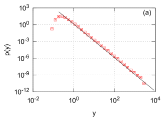
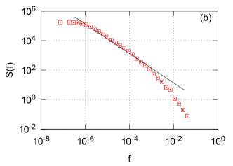
Figure 4: Statistical properties, PDF (a) and PSD (b), of numerically evaluated nonlinear GARCH process Eq. (18) with $\mu=3$ (red squares). Black curves show power law approximations (a) $x^{-3}$ for numerically obtained PDF and (b) $1/f$ for the PSD. Other nonlinear GARCH process parameters were set as follows: $a=10^{-6}$, $b=10^{-3}$, $c=2\sqrt{\frac{2}{\pi}}\cdot 10^{-3}\approx 1.595769\cdot 10^{-3}$. The chosen values of the parameters $b$ and $c$ lead to $C\approx 0$ and, consequently, $y^{(3)}\approx 0$ in the SDE (33) describing the diffusion limit of this nonlinear GARCh process.

The PDF and the PSD of the time series numerically obtained using Eq. (18) with $\mu=3$ are shown in Fig. 4. We have chosen the parameters $b$ and $c$ in Eq. (18) in such a way that the parameter $C$ given by Eq. (31) becomes zero. In the numerical calculations we used reflective boundary at $\sigma_{t}=0$ by setting $\sigma_{t}^{2}$ to zero when $\sigma_{t}^{2}$ becomes negative. The analytical predictions of the power law exponents $\lambda=3$ in the PDF and $\beta=1$ in the PSD are in good agreement with the numerical results. With the chosen parameters in Eq. (18) we are able to reproduce $1/f$ spectrum, but now over only $3$ decades of frequency $f$, see Fig. 4(b).

5 Conclusions

In summary, we have proposed two possible nonlinear modifications of a GARCH(1,1) process, Eqs. (17) and (18). Comparing the diffusion limit of the proposed nonlinear GARCH processes with the known nonlinear SDE (1) generating signals with $1/f^{\beta}$ PSD we obtain the conditions when the nonlinear GARCH processes yield $1/f^{\beta}$ PSD too. Numerical evaluation of Eqs. (17) and (18) with suitably chosen parameters confirms the presence of a wide power law region in the PSD of the time series. As should have been expected, the linear GARCH(1,1) process (8) does not reproduce $1/f$ spectrum. In addition to power law PSD, linear and nonlinear GARCH(1,1) processes resulted in power law distributions.

The results obtained in the paper are especially interesting as $1/f$ noise is often linked to a concept of long-range memory, which is considered to be one of the stylized facts of the financial markets as well as other socio-economic systems. The obtained results and proposed nonlinear GARCH processes should be useful for creation and application of ARCH family models that correctly reproduce the PSD of the financial time series as well.

References

- [1] R. Engle, Autoregresive conditional heteroscedasticity with estimates of the variance of united kingdom inflation, Econometrica 50 (4) (1982) 987–1008.
- [2] T. Bollerslev, Generalized autoregressive conditional heteroskedasticity, Journal of Econometrics 31 (1986) 307–327.
-
[3]
T. Bollerslev, Glossary to arch
(garch), CREATES Research Paper (2008).
URL http://dx.doi.org/10.2139/ssrn.1263250 - [4] D. B. Nelson, Arch models as diffusion approximations, Journal of Econometrics 45 (1-2) (1990) 7–38.
- [5] A. M. Lindner, Continuous time approximations to garch and stochastic volatility models, in: Handbook of financial time series, Springer, 2008.
-
[6]
C. Kluppelberg, A. Lindner, R. Maller,
A continuous-time garch
process driven by a levy process: stationarity and second-order behaviour,
Journal of Applied Probability 41 (3) (2004) 601–622.
URL http://dx.doi.org/10.1239/jap/1091543413 -
[7]
C. Kluppelberg, R. Maller, A. Szimayer, The cogarch: A review, with news
on option pricing and statistical inference (2010).
URL http://ssrn.com/abstract=1538115 or http://dx.doi.org/10.2139/ssrn.1538115 - [8] R. Engle, T. Bollerslev, Modeling the persistence of conditional variances, Econometric Reviews 5 (1986) 1–50.
- [9] M. L. Higgins, A. K. Bera, A class of nonlinear arch models, International Economic Review 33 (1992) 137–158.
- [10] B. M. Friedman, D. I. Laibson, Economic implications of extraordinary movements in stock prices, Brookings Papers on Economic Activity 20 (1989) 137–190.
- [11] R. N. Mantegna, H. E. Stanley, Nature 376 (1995) 46–49.
- [12] R. Engle, Econometrica 66 (1998) 1127–1162.
- [13] V. Plerou, P. Gopikrishnan, L. A. Amaral, M. Meyer, H. E. Stanley, Phys. Rev. E 60 (1999) 6519–6529.
- [14] R. Engle, Econometrica 68 (2000) 1–22.
- [15] P. C. Ivanov, A. Yuen, B. Podobnik, Y. Lee, Phys. Rev. E 69 (2004) 056107.
- [16] J. B. Bouchaud, M. Potters, Theory of Financial Risks and Derivative Pricing, Cambridge University Press, Cambridge, 2004.
- [17] R. Cont, Long range dependence in financial markets, Springer, 2005, pp. 159–180.
- [18] D. O. Cajueiro, B. M. Tabak, Multifractality and herding behavior in the japanese stock market, Chaos, Solitons and Fractals 40 (2009) 497–504.
- [19] B. Podobnik, D. Horvati, A. M. Petersen, H. E. Stanley, Cross-correlations between volume change and price change, Proceedings of the National Academy of Sciences 106 (2009) 22079–22084.
- [20] J. Ludescher, C. Tsallis, A. Bunde, Universal behaviour of interoccurrence times between losses in financial markets: An analytical description, EPL 95 (2011) 68002.
- [21] R. F. Engle, A. J. Paton, Quant. Finance 1 (2001) 237.
- [22] V. Plerou, P. Gopikrishnan, X. Gabaix, L. A. N. Amaral, H. E. Stanley, Price fluctuations, market activity and trading volume, Quant. Finance 1 (2001) 262.
- [23] X. Gabaix, P. Gopikrishnan, V. Plerou, H. E. Stanley, Nature 423 (2003) 267.
- [24] L. Borland, Statistical signatures in times of panic: markets as a self-organizing system, Quantitative Finance 12 (2012) 1367–1379.
- [25] A. Chakraborti, I. M. Toke, M. Patriarca, F. Abergel, Econophysics review: I. empirical facts, Quantitative Finance 7 (2011) 991–1012.
- [26] X. Gabaix, Power laws in economics and finance, Annual Review of Economics 1 (2009) 255–293.
- [27] M. Karsai, K. Kaski, A. L. Barabasi, J. Kertesz, Universal features of correlated bursty behaviour, NIH Scientific Reports 2 (2012) 397.
- [28] D. R. Parisi, D. Sornette, D. Helbing, Financial price dynamics and pedestrian counterflows: A comparison of statistical stylized facts, Physical Review E 87 (2013) 012804.
- [29] J. Shao, P. C. Ivanov, B. Urosevic, H. E. Stanley, B. Podobnik, Zipf rank approach and cross-country convergence of incomes, EPL 94 (2011) 48001.
- [30] A. A. Balandin, Nature Nanotechnology 8 (2013) 549.
- [31] B. Kaulakys, J. Ruseckas, Stochastic nonlinear differential equation generating noise, Physical Review E 70 (2004) 020101.
- [32] B. Kaulakys, J. Ruseckas, V. Gontis, M. Alaburda, Nonlinear stochastic models of noise and power-law distributions, Physica A 365 (2006) 217–221.
- [33] B. Kaulakys, M. Alaburda, Modeling scaled processes and noise using non-linear stochastic differential equations, Journal of Statistical Mechanics (2009) P02051.
- [34] J. Ruseckas, B. Kaulakys, noise from nonlinear stochastic differential equations, Physical Review E 81 (2010) 031105.
- [35] V. Gontis, J. Ruseckas, A. Kononovicius, A long-range memory stochastic model of the return in financial markets, Physica A 389 (1) (2010) 100–106.
- [36] J. Mathiesen, L. Angheluta, P. T. H. Ahlgren, M. H. Jensen, Excitable human dynamics driven by extrinsic events in massive communities, Proceedings of the National Academy of Sciences 110 (2013) 17259.
-
[37]
R. Engle, S. Focardi, F. Fabozzi,
ARCH/GARCH Models in
Applied Financial Econometrics, John Wiley and Sons, Inc., 2008.
URL http://dx.doi.org/10.1002/9780470404324.hof003060 - [38] J. Ruseckas, B. Kaulakys, V. Gontis, Herding model and 1/f noise, EPL 96 (2011) 60007.
- [39] A. Kononovicius, V. Gontis, Agent based reasoning for the non-linear stochastic models of long-range memory, Physica A 391 (2012) 1309.
- [40] J. Ruseckas, B. Kaulakys, Scaling properties of signals as origin of 1/f noise, Journal of Statistical Mechanics 2014 (2014) P06004.
- [41] P. E. Kloeden, E. Platen, Numerical Solution of Stochastic Differential Equations, Springer, Berlin, 1999.
- [42] B. Mandelbrot, The variation of certain speculative prices, The Journal of Business 36 (1963) 394.
- [43] E. F. Fama, The behavior of stock-market prices, The Journal of Business 38 (1) (1965) 34–105.
- [44] M. Jeanblanc, M. Yor, M. Chesney, Mathematical Methods for Financial Markets, Springer, Berlin, 2009.
- [45] A. W. Lo, Long-term memory in stock market prices, Econometrica 59 (5) (1991) 1279–313.
- [46] Z. Ding, C. W. J. Granger, R. F. Engle, A long memory property of stock market returns and a new model, Journal of Empirical Finance 1 (1) (1993) 83–106.
- [47] V. Gontis, A. Kononovicius, S. Reimann, The class of nonlinear stochastic models as a background for the bursty behavior in financial markets, Advances in Complex Systems 15 (supp01) (2012) 1250071.
- [48] S. L. Heston, A closed-form solution for options with stochastic volatility with applications to bond and currency options, Review of Financial Studies 6 (1993) 327–343.
- [49] M. Potters, R. Cont, J. P. Bouchaud, Financial markets as adaptive systems, EPL 41 (1998) 239–244.
- [50] J.-P. Fouque, K. R. Sircar, G. Papanicolaou, Derivatives in financial markets with stochastic volatility, Cambridge University Press, Cambridge, 2000.
- [51] L. Borland, Option pricing formulas based on a non-gaussian stock price model, Physical Review Letters 89 (2002) 098701.
- [52] V. Gontis, A. Kononovicius, Consentaneous agent-based and stochastic model of the financial markets, PLoS ONE 9 (7) (2014) e102201.
- [53] V. Gontis, B. Kaulakys, J. Ruseckas, Trading activity as driven poisson process: comparison with empirical data, Physica A 387 (2008) 3891–3896.
- [54] V. Gontis, J. Ruseckas, A. Kononovicius, A non-linear stochastic model of return in financial markets, in: C. Myers (Ed.), Stochastic Control, InTech, 2010.