2.1cm2.1cm2cm2cm

QMUL-PH-14-20

Quivers, Words and Fundamentals

Paolo Mattioli and Sanjaye Ramgoolam

Centre for Research in String Theory, School of Physics and Astronomy,

Queen Mary University of London,

Mile End Road, London E1 4NS, UK

ABSTRACT

A systematic study of holomorphic gauge invariant operators in general $\mathcal{N}=1$ quiver gauge theories, with unitary gauge groups and bifundamental matter fields, was recently presented in [1]. For large ranks a simple counting formula in terms of an infinite product was given. We extend this study to quiver gauge theories with fundamental matter fields, deriving an infinite product form for the refined counting in these cases. The infinite products are found to be obtained from substitutions in a simple building block expressed in terms of the weighted adjacency matrix of the quiver. In the case without fundamentals, it is a determinant which itself is found to have a counting interpretation in terms of words formed from partially commuting letters associated with simple closed loops in the quiver. This is a new relation between counting problems in gauge theory and the Cartier-Foata monoid. For finite ranks of the unitary gauge groups, the refined counting is given in terms of expressions involving Littlewood-Richardson coefficients.

1 Introduction

The study of giant gravitons [2] in the context of AdS/CFT [3] has instigated detailed investigations of BPS operators in four dimensional $\mathcal{N}=4$ super-Yang-Mills theory (SYM) with $U(N)$ gauge group [4, 5, 6, 7, 8, 9, 10, 11]. These studies focused on the counting of gauge-invariant operators, an inner product related to 2-point functions and higher point functions for large $N$ as well as at finite $N$. The connection between $U(N)$ gauge invariants and permutations was a central theme as well as representation theory of the permutation groups. The studies were extended beyond $\mathcal{N}=4$ SYM to gauge theories such as ABJM [12] and the conifold [13, 14, 15, 16]. In [1] these problems on counting and inner product were considered for general quiver gauge theories. These theories, often arising in the context of 3-branes transverse to 6-dimensional singular Calabi-Yau, are associated with directed graphs, i.e. collections of nodes with directed edges between them [17]. The gauge group of the theory is a product of unitary groups, one unitary group for each node. The directed edges correspond to bi-fundamental matter fields, which transform according to the anti-fundamental representation of the gauge group corresponding to the starting node and the fundamental of the ending node.

Also of interest in AdS/CFT are gauge theories where some of the matter fields are in fundamental representations, rather than bi-fundamentals, see for example [18, 19, 20, 21, 22]. These theories can be associated to directed graphs, where we distinguish two types of nodes: gauge nodes and global symmetry nodes. The global symmetry nodes - which will be drawn as squares - are associated with unitary groups, which are global symmetry groups rather than gauge groups. In this case the local operators of interest are not required to be invariant under the global symmetry groups. Rather they are states in specified representations of these groups. They are still invariant with respect to unitary gauge groups associated to the gauge nodes, which will be drawn as circles. Each of these gauge nodes will have a number of outgoing arrows ending on square (global symmetry) nodes and transforming as fundamentals of the global symmetry. Each gauge node will also have a number of incoming arrows which start from square (global symmetry) nodes and transform as anti-fundamentals of the global symmetry. Since the global symmetry nodes correspond to fundamental or anti-fundamental fields, they are linked to a single gauge node each.

The main result of the present paper is to extend the results of [1] to the case of quiver gauge theories with fundamental matter fields. These are also called flavoured quiver gauge theories. In order to set up this extension, we have completed the proof of a key formula in [1]. We have also found a new connection between the counting of quiver gauge theory operators and a word counting problem associated with the quiver graph. This uncovers a new link between gauge invariant operators of quiver theories and the mathematics of Cartier-Foata monoids [23, 24]. The latter is expressed here in terms of a word counting problem where the letters correspond to loops on a graph, with partial commutation relations.

The central insight in [1] is that the quiver, aside from encoding the gauge group and matter content of a gauge theory, is a powerful calculational tool in the application of permutation group techniques to the enumeration of gauge invariant operators, and to the calculation of their correlators. The use of the quiver as calculator starts with the process of splitting all of the gauge nodes into two pieces, one of which has all the incoming edges of the original quiver and the other of which has all the outgoing edges of the original quiver. For each node, a new edge connecting the split copies of each node is introduced. All the edges of this split-node quiver are equipped with Young diagram labels and the nodes are associated with weights which are Littlewood-Richardson coefficients. A sum over all the Young diagram labels, with weights associated to the nodes, gives the counting of gauge invariant operators for finite ranks $N$ of the gauge groups. Here we establish a similar result in the case of quivers with fundamentals. The starting point is the group integral formula for counting gauge invariant operators [25, 26]. The group integrals over $U(N)$ are done by using character expansions. These character expansions introduce characters of permutation groups, because of the Schur-Weyl duality [27, 28] link between unitary and symmetric groups.

The finite $N$ counting formulae admit significant simplifications in the limit of large $N$. At finite $N$, the counting involves sums over Young diagram labels. The sizes of the Young diagrams are related to the sizes of the local operators. When these sizes are small compared to the ranks, the Young diagram sums run over complete sets of representations of symmetric groups. This allows the use of formulae from Fourier transformation over finite groups such as

$$\delta(\sigma)={1\over m!}\sum_{R}d_{R}\chi_{R}(\sigma)\,.$$ (1.1)

The delta function is $1$ if $\sigma$ is the identity permutation in $S_{m}$ - symmetric group of all permutations of $m$ objects - and zero otherwise. The result is that the counting formulae can be expressed in terms of sums over multiple permutations, related by delta function constraints. These sums over permutations can be converted into sums over partitions, described by an infinite sequence of integers $p_{1},p_{2},\cdots$. This sequence is related to cycle lengths in the cycle decomposition of permutations. The upshot is that the counting of gauge invariant operators at large rank can be given in terms of a sum over the infinite sequence of integers $p_{i}$. The general formula takes the form of an infinite product over $i$, where $i$ is related to the cycle lengths in the above description

$$\prod_{i=1}^{\infty}F_{0}^{[n]}(\{x_{ab}\rightarrow\sum_{\alpha}x_{ab;\alpha}^{i}\})\,.$$ (1.2)

Each factor in the product is built from a basic function $F_{0}^{[n]}(\{x_{ab}\})$. The integer $n$ is the number of gauge nodes and the subscript denotes the unflavoured case. The index $\alpha$ runs over the different edges with the same starting gauge node $a$ and the same ending gauge node $b$. If there is no edge from $a$ to $b$, we substitute $x_{ab}\rightarrow 0$. This structure was derived in [1] for the case without flavour. The function $F_{0}^{[n]}(\{x_{ab}\})$ was explicitly computed for the case of quivers with small numbers of nodes and a simple general formula was guessed. A general formula for $F_{0}^{[n]}(\{x_{ab}\})$ was also derived in terms of contour integrals. However, the proof that the contour integrals really give the guessed simple form for the $F_{0}^{[n]}(\{x_{ab}\})$ was not given. This missing step is completed in this paper. We also find that this function can be written in terms of a determinant:

$$F_{0}^{[n]}(\{x_{ab}\})=\frac{1}{\det\left(\mathbb{1}_{n}-X_{n}\right)}\,.$$ (1.3)

The matrix $X_{n}$ is defined to have variables $x_{ab}$ as the entry in the $a$-th row and $b$-th column. We may think of $X_{n}$ as a weighted adjacency matrix associated with the quiver graph which has $n$ nodes and a single directed edge for every specified starting point $a$ and end-point $b$. We refer to this latter quiver graph as the complete $n$-node quiver graph. The notion of adjacency matrix, and weighted versions thereof, are commonly used in the context of graph theory [29, 30]. The $(a,b)$ entry of the adjacency matrix of a directed graph is equal to the number of oriented edges $M_{ab}$ from node $a$ to node $b$. In the present studies, it is natural to associate $\sum_{\alpha}x_{ab,\alpha}$ as the weight for a given pair of nodes, which reduces to $M_{ab}$, the entry of the adjacency matrix, when the $x_{ab,\alpha}$ are set to $1$.

While the infinite product (1.2) counts gauge invariant operators, the building block $F_{0}^{[n]}(\{x_{ab}\})$ itself (1.3) has no obvious counting interpretation in terms of the original gauge theory problem. Nevertheless, after applying a well-known identity, the determinant formula (1.3) makes it clear that the expansion coefficients of this building block are positive, which suggests a counting interpretation. We give such an interpretation. It is in terms of a word counting problem involving letters corresponding to simple closed loops on the complete quiver graph. Two letters commute if the loops do not share a node but they do not commute if the loops do share a node. This, we describe as the closed string word counting problem. There is an equivalent word counting problem in terms of charge conserving open string words. Here open string words are made of string bits - which are edges of the quiver. Two different string bits do not commute if they have the same starting point. They commute if they do not share a starting point. Charge conserving open string words have the same number of open string bits leaving any vertex as arriving at that vertex. This charge-conserving open string word counting is actually directly related to the formulae in our derivations leading to the result. Its equivalence to the closed string word counting is a highly non-trivial fact, which is the content of a theorem of Cartier-Foata [23] from the sixties! This type of word-counting is of interest in pure mathematics and theoretical computer science, where it is known under the heading of Cartier-Foata monoids [23, 24, 31]. The monoid structure arises because the words can be composed to form other words, thus giving a product which turns the set of words into a monoid. This new connection between the counting of gauge invariant operators and Cartier-Foata monoids is the first main result of this paper.

The infinite product form and the explicit formula for the building block, for the case of flavoured quivers, is derived using contour integrals in this paper. We find that the building block for the case of flavoured quivers is closely related to the unflavoured case (see equations (2.8) (2.2)). It is worth emphasizing that the contour integrals we deal with for the large $N$ limit are significantly simpler than the original integrals over the $U(N)$ groups. The contour integrals we use involve $n$ complex variables $z_{a}$, where $n$ is the number of nodes in the quiver. The equations (2.8)(2.2), which form the second main result of this paper, are derived after finding the correct pole prescription for these $n$ integrals and uncovering the structure of the residues arising when the $z_{a}$ are evaluated at the poles.

We stress that, even though the motivation of this work is to study 4 dimensional $\mathcal{N}=1$ gauge theories, focusing on the holomorphic gauge invariant operators made from chiral super-fields which have a complex scalar as the lowest component of the superspace expansion, the counting techniques we developed do not depend on either the spacetime dimension or on the amount of supersymmetry. The results apply equally to holomorphic gauge invariants of a matrix quantum mechanics, or of a matrix model of multiple complex matrices transforming as bifundamentals.

The paper is organized as follows. Section 2 gives a summary of the main results. Section 3 starts from an integral over a product of unitary groups $\prod_{a}U(N_{a})$, which gives the generating function for the counting of gauge-invariant operators [25, 26]. This generating function depends on chemical potentials, one for each of the bifundamental fields in the theory, i.e. one for each edge in the quiver joining gauge nodes. In addition, there are chemical potentials for the global charges under the Cartan of the global symmetry groups. The integrand is expanded in terms of characters of the (gauge and global) unitary groups along with characters of permutation groups. The gauge unitary group characters can be integrated using orthogonality of the irreducible characters. The resulting expressions contain sums involving Young diagrams and group theoretic multiplicities called Littlewood-Richardson coefficients [27]. These sums are done in Appendix A.1 and the outcome is an infinite product parameterised by an integer $i$. For each $i$ there are sums over integers, one for each edge of the quiver. We call these edge variables $p_{ab,\alpha},\,p_{a,\beta},\,\bar{p}_{a,\gamma}$. These sums are constrained by Kronecker delta functions, one for each gauge node of the quiver. The structures of the sums in each factor of the $i$-product are closely related. Once these sums are performed for $i=1$, the expressions for the factor at each $i$ can be written down. The $i=1$ factor is the building block function $F^{[n]}(\{x_{ab}\},\{t_{a}\},\{\bar{t}_{a}\})$ which can be viewed as the generalization of $F_{0}^{[n]}(\{x_{ab}\})$ for unflavoured quivers to flavoured quivers. The Kronecker delta constraints on the edge variables are expressed by introducing complex variables $z_{a}$, giving a product of $n$ contour integrals.

Section 4 evaluates the contour integrals for the case without fundamental matter, recovering the result written down in [1]. This involves finding the right prescription for picking up poles. The prescription is simple and intuitively very plausible. It is derived from the inequalities which ensure the applicability of the summation formulae leading to the contour integral formula obtained in Section 3. The derivation is presented in Appendix B. With the specified pole prescription in hand, we describe the calculation of the integral. The integrand involves $n$ factors and there are $n$ integration variables $z_{1},z_{2},\cdots,z_{n}$. The recursive evaluation of the integral leads to a formula (4.12) for the poles encountered at each stage. The pole coefficients in this formula can be expressed neatly in terms of paths in the complete quiver graph. This expression is equation (4.25) and is proved in Appendix D. Using this expression we are able to prove the formula for $F_{0}^{[n]}$, an inverse of a signed sum over permutations of subsets of $n$ nodes, guessed in [1]. We then recognise that the denominator is a determinant $\det(\mathbb{1}_{n}-X_{n})$, which leads to (1.3). Section 4.3 gives the combinatoric meaning of the basic building block in terms of word counting problems. Appendix E illustrates this interpretation in the case of 2-node and 3-node quivers. Section 5 evaluates the $n$ countour integrals for the building block function $F^{[n]}(\{x_{ab}\},\{t_{a}\},\{\bar{t}_{a}\})$ and expresses it in terms of determinants and minors of the matrix $(\mathbb{1}_{n}-X_{n})$. This gives a neat formula (5.16) for $F^{[n]}(\{x_{ab}\},\{t_{a}\},\{\bar{t}_{a}\})$ in terms of $F^{[n]}_{0}(\{x_{ab}\})$. Appendix F derives this formula, following a similar strategy to the unflavoured case, namely finding expressions for pole coefficients in terms of paths in a complete $n$-node quiver. Section 6 gives applications of the general counting formulae by considering explicit quiver gauge theories with fundamental matter.

2 Basic definitions and summary of results

In this paper we consider quiver gauge theories with gauge group $\prod_{a=1}^{n}U(N_{a})$, and flavour symmetry of the schematic form $\prod SU(F)\times SU(\bar{F})\times U(1)$. The quivers have round nodes corresponding to gauge groups, and square nodes corresponding to global symmetries.

Fields leaving gauge node $a$ and arriving at gauge node $b$ will be denoted by $\Phi_{ab,\alpha}$, and will transform in the antifundamental representation of $U(N_{a})$ and the fundamental of $U(N_{b})$. The third label $\alpha$ taking values in $\{1,...,M_{ab}\}$ distinguishes between $M_{ab}$ different fields with the same transformation properties under the gauge group. At every gauge node $a$ we allow $M_{a}$ different families of quarks $\{Q_{a,\beta},\beta=1,...,M_{a}\}$ transforming in the antifundamental of $U(N)_{a}$ and $\bar{M}_{a}$ different families of antiquarks $\{\bar{Q}_{a,\gamma},\gamma=1,...,\bar{M}_{a}\}$, transforming in the fundamental of $U(N)_{a}$. Here $\beta$ and $\gamma$ are the multiplicities of the quarks and antiquarks respectively. The flavour group of the quark $Q_{a,\beta}$ is denoted by $U(F_{a,\beta})$, while the one for the antiquark $\bar{Q}_{a,\gamma}$ is $U(F_{a,\gamma})$. This configuration is pictorially represented in the figure below, while the gauge and flavour groups representations carried by every field in the quiver are summarised in table 1. Note that if we consider the free $\mathcal{N}=1$ theory with chiral (and anti-chiral) multiplets, then all the global symmetry will contain factors $SU(F_{a})\times SU(\bar{F}_{a})\times U(1)_{a}$ for each gauge group, where $F_{a}=\sum_{\beta}F_{a,\beta}=\sum_{\gamma}\bar{F}_{a,\gamma}=\bar{F}_{a}$, and the equality $F_{a}=\bar{F}_{a}$ is required by cancellation of the chiral gauge anomaly. When interactions are turned on, one may be interested in a subgroup $\times_{\beta}U(F_{a,\beta})\times_{\gamma}U(\bar{F}_{a,\gamma})$. Our calculations work without any significant modification for this case of product global symmetry, hence we will work in this generality. To recover the results for $SU(F_{a})\times SU(\bar{F}_{a})\times U(1)_{a}$ global symmetry, we just drop the $\beta,\gamma$ indices. Strictly speaking the global symmetry $SU(F_{a})\times SU(\bar{F}_{a})\times U(1)_{a}$ of the free theory contains only the determinant one part $S(U(F_{a,1})\times U(F_{a,2})\times\cdots U(F_{a,M_{a}})\times U(\bar{F}_{a,1})\times\cdots\times U(\bar{F}_{a,\bar{M}_{a}}))$. This means that, although for simplicity we write $\times_{\beta}U(F_{a,\beta})\times_{\gamma}U(\bar{F}_{a,\gamma})$ as the global symmetry, all the states we count are neutral under the $U(1)$ which acts with a phase on all of the chiral fields and the opposite phase on all of the anti-chiral fields. This $U(1)$ is part of the $U(N_{a})$ gauge symmetry.

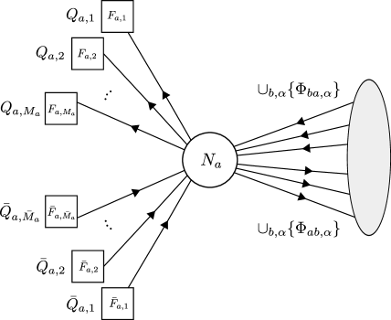
Figure 1: Representation of the arrows (fields) and square nodes (flavour symmetries) for a single gauge node labelled $a$. The shaded area represent the rest of the quiver.

In the generating function $\mathcal{Z}$, the chemical potential of a generic bi-fundamental field $\Phi_{ab,\alpha}$ will be denoted by $x_{ab,\alpha}$, while to each quark $Q_{a,\beta}$ and antiquark $\bar{Q}_{a,\gamma}$ we will assign the chemical potential matrices $\mathcal{T}_{a,\beta}$ and $\bar{\mathcal{T}}_{a,\gamma}$ respectively, defined as

$$\mathcal{T}_{a,\beta}=\text{diag}(t_{a,\beta,1},t_{a,\beta,2},...,t_{a,\beta,F_{a,\beta}})\,,\qquad\bar{\mathcal{T}}_{a,\gamma}=\text{diag}(\bar{t}_{a,\gamma,1},\bar{t}_{a,\gamma,2},...,\bar{t}_{a,\gamma,\bar{F}_{a,\gamma}})\,.$$ (2.1)

The entries of these matrices encode all of the quark and antiquark chemical potentials: $t_{a,\beta,k}=e^{i\theta_{a,\beta,k}}$ is the chemical potential for a quark $Q_{a,\beta,k}$ charged under the $U(1)_{k}$ of the maximal torus $\prod_{j=1}^{F_{a,\beta}}U(1)_{j}\subset U(F_{a,\beta})$, while $\bar{t}_{a,\gamma,k}=e^{-i\theta_{a,\gamma,k}}$ is the chemical potential for an antiquark $\bar{Q}_{a,\gamma,k}$ charged under the $U(1)_{k}$ of $\prod_{j=1}^{\bar{F}_{a,\gamma}}U(1)_{j}\subset U(\bar{F}_{a,\gamma})$.

	$U(N_{a})$	$U(N_{b})$	$U(F_{a,\beta})$	$U(\bar{F}_{a,\gamma})$
$\Phi_{ab,\alpha}$	$\bar{\Box}$	$\Box$	1	1
$\Phi_{aa,\alpha}$	Adj	1	1	1
$Q_{a,\beta}$	$\bar{\Box}$	1	$\Box$	1
$\bar{Q}_{a,\gamma}$	$\Box$	1	1	$\bar{\Box}$

Table 1: Gauge and flavour groups representations carried by $\Phi_{ab,\alpha}$, $Q_{a,\beta}$ and $\bar{Q}_{a,\gamma}$. $\Box$, $\bar{\Box}$ and 1 are respectively the fundamental, antifundamental and trivial representations of the correspondent group.

2.1 From gauge invariants to determinants and word counting

For quiver gauge theories with bi-fundamental fields, the generating function $\mathcal{Z}(\{x_{ab}\})$ for local holomorphic gauge invariant operators constructed from the chiral fields, is given by [1]

$$\mathcal{Z}(\{x_{ab,\alpha}\})=\prod_{i=1}F_{0}^{[n]}(\{x_{ab}\rightarrow\sum_{\alpha}x_{ab;\alpha}^{i}\})\,.$$ (2.2)

It is useful to introduce the complete $n$-node quiver which is a quiver that has $1$ edge for every specified start and end-point. An expression for $F_{0}^{[n]}(\{x_{ab}\})$ was given as the inverse of a sum over permutations of subsets of the set of nodes of the $n$-node complete quiver. Equivalently this is an expression in terms of loops in the complete quiver

$$F_{0}^{[n]}(\{y_{i}\})=\left(1+\sum_{\mathbb{V}\subseteq V_{n}}\,\sum_{\sigma\in\text{Symm}(\mathbb{V})}\,\prod_{i\in\text{Cycles}(\sigma)}\,\left(-y_{i}\right)\right)^{-1}\,.$$ (2.3)

Here $\mathbb{V}$ is any subset of nodes of the quiver (except the empty set), and for the cycle $(abc\cdots d)$ $y_{(abc\cdots d)}=x_{ab}x_{bc}\cdots x_{da}$. In this we observe, using standard matrix identities, that

$$F_{0}^{[n]}={1\over\det(\mathbb{1}_{n}-X_{n})}\,,$$ (2.4)

where $X_{n}$ is an $n\times n$ matrix with entries $x_{ab}$. This formula is the subject of the Mac Mahon master theorem [32].

While the function $\mathcal{Z}(\{x_{ab,\alpha}\})$ counts gauge invariant operators, the gauge theory set-up does not immediately offer a combinatoric interpretation for $F_{0}^{[n]}(\{x_{ab}\})$. We give an interpretation of $F_{0}^{[n]}$ in terms of word-counting problems associated with the complete $n$-node quiver. There are in fact two counting problems, one of them is a closed string counting problem. Consider a language where the words are made from letters which correspond to simple loops in the $n$-node quiver. These are loops that visit each node of the quiver no more than once. These letters equivalently correspond to cyclic permutations of any subset of integers $\{1,\cdots,n\}$. The words are constructed as strings, i.e. ordered sequences, of these letters with the additional equivalences introduced that letters corresponding to two simple loops $c$ and $c^{\prime}$ commute if the loops do not share a node. We denote these letters by $\hat{y}_{c}$. Then

$$\hat{y}_{c}\hat{y}_{c^{\prime}}=\hat{y}_{c^{\prime}}\hat{y}_{c}\,,$$ (2.5)

if $c$ and $c^{\prime}$ are loops that do not share a node. Any word contains a list of these letters $\hat{y}_{c_{1}},\hat{y}_{c_{2}}\cdots\hat{y}_{c_{k}}$ with multiplicities $(m_{1},m_{2},\cdots,m_{k})$. With these specified numbers, there is a multiplicity $\mathcal{M}(m_{1},\cdots,m_{k})$, of words since, in general, the order of the letters matters: if two loops $\hat{y}_{c},\hat{y}_{c^{\prime}}$ do share a node then $\hat{y}_{c}\hat{y}_{c^{\prime}}\neq\hat{y}_{c^{\prime}}\hat{y}_{c}$. The expansion of $F_{0}^{[n]}$ in terms of the loop variables contains terms of the form $y_{c_{1}}^{m_{1}}y_{c_{2}}^{m_{2}}\cdots y_{c_{k}}^{m_{k}}$ with coefficients, which are precisely the multiplicities of the words $\mathcal{M}(m_{1},\cdots,m_{k})$.

This is a remarkable new connection between a counting problem of words built from a partially commuting set of letters and the counting of gauge invariants. Since the letters correspond to simple loops, we call this the closed string word counting problem. Thus $F_{0}^{[n]}(\{x_{ab}\})$ generates multiplicities of closed string words. In section 4.3 we explain why this is true. Along the way, we introduce another word counting formula based on letters corresponding to open string bits.

2.2 Generalization to flavoured quivers

We extend the counting results to quivers that have bifundemental matter fields, as well as fundamental matter. We find again that the counting in the limit of large rank gauge groups is given as an infinite product. Each factor is obtained by making a simple substitution in a basic function $F^{[n]}(\{x_{ab},t_{a},\bar{t}_{a}\})$, for the case quivers with $n$ gauge nodes. The function $F^{[n]}$ has an elegant expression in terms of matrices $X_{n}$ and $\Lambda_{n}$, whose matrix elements are

$$\left.X_{n}\right|_{ab}=x_{ab}\,,\qquad\qquad\left.\Lambda_{n}\right|_{ab}=t_{a}\bar{t}_{b}\,.$$ (2.6)

Le us also define another $n\times n$ matrix,

$$\chi_{n}\equiv(\mathbb{1}_{n}-X_{n})^{-1}\,.$$ (2.7)

In terms of these, $F^{[n]}$ is the determinant

$$F^{[n]}(\{x_{ab}\},\{t_{a}\},\{\bar{t}_{a}\})=\det\left(\chi_{n}\,\exp\left[\chi_{n}\,\Lambda_{n}\right]\right)=\det(\chi_{n})\exp\left({\rm tr}\left(\chi_{n}\Lambda_{n}\right)\right)\,.$$ (2.8)

The generating function $\mathcal{Z}$ can be obtained through the infinite product

$${\mathcal{Z}}( \{x_{ab,\alpha}\},\{\mathcal{T}_{a,\beta}\},\{\bar{\mathcal{T}}_{a,\gamma}\})$$

$$=\prod_{i}F^{[n]}\left(\left\{x_{ab}\rightarrow\sum_{\alpha}x_{ab,\alpha}^{i}\right\},\left\{t_{a}\rightarrow\sum_{\beta}\frac{\text{Tr}(\mathcal{T}_{a,\beta}^{\,i})}{\sqrt{i}}\right\},\left\{\bar{t}_{a}\rightarrow\sum_{\gamma}\frac{\text{Tr}(\bar{\mathcal{T}}_{a,\gamma}^{\,i})}{\sqrt{i}}\right\}\right)\,\,.$$ (2.9)

In the course of our derivation of $F^{[n]}$, we find the identity

$$F^{[n]} =\det\left(\chi_{n}\,\exp\left[\chi_{n}\,\Lambda_{n}\right]\right)$$

$$=\sum_{\vec{p}\,}\,\prod_{a=1}^{n}\left(p_{a}+\sum_{b=1}^{n}p_{ab}\right)!\left(\prod_{b=1}^{n}\frac{x_{ab}^{\,p_{ab}}}{p_{ab}!}\right)\left(\frac{y_{a}^{\,p_{a}}}{p_{a}!}\right)\left(\frac{\bar{y}_{a}^{\,\bar{p}_{a}}}{\bar{p}_{a}!}\right)\,\delta\left(p_{a}-\bar{p}_{a}+\sum_{b=1}^{n}(p_{ab}-p_{ba})\right)\,,$$ (2.10)

with $\vec{p}=\bigcup_{a=1}^{n}\{\cup_{b=1}^{n}p_{ab},y_{a}^{p_{a}},\bar{y}_{a}^{\,\bar{p}_{a}}\}$. For the unflavoured case, this implies

$$F^{[n]}_{0} =\frac{1}{\det(\mathbb{1}_{n}-X_{n})}=\sum_{\vec{p}\,}\,\prod_{a=1}^{n}\left(\sum_{b=1}^{n}p_{ab}\right)!\left(\prod_{b=1}^{n}\frac{x_{ab}^{\,p_{ab}}}{p_{ab}!}\right)\delta\left(\sum_{b=1}^{n}(p_{ab}-p_{ba})\right)\,,$$ (2.11)

where now $\vec{p}=\bigcup_{a,b=1}^{n}\{p_{ab}\}$. This formula is interpreted in section 4.3 in terms of the counting of words built from partially commuting open string bits. The open string word counting has previously been studied in [23] and its equivalence to the closed string word counting given.

3 Group integral formula to partition sums

In this section we will derive a contour integral formulation for the generating function $\mathcal{Z}$. Our starting point is the group integral representation [25, 26]

$$\mathcal{Z}(\{x_{ab,\alpha}\}, \{t_{a,\beta,k}\},\{\bar{t}_{a,\gamma,k}\})=\int\left(\prod_{a}d\,U_{a}\right)$$

$$\times\prod_{a}\,\exp\left\{\sum_{i=1}^{\infty}\frac{1}{i}\left[\sum_{b,\alpha}x_{ab,\alpha}^{i}\,\text{Tr}(U_{a}^{\dagger i})\,\text{Tr}(U_{b}^{i})\right.\right.$$

$$\qquad\qquad\qquad\qquad\left.\left.+\sum_{\beta}\,\sum_{k=1}^{F_{a,\beta}}t_{a,\beta,k}^{i}\,\text{Tr}(U_{a}^{\dagger i})+\sum_{\gamma}\,\sum_{k=1}^{\bar{F}_{a,\gamma}}\bar{t}_{a,\gamma,k}^{i}\,\text{Tr}(U_{a}^{i})\right]\right\}\,.$$ (3.1)

Here $x_{ab,\alpha}$ is the chemical potential for the $\Phi_{ab,\alpha}$ field, while $t_{a,\beta,k}=e^{i\theta_{a,\beta,k}}$ is the chemical potential for a quark $Q_{a,\beta,k}$ charged under the $U(1)_{k}$ of the maximal torus $\prod_{j=1}^{F_{a,\beta}}U(1)_{j}\subset U(F_{a,\beta})$. Analogously, $\bar{t}_{a,\gamma,k}=e^{-i\theta_{a,\gamma,k}}$ is the chemical potential for an antiquark $\bar{Q}_{a,\gamma,k}$ charged under the $U(1)_{k}$ of $\prod_{j=1}^{\bar{F}_{a,\gamma}}U(1)_{j}\subset U(\bar{F}_{a,\gamma})$. Expanding the generating function gives the counting function $\mathcal{N}(\{n_{ab,\alpha}\},\{n_{a,\beta,k}\},\{\bar{n}_{a,\gamma,k}\})$ for specified numbers $n_{ab,\alpha}$ of bifundamentals $\Phi_{ab,\alpha}$, $n_{a,\beta,k}$ of quarks $Q_{a,\beta,k}$ and $\bar{n}_{a,\gamma,k}$ anti-quarks $\bar{Q}_{a,\gamma,k}$:

$$\mathcal{Z}(\{x_{ab,\alpha}\},\{t_{a,\beta,k}\},\{\bar{t}_{a,\gamma,k}\}) =\sum_{\{n_{ab,\alpha}\}}\,\sum_{\{n_{a,\beta,k}\}}\,\sum_{\{\bar{n}_{a,\gamma,k}\}}\,\mathcal{N}(\{n_{ab,\alpha}\},\{n_{a,\beta,k}\},\{\bar{n}_{a,\gamma,k}\})$$

$$\qquad\quad\times\left(\prod_{a,b,\alpha}\,x_{ab,\alpha}^{n_{ab,\alpha}}\right)\,\left(\prod_{a,\beta,k}\,t_{a,\beta,k}^{n_{a.\beta,k}}\right)\,\left(\prod_{a,\gamma,k}\,\bar{t}_{a,\gamma,k}^{\,\,\bar{n}_{a,\gamma,k}}\right)\,.$$ (3.2)

The chemical potentials for the quark/antiquark matter content can be nicely encoded in the unitary matrices $\mathcal{T}_{a,\beta}=\text{diag}(t_{a,\beta,1},t_{a,\beta,2},...,t_{a,\beta,F_{a,\beta}})$ and $\bar{\mathcal{T}}_{a,\gamma}=\text{diag}(\bar{t}_{a,\gamma,1},\bar{t}_{a,\gamma,2},...,\bar{t}_{a,\gamma,\bar{F}_{a,\gamma}})$ respectively, so that

$$\mathcal{Z}(\{x_{ab,\alpha}\}, \{\mathcal{T}_{a,\beta}\},\{\bar{\mathcal{T}}_{a,\gamma}\})=\int\left(\prod_{a}d\,U_{a}\right)\,\prod_{a}\,\exp\left\{\sum_{i=1}^{\infty}\frac{1}{i}\left[\sum_{b,\alpha}x_{ab,\alpha}^{i}\,\text{Tr}(U_{a}^{\dagger i})\,\text{Tr}(U_{b}^{i})\right.\right.$$

$$\qquad\qquad\qquad\qquad\left.\left.+\sum_{\beta}\,\text{Tr}(U_{a}^{\dagger i})\,\text{Tr}(\mathcal{T}_{a,\beta}^{i})+\sum_{\gamma}\,\text{Tr}(\bar{\mathcal{T}}_{a,\gamma}^{i})\,\text{Tr}(U_{a}^{i})\right]\right\}\,.$$ (3.3)

Using the shorthand notation $\int\left(\prod_{a}d\,U_{a}\right)\equiv\int$ and expanding the exponential function we get

$$\mathcal{Z}(\{ x_{ab,\alpha}\},\{\mathcal{T}_{a,\beta}\},\{\bar{\mathcal{T}}_{a,\gamma}\})$$

$$=\int\prod_{a}\left\{\left(\sum_{\{p_{ab,\alpha}^{(i)}\}_{a}}\,\prod_{b,\alpha}\,\frac{x_{ab,\alpha}^{\sum_{i}ip_{ab,\alpha}^{(i)}}}{\prod_{i}p_{ab,\alpha}^{(i)}!\,n^{p_{ab,\alpha}^{(i)}}}\,\prod_{i}\,(\text{Tr}\,U_{a}^{\dagger i})^{p_{ab,\alpha}^{(i)}}\,(\text{Tr}\,U_{b}^{i})^{p_{ab,\alpha}^{(i)}}\right)\right.$$ (3.4)

$$\qquad\qquad\qquad\qquad\times\left(\sum_{\{p_{a,\beta}^{(i)}\}_{a}}\,\prod_{\beta}\,\frac{1}{\prod_{i}p_{a,\beta}^{(i)}!\,n^{p_{a,\beta}^{(i)}}}\,\prod_{i}\,(\text{Tr}\,U_{a}^{\dagger i})^{p_{a,\beta}^{(i)}}\,(\text{Tr}\,\mathcal{T}_{a,\beta}^{i})^{p_{a,\beta}^{(i)}}\right)$$

$$\qquad\qquad\qquad\qquad\qquad\qquad\times\left.\left(\sum_{\{\bar{p}_{a,\gamma}^{(i)}\}_{a}}\,\prod_{\gamma}\,\frac{1}{\prod_{i}\bar{p}_{a,\gamma}^{(i)}!\,n^{\bar{p}_{a,\gamma}^{(i)}}}\,\prod_{i}\,(\text{Tr}\,\bar{\mathcal{T}}_{a,\gamma}^{i})^{\bar{p}_{a,\gamma}^{(i)}}\,(\text{Tr}\,U_{a}^{i})^{\bar{p}_{a,\gamma}^{(i)}}\right)\right\}\,,$$

where $\sum_{\{p_{ab,\alpha}^{(i)}\}_{a}}\equiv\prod_{i,b,\alpha}\,\sum_{p_{ab,\alpha}^{(i)}=0}^{\infty}$, $\sum_{\{p_{a,\beta}^{(i)}\}_{a}}\equiv\prod_{\beta,i}\sum_{p_{a,\beta,i}}$ and $\sum_{\{\bar{p}_{a,\gamma}^{(i)}\}_{a}}\equiv\prod_{\gamma,i}\sum_{p_{\gamma,i}}$. Rearranging sums and collecting like terms, we obtain

$$\mathcal{Z} (\{x_{ab,\alpha}\},\{\mathcal{T}_{a,\beta}\},\{\bar{\mathcal{T}}_{a,\gamma}\})$$

$$=\sum_{\{p_{ab,\alpha}^{(i)}\}}\,\sum_{\{p_{a,\beta}^{(i)}\}}\,\sum_{\{\bar{p}_{a,\gamma}^{(i)}\}}\,\int\left(\prod_{a,b,\alpha}\,\frac{x_{ab,\alpha}^{\sum_{i}ip_{ab,\alpha}^{(i)}}}{\prod_{i}p_{ab,\alpha}^{(i)}!\,n^{p_{ab,\alpha}^{(i)}}}\right)\,\left(\prod_{a,\beta}\,\frac{1}{\prod_{i}p_{a,\beta}^{(i)}!\,i^{p_{a,\beta}^{(i)}}}\right)\,\left(\prod_{a,\gamma}\,\frac{1}{\prod_{i}\bar{p}_{a,\gamma}^{(i)}!\,i^{\bar{p}_{a,\gamma}^{(i)}}}\right)$$

$$\qquad\times\left\{\prod_{a,i}\,(\text{Tr}\,U_{a}^{\dagger i})^{\sum_{b,\alpha}p_{ab,\alpha}^{(i)}+\sum_{\beta}p_{a,\beta}^{(i)}}\,\,(\text{Tr}\,U_{a}^{i})^{\sum_{b,\alpha}p_{ba,\alpha}^{(i)}+\sum_{\gamma}\bar{p}_{a,\gamma}^{(i)}}\right\}$$ (3.5)

$$\qquad\qquad\qquad\times\prod_{a,i}\,\left[\prod_{\beta}(\text{Tr}\,\mathcal{T}_{a,\beta}^{i})^{p_{a,\beta}^{(i)}}\right]\,\left[\prod_{\gamma}(\text{Tr}\,\bar{\mathcal{T}}_{a,\gamma}^{i})^{\bar{p}_{a,\gamma}^{(i)}}\right]\,.$$

We now collect powers of $x_{ab,\alpha},\mathcal{T}_{a,\beta},\bar{\mathcal{T}}_{a,\gamma}$ denoted $n_{ab,\alpha},n_{a,\beta},\bar{n}_{a,\gamma}$, and introduce the quantities

$$\vec{p}_{ab,\alpha}=\cup_{i}\{p_{ab,\alpha}^{(i)}\},\,\qquad\qquad\allowbreak\vec{p}_{a,\beta}=\cup_{i}\{p_{a,\beta}^{(i)}\},\,\qquad\qquad\vec{\bar{p}}_{a,\gamma}=\cup_{i}\{\bar{p}_{a,\gamma}^{\,(i)}\}\,.$$ (3.6)

These form partitions of $n_{ab,\alpha},\,n_{a,\beta},\,\bar{n}_{a,\gamma}$, which can be interpreted as cycle lengths of permutations $\sigma_{ab,\alpha}\in S_{n_{ab,\alpha}},\,\sigma_{a,\beta}\in S_{n_{a,\beta}}$ and $\bar{\sigma}_{a,\gamma}\in S_{\bar{n}_{a,\gamma}}$ respectively. These cycle structures determine conjugacy classes denoted $[\sigma_{ab,\alpha}],[\sigma_{a,\beta}],[\bar{\sigma}_{a,\gamma}]$. We have

$$\sum_{i=1}^{\infty}ip_{ab,\alpha}^{(i)}=n_{ab,\alpha}\,,\qquad\quad|\vec{p}_{ab,\alpha}|=\frac{n_{ab,\alpha}!}{\prod_{i}p_{ab,\alpha}^{(i)}!\,i^{p_{ab,\alpha}^{(i)}}}\,,$$ (3.7)

and similarly for $\vec{p}_{a,\beta}$ and $\vec{\bar{p}}_{a,\gamma}$. The second equation above gives the number of permutations with the specified cycle structure. We also use the identity

$$\prod_{i}\,(\text{Tr}\,U^{i})^{[\sigma]^{(i)}}=\sum_{R\vdash n\atop l(R)\leq N}\chi_{R}(\sigma)\chi_{R}(U)\,,\qquad\sigma\in S_{n}\,,\,\,\,U\in U(N)\,,$$ (3.8)

which follows from Schur-Weyl duality (see e.g. [27]): here $R$ is a partition of $n$ and $[\sigma]^{(i)}$ is the number of cycles of length $i$ in $\sigma$, which is a function of the conjugacy class $[\sigma]$. The Young diagrams are constrained to have no more than $N$ rows, which is expressed as $l(R)\leq N$. This encodes the constraints following from finiteness of the ranks $N_{a}$. For $n_{a}\leq N_{a}$, these constraints can be dropped, which is the origin of simplifications at large $N_{a}$. Collecting powers of traces of $U_{a}^{\dagger}$, this equation can be used to rewrite the traces in (3) as

$$\prod_{i} \,(\text{Tr}\,U_{a}^{\dagger i})^{\sum_{b,\alpha}p_{ab,\alpha}^{(i)}+\sum_{\beta}p_{a,\beta}^{(i)}}=\sum_{R_{a}\vdash n_{a}\atop l(R_{a})\leq N_{a}}\chi_{R_{a}}(\times_{b,\alpha}\sigma_{ab,\alpha}\times_{\beta}\sigma_{a,\beta})\chi_{R_{a}}(U_{a}^{\dagger})\,,$$

$$\qquad\qquad\quad n_{a}=\sum_{b,\alpha}n_{ab,\alpha}+\sum_{\beta}n_{a,\beta}\,,$$ (3.9)

and similarly for the other terms. The product of the permutations over $b,\,\alpha,\,\beta$ describes an outer product of permutations acting on subsets of size $n_{ab,\alpha},\,n_{a,\beta}$ of $n_{a}$. Using these definitions, we can write

$$\mathcal{Z} (\{x_{ab,\alpha}\},\{\mathcal{T}_{a,\beta}\},\{\bar{\mathcal{T}}_{a,\gamma}\})=\sum_{\{n_{ab,\alpha}\}}\,\sum_{\{n_{a,\beta}\}\atop\{\bar{n}_{a,\gamma}\}}\sum_{\{\vec{p}_{ab,\alpha}\}}\,\sum_{\{\vec{p}_{a,\beta}\}}\,\sum_{\{\vec{\bar{p}}_{a,\gamma}\}}$$ (3.10)

$$\times\int\left(\prod_{a,b,\alpha}\,\frac{x_{ab,\alpha}^{n_{ab,\alpha}}}{n_{ab,\alpha}!}\,|\vec{p}_{ab,\alpha}|\right)\,\left(\prod_{a,\beta}\,\frac{1}{n_{a,\beta}!}\,|\vec{p}_{a,\beta}|\right)\,\left(\prod_{a,\gamma}\,\frac{1}{\bar{n}_{a,\gamma}!}\,|\vec{\bar{p}}_{a,\gamma}|\right)$$

$$\times\prod_{a}\,\left\{\sum_{R_{a}\vdash n_{a}\atop l(R_{a})\leq N_{a}}\sum_{S_{a}\vdash n_{a}\atop l(S_{a})\leq N_{a}}\chi_{R_{a}}(\times_{b,\alpha}\sigma_{ab,\alpha}\times_{\beta}\sigma_{a,\beta})\,\chi_{S_{a}}(\times_{b,\alpha}\sigma_{ba,\alpha}\times_{\gamma}{\bar{\sigma}}_{a,\gamma})\,\chi_{R_{a}}(U_{a}^{\dagger})\,\chi_{S_{a}}(U_{a})\right\}$$

$$\times\prod_{a}\,\left\{\sum_{\left\{r_{a,\beta}\vdash n_{a,\beta}\atop l(r_{a,\beta})\leq F_{a,\beta}\right\}_{a}}\,\prod_{\beta}\chi_{r_{a,\beta}}(\sigma_{a,\beta})\chi_{r_{a,\beta}}(\mathcal{T}_{a,\beta})\right\}\left\{\sum_{\left\{\bar{r}_{a,\gamma}\vdash\bar{n}_{a,\gamma}\atop l(\bar{r}_{a,\gamma})\leq\bar{F}_{a,\gamma}\right\}_{a}}\,\prod_{\gamma}\chi_{\bar{r}_{a,\gamma}}({\bar{\sigma}}_{a,\gamma})\chi_{\bar{r}_{a,\gamma}}(\bar{\mathcal{T}}_{a,\gamma})\right\}\,,$$

where $\sigma_{ab,\alpha}$, $\sigma_{a,\beta}$ and $\bar{\sigma}_{a,\gamma}$ are representatives of the conjugacy classes specified by $\vec{p}_{ab,\alpha}$, $\vec{p}_{a,\beta}$ and $\vec{\bar{p}}_{a,\gamma}$ respectively. We can now cast the sums over these vectors into sums over the permutations $\sigma_{ab,\alpha}\in S_{n_{ab,\alpha}}$, $\sigma_{a,\beta}\in S_{n_{a,\beta}}$ and $\bar{\sigma}_{a,\gamma}\in S_{\bar{n}_{a,\gamma}}$. We also use the symmetric group character expansion

$$\chi_{R_{a}} (\times_{b,\alpha}\sigma_{ab,\alpha}\times_{\beta}\sigma_{a,\beta})$$

$$=\sum_{\cup_{b,\alpha}\{r_{ab,\alpha}\vdash n_{ab,\alpha}\}\atop\cup_{\beta}\{r_{a,\beta}\vdash n_{a,\beta}\}}g(\cup_{b,\alpha}r_{ab,\alpha}\cup_{\beta}r_{a,\beta};R_{a})\left(\prod_{b,\alpha}\,\chi_{r_{ab,\alpha}}(\sigma_{ab,\alpha})\right)\,\left(\prod_{\beta}\,\chi_{r_{,\beta}}(\sigma_{a,\beta})\right)\,,$$ (3.11)

and similarly for $\chi_{S_{a}}(\times_{b,\alpha}\sigma_{ba,\alpha}\times_{\gamma}{\bar{\sigma}}_{a,\gamma})$. In the formula above, $g(\cup_{b,\alpha}r_{ab,\alpha}\cup_{\beta}r_{a,\beta};R_{a})$ is a Littlewood-Richardson coefficient. This is the multiplicity of the representation $\otimes_{b,\alpha}r_{a,b,\alpha}\otimes_{\beta}r_{a,\beta}$ of the subgroup $\times_{b,\alpha}S_{n_{ab,\alpha}}\times_{\beta}S_{n_{a,\beta}}$ when the representation $R_{a}$ of $S_{n_{a}}$ is decomposed into irreducibles of the product subgroup. Finally, using use the $U(N)$ character orthogonality formula

$$\int d\,U\,\chi_{R}(U^{\dagger})\chi_{S}(U)=\delta_{R,S}\,.$$ (3.12)

we obtain

$$\mathcal{Z} (\{x_{ab,\alpha}\},\{\mathcal{T}_{a,\beta}\},\{\bar{\mathcal{T}}_{a,\gamma}\})$$

$$=\sum_{\{n_{ab,\alpha}\}}\,\sum_{\{n_{a,\beta}\}\atop\{\bar{n}_{a,\gamma}\}}\,\sum_{\{\sigma_{ab,\alpha}\}}\,\sum_{\{\sigma_{a,\beta}\}}\,\sum_{\{\bar{\sigma}_{a,\gamma}\}}\left(\prod_{a,b,\alpha}\,\frac{x_{ab,\alpha}^{n_{ab,\alpha}}}{n_{ab,\alpha}!}\,\right)\,\left(\prod_{a,\beta}\,\frac{1}{n_{a,\beta}!}\right)\,\left(\prod_{a,\gamma}\,\frac{1}{\bar{n}_{a,\gamma}!}\right)$$

$$\,\times\sum_{\left\{R_{a}\vdash n_{a}\atop l(R_{a})\leq N_{a}\right\}}\sum_{\{r_{ab,\alpha}\vdash n_{ab,\alpha}\}\atop\{s_{ab,\alpha}\vdash n_{ab,\alpha}\}}\,\sum_{\{s_{a,\beta}\vdash n_{a,\beta}\}\atop\{\bar{s}_{a,\gamma}\vdash\bar{n}_{a,\gamma}\}}\,\left\{\prod_{a}g(\cup_{b,\alpha}r_{ab,\alpha}\cup_{\beta}s_{a,\beta};R_{a})\,g(\cup_{b,\alpha}s_{ba,\alpha}\cup_{\gamma}\bar{s}_{a,\gamma};R_{a})\right\}$$

$$\qquad\times\left(\prod_{a,b,\alpha}\,\chi_{r_{ab,\alpha}}(\sigma_{ab,\alpha})\chi_{s_{ba,\alpha}}(\sigma_{ba,\alpha})\right)\,\left(\prod_{a,\beta}\,\chi_{s_{a,\beta}}(\sigma_{a,\beta})\right)\,\left(\prod_{a,\gamma}\,\chi_{\bar{s}_{,\gamma}}(\bar{\sigma}_{a,\gamma})\right)$$

$$\qquad\times\sum_{\{r_{a,\beta}\vdash n_{a,\beta}\}\atop\{\bar{r}_{a,\gamma}\vdash\bar{n}_{a,\gamma}\}}\left\{\prod_{a,\beta}\chi_{r_{a,\beta}}(\sigma_{a,\beta})\chi_{r_{a,\beta}}(\mathcal{T}_{a,\beta})\right\}\left\{\prod_{a,\gamma}\chi_{\bar{r}_{a,\gamma}}({\bar{\sigma}}_{a,\gamma})\chi_{\bar{r}_{a,\gamma}}(\bar{\mathcal{T}}_{a,\gamma})\right\}\,.$$ (3.13)

Note that we dropped the $l(r_{a,\beta})\leq F_{a,\beta}$ constraint on the sum over quark representations, since contributions coming from representations with $l(r_{a,\beta})>F_{a,\beta}$ are automatically zero due to the vanishing of $\chi_{r_{a,\beta}}(\mathcal{T}_{a,\beta})$ (similar comments hold for the sum over antiquark representations as well).

Finally, using the orthogonality of the symmetric group characters $\sum_{\sigma\in S_{n}}\chi_{r}(\sigma)\chi_{s}(\sigma)=n!\delta_{r,s}$, we get the formula

$$\mathcal{Z} (\{x_{ab,\alpha}\},\{\mathcal{T}_{a,\beta}\},\{\bar{\mathcal{T}}_{a,\gamma}\})=\sum_{\{n_{ab,\alpha}\}}\,\sum_{\{n_{a,\beta}\}\atop\{\bar{n}_{a,\gamma}\}}\,\left(\prod_{a,b,\alpha}\,x_{ab,\alpha}^{n_{ab,\alpha}}\right)\,\sum_{\left\{R_{a}\vdash n_{a}\atop l(R_{a})\leq N_{a}\right\}}\,\sum_{\{r_{ab,\alpha}\vdash n_{ab,\alpha}\}}\,\sum_{\{r_{a,\beta}\vdash n_{a,\beta}\}\atop\{\bar{r}_{a,\gamma}\vdash\bar{n}_{a,\gamma}\}}$$ (3.14)

$$\prod_{a}\,g(\cup_{b,\alpha}r_{ab,\alpha}\cup_{\beta}r_{a,\beta};R_{a})\,g(\cup_{b,\alpha}r_{ba,\alpha}\cup_{\gamma}\bar{r}_{a,\gamma};R_{a})\ \left(\prod_{\beta}\chi_{r_{a,\beta}}(\mathcal{T}_{a,\beta})\right)\left(\prod_{\gamma}\chi_{\bar{r}_{a,\gamma}}(\bar{\mathcal{T}}_{a,\gamma})\right)\,.$$

Note that setting $\mathcal{T}_{a,\beta}=t_{a,\beta}\,\mathbb{1}_{a,\beta}$ ($\bar{\mathcal{T}}_{a,\gamma}=\bar{t}_{a,\gamma}\,\mathbb{1}_{a,\gamma}$) gives an unrefined generating function, in which we no longer distinguish quark (antiquark) states charged under different $U(1)$ factors in the maximal torus of $U(F_{a,\beta})$ ($U(\bar{F}_{a,\gamma})$). This unrefinement is immediately obtained from (3.14) through the substitutions

$$\chi_{r_{a,\beta}}(\mathcal{T}_{a,\beta})\rightarrow\text{dim}^{U(F_{a,\beta})}(r_{a,\beta})\,t_{a,\beta}^{n_{a,\beta}}\,,\qquad\quad\chi_{\bar{r}_{a,\gamma}}(\bar{\mathcal{T}}_{a,\gamma})\rightarrow\text{dim}^{U(\bar{F}_{a,\gamma})}(\bar{r}_{a,\gamma})\,\bar{t}_{a,\gamma}^{\,\bar{n}_{a,\gamma}}\,.$$ (3.15)

The $\text{dim}^{U(F)}(r)$ is the dimension of the representation $r$ of $U(F)$.

For an $F$ dimensional unitary matrix $\mathcal{T}$ with eigenvalues $(t_{1},t_{2},...,t_{F})$ and a partition $R$ of $n$, we have

$$\chi_{R}(\mathcal{T})=\sum_{\sigma\in S_{n}}\frac{\chi_{R}(\sigma)}{n!}\prod_{i}(\text{Tr}\,\mathcal{T}^{i})^{[\sigma]^{(i)}}=\sum_{\{n_{j}\}}g(\cup_{j}[n_{j}];R)\,\prod_{j=1}^{F}\,t_{j}^{n_{j}}\,,$$ (3.16)

where $n=\sum_{j}n_{j}$ and $[n_{j}]$ is the single-row totally symmetric representation of $S_{n_{j}}$. These Littlewood-Richardson multiplicities for single-row representations and a general $R$ are called Kostka numbers [27]. Note also that the Littlewood-Richardson multiplicities satisfy [27, 33]

$$\sum_{s}g(r_{1},s;R)g(r_{2},r_{3};s)=g(r_{1},r_{2},r_{3};R)\,.$$ (3.17)

Using these identities, we can write the counting function $\mathcal{N}(\{n_{ab,\alpha}\},\{n_{a,\beta,k}\},\{\bar{n}_{a,\gamma,k}\})$ as

$$\mathcal{N} (\{n_{ab,\alpha}\},\{n_{a,\beta,k}\},\{\bar{n}_{a,\gamma,k}\})$$ (3.18)

$$=\sum_{\left\{R_{a}\vdash n_{a}\atop l(R_{a})\leq N_{a}\right\}}\,\sum_{\{r_{ab,\alpha}\vdash n_{ab,\alpha}\}}\,\prod_{a}\,g(\cup_{b,\alpha}r_{ab,\alpha}\cup_{\beta,k}[n_{a,\beta,k}];R_{a})\,g(\cup_{b,\alpha}r_{ba,\alpha}\cup_{\gamma,k}[\bar{n}_{a,\gamma,k}];R_{a})\,,$$

where $n_{a}=\sum_{b,\alpha}n_{ab,\alpha}+\sum_{\beta,k}n_{a,\beta,k}$.

We can give a pictorial interpretation of the counting function (3.18) as follows.

• Choose the set of integers $\cup_{a,b,\alpha}\{n_{ab,\alpha}\}\cup_{a,\beta,k}\{n_{a,\beta,k}\}\cup_{a,\gamma,k}\{\bar{n}_{a,\gamma,k}\}$ These determine the numbers of elementary fields of various types in the composite operators under consideration.

• To all edges joining the gauge node $a$ to the gauge node $b$, associate a representation $r_{ab,\alpha}$ of the symmetric group $S_{n_{ab,\alpha}}$.

• Divide each gauge node $a$ into two components, $a^{+}$ and $a^{-}$: the former collects all the edges coming into the node $a$, while the latter collects all the edges leaving the node $a$. Connect $a^{+}$ to $a^{-}$ by adding a directed edge carrying a representation $R_{a}$ of $S_{n_{a}}$, where $n_{a}=\sum_{b,\alpha}n_{ab,\alpha}+\sum_{\beta,k}n_{a,\beta,k}$. The result is called split-node quiver.

• To each $a^{-}$ attach the Littlewood-Richardson coefficient $g(\cup_{b,\alpha}r_{ab,\alpha}\cup_{\beta,k}[n_{a,\beta,k}];R_{a})$; to each $a^{+}$ attach the Littlewood-Richardson coefficient $g(\cup_{b,\alpha}r_{ba,\alpha}\cup_{\gamma,k}[\bar{n}_{a,\gamma,k}];R_{a})$.

• Take the product of all the Littlewood-Richardson coefficients obtained in the previous step and sum over all possible representations $\{R_{a}\}$ and $\{r_{ab,\alpha}\}$, imposing finite $N$ constraints $l(R_{a})\leq N_{a}$ at each gauge node $a$.

As an example of the application of (3.14), consider an $\mathcal{N}=2$ SQCD with an adjoint hypermultiplet. The $\mathcal{N}=1$ quiver diagram for this gauge theory and its corresponding split node quiver are depicted in figure 2.

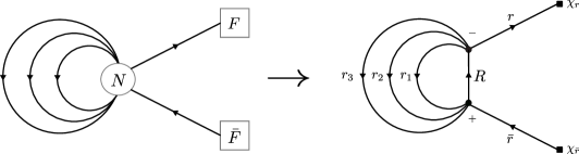
Figure 2: The $\mathcal{N}=1$ quiver and the corresponding split node diagram for a $\mathcal{N}=2$ SQCD with an adjoint hypermultiplet.

The generating function for this model can then be readily obtained using (3.14):

$$\mathcal{Z}(x_{1},x_{2},x_{3},\mathcal{T},\bar{\mathcal{T}}) =\sum_{n_{1},n_{2},n_{3}=0}^{\infty}\,\,\sum_{n,\bar{n}=0}^{\infty}\,x_{1}^{n_{1}}\,x_{2}^{n_{2}}\,x_{3}^{n_{3}}$$ (3.19)

$$\qquad\times\,\sum_{R\vdash m\atop l(R)\leq N}\,\sum_{{{r_{1}\vdash n_{1}}\atop r_{2}\vdash n_{2}}\atop r_{3}\vdash n_{3}}\,\sum_{r\vdash n\atop\bar{r}\vdash\bar{n}}g(r_{1},r_{2},r_{3},r;R)\,g(r_{1},r_{2},r_{3},\bar{r};R)\,\chi_{r}(\mathcal{T})\,\chi_{\bar{r}}(\bar{\mathcal{T}})\,,$$

with $m=n_{1}+n_{2}+n_{3}+n=n_{1}+n_{2}+n_{3}+\bar{n}$. On the other hand, using (3.18) we can write the counting function

$$\mathcal{N}( n_{1},n_{2},n_{3},\{n_{j}\},\{\bar{n}_{k}\})$$

$$=\sum_{R\vdash m\atop l(R)\leq N}\,\sum_{{{r_{1}\vdash n_{1}}\atop r_{2}\vdash n_{2}}\atop r_{3}\vdash n_{3}}\,g(r_{1},r_{2},r_{3},[n_{1}],[n_{2}],\cdots,[n_{F}];R)\,g(r_{1},r_{2},r_{3},[\bar{n}_{1}],[\bar{n}_{2}],\cdots,[\bar{n}_{\bar{F}}];R)\,,$$ (3.20)

so that

$$\mathcal{Z}\left(x_{1},x_{2},x_{3},\{t_{j}\},\{\bar{t}_{k}\}\right)=\sum_{n_{1},n_{2},n_{3}}\,\sum_{\{n_{j}\}}\,\sum_{\{\bar{n}_{k}\}} \,\,\mathcal{N}(n_{1},n_{2},n_{3},\{n_{j}\},\{\bar{n}_{k}\})$$

$$\times\,x_{1}^{n_{1}}\,x_{2}^{n_{2}}\,x_{3}^{n_{3}}\,\left(\prod_{j=1}^{F}t_{j}^{n_{j}}\right)\left(\prod_{k=1}^{\bar{F}}\bar{t}_{k}^{\,\,\bar{n}_{k}}\right)\,.$$ (3.21)

Let us now consider the flavoured conifold gauge theory [21, 22, 34, 35], whose quiver is depicted in figure 3:

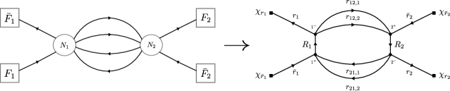
Figure 3: The flavoured conifold quiver and its split node quiver.

Applying (3.14), we find that the generating function for the flavoured conifold is

$$\mathcal{Z}(x_{12,1},x_{12,2},x_{21,1},x_{21,2},\mathcal{T}_{1},\mathcal{T}_{2},\bar{\mathcal{T}}_{1},\bar{\mathcal{T}}_{2})$$

$$=\sum_{n_{12,1},n_{12,2}=0}^{\infty}\,\,\sum_{n_{21,1},n_{21,2}=0}^{\infty}\,\,x_{12,1}^{n_{12,1}}\,x_{12,2}^{n_{12,2}}\,x_{21,1}^{n_{21,1}}\,x_{21,2}^{n_{21,2}}\,\sum_{R_{1}\vdash m_{1}\atop l(R_{1})\leq N_{1}}\,\sum_{R_{2}\vdash m_{2}\atop l(R_{2})\leq N_{2}}\,\sum_{r_{12,1}\vdash n_{12,1}\atop r_{12,2}\vdash n_{12,2}}\,\sum_{r_{21,1}\vdash n_{21,1}\atop r_{21,2}\vdash n_{21,2}}\,\sum_{r_{1}\vdash n_{1}\atop\bar{r}_{1}\vdash\bar{n}_{1}}\,\sum_{r_{2}\vdash n_{2}\atop\bar{r}_{2}\vdash\bar{n}_{2}}$$

$$\qquad\qquad\times g(r_{12,1},r_{12,2},r_{1};R_{1})\,g(r_{21,1},r_{21,2},\bar{r}_{1};R_{1})\,\chi_{r_{1}}(\mathcal{T}_{1})\,\chi_{\bar{r}_{1}}(\bar{\mathcal{T}}_{1})$$

$$\qquad\qquad\qquad\times g(r_{21,1},r_{21,2},r_{2};R_{2})\,g(r_{12,1},r_{12,2},\bar{r}_{2};R_{2})\,\chi_{r_{2}}(\mathcal{T}_{2})\,\chi_{\bar{r}_{2}}(\bar{\mathcal{T}}_{2})\,,$$ (3.22)

where $m_{1}=n_{12,1}+n_{12,2}+n_{1}=n_{21,1}+n_{21,2}+\bar{n}_{1}$ and $m_{2}=n_{21,1}+n_{21,2}+n_{2}=n_{12,1}+n_{12,2}+\bar{n}_{2}$. As in the previous example, using (3.18) we get

$$\mathcal{N} (n_{12,1},\,n_{12,2},\,n_{21,1},\,n_{21,2},\{n_{1,j}\},\{n_{2,j}\},\{\bar{n}_{1,k}\},\{\bar{n}_{2,k}\})=\sum_{R_{1}\vdash m_{1}\atop l(R_{1})\leq N_{1}}\,\sum_{R_{2}\vdash m_{2}\atop l(R_{2})\leq N_{2}}\,\sum_{r_{12,1}\vdash n_{12,1}\atop r_{12,2}\vdash n_{12,2}}\,\sum_{r_{21,1}\vdash n_{21,1}\atop r_{21,2}\vdash n_{21,2}}$$

$$\times\,g(r_{12,1},r_{12,2},[n_{1,1}],[n_{1,2}],\cdots,[n_{1,F_{1}}];R_{1})\,g(r_{21,1},r_{21,2},[\bar{n}_{1,1}],[\bar{n}_{1,2}],\cdots,[\bar{n}_{1,\bar{F}_{1}}];R_{1})$$

$$\quad\times g(r_{21,1},r_{21,2},[n_{2,1}],[n_{2,2}],\cdots,[n_{2,F_{2}}];R_{2})\,g(r_{12,1},r_{12,2},[\bar{n}_{2,1}],[\bar{n}_{2,2}],\cdots,[\bar{n}_{2,\bar{F}_{2}}];R_{2})\,,$$ (3.23)

so that

$$\mathcal{Z}( x_{12,1},\,x_{12,2},\,x_{21,1},\,x_{21,2},\{t_{1,j}\},\{t_{2,j}\},\{\bar{t}_{1,k}\},\{\bar{t}_{2,k}\})$$

$$=\sum_{n_{12,1}\atop n_{12,2}}\,\,\sum_{n_{21,1}\atop n_{21,2}}\,\sum_{\{n_{1,j}\}}\,\sum_{\{n_{2,j}\}}\,\sum_{\{\bar{n}_{1,k}\}}\,\sum_{\{\bar{n}_{2,k}\}}\,\mathcal{N}(n_{12,1},\,n_{12,2},\,n_{21,1},\,n_{21,2},\{n_{1,j}\},\{n_{2,j}\},\{\bar{n}_{1,k}\},\{\bar{n}_{2,k}\})$$

$$\qquad\qquad\times\,x_{12,1}^{n_{12,1}}\,x_{12,2}^{n_{12,2}}\,x_{21,1}^{n_{21,1}}\,x_{21,2}^{n_{21,2}}\,\left(\prod_{j=1}^{F_{1}}t_{1,j}^{n_{1,j}}\right)\,\left(\prod_{j=1}^{F_{2}}t_{2,j}^{n_{2,j}}\right)\,\left(\prod_{k=1}^{\bar{F}_{1}}\bar{t}_{1,k}^{\,\,\bar{n}_{1,k}}\right)\,\left(\prod_{k=1}^{\bar{F}_{2}}\bar{t}_{2,k}^{\,\,\bar{n}_{2,k}}\right)\,.$$ (3.24)

All of the previous formulae hold for any $N$. In the next section we will drop the $l(R_{a})\leq N_{a}$ constraints, $\forall a$, to focus on the large $N$ case.

3.1 The generating function $\mathcal{Z}$ and the building block $F^{[n]}$

Let us take the large $N$ limit, for all the gauge groups of the theory. In appendix A.1 we show that $\mathcal{Z}(\{x_{ab,\alpha}\},\{\mathcal{T}_{a,\beta}\},\{\bar{\mathcal{T}}_{a,\gamma}\})$ can be written as the multiple sum

$$\mathcal{Z}= \sum_{\boldsymbol{p}}\,\prod_{i}\,\prod_{a}\,\left(\prod_{b,\alpha}\frac{x_{ab,\alpha}^{n_{ab,\alpha}}}{p_{ab,\alpha}^{(i)}!}\right)\,\left(\prod_{\beta}\frac{(\text{Tr}\,\mathcal{T}_{a,\beta}\,^{i})^{\,p_{a,\beta}^{(i)}}}{p_{a,\beta}^{(i)}!}\right)\,\left(\prod_{\gamma}\frac{(\text{Tr}\,\bar{\mathcal{T}}_{a,\gamma}\,^{i})^{\,\bar{p}_{a,\gamma}^{(i)}}}{\bar{p}_{a,\gamma}^{(i)}!}\right)$$

$$\times\cfrac{\left(\sum_{b,\alpha}p_{ab,\alpha}^{(i)}+\sum_{\beta}p_{a,\beta}^{(i)}\right)!}{i^{\sum_{\beta}p_{a,\beta}^{(i)}}}\,\,\delta_{a}\left(\sum_{b,\alpha}(p_{ab,\alpha}^{(i)}-p_{ba,\alpha}^{(i)})+\sum_{\beta}p_{a,\beta}^{(i)}-\sum_{\gamma}\bar{p}_{a,\gamma}^{(i)}\right)\,,$$ (3.25)

where $\boldsymbol{p}=\cup_{ab,\alpha}\vec{p}_{ab,\alpha}\cup_{a,\beta}\vec{p}_{a,\beta}\cup_{a,\gamma}\vec{\bar{p}}_{a,\gamma}$, and the vectors $\vec{p}_{ab,\alpha},\,\vec{p}_{a,\beta},\,\vec{\bar{p}}_{a,\gamma}$ are defined in (3.6).

Crucially, we can now define the quantity

$$F^{[n]}(\{x_{ab}\},\{t_{a}\},\{\bar{t}_{a}\}\})= \sum_{\vec{p}}\prod_{a=1}^{n}\left(\sum_{b=1}^{n}p_{ba}+\bar{p}_{a}\right)!\,\,\delta_{a}\left(\sum_{b=1}^{n}(p_{ab}-p_{ba})+p_{a}-\bar{p}_{a}\right)$$

$$\qquad\qquad\times\left(\prod_{b=1}^{n}\frac{x_{ab}^{p_{ab}}}{p_{ab}!}\right)\,\left(\frac{t_{a}^{p_{a}}}{p_{a}!}\right)\,\left(\frac{\bar{t}_{a}^{\,\bar{p}_{a}}}{\bar{p}_{a}!}\right)\,,$$ (3.26)

with $\vec{p}=\cup_{a,b}\{p_{ab}\}\cup_{a}\{p_{a},\,\bar{p}_{a}\}$, such that

$${\mathcal{Z}}( \{x_{ab,\alpha}\},\{\mathcal{T}_{a,\beta}\},\{\bar{\mathcal{T}}_{a,\gamma}\})$$

$$=\prod_{i}F^{[n]}\left(\left\{x_{ab}\rightarrow\sum_{\alpha}x_{ab,\alpha}^{i}\right\},\left\{t_{a}\rightarrow\sum_{\beta}\frac{\text{Tr}(\mathcal{T}_{a,\beta}^{\,i})}{i}\right\},\left\{\bar{t}_{a}\rightarrow\sum_{\gamma}\text{Tr}(\bar{\mathcal{T}}_{a,\gamma}^{\,i})\right\}\right)\,\,.$$ (3.27)

From this equation we see that $F^{[n]}$ is the building block of $\mathcal{Z}$. Note that the $t$ coefficients in the RHS of (3.1) are weighted by a $i^{-1}$ coefficient, while the $\bar{t}$ coefficients are not: in section 5 we will derive a more symmetric version of this formula, where the weighting for chemical potentials of the quark and antiquark field is the same.

In appendix A.2 we derive an expression for $F^{[n]}$ in terms of contour integrals, namely

$$F^{[n]}(\{x_{ab}\},\{t_{a}\},\{\bar{t}_{a}\})=\left(\prod_{a=1}^{n}\oint_{\mathcal{C}_{a}}\frac{dz_{a}}{2\pi i}\right)\prod_{a=1}^{n}\,I_{a}(\vec{z};\vec{x}_{a},t_{a},\bar{t}_{a})\,,$$ (3.28)

in which

$$\vec{z}=(z_{1},z_{2},...,z_{n})\,,\qquad\vec{x}_{a}=(x_{1a},x_{2a},...,x_{na})\,,$$ (3.29)

and

$$I_{a}(\vec{z};\vec{x}_{a},t_{a},\bar{t}_{a})=\cfrac{\exp\left(z_{a}\,t_{a}\right)}{z_{a}-\left(\bar{t}_{a}+\sum_{b}z_{b}\,x_{ba}\right)}\,.$$ (3.30)

We also obtained a pole prescription for the computation of these contour integrals: in the appendices A and B we explain that only the $z_{a}$ pole coming from the $I_{a}$ term in the integrand has to be enclosed by $\mathcal{C}_{a}$.

As a last remark, note that all the variables $z_{a},\,x_{ab},\,t_{a},\,\bar{t}_{a}$ in eq. (3.28) are charged under the $\prod_{a=1}^{n}U(1)_{a}\subset\prod_{a=1}^{n}U(N_{a})$ subgroup of the theory as follows:

Variable	Charge	Subgroup of $\prod_{a}U(1)_{a}$
$x_{ab}$	$(-1,1)$	$U(1)_{a}\times U(1)_{b}$
$t_{a}$	$-1$	$U(1)_{a}$
$\bar{t}_{a}$	$1$	$U(1)_{a}$
$z_{a}$	$1$	$U(1)_{a}$

Table 2: $U(1)$ charges of the variables appearing in $F^{[n]}$.

The charge for the $x_{ab}$ coefficients comes from the fact that these variables are associated to fields leaving node $a$ and joining node $b$, thus transforming under $(\bar{N}_{a},N_{b})$ in the original theory. Similar comments holds for the charges of $t_{a}$ and $\bar{t}_{a}$, while the charge for $z_{a}$ has been chosen in such a way that the function $F^{[n]}$ is neutral under $\prod_{a}U(1)_{a}$, as it should be.

For completeness, let us write down the contour integral formulation for $\mathcal{Z}$, which can be immediately obtained from (3.1) by means of (3.1), and reads

$${\mathcal{Z}}= \prod_{i}\left(\prod_{a}\oint_{\mathcal{C}_{a,i}}\frac{dz_{a,i}}{2\pi iz_{a,i}}\right)\prod_{a}\,\cfrac{\exp\left(\cfrac{z_{a,i}\sum_{\beta}\text{Tr}(\mathcal{T}_{a,\beta}\,^{i})}{i}\right)}{1-z_{a,i}^{-1}\left(\sum_{\gamma}\text{Tr}(\bar{\mathcal{T}}_{a,\gamma}\,^{i})+\sum_{b,\alpha}z_{b,i}\,x_{ba,\alpha}^{i}\right)}\,.$$ (3.31)

The simplification coming from using $F^{[n]}$ in place of the latter is evident.

4 The unflavoured case: contour integrals and paths on graphs

We now have to calculate the contour integral in $F^{[n]}$, that is, calculate residues. In an $n$-node quiver, each $z_{a}$ variable has $n$ poles, but not all of them have to be included in the contour $\mathcal{C}_{a}$. The constraints from the convergence of the sums in appendix A.2.2 instruct us on which poles to pick and which ones to discard. In appendix B we show that they indeed give us a very simple and intuitive prescription: for all $a$, only the $z_{a}$ pole coming from the $I_{a}$ integrand has to be enclosed by $\mathcal{C}_{a}$.

We consider here the case in which we set $t_{a}=\bar{t}_{a}=0$ $\forall\,a$ in (3.28), to get the quantity

$$F^{[n]}(\{x_{ab}\},0,0)\equiv F_{0}^{[n]}(\{x_{ab}\})=\left(\prod_{a}\oint_{\mathcal{C}_{a}}\frac{dz_{a}}{2\pi i}\right)\prod_{a}\,I_{a}(\vec{z};\vec{x}_{a})\,,$$ (4.1)

where

$$I_{a}(\vec{z};\vec{x}_{a})=\cfrac{1}{z_{a}-\sum_{b}z_{b}x_{b,a}}\,.$$ (4.2)

Recall that $I_{a}(\vec{z};\vec{x}_{a})$ is a shorthand, which it will now be convenient to expand:

$$I_{a}(\vec{z};\vec{x}_{a})=I_{a}(z_{1},z_{2},...,z_{n};\vec{x}_{a})\,,$$ (4.3)

so that we can rewrite (4.1) as

$$F_{0}^{[n]}(\{x_{ab}\}) =\left(\prod_{a}\oint_{\mathcal{C}_{a}}\frac{dz_{a}}{2\pi i}\right)\prod_{a}\,I_{a}(z_{1},z_{2},...,z_{n};\vec{x}_{a})\,.$$ (4.4)

We want to compute contour integrals in eq. (4.4). Let us choose an ordering in which to compute such integrals: we choose the simplest one, that is we integrate over $z_{1},z_{2},...,z_{i},z_{i+1},...,z_{n}$ in this precise order. We will refer to this ordering as the ‘natural ordering’. With the pole prescription discussed in appendix B, the $z_{a}$ integration picks up the $z_{a}$ pole in the $I_{a}$ integrand only. Then, after the first integral (the $z_{1}$ integral with our ordering choice) has been computed, eq. (4.4) becomes

$$F_{0}^{[n]}(\{x_{ab}\}) =H_{1}(\vec{x})\left(\prod_{a>1}\oint_{\mathcal{C}_{a}}\frac{dz_{a}}{2\pi i}\right)\prod_{a>1}\,I_{a}(z_{1}^{*},z_{2},...,z_{n};\vec{x}_{a})\,,$$ (4.5)

where we introduced the $H_{1}$ coefficient, outcome of the residue calculation, that depends only on the $x$ variables. After the integration has been done, $z_{1}$ is replaced by its pole equation

$$z_{1}^{*}=z_{1}^{*}(z_{2},z_{3},...,z_{n};\vec{x})$$ (4.6)

in all of the remaining integrands $I_{a}$ ($a>1$). The explicit form

$$z_{1}^{*}(z_{2},z_{3},\cdots z_{n};\vec{x})={1\over(1-x_{1,1})}\,{\sum_{b=2}^{n}z_{b}x_{b,1}}$$ (4.7)

comes from solving $I_{1}^{-1}(\vec{z};\vec{x}_{1})=0$ for $z_{1}$. In the second step, we can solve $I_{2}^{-1}(z_{1}\rightarrow z_{1}^{*},z_{2},z_{3}\cdots,z_{n})=0$, which gives

$$z_{2}^{*}={1\over{(1-x_{1,1})(1-x_{2,2})}-x_{1,2}x_{2,1}}\,\sum_{b=3}^{n}\left(x_{b,2}+{x_{b,1}x_{1,2}\over{1-x_{1,1}}}\right)\,.$$ (4.8)

In the next step, we calculate $I_{3}^{-1}(z_{1}\rightarrow z_{1}^{*},z_{2}\rightarrow z_{2}^{*},z_{3},z_{4}\cdots,z_{n})$ and we solve $I_{3}^{-1}=0$ to calculate $z_{3}^{*}(z_{4},z_{5},\cdots z_{n})$.

Generally, the explicit equation for each of the $z_{j}^{*}$ ($1\leq j\leq n$) comes from solving for $z_{j}$ the equation

$$I_{j}^{-1}(z_{1}^{*},z_{2}^{*},...,z_{j-1}^{*},z_{j},z_{j+1},...,z_{n};\vec{x}_{j})=0$$ (4.9)

for each $j$. These pole equations are of the form

$$z_{j}^{*}(z_{j+1},z_{j+2},...,z_{n};\vec{x})=\sum_{i>j}z_{i}\,a_{i,j}\,,$$ (4.10)

for some coefficients $a_{i,j}$, which are functions of $\vec{x}$. It is useful however to introduce a different equation for the poles $z_{j}^{*}$. Note that $z_{j}^{*}$ is a function of the set $\{z_{j+1},z_{j+2},...,z_{n}\}$. If $r$ integrations have already been done, then the $z_{j}^{*}$ pole equations, with $j\leq r$, can be expressed in terms of the remaining set of $z_{a}$, that is $\{z_{r+1},z_{r+2}\cdots,z_{n}\}$. The variables $z_{k}$ ($j\leq k\leq r$) appearing in (4.10) can be substituted with their respective pole equations $z_{k}^{*}$. We can thus write

$$z_{j}^{*} \left(z_{j+1}^{*},z_{j+2}^{*},...,z_{r}^{*},z_{r+1},...,z_{n};\vec{x}\right)$$

$$\qquad\qquad\qquad=\sum_{i>r}z_{i}\,a_{i,j}+\sum_{\lambda=j+1}^{r}\,z_{\lambda}^{*}\left(z_{\lambda+1}^{*},z_{\lambda+2}^{*},...,z_{r}^{*},z_{r+1},...,z_{n};\vec{x}\right)\,a_{\lambda,j}\,.$$ (4.11)

Repeated substitutions to eliminate the variables $z_{k}^{*}$ in favour of $z_{k^{\prime}}^{*}$, for $k<k^{\prime}\leq r$, will lead to an expression of the form

$$z_{\lambda}^{*[r]}=z_{\lambda}^{*}(z_{r+1},...,z_{n};\vec{x})=\sum_{i>r}z_{i}\,\hat{a}_{i,\lambda}^{[r]}\,,\qquad\lambda\leq r\,,$$ (4.12)

for some new $\hat{a}^{[r]}$ coefficients, functions of $\vec{x}$, that we call pole coefficients. Inserting this equation in (4) gives a recursive relation for $\hat{a}_{i,j}^{[r]}$:

$$\hat{a}_{i,j}^{[r]}=a_{i,j}+\sum_{\lambda=j+1}^{r}\hat{a}_{i,\lambda}^{[r]}\,a_{\lambda,j}\,,\qquad\quad i>r\,,\qquad j\leq r\leq n-1\,.$$ (4.13a)

There is no $$\hat{a}^{[n]} z^{*}_{n}=0$$ coefficient, as can be seen from (4.12). We will in fact observe that .

Comparing (4.10) and (4.12) gives

$$\hat{a}_{i,r}^{[r]}=a_{i,r}\,,\qquad i>r\,,$$ (4.13b)

and we will shortly derive

$$a_{i,r}=\frac{\displaystyle x_{i,r}+\sum_{k=1}^{r-1}\hat{a}_{i,k}^{[r-1]}\,x_{k,r}}{\displaystyle 1-\left(x_{r,r}+\sum_{k=1}^{r-1}\hat{a}_{r,k}^{[r-1]}\,x_{k,r}\right)}\,,\qquad i>r\,.$$ (4.14)

Now, for fixed $r$, all of the $z_{j}^{*[r]}$ equations ($1\leq j\leq r$) in (4.12) will be functions of the same set of $z_{a}$, that is $\{z_{k},\,r<k\leq n\}$. With this notation, after $r$ integrations have been done, $F_{0}^{[n]}$ will read

$$F_{0}^{[n]} =\prod_{j=1}^{r}H_{j}(\vec{x})\,\left(\prod_{a>r}^{n}\oint_{\mathcal{C}_{a}}\frac{dz_{a}}{2\pi i}\right)\,\prod_{a>r}\,I_{a}\left(z_{1}^{*[r]},z_{2}^{*[r]},...,z_{r}^{*[r]},z_{r+1},z_{r+2},...,z_{n};\vec{x}_{a}\right)\,,$$ (4.15)

where explicitly

$$I_{a}\left(z_{1}^{*[r]},z_{2}^{*[r]},...,z_{r}^{*[r]},z_{r+1},z_{r+2},...,z_{n};\vec{x}_{a}\right)=\cfrac{1}{z_{a}-\left(\sum\limits_{b>r}z_{b}\,x_{b,a}+\sum\limits_{i=1,..,r}z_{i}^{*[r]}\,x_{i,a}\right)}\,.$$ (4.16)

Going back to eq. (4.15), suppose we want now to calculate the $z_{r+1}$ integral. Consider then the equation

$$I_{r+1}^{-1} \left(z_{1}^{*[r]},z_{2}^{*[r]},...,z_{r}^{*[r]},z_{r+1},z_{r+2},...,z_{n};\vec{x}_{r+1}\right)$$

$$\qquad\qquad\qquad\qquad\qquad=z_{r+1}-\left(\sum\limits_{b>r}z_{b}\,x_{b,r+1}+\sum\limits_{i=1}^{r}z_{i}^{*[r]}\,x_{i,r+1}\right)=0\,,$$ (4.17)

and let us solve it for $z_{r+1}$. We have

$$(1-x_{r+1,r+1})z_{r+1} =\sum_{b>{r+1}}z_{b}\,x_{b,{r+1}}+\sum_{i=1}^{r}z_{i}^{*[r]}\,x_{i,{r+1}}$$

$$=\sum_{b>{r+1}}z_{b}\,x_{b,{r+1}}+\sum_{i=1}^{r}\sum_{j>r}\,z_{j}\,\hat{a}_{j,i}^{[r]}\,x_{i,{r+1}}$$

$$=\sum_{j>{r+1}}z_{j}\left(x_{j,{r+1}}+\sum_{i=1}^{r}\hat{a}_{j,i}^{[r]}\,x_{i,{r+1}}\right)+\sum_{i=1}^{r}z_{r+1}\,\hat{a}_{r+1,i}^{[r]}\,x_{i,{r+1}}\,.$$ (4.18)

Collecting terms we get

$$\left(1-\left(x_{{r+1},{r+1}}+\sum_{i=1}^{r}\hat{a}_{r+1,i}^{[r]}\,x_{i,{r+1}}\right)\right)z_{r+1}=$$

$$\qquad\qquad\qquad=\sum_{j>{r+1}}z_{j}\left(x_{j,{r+1}}+\sum_{i=1}^{r}\hat{a}_{j,i}^{[r]}\,x_{i,{r+1}}\right)\,,$$ (4.19)

so that we can finally write

$$z_{r+1}^{*}=\sum_{j>{r+1}}z_{j}\,\frac{\displaystyle x_{j,{r+1}}+\sum_{i=1}^{r}\hat{a}_{j,i}^{[r]}\,x_{i,{r+1}}}{\displaystyle 1-\left(x_{{r+1},{r+1}}+\sum_{i=1}^{r}\hat{a}_{r+1,i}^{[r]}\,x_{i,{r+1}}\right)}=\sum_{j>{r+1}}z_{j}\,a_{j,r+1}\,.$$ (4.20)

Recalling the definition of the pole coefficients $\hat{a}^{[r]}_{i,\lambda}$ from (4.12) and substituting $r\rightarrow r-1$, this proves eq. (4.14). It also shows that $z_{n}^{*}=0$, as there is no $z_{j}$ with $j>n$ to sum over.

Inserting this result in (4.15) we get

$$F_{0}^{[n]} =\prod_{j=1}^{r}H_{j}(\vec{x})\,\left(\prod_{a>r}^{n}\oint_{\mathcal{C}_{a}}\frac{dz_{a}}{2\pi i}\right)\,$$

$$\times\frac{1}{\displaystyle\left(1-\left(x_{{r+1},{r+1}}+\sum_{i=1}^{r}\hat{a}_{r+1,i}^{[r]}\,x_{i,{r+1}}\right)\right)z_{r+1}-\sum_{j\neq 1,..,r,{r+1}}z_{j}\left(x_{j,{r+1}}+\sum_{i=1}^{r}\hat{a}_{j,i}^{[r]}\,x_{i,{r+1}}\right)}$$

$$\times\prod_{a>r+1}\,I_{a}(z_{1}^{*[r]},z_{2}^{*[r]},...,z_{r}^{*[r]},z_{r+1},z_{r+2},...,z_{n};\vec{x}_{a})$$

$$=\prod_{j=1}^{r}H_{j}(\vec{x})\,\frac{1}{\displaystyle 1-\left(x_{{r+1},{r+1}}+\sum_{i=1}^{r}\hat{a}_{r+1,i}^{[r]}\,x_{i,{r+1}}\right)}\,\oint_{\mathcal{C}_{r+1}}\frac{dz_{r+1}}{2\pi i}\,\frac{1}{z_{r+1}-z_{r+1}^{*}}$$

$$\times\left(\prod_{a>r+1}^{n}\oint_{\mathcal{C}_{a}}\frac{dz_{a}}{2\pi i}\right)\,\,\prod_{a>r+1}\,I_{a}(z_{1}^{*[r]},z_{2}^{*[r]},...,z_{r}^{*[r]},z_{r+1},z_{r+2},...,z_{n};\vec{x}_{a})$$

$$\equiv\prod_{j=1}^{r+1}H_{j}(\vec{x})\,\left(\prod_{a>r+1}^{n}\oint_{\mathcal{C}_{a}}\frac{dz_{a}}{2\pi i}\right)\,\,\prod_{a>r+1}\,I_{a}(z_{1}^{*[r+1]},z_{2}^{*[r+1]},...,z_{r}^{*[r+1]},z_{r+1}^{*[r+1]},z_{r+2},...,z_{n};\vec{x}_{a})\,,$$ (4.21)

where we called, in agreement with our initial definitions,

$$H_{r+1}(\vec{x})=\left[1-\left(x_{{r+1},{r+1}}+\sum_{i=1}^{r}\hat{a}_{r+1,i}^{[r]}\,x_{i,{r+1}}\right)\right]^{-1}\,.$$ (4.22)

It is clear now that once all the integration have been done, $F_{0}^{[n]}$ will simply be the product

$$F_{0}^{[n]}=\prod_{i=1}^{n}H_{i}(\vec{x})=\prod_{i=1}^{n}\left(1-x_{{{i}},{{i}}}-\sum_{q=1}^{i-1}\hat{a}_{{i},q}^{[i-1]}\,x_{q,{{i}}}\right)^{-1}\,.$$ (4.23)

In appendix C we present an explicit example of the application of these formulae to a three node unflavoured quiver. From the last equation we can see how the pole coefficients $\hat{a}_{{i},q}^{[i-1]}$ play a central role in the computation of $F_{0}^{[n]}$. Our goal now is to rewrite them in a more compact and appealing form. For notational purposes it is useful now to define $G_{[n]}$ as the inverse of $F_{0}^{[n]}$; $G_{[n]}=\left({F_{0}^{[n]}}\right)^{-1}$.

Choosing any $1\leq r<n$, for all $n\geq p>r$ and $1\leq k\leq r$ we find an expression which can be interpreted in terms of paths on the complete $n$-node quiver:

$$G_{[r]}\,\hat{a}_{p,k}^{[r]} =G_{[r]\setminus k}\,x_{p,k}+\sum_{i=1\atop i\neq k}^{r}G_{[r]\setminus\{k,i\}}x_{p,i}x_{i,k}+\sum^{r}_{i,j=1\atop i\neq j\neq k}G_{[r]\setminus\{k,i,j\}}x_{p,i}x_{i,j}x_{j,k}$$

$$+...+\sum^{r}_{i_{1},i_{2},..,i_{t}=1\atop i_{1}\neq i_{2}\neq...\neq i_{t}\neq k}G_{[r]\setminus\{k,\cup_{h=1}^{t}i_{h}\}}x_{p,i_{1}}x_{i_{1},i_{2}}x_{i_{2},i_{3}}\cdots x_{i_{t-1},i_{t}}x_{i_{t},k}+...$$

$$...+\sum^{r}_{i_{1},i_{2},..,i_{r-1}=1\atop i_{1}\neq i_{2}\neq...\neq i_{r-1}\neq k}x_{p,i_{1}}x_{i_{1},i_{2}}x_{i_{2},i_{3}}\cdots x_{i_{r-2},i_{r-1}}x_{i_{r-1},k}\,,$$ (4.24)

or, in a more compact form:

$$G_{[r]}\,\hat{a}_{p,k}^{[r]}=\sum_{t=0}^{r-1}\left(\sum^{r}_{i_{1},i_{2},..,i_{t}=1\atop i_{1}\neq i_{2}\neq...\neq i_{t}\neq k}G_{[r]\setminus\{k,\cup_{h=1}^{t}i_{h}\}}x_{p,i_{1}}x_{i_{1},i_{2}}x_{i_{2},i_{3}}\cdots x_{i_{t-1},i_{t}}x_{i_{t},k}\right)\,.$$ (4.25)

with the convention that $G_{[0]}=1$. We prove this formula in appendix D. For fixed $r<n$ we now describe the interpretation of each of the terms in the expansion of (4.25) as a path on the complete $n$-node quiver. Each term is a product of two different pieces. The first one is the $G$ function of a quiver containing a certain subset $[r]\setminus\{k,\cup_{h=1}^{t}i_{h}\}$ of the first $[r]=\{1,2,...,r\}$ nodes. The second one is a string of $x_{ab}$ variables, which can be interpreted as an oriented open line on the quiver. It departs from a node $p$, which is not included in the set $[r]$, passes through some $t$ intermediate nodes $i_{h}$ and arrives at node $k$, with $i_{1},i_{2},...,i_{t},k\in[r]$.

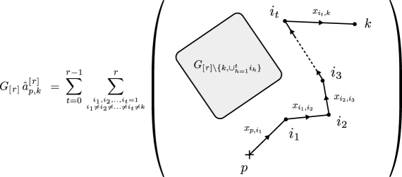
Figure 4: Pictorial interpretation of $G_{[r]}\,\hat{a}_{p,k}^{[r]}$. The starting point of the oriented open path, $p$, belongs to the set $\{r+1,r+2,...,n\}$.

From here we also explicitly see that the pole coefficient $\hat{a}_{p,k}^{[r]}$ is charged under the $U(1)^{n}$ subgroup of the gauge group of the quiver. Since every $G_{[r]}$ has zero $U(1)^{n}$ charge, and the product of $x_{ab}$ coefficients $x_{p,i_{1}}x_{i_{1},i_{2}}x_{i_{2},i_{3}}\cdots x_{i_{t-1},i_{t}}x_{i_{t},k}$ is charged under the $p$-th $U(1)$ and the $k$-th $U(1)$ as $(-1,1)$ respectively, the whole quantity $\hat{a}_{p,k}^{[r]}$ will carry a $(-1,1)$ charge under $U(1)_{p}\times U(1)_{k}$, just like an $x_{p,k}$ variable would. These quantities are also helpful in writing down a recursive formula for $G_{[r]}$. Note that $G_{[r+1]}$ can be written as

$$G_{[r+1]} =G_{[r]}\left(1-x_{r+1,r+1}-\sum_{k=1}^{r}\hat{a}_{r+1,k}^{[r]}\,x_{k,r+1}\right)$$

$$=G_{[r]}\left(1-x_{r+1,r+1}\right)-\sum_{k=1}^{r}G_{[r]}\,\hat{a}_{r+1,k}^{[r]}\,x_{k,r+1}\,.$$ (4.26)

The terms in the sum above are of the form (4.25), so that we can use it to bring $G_{[r+1]}$ into the form

$$G_{[r+1]} =G_{[r]}\left(1-x_{r+1,r+1}\right)$$

$$\qquad\qquad-\sum_{k=1}^{r}\sum_{t=0}^{r-1}\sum^{r}_{i_{1},i_{2},..,i_{t}=1\atop i_{1}\neq i_{2}\neq...\neq i_{t}\neq k}G_{[r]\setminus\{k,\cup_{h=1}^{t}i_{h}\}}x_{r+1,i_{1}}x_{i_{1},i_{2}}x_{i_{2},i_{3}}\cdots x_{i_{t-1},i_{t}}x_{i_{t},k}x_{k,r+1}\,,$$ (4.27)

and after relabelling some summation variables, we can write the this equation as

$$G_{[r+1]} =G_{[r]}-G_{[r]}x_{r+1,r+1}$$

$$\qquad\qquad-\sum_{t=1}^{r}\sum^{r}_{i_{1},i_{2},..,i_{t}=1\atop i_{1}\neq i_{2}\neq...\neq i_{t}}G_{[r]\setminus\{\cup_{h=1}^{t}i_{h}\}}x_{r+1,i_{1}}x_{i_{1},i_{2}}x_{i_{2},i_{3}}\cdots x_{i_{t-1},i_{t}}x_{i_{t},r+1}\,,$$ (4.28)

and since the second term on the RHS of this identity is just the $t=0$ term of the following sum, we finally have

$$G_{[r+1]} =G_{[r]}-\sum_{t=0}^{r}\sum^{r}_{i_{1},i_{2},..,i_{t}=1\atop i_{1}\neq i_{2}\neq...\neq i_{t}}G_{[r]\setminus\{\cup_{h=1}^{t}i_{h}\}}x_{r+1,i_{1}}x_{i_{1},i_{2}}x_{i_{2},i_{3}}\cdots x_{i_{t-1},i_{t}}x_{i_{t},r+1}\,.$$ (4.29)

We can also give a similar formula for each of the $H_{l}$ coefficients in the product (4.23). We know that

$$H_{l}(\vec{x})=\left(1-x_{{{l}},{{l}}}-\sum_{q=1}^{l-1}\hat{a}_{{l},q}^{[l-1]}\,x_{q,{{l}}}\right)^{-1}\,,$$ (4.30)

and using $F^{[n]}_{0}=G_{[n]}^{-1}$ we can write

$$H_{l}(\vec{x}) =\left(1-F^{[l-1]}_{0}G_{[l-1]}x_{{l},{l}}-F^{[l-1]}_{0}\sum_{q=1}^{l-1}G_{[l-1]}\,\hat{a}_{l,q}^{[l-1]}\,x_{q,{l}}\right)^{-1}$$

$$=\left(1-F^{[l-1]}_{0}\left(G_{[l-1]}x_{{l},{l}}+\sum_{q=1}^{l-1}G_{[l-1]}\,\hat{a}_{l,q}^{[l-1]}\,x_{q,{l}}\right)\right)^{-1}\,.$$ (4.31)

We again get have terms like $G_{[l-1]}\,\hat{a}_{l,q}^{[l-1]}\,x_{q,l}$, which have the same structure of the ones encountered in the derivation of eq. (4.29). We can just redo the same steps done previously to bring the equation for the $H_{l}(\vec{x})$ coefficient into the form

$$H_{l}(\vec{x}) =\left(1-F^{[l-1]}_{0}\,\sum_{t=0}^{l-1}\sum^{l-1}_{i_{1},i_{2},..,i_{t}=1\atop i_{1}\neq i_{2}\neq...\neq i_{t}}G_{[l-1]\setminus\{\cup_{h=1}^{t}i_{h}\}}x_{l,i_{1}}x_{i_{1},i_{2}}x_{i_{2},i_{3}}\cdots x_{i_{t-1},i_{t}}x_{i_{t},l}\right)^{-1}$$

$$=F_{0}^{[l-1]}\,\left(G_{[l-1]}-\sum_{t=0}^{l-1}\sum^{l-1}_{i_{1},i_{2},..,i_{t}=1\atop i_{1}\neq i_{2}\neq...\neq i_{t}}G_{[l-1]\setminus\{\cup_{h=1}^{t}i_{h}\}}x_{l,i_{1}}x_{i_{1},i_{2}}x_{i_{2},i_{3}}\cdots x_{i_{t-1},i_{t}}x_{i_{t},l}\right)^{-1}$$

$$=\frac{G_{[l-1]}}{G_{[l]}}\,,$$ (4.32)

where in the last step we used eq. (4.29). We can then rewrite eq. (4.23) as

$$F^{[n]}_{0}=\prod_{i=1}^{n}H_{i}(\vec{x})=\prod_{i=1}^{n}\frac{G_{[i-1]}}{G_{[i]}}\,,$$ (4.33)

with $G_{[0]}=1$.

4.1 $F_{0}^{[n]}$ and the sum over subsets

In this section we will prove the expression for $\left(F_{0}^{[n]}\right)^{-1}$ given in [1]

$$\left(F_{0}^{[n]}\right)^{-1}=1+\sum_{\mathbb{V}\subseteq V_{n}}\,\sum_{\sigma\in\text{Sym}(\mathbb{V})}(-1)^{C_{\sigma}}y_{\sigma}(\{x_{ab}\})\,,$$ (4.34)

where $\mathbb{V}$ is any subset of the set of nodes $V_{n}=\{1,2,...,n\}$ of the quiver but the empty set, and $\text{Sym}(\mathbb{V})$ is the group of all the permutations of elements in $\mathbb{V}$. $C_{\sigma}$ is the number of cycles in $\sigma$. $y_{\sigma}(\{x_{ab}\})$ is a monomial built from the $x_{ab}$ coefficients as

$$y_{\sigma}(\{x_{ab}\}) =\prod_{i}y_{\sigma^{(i)}}(\{x_{ab}\})\,,$$ (4.35)

where the product runs over the cycles $\sigma^{(i)}$ of the permutation $\sigma=\prod_{i}\sigma^{(i)}$, and for a single cycle $(i_{1},i_{2},\cdots,i_{k})$

$$y_{(i_{1},i_{2},...i_{k})}(\{x_{ab}\})=x_{i_{1},i_{2}}x_{i_{2},i_{3}}\cdots x_{i_{k},i_{1}}\,.$$ (4.36)

For example, when $\sigma=(12)(3)$, the permutation which swaps $1$ and $2$ and leaves $3$ fixed, then $y_{(12)(3)}(\{x_{ab}\})=x_{12}x_{21}x_{33}$. This equation has thus an interpretation in terms of loops $\{y_{c}\}$ on a complete quiver, where each loop $y_{c}$ corresponds to a cycle $c=(i_{1},\cdots,i_{k})$ as in (4.36). Since these loops corresponds to cyclic permutations, they do not visit the same node more than once: for this reason we call them simple loops, to distinguish them from more general closed paths. In the following we will write the above formula as $\tilde{G}_{[n]}$ :

$$\tilde{G}_{[n]}=1+\sum_{\mathbb{V}\subseteq V_{n}}\,\sum_{\sigma\in\text{Sym}(\mathbb{V})}(-1)^{C_{\sigma}}y_{\sigma}(\{x_{ab}\})\,.$$ (4.37)

To prove the identity (4.34) we will show that the sequence $\tilde{G}_{[n]}$ obeys the same recursion relation (4.29) satisfied by the $G_{[n]}$ coefficients obtained from the residue computations. We have

$$\tilde{G}_{[n+1]}=1+\sum_{\mathbb{V}\subset\{1,\cdots,n+1\}}\sum_{\sigma\in Sym(\mathbb{V})}(-1)^{C_{\sigma}}y_{\sigma}\,.$$ (4.38)

If the subset $\mathbb{V}$ of $\{1,\cdots,n+1\}$ does not include $n+1$, we have a sum which, together with the leading $1$, gives $G_{[n]}$. The remaining terms involve subsets which include the $\{n+1\}$ node. For such subsets, the permutation $\sigma$ can either be of the product form $\sigma^{\prime}(n+1)$, where $\sigma^{\prime}$ is a permutation of $\{1,\cdots,n\}$ and $(n+1)$ is a single cycle of length one, or alternatively it is of the form $\sigma^{\prime}(i_{1},i_{2},\cdots,i_{k},n+1)$, with $\sigma^{\prime}$ a permutation of $\{1,\cdots,n\}\setminus\{i_{1},\cdots,i_{k}\}$ and $(i_{1},\cdots,i_{k},n+1)$ a cycle of length $k+1$. The first type of term gives

$$-\tilde{G}_{[n]}y_{n+1}=-\tilde{G}_{[n]}x_{n+1,n+1}\,.$$ (4.39)

The second type of term gives

$$-\sum_{k=1}^{n}\sum_{i_{1}\neq i_{2}\neq\cdots\neq i_{k}=1}^{n}\tilde{G}_{[n]\setminus\{i_{1},\cdots,i_{k}\}}y_{i_{1},\cdots,i_{k},n+1}\,.$$ (4.40)

Collecting the terms we find

$$\tilde{G}_{[n+1]}=\tilde{G}_{[n]}(1-x_{n+1,n+1})-\sum_{k=1}^{n}\sum_{i_{1}\neq i_{2}\neq\cdots i_{k}=1}^{n}\tilde{G}_{[n]\setminus\{i_{1},\cdots,i_{k}\}}x_{i_{1}i_{2}}x_{i_{2}i_{3}}\cdots x_{i_{k},n+1}x_{n+1,i_{1}}\,.$$ (4.41)

This proves that the guessed formula $\tilde{G}_{[n]}$ satisfies the same recursion relation as $G_{[n]}$. It is evident that $G_{[1]}=\tilde{G}_{[1]}=1$. This proves that $\tilde{G}_{[n]}=G_{[n]}$, $\forall\,n$.

4.2 $F_{0}^{[n]}$ and determinants

Equation (4.34) can be used to recast $F^{[n]}_{0}(\{x_{ab}\})$ as a determinant expression given by

$$F^{[n]}_{0}(\{x_{ab}\})=\frac{1}{\det\left(\mathbb{1}_{n}-X_{n}\right)}\,,$$ (4.42)

where $\mathbb{1}_{n}$ is the $n$ dimensional identity matrix and $X_{n}$ is a $n\times n$ matrix defined by

$$\left.X_{n}\right|_{ij}=x_{ij}\,,\qquad 1\leq(i,j)\leq n\,.$$ (4.43)

The following identity for the expansion of $\det(\mathbb{1}_{n}-X_{n})$ in terms of sub-determinants of $X_{n}$, or equivalently characters of $X_{n}$ associated with single-column Young diagrams, is useful:

$$\det\left(\mathbb{1}_{n}-X_{n}\right) =\sum_{k=0}^{n}(-1)^{k}\chi_{[1^{k}]}(X_{n})$$ (4.44)

$$=\sum_{k=0}^{n}{(-1)^{k}}\sum_{i_{1},i_{2},...,i_{k}=1}^{n}\,\sum_{\sigma\in S_{k}}\,\frac{(-1)^{\sigma}}{k!}x_{i_{1}i_{\sigma(1)}}x_{i_{2}i_{\sigma(2)}}\cdots x_{i_{k}i_{\sigma(k)}}\,.$$ (4.45)

This expansion is organized according to the number of $1$’s picked up from the matrix $(\mathbb{1}_{n}-X_{n})$ in calculating its determinant. When we pick $n-k$ of the $1$’s, we have the sum of the sub-determinants constructed from blocks of size $k$ from the matrix $X_{n}$. When we pick $n-k$ of these $1$ valued entries, we have the sum of the sub-determinants constructed from blocks of size $k$ from the matrix $X_{n}$. The sign $(-1)^{\sigma}$ is the parity of the permutation. Because of the antisymmetrisation $\sum_{\sigma}(-1)^{\sigma}$, the sum over $i_{1},i_{2},...,i_{k}$ can be restricted to run over the set $i_{1}\neq i_{2}\neq...\neq i_{k}$, so that it can be rewritten as a sum over subsets $\mathbb{V}_{k}$ of $k$ different integers from $\{1,\cdots,n\}$. For each choice of subset there is factor of $k!$ for ways of assigning $i_{1},\cdots,i_{k}$ to the elements of the subset. Hence

$$\det\left(\mathbb{1}_{n}-X_{n}\right)=\sum_{k=0}^{n}(-1)^{k}\sum_{\mathbb{V}_{k}}\sum_{\sigma\in Sym\left(\mathbb{V}_{k}\right)}(-1)^{k-C_{\sigma}}y_{\sigma}\,.$$ (4.46)

$Sym(\mathbb{V}_{k})$ is the symmetric group of permutations of elements in $\mathbb{V}_{k}$. Here we have used the fact that the parity of a permutation $\sigma$ can be written in terms of the number of cycles as $(-1)^{\sigma}=(-1)^{k-C_{\sigma}}$ and we also used the definition of $y_{\sigma}$. The expression (4.34) now follows.

4.3 Word counting and the building block $F_{0}^{[n]}$

The generating function $\mathcal{Z}(\{x_{ab;\alpha}\})$ for gauge invariant operators for unflavoured quiver theories has been given as an infinite product built from a building block $F_{0}^{[n]}(\{x_{ab}\})$. This has been expressed in terms of a determinant of the matrix $(\mathbb{1}_{n}-X_{n})$, where $(X_{n})|_{ab}=x_{ab}$.

After expanding $F_{0}^{[n]}(\{x_{ab}\})$ in a power series in the variables $x_{ab}$, it is natural to ask if the coefficients in this series have a combinatoric interpretation as counting something. The answer does not immediately follow from the combinatoric interpretation of $\mathcal{Z}(\{x_{ab;\alpha}\})$ in terms of gauge invariants, nevertheless, the coefficients in the expansion of $F_{0}^{[n]}(\{x_{ab}\})$ are themselves positive. This follows from the Cauchy-Littlewood formula for the expansion of the inverse determinant:

$${1\over\det(\mathbb{1}_{n}-X_{n})}=\sum_{k=0}^{\infty}{1\over k!}\sum_{i_{1}\cdots i_{k}=1}^{n}\sum_{\sigma\in S_{k}}x_{i_{1},i_{\sigma(1)}}x_{i_{2},i_{\sigma(2)}}\cdots x_{i_{k},i_{\sigma(k)}}\,.$$ (4.47)

This strongly suggests that there should be a combinatoric interpretation in terms of properties of graphs. We will find that there are in fact two combinatoric interpretations: both in terms of word counting related to the quiver with one directed edge for every specified start and end-point. We will call the latter the complete $n$-node quiver. We will refer to these two as the charge conserving open string word (COSW) counting problem and the closed string word (CSW) counting problem. It turns out that the equivalence between these two word counting problems is a known mathematical result! This gives a new connection between word counting problems and gauge theory.

To motivate the CSW interpretation, let us take the simple case of $n=2$, for which we have

$$F_{0}^{[2]}(x_{11},x_{12},x_{21},x_{22})={1\over(1-x_{11}-x_{22}-x_{12}x_{21}+x_{11}x_{22})}\,.$$ (4.48)

The denominator depends on variables

$$y_{11}=x_{11}\,,\qquad\quad y_{12}=x_{12}x_{21}\,,\qquad\quad y_{22}=x_{22}\,.$$ (4.49)

These variables are associated with closed loops in a graph with two nodes, and one edge for every pair of specified starting and end points. Let us first set $y_{12}=0$: we have

$${1\over(1-y_{11}-y_{22}+y_{11}y_{22})}={1\over(1-y_{11})}{1\over(1-y_{22})}\,.$$ (4.50)

Expanding in powers of $y_{11},y_{22}$, we see

$${1\over(1-y_{11}-y_{22}+y_{11}y_{22})}=\sum_{m_{1}=0}^{\infty}y_{11}^{m_{1}}\sum_{m_{2}=0}^{\infty}y_{22}^{m_{2}}\,.$$ (4.51)

We describe the CSW interpretation in this simple case. Take the letters $\hat{y}_{11},\hat{y}_{22}$ and consider arbitrary strings of these, with the condition that

$$\hat{y}_{11}\hat{y}_{22}=\hat{y}_{22}\hat{y}_{11}\,.$$ (4.52)

A general word is characterized by the number $m_{11}$ and $m_{22}$ of $\hat{y}_{11},\hat{y}_{22}$. With these numbers specified, the commutation relation can be used to write any such word as

$$(\hat{y}_{11})^{m_{11}}(\hat{y}_{22})^{m_{22}}\,.$$ (4.53)

There is thus, precisely one word with content $(m_{11},m_{22})$. Thus the coefficient of $y_{11}^{m_{11}}y_{22}^{m_{22}}$ is equal to the number of words in a language made from letters $\hat{y}_{11},\hat{y}_{22}$. The words are sequences of these letters, with the commutation relation (4.52). Now set $y_{11}=0$

$$F_{0}^{[2]}(y_{11}=0,y_{12},y_{22}) ={1\over(1-y_{12}-y_{22})}=\sum_{m=0}^{\infty}(y_{12}+y_{22})^{m}=\sum_{m=0}^{\infty}\sum_{m_{12}=0}^{m}{m!\over m_{12}!m_{22}!}y_{12}^{m_{12}}y_{22}^{m_{22}}$$

$$=\sum_{m_{22}=0}^{\infty}\sum_{m_{12}=0}^{\infty}{(m_{12}+m_{22})!\over m_{12}!m_{22}!}y_{12}^{m_{12}}y_{22}^{m_{22}}\,.$$ (4.54)

In this case, we can consider letters $\hat{y}_{12},\hat{y}_{22}$, without imposing the commutation condition. Then a general word with specified numbers $m_{12},m_{22}$ is the number of sequences we can write with $m_{12},m_{22}$ copies of $\hat{y}_{12},\hat{y}_{22}$. Each word corresponds to one way of placing the $m_{12}$ objects of one kind and $m_{22}$ objects of another kind in $m_{12}+m_{22}$ positions. This shows that the number of words is ${(m_{12}+m_{22})!\over m_{12}!m_{22}!}$ in agreement with the coefficient above.

These simple examples illustrate a general interpretation of all the coefficients in the expansion of $F_{0}^{[n]}$, in terms of the cycle variables $y_{c}$. Consider the complete $n$-node quiver. To each simple closed loop $c$ on the graph, associate a variable $\hat{y}_{c}$. If we label the nodes of the graph $\{1,\cdots,n\}$, every cyclic permutation of a subset of the nodes corresponds to a simple loop on the graph. These simple loops visit each node no more than once. To define the CSWs, we associate a letter to $\hat{y}_{c}$ to every simple loop. We impose the relation

$$\hat{y}_{c}\hat{y}_{c^{\prime}}=\hat{y}_{c^{\prime}}\hat{y}_{c}$$ (4.55)

for every pair of simple loops $c,\,c^{\prime}$ that have no node in common. The letters which do share a node are treated as non-commuting, while the letters that do not share a node are treated as commutative. Then we consider strings containing $m_{c}$ copies of the letter $\hat{y}_{c}$. A simple guess, based on the above examples, is that the coefficient of $\prod_{c}y_{c}^{m_{c}}$ in the expansion of $F_{0}^{[n]}$ is exactly equal to the number of distinct words build from the letters $\hat{y}_{c}$ with specified numbers $m_{c}$ for each letter. This word counting interpretation is called closed string word counting since the loops can be thought as closed strings made from open strings which are the edges extending between nodes. The validity of this interpretation will be explained by using its equivalence to an open string word counting.

Appendix E gives more examples of direct checks of this connection between closed string word counting and the building block function $F_{0}^{[n]}$.

From the derivation of the generating function of gauge invariants we know that

$$F^{[n]}_{0}(\{x_{ab}\}) =\frac{1}{\det(\mathbb{1}_{n}-X_{n})}=\sum_{\vec{p}\,}\,\prod_{a=1}^{n}\left(\sum_{b=1}^{n}p_{ab}\right)!\left(\prod_{b=1}^{n}\frac{x_{ab}^{\,p_{ab}}}{p_{ab}!}\right)\delta\left(\sum_{b=1}^{n}(p_{ab}-p_{ba})\right)\,.$$ (4.56)

This gives another way to see that the coefficients in the expansion are positive, and in fact integers. Consider the coefficient of $\prod_{a,b}x_{ab}^{p_{ab}}$, which is

$$\prod_{a}\,\frac{\left(\sum_{b=1}^{n}p_{ab}\right)!}{\prod_{b=1}^{n}p_{ab}!}\,\delta\left(\sum_{b=1}^{n}(p_{ab}-p_{ba})\right)\,.$$ (4.57)

This leads directly to the open string word counting. Consider letters $\hat{x}_{ab}$ corresponding to each directed edge, going from $a$ to $b$ in the complete $n$-node quiver. We will call these open string bits. Then consider words which are sequences of these letters. These words will be called open string words. We impose the commutation condition

$$\hat{x}_{ab}\hat{x}_{a^{\prime}b^{\prime}}=\hat{x}_{a^{\prime}b^{\prime}}\hat{x}_{ab}$$ (4.58)

for $a\neq a^{\prime}$. So sequences which differ by such a swap are counted as the same word. Thus, string bits which have different starting points do not commute. Two different string bits with the same starting point do not commute. For each starting point $a$ the factor

$$\frac{\left(\sum_{b=1}^{n}p_{ab}\right)!}{\prod_{b=1}^{n}p_{ab}!}\,$$ (4.59)

counts the number of sequences containing $p_{ab}$ copies of $\hat{x}_{ab}$. Defining

$$p_{a}=\sum_{b}p_{ab}=\sum_{b}p_{ba}\,,$$ (4.60)

an open string word will take the form

$$w_{o}=\hat{x}_{1a_{1}}\hat{x}_{1a_{2}}\cdots\hat{x}_{1a_{p_{1}}}~{}~{}~{}\hat{x}_{2a_{p_{1}+1}}\hat{x}_{2a_{p_{1}+2}}\cdots\hat{x}_{2a_{p_{1}+p_{2}}}~{}~{}\cdots~{}~{}\hat{x}_{na_{p_{1}+\cdots+p_{n-1}+1}}\cdots\hat{x}_{na_{p_{1}+\cdots+p_{n}}}\,.$$ (4.61)

The open string bits with different starting points commute, so we have used that commutativity to place all the ones starting at $1$ to the far left, the ones starting from $2$ next, and so on. The integers $a_{1},\cdots,a_{\sum_{i}p_{i}}$ will contain $p_{1}$ copies of $1$, $p_{2}$ copies of $2$ etc. This condition says that the sequence of open string bits that appear in the expansion of $F_{0}^{[n]}$ contains as many bits with starting point $i$ as with end points as $i$. We will refer to this as charge conserving open string words. So we have shown that the $F_{0}^{[n]}$ counts charge-conserving open string words. Remarkably, Cartier and Foata proved that charge-conserving open string words are in 1-1 correspondence with closed string words ! This is theorem 3.5 in Cartier-Foata [23].

We refer the reader to [23] for the formal proof. Here we explain, with examples, the meaning of this equivalence between the counting of charge-conserving open string words (COSW) and closed string words (CSW). Given an a CSW, it is easy to write down a corresponding COSW. Take for example

$$\hat{y}_{11}\,\hat{y}_{12}\,\hat{y}_{11}\,\hat{y}_{22}\,\hat{y}_{123}=\hat{y}_{11}\,\hat{y}_{12}\,\hat{y}_{22}\,\hat{y}_{11}\,\hat{y}_{123}\,.$$ (4.62)

Write these closed-string letters in terms of open string bits:

$$\hat{y}_{11}=\hat{x}_{11}\,,\quad\,\,\hat{y}_{22}=\hat{x}_{22}\,,\quad\,\,\hat{y}_{12}=\hat{x}_{12}\hat{x}_{21}\,,\quad\,\,\hat{y}_{123}=\hat{x}_{12}\hat{x}_{23}\hat{x}_{31}\,.$$ (4.63)

The word of interest becomes

$$\hat{x}_{11}\hat{x}_{12}\hat{x}_{21}\hat{x}_{11}\hat{x}_{22}\hat{x}_{12}\hat{x}_{23}\hat{x}_{31}=\hat{x}_{11}\hat{x}_{12}\hat{x}_{11}\hat{x}_{12}~{}~{}\hat{x}_{21}\hat{x}_{22}\hat{x}_{23}~{}~{}\hat{x}_{31}\,.$$ (4.64)

We have used the commutativity to arrange as in (4.61). A CSW determines in this way a unique COSW.

The reverse is also true. A COSW determines a unique CSW. The general proof is non-trivial [23]. We just illustrate with some examples here. Consider some COSW with specified numbers of starting (and end-) points of particular types, say three starting and ending at $1$, two at $2$ and three at $3$. These words are of the form

$$\hat{x}_{1,\tau(1)}\hat{x}_{1,\tau(1)}\hat{x}_{1,\tau(1)}~{}~{}~{}\hat{x}_{2,\tau(2)}\hat{x}_{2,\tau(2)}~{}~{}~{}\hat{x}_{3,\tau(3)}\hat{x}_{3,\tau(3)}\hat{x}_{3,\tau(3)}\,.$$ (4.65)

Here $\tau$ is a permutation in $S_{8}$, which should be thought of as moving the integers $\{1,2,3\}$ from their initial positions $(1,1,1,2,2,3,3,3)$ to a new position. When $\tau$ is the identity we have the COSW

$$\hat{x}_{11}\hat{x}_{11}\hat{x}_{11}~{}~{}\hat{x}_{22}\hat{x}_{22}~{}~{}~{}\hat{x}_{33}\hat{x}_{33}\hat{x}_{33}=\hat{y}_{11}\hat{y}_{11}\hat{y}_{11}~{}~{}\hat{y}_{22}\hat{y}_{22}~{}~{}~{}\hat{y}_{33}\hat{y}_{33}\hat{y}_{33}\,.$$ (4.66)

Suppose now $\tau=(1,2,3,4,5,6,7,8)$, a cyclic permutation. The COSW is

$$\hat{x}_{13}\hat{x}_{11}\hat{x}_{11}~{}~{}\hat{x}_{21}\hat{x}_{22}~{}~{}~{}\hat{x}_{32}\hat{x}_{33}\hat{x}_{33}\,.$$ (4.67)

If we map this to closed string words, this will involve two copies of $\hat{y}_{11}$, two copies of $\hat{y}_{33}$, and $\hat{y}_{132}=\hat{x}_{13}\hat{x}_{32}\hat{x}_{21}$. The unique CSW is

$$\hat{y}_{132}~{}~{}\hat{y}_{11}\hat{y}_{11}~{}~{}\hat{y}_{22}~{}~{}\hat{y}_{33}\hat{y}_{33}\,.$$ (4.68)

In arriving at this, we did a re-arrangement which moves the $\hat{x}_{32}$ across the $\hat{x}_{22}$. This is allowed, since the open string bits commute when they have different strating point. i.e. different first index. The reader is encouraged to play with different choices of $\tau$. It is easy to see that permutations $\tau$ in $S_{8}$ are a somewhat redundant way to parametrize the COSW. In fact it is a coset of $S_{8}$ by $S_{3}\times S_{2}\times S_{3}$ that parametrizes the COSW. For any choice of $\tau$, there is always a CSW, i.e a list of $\hat{y}_{c}$ for different cycles, arranged in a specific order (modulo the commutation relations (4.55)), which agrees with the COSW after re-arrangements allowed by the commutation (4.58). This is guaranteed by theorem 3.5 of [23].

We have focused on the combinatoric interpretation of $F_{0}^{[n]}(\{x_{ab}\})$, in terms of the complete quiver graph. This basic building block generates the counting of gauge invariants at large $N$ for any quiver, after taking an infinite product with the substitutions in (2.2). If we are interested in a quiver where there is no edge going from $a$ to $b$, these substitutions involve setting $x_{ab}\rightarrow 0$ for that pair of nodes. It is instructive to consider the quantity

$$\mathcal{F}_{0}^{[n]}(\{x_{ab;\alpha}\})=F_{0}^{[n]}(\{x_{ab}\rightarrow\sum_{\alpha}x_{ab,\alpha}\})\,,$$ (4.69)

which is not an infinite product, but knows about the connectivity of any chosen quiver graph, with general multiplicities (possibly zero) between any specified start and end-node. This quantity has an interpretation in terms of word counting of open string words, as it follows immediately from (4.56):

$$\mathcal{F}^{[n]}_{0}(\{x_{ab,\alpha}\}) =\sum_{\vec{p}\,}\,\prod_{a=1}^{n}\left(\sum_{b=1}^{n}\sum_{\alpha=1}^{M_{ab}}p_{ab,\alpha}\right)!\left(\prod_{b=1}^{n}\,\prod_{\alpha=1}^{M_{ab}}\frac{x_{ab,\alpha}^{\,p_{ab,\alpha}}}{p_{ab,\alpha}!}\right)\delta\left(\sum_{b=1}^{n}\sum_{\alpha=1}^{M_{ab}}(p_{ab,\alpha}-p_{ba,\alpha})\right)\,.$$ (4.70)

We again have the basic rule that different open string letters corresponding to string bits with the same starting point do not commute. Again by invoking the Cartier-Foata theorem we see that, for any quiver, it is possible to map the open word counting problem to a closed word counting problem, in which string letters corresponding to simple loops which share a node do not commute.

The building block $F_{0}^{[n]}(\{x_{ab}\})$ gives the counting of gauge invariants at large $N$, by means of a simple combinatoric operation involving an infinite product and elementary substitutions. One of our motivations for developing a combinatorial interpretation for $F_{0}^{[n]}(\{x_{ab}\})$, is that it highlights an interesting analogy with a deformation of the counting problems considered here. We have focused on the counting of all holomorphic invariants made from chiral fields in an $\mathcal{N}=1$ theory. In many of the $\mathcal{N}=1$ theories of interest in AdS/CFT, the general holomorphic invariants form the chiral ring in the limit of zero superpotential, but beyond that, one wants to impose super-potential relations. In these cases, the counting of chiral gauge invariant operators leads to the $N$-fold symmetric product of the ring of functions on non-compact Calabi-Yau spaces [36]. In the large $N$ limit, the plethystic exponential gives the counting in terms of the counting at $N=1$. The $N=1$ counting is a simple building block of the large $N$ counting. It has a physical interpretation as the ring of functions on the CY and the plethystic exponential has an interpreation in terms of the bosonic statistics of many identical branes.

The procedure of taking an infinite product and making substitutions, that we have developed for the $N\rightarrow\infty$ counting at zero superpotential, can be viewed as an analog of the plethystic exponential. In this analogy the function $F_{0}^{[n]}(\{x_{ab}\})$ corresponds to the $U(1)$ counting, which is the same as counting holomorphic functions on a CY. The counting problems we have solved also correspond to some large $N$ geometries: namely the spaces of multiple matrices, subject to gauge invariance constraints. There is no symmetric product structure in this geometry, but there is nevertheless a simple analog of the plethystic exponential. There is no physical interpretation of $F_{0}^{[n]}(\{x_{ab}\})$ as a gauge theory partition function, but there is nevertheless an interpretation in terms of string word counting partially commuting string letters. A deeper understanding and interpretation of these analogies will undoubtedly be fascinating.

5 The flavoured case: from contour integrals to a determinant expression

We now turn to the full picture, that is we allow for quarks and antiquarks. Take then eq. (3.28):

$$F^{[n]}(\{x_{ab}\},\{t_{a}\},\{\bar{t}_{a}\})=\left(\prod_{a}\oint_{\mathcal{C}_{a}}\frac{dz_{a}}{2\pi i}\right)\prod_{a}\,I_{a}(x_{ab},t_{a},\bar{t}_{a})\,,$$ (5.1)

where

$$I_{a}(\vec{z};\vec{x}_{a},t_{a},\bar{t}_{a})=\cfrac{\exp\left(z_{a}t_{a}\right)}{z_{a}-\left(\bar{t}_{a}+\sum\limits_{b=1}^{n}z_{b}\,x_{b,a}\right)}\,.$$ (5.2)

Again we have to compute residues. First of all note that the numerator of (5.2) is regular in $z_{a}$, so that the only poles may come from its denominator. We can simplify the next steps by using a trick: let us rename $\bar{t}_{a}\equiv x_{0,a}$ and multiply it by a dummy variable, $z_{0}$. Pictorially, this would consist of taking all the open (fundamental matter) edges in the quiver and joining them to a fictitious node, that we call $`0$ node’. For consistency, let us also rename $t_{a}\equiv x_{a,0}$ . Using this notation we can rewrite eq. (5.2) as

$$I_{a}(\vec{z};\vec{x}_{a},t_{a},\bar{t}_{a})=\cfrac{\exp\left(z_{a}\,x_{a,0}\right)}{z_{a}-\left(z_{0}\,x_{0,a}+\sum\limits_{b=1}^{n}z_{b}\,x_{b,a}\right)}=\cfrac{\exp\left(z_{a}\,x_{a,0}\right)}{z_{a}-\left(\sum\limits_{b=0}^{n}z_{b}\,x_{b,a}\right)}\,.$$ (5.3)

where it is understood that $z_{0}$ will be set to $1$ after the $z_{i}$ ($1\leq i\leq n$) integrals have been done. This means that the intermediate expressions arising from successive integrations will take the same form as in the unflavoured case of Section 4. In particular the pole prescription still holds unaltered.

With this formalism, eq. (4.12) becomes

$$z_{j}^{*[r]}=z_{j}^{*}(z_{r+1},...,z_{n},z_{0};\vec{x})=\sum_{i>r\atop\cup\{i=0\}}z_{i}\,\hat{a}_{i,j}^{[r]}\,,$$ (5.4)

and correspondingly eq. (4) gets modified as

$$\left(1-\left(x_{{r+1},{r+1}}+\sum_{i=1}^{r}\hat{a}_{r+1,i}^{[r]}\,x_{i,{r+1}}\right)\right)z_{r+1}=$$

$$\qquad\qquad\qquad=\sum_{j>{r+1}\atop\cup\{j=0\}}z_{j}\left(x_{j,{r+1}}+\sum_{i=1}^{r}\hat{a}_{j,i}^{[r]}\,x_{i,{r+1}}\right)\,.$$ (5.5)

We can then proceed in the exact same fashion as in section 4. The only manifestly different piece in the integrand are the numerators of (5.3). To highlight the similarity to the unflavoured case, we write

$$\tilde{I}_{a}(\vec{z};\vec{x}_{a})=\frac{1}{\displaystyle z_{a}-\left(x_{0,a}+\sum\limits_{b=1}^{n}z_{b}\,x_{b,a}\right)}\equiv\frac{1}{\displaystyle z_{a}-\sum\limits_{b=0}^{n}z_{b}\,x_{b,a}}\,.$$ (5.6)

such that

$$I_{a}(\vec{z};\vec{x}_{a},t_{a},\bar{t}_{a})=\cfrac{\exp(z_{a}t_{a})}{z_{a}-\left(\bar{t}_{a}+\sum\limits_{b=1}^{n}z_{b}\,x_{b,a}\right)}\equiv\exp(z_{a}\,x_{a,0})\,\tilde{I}_{a}(\vec{z};\vec{x}_{a})\,.$$ (5.7)

For the flavoured case the equation corresponding to (4.15) would then be

$$F^{[n]} =\prod_{j=1}^{r}H_{j}(\vec{x})\,\left(\prod_{a>r}^{n}\oint_{\mathcal{C}_{a}}\frac{dz_{a}}{2\pi i}\right)\,\left(\prod_{k=1}^{r}\exp\left(z_{k}^{*[r]}\,x_{k,0}\right)\right)$$

$$\qquad\qquad\qquad\times\prod_{a>r}\,\tilde{I}_{a}(z_{1}^{*[r]},z_{2}^{*[r]},...,z_{r}^{*[r]},z_{r+1},z_{r+2},...,z_{n};\vec{x}_{a})\,\exp(z_{a}x_{a,0})\,,$$ (5.8)

where in exact analogy with (4.22)

$$H_{j}(\vec{x})=\left(1-\left(x_{{j},{j}}+\sum_{i=1}^{j-1}\hat{a}_{j,i}^{[j-1]}\,x_{i,{j}}\right)\right)^{-1}\,.$$ (5.9)

Again, we see that the only addition in comparison to the unflavoured case is the product over the exponential functions. After the $n$ integrations have been done, using the definition in eq. (5.4), we have

$$z_{k}^{*[n]}=z_{k}^{*}(z_{0};\vec{x}_{k})=\sum_{i>n\atop\cup\{i=0\}}z_{i}\,\hat{a}_{i,k}^{[n]}\equiv z_{0}\,\hat{a}_{0,k}^{[n]}\,.$$ (5.10)

At this point we set $z_{0}=1$. Eq. (5.10) becomes

$$z_{k}^{*[n]}=\hat{a}_{0,k}^{[n]}\,,$$ (5.11)

so that

$$\prod_{k=1}^{n}\exp\left(z_{k}^{*[n]}\,x_{k,0}\right)=\prod_{k=1}^{r}\exp{\left(\hat{a}_{0,k}^{[n]}\,x_{k,0}\right)}\,.$$ (5.12)

We can then say that $F$ is the product

$$F^{[n]}=\prod_{j=1}^{n}H_{j}(\vec{x})\,\exp\left(z_{j}^{*[n]}\,x_{j,0}\right)=\prod_{j=1}^{n}\left(\frac{\displaystyle\exp{\left(\hat{a}_{0,j}^{[n]}\,x_{j,0}\right)}}{\displaystyle 1-x_{{j},{j}}-\sum_{i=1}^{j-1}\hat{a}_{j,i}^{[j-1]}\,x_{i,{j}}}\right)\,,$$ (5.13)

where $x_{p,0}=t_{p}$ and $x_{0,p}=\bar{t}_{p}$. As expected, by setting all the fundamental matter field chemical potentials to zero we return to the unflavoured case.

In Appendix F we show that the numerator of this formula has the form

$$\exp\left(\sum_{j=1}^{n}\hat{a}_{0,j}^{[n]}t_{j}\right)=\exp\left(\sum_{p,q=1}^{n}\,t_{p}\bar{t}_{q}\,\frac{(-1)^{p+q}\,M_{p,q}}{\det(\mathbb{1}_{n}-X_{n})}\right)\,,$$ (5.14)

where $M_{p,q}$ is the $(p,q)$ minor of the matrix $(\mathbb{1}_{n}-X_{n})$. We can then write

$$F^{[n]}=\frac{1}{\det(\mathbb{1}_{n}-X_{n})}\,\exp\left(\sum_{p,q=1}^{n}\,t_{p}\bar{t}_{q}\,\,\frac{(-1)^{p+q}\,M_{p,q}}{\det(\mathbb{1}_{n}-X_{n})}\right)\,.$$ (5.15)

A second expression for the same quantity was also given in Appendix F, and it reads

$$F^{[n]}=F^{[n]}_{0}\,\exp\left(t_{p}\bar{t}_{q}\,\partial^{p,q}\,\log F_{0}^{[n]}\vphantom{\sum}\right)\,,$$ (5.16)

where we used Einstein summation on $p,q$, and $\partial^{p,q}=\frac{\partial}{\partial x_{pq}}$.

Note that, as in the unflavoured case, we can write $F^{[n]}$ as a determinant of a suitable matrix, which encodes all the information of the quiver under study. Since

$$\frac{(-1)^{p+q}\,M_{p,q}}{\det(\mathbb{1}_{n}-X_{n})}=\left.\left(\mathbb{1}_{n}-X_{n}\right)^{-1}\right|_{q,p}\,,$$ (5.17)

if we introduce the $n\times n$ matrices $\chi_{n}$ and $\Lambda_{n}$, defined by

$$\left.\chi_{n}\right|_{p,q}=\left.(\mathbb{1}_{n}-X_{n})^{-1}\right|_{p,q}\,,\qquad\left.\Lambda_{n}\right|_{p,q}=t_{p}\bar{t}_{q}\,,$$ (5.18)

then we can write

$$F^{[n]}(\{x_{ab}\},\{t_{a}\},\{\bar{t}_{a}\})=\det\chi_{n}\,\exp\left[\text{Tr}\left(\chi_{n}\,\Lambda_{n}\right)\right]\,.$$ (5.19)

Finally, the last equation can be put in the determinant form

$$F^{[n]}(\{x_{ab}\},\{t_{a}\},\{\bar{t}_{a}\})=\det\left(\chi_{n}\,\exp\left[\chi_{n}\,\Lambda_{n}\right]\right)\,.$$ (5.20)

The generating function $\mathcal{Z}$ is obtained from $F$ using eq. (3.1). However, from e.g. eq. (5.20) we see that $t_{a},\bar{t}_{b}$ always appear pairwise, so that we can rewrite (3.1) in the more symmetric form already anticipated in eq. (2.2), that is

$${\mathcal{Z}}( \{x_{ab,\alpha}\},\{\mathcal{T}_{a,\beta}\},\{\bar{\mathcal{T}}_{a,\gamma}\})$$

$$=\prod_{i}F^{[n]}\left(\left\{x_{ab}\rightarrow\sum_{\alpha}x_{ab,\alpha}^{i}\right\},\left\{t_{a}\rightarrow\sum_{\beta}\frac{\text{Tr}(\mathcal{T}_{a,\beta}^{\,i})}{\sqrt{i}}\right\},\left\{\bar{t}_{a}\rightarrow\sum_{\gamma}\frac{\text{Tr}(\bar{\mathcal{T}}_{a,\gamma}^{\,i})}{\sqrt{i}}\right\}\right)\,\,.$$ (5.21)

This is the final expression for our large $N$ generating function.

6 Some examples

We will now present some simple applications of our counting formulae, for the large $N$ limit.

6.1 One node quiver

Rewriting the chemical potentials of the fields as $x_{11}\rightarrow x,\,t_{1}\rightarrow t,\,\bar{t}_{1}\rightarrow\bar{t}$, we have

$$\chi_{1}=\frac{1}{1-x}\,,\qquad\quad\Lambda_{1}=t\bar{t}\,,$$ (6.1)

so that

$$F^{[1]}=\det(\chi_{1}\exp[\chi_{1}\Lambda_{1}])=\det(\chi_{1})\,\exp\left[\text{Tr}(\chi_{1}\Lambda_{1})\right] =\cfrac{e^{\cfrac{t\bar{t}}{1-x}}}{1-x}\,.$$ (6.2)

The large $N$ generating function is then

$$\mathcal{Z}(\{x_{\alpha}\},\{\mathcal{T}_{\beta}\},\{\bar{\mathcal{T}}_{\gamma}\})=\prod_{i}\cfrac{\exp\left(\cfrac{{\sum_{\beta,\gamma}\text{Tr}(\mathcal{T}_{\beta}^{i})\,\text{Tr}(\bar{\mathcal{T}}_{\gamma}^{i})}}{{i(1-\sum_{\alpha}x_{\alpha}^{i})}}\right)}{1-\sum_{\alpha}x_{\alpha}^{i}}\,.$$ (6.3)

For the $d=4$, $\mathcal{N}=4$ SYM theory with quiver shown in Figure 5

Figure 5: $d=4$, $\mathcal{N}=4$ SYM quiver

the $\mathcal{Z}$ function is

$$\mathcal{Z}_{SYM}(x_{1},x_{2},x_{3})=\prod_{i}\frac{1}{1-x_{1}^{i}-x_{2}^{i}-x_{3}^{i}}\,.$$ (6.4)

For the SQCD model, described by the quiver

Figure 6: $d=4$ $\mathcal{N}=1$ SQCD quiver

the generating function is instead

$$\mathcal{Z}_{SQCD}(\mathcal{T},\bar{\mathcal{T}})=\prod_{i}\exp\left\{\frac{1}{i}\,\text{Tr}(\mathcal{T}^{i})\,\text{Tr}(\bar{T}^{i})\right\}=\prod_{j=1}^{F}\prod_{k=1}^{\bar{F}}\left(1-t_{j}\bar{t}_{k}\right)^{-1}\,,$$ (6.5)

where we used

$$\mathcal{T}=\text{diag}(t_{1},t_{2},...,t_{F})\,,\qquad\quad\bar{\mathcal{T}}=\text{diag}(\bar{t}_{1},\bar{t}_{2},...,\bar{t}_{\bar{F}})\,.$$ (6.6)

Note that if in the last example we do not distinguish the $U(1)\subset U(F)$ charges of the quarks and the $U(1)\subset U(\bar{F})$ charges of the antiquarks, that is we set $\mathcal{T}=t\,\mathbb{1}_{F}$ and $\bar{T}=\bar{t}\,\mathbb{1}_{\bar{F}}$, we get

$$\mathcal{Z}_{SQCD}(t\,\mathbb{1}_{F},\bar{t}\,\mathbb{1}_{\bar{F}})=(1-t\bar{t}\,)^{-F\bar{F}}\,,$$ (6.7)

which was already derived in [37], using different counting methods.

An interesting gauge theory can be obtained by adding fundamental matter to $\mathcal{N}=4$ SYM [18, 19]. This operation breaks half of the supersymmetries leaving an $\mathcal{N}=2$ theory, which in turn we can describe with the $\mathcal{N}=1$ quiver [38] in figure 7

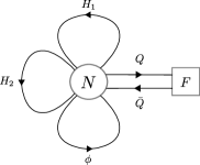
Figure 7: $\mathcal{N}=2$ SQCD with and adjoint hypermultiplet.

The $\mathcal{N}=2$ theory has a vector multiplet $\mathcal{V}$ (1 complex scalar $\phi$) and an hypermultiplet $\mathcal{H}$ (two complex scalars $H_{1},\,H_{2}$) both in the adjoint of $U(N)$. A second hypermultiplet $\mathcal{Q}$ is in the bifundamental $U(N)\times U(F)$, where $U(F)$ is a global (non-dynamical) flavour symmetry (two complex scalars $Q,\,\bar{Q}$, transforming in opposite way under the symmetry group). The large $N$ generating function for this quiver, that we denote by $\mathcal{Z}_{\mathcal{N}=2}(x_{1},x_{2},x_{3},\mathcal{T},\bar{\mathcal{T}})$, is given by

$$\mathcal{Z}_{\mathcal{N}=2}(x_{1},x_{2},x_{3},\mathcal{T},\bar{\mathcal{T}})=\prod_{i}\cfrac{\exp\left[\cfrac{\text{Tr}(\mathcal{T}^{i})\,\text{Tr}(\bar{\mathcal{T}}^{i})}{i\left(1-x_{1}^{i}-x_{2}^{i}-x_{3}^{i}\right)}\right]}{1-x_{1}^{i}-x_{2}^{i}-x_{3}^{i}}\,.$$ (6.8)

The first terms in the expansion of the unrefined $\mathcal{Z}_{\mathcal{N}=2}(x_{1},x_{2},x_{3},t\,\mathbb{1}_{F},\bar{t}\,\mathbb{1}_{F})$ read

$$\mathcal{Z}_{\mathcal{N}=2}(x_{1},x_{2},x_{3},t\,\mathbb{1}_{F},\bar{t}\, \mathbb{1}_{F})=1+x_{1}+x_{2}+x_{3}+F^{2}t\bar{t}+2x_{1}x_{2}+2x_{1}x_{3}+2x_{2}x_{3}+2F^{2}t\bar{t}x_{1}$$

$$+2F^{2}t\bar{t}x_{2}+2F^{2}t\bar{t}x_{3}+6\,x_{1}x_{2}x_{3}+\frac{F^{2}}{2}\left(1+F^{2}\right)t^{2}\bar{t}^{2}$$ (6.9)

$$+6F^{2}t\bar{t}x_{1}x_{2}+6F^{2}t\bar{t}x_{1}x_{3}+6F^{2}t\bar{t}x_{2}x_{3}+\frac{F^{2}}{2}\left(1+3F^{2}\right)t^{2}\bar{t}^{2}x_{1}+...$$

Let us now check explicitly the validity of our generating function for some of these coefficients, in the large $N$ limit. Let us start off by considering just one quark/antiquark pair and one adjoint scalar, say $H_{1}$. The Gauge Invariant Operators (GIOs) we can build out of these fields are

$$(\phi)(\bar{Q}Q)^{k}_{l}\,,\qquad\,(\bar{Q}\,\phi\,Q)^{k}_{l}\,,$$ (6.10)

where upper and lower indices belong to the fundamental and antifundamental of $U(F)$ and $U(\bar{F})$ respectively, and round brackets denote $U(N)$ indices contraction. The total number of GIOs for this given configuration is $2F^{2}$. We see that this value is the same one of the coefficient $t\bar{t}x_{1}$, so that we have a first test of the validity of (6.1). Consider now the situation in which we only have two pairs of quarks/antiquarks. The only GIOs we can form are of the form

$$(\bar{Q}Q)^{k_{1}}_{l_{1}}\,(\bar{Q}Q)^{k_{2}}_{l_{2}}\,,$$ (6.11)

using the same convention of the example above for the flavour and gauge indices. This is just a product of two matrix elements of the same $F$ dimensional matrix $(\bar{Q}Q)$. The total number of inequivalent GIOs is then $\frac{1}{2}F^{2}\left(1+F^{2}\right)$: once again this is the same coefficient of the term $(t\bar{t})^{2}$ in (6.1). As a last example, suppose added to the last configuration a single field $\phi$. The GIOs we can form would then be

$$(\phi)\,(\bar{Q}Q)^{k_{1}}_{l_{1}}\,(\bar{Q}Q)^{k_{2}}_{l_{2}}\,,\qquad(\bar{Q}\,\phi\,Q)^{k_{1}}_{l_{1}}\,(\bar{Q}Q)^{k_{2}}_{l_{2}}\,.$$ (6.12)

The one on the left consists brings a total of $\frac{F^{2}}{2}\left(1+F^{2}\right)$ GIOs, while the one on the right adds another $F^{2}$ GIOs to the final quantity, which then reads

$$\frac{F^{2}}{2}\left(1+F^{2}\right)+F^{2}=\frac{F^{2}}{2}\left(1+3F^{2}\right)\,,$$ (6.13)

In agreement with the coefficient of $(t\bar{t})^{2}x_{1}$ in (6.1).

6.2 Two node quiver

We now present some two-node quiver examples. From the definitions in (2.6) we can immediately write

$$\chi_{2}=\left(\mathbb{1}_{2}-X_{2}\right)^{-1}=\frac{1}{\det\left(\mathbb{1}_{2}-X_{2}\right)}\left(\begin{array}[]{ll}1-x_{22}&x_{12}\\ x_{21}&1-x_{11}\end{array}\right)\,,$$ (6.14)

and

$$\Lambda_{2}=\left(\begin{array}[]{ll}t_{1}\bar{t}_{1}&t_{1}\bar{t}_{2}\\ t_{2}\bar{t}_{1}&t_{2}\bar{t}_{2}\end{array}\right)\,;$$ (6.15)

so that, from (2.8):

$$F^{[2]} =\det(\chi_{2}\exp[\chi_{2}\Lambda_{2}])=\det(\chi_{2})\exp[\text{Tr}(\chi_{2}\Lambda_{2})]$$

$$=\cfrac{\exp\left(\cfrac{t_{1}\bar{t}_{1}(1-x_{22})+t_{1}\bar{t}_{2}x_{21}+t_{2}\bar{t}_{1}x_{12}+t_{2}\bar{t}_{2}(1-x_{11})}{1-x_{11}-x_{22}-x_{12}x_{21}+x_{11}x_{22}}\right)}{1-x_{11}-x_{22}-x_{12}x_{21}+x_{11}x_{22}}\,.$$ (6.16)

Finally, recalling (2.2), we can get the large $N$ generating function from $F^{[2]}$ by mapping

$$x_{11}\rightarrow\sum_{\alpha=1}^{M_{11}}x_{11,\alpha}^{i}\,,\qquad x_{12}\rightarrow\sum_{\alpha=1}^{M_{12}}x_{12,\alpha}^{i}\,,\qquad x_{21}\rightarrow\sum_{\alpha=1}^{M_{21}}x_{21,\alpha}^{i}\,,\qquad x_{22}\rightarrow\sum_{\alpha=1}^{M_{22}}x_{22,\alpha}^{i}\,,$$ (6.17a)

$$t_{k}\rightarrow i^{-1/2}\sum_{\beta=1}^{M_{k}}\text{Tr}(\mathcal{T}_{k,\beta}^{i})\,,\,\,\,\,k=1,2\,,\qquad\bar{t}_{k}\rightarrow i^{-1/2}\sum_{\gamma=1}^{\bar{M}_{k}}\text{Tr}(\bar{\mathcal{T}}_{k,\gamma}^{i})\,,\,\,\,\,k=1,2\,,$$ (6.17b)

and by taking the product over $i$ from 1 to $\infty$.

The most famous two-node quiver is Klebanov and Witten’s conifold gauge theory, consisting of the gauge group $U(N)\times U(N)$ and four bifundamental fields: two of them, $A_{1}$ and $A_{2}$, in the representation $(\bar{\Box},\,\Box)$ and the remaining two, $B_{1}$ and $B_{2}$, in the representation $(\Box,\,\bar{\Box})$ of the gauge group. Here we consider the deformation of such a model obtained by allowing flavour symmetries, which is sometimes called ‘flavoured conifold’ [21, 22, 34, 35]

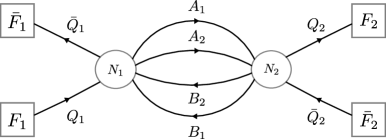
Figure 8: The flavoured conifold gauge theory.

We now choose a different notation for the chemical potentials of the fields, to accord to more standard conventions:

$$\begin{array}[]{lllll}&x_{12,1}\rightarrow a_{1}\,,&x_{12,2}\rightarrow a_{2}\,,&x_{21,1}\rightarrow b_{1}\,,&x_{21,2}\rightarrow b_{2}\,,\\[8.53581pt] &\mathcal{T}_{1,1}\rightarrow q_{1}\,,&\mathcal{T}_{2,1}\rightarrow q_{2}\,,&\bar{\mathcal{T}}_{1,1}\rightarrow\bar{q}_{1}\,,&\bar{\mathcal{T}}_{2,1}\rightarrow\bar{q}_{2}\,.\end{array}$$

The first terms in the power expansion of $\mathcal{Z}_{\text{Flavoured}\atop\text{ Conifold}}(a_{1},a_{2},b_{1},b_{2},q_{1},q_{2},\bar{q}_{1},\bar{q}_{2})$ in the large $N$ limit then read

$$\mathcal{Z}_{\text{Flavoured}\atop\text{ Conifold}}= 1+a_{1}b_{1}+2a_{1}^{2}b_{1}^{2}+2a_{1}^{2}b_{1}b_{2}+2a_{2}a_{1}b_{1}^{2}+a_{1}b_{2}+2a_{2}^{2}b_{1}^{2}+a_{2}b_{1}+a_{2}b_{2}+\text{Tr}_{F_{1}}(q_{1})\text{Tr}_{\bar{F}_{1}}(\bar{q}_{1})$$

$$+2a_{1}b_{1}\text{Tr}_{F_{1}}(q_{1})\text{Tr}_{\bar{F}_{1}}(\bar{q}_{1})+2a_{2}b_{1}\text{Tr}_{F_{1}}(q_{1})\text{Tr}_{\bar{F}_{1}}(\bar{q}_{1})+4a_{1}^{2}b_{1}^{2}\text{Tr}_{F_{1}}(q_{1})\text{Tr}_{\bar{F}_{1}}(\bar{q}_{1})$$

$$+6a_{1}a_{2}b_{1}^{2}\text{Tr}_{F_{1}}(q_{1})\text{Tr}_{\bar{F}_{1}}(\bar{q}_{1})+a_{1}\text{Tr}_{F_{1}}(q_{1})\text{Tr}_{\bar{F}_{2}}(\bar{q}_{2})+12a_{1}a_{2}b_{1}b_{2}\text{Tr}_{F_{1}}(q_{1})\text{Tr}_{\bar{F}_{1}}(\bar{q}_{1})+...$$

6.3 Three node quiver: $dP_{0}$

The del Pezzo $dP_{0}$ gauge theory (obtained from $D3$ branes on $\mathbb{C}_{3}/\mathbb{Z}_{3}$ orbifold singularities [39]) contains nine bifundamental fields charged under the $U(N_{1})\times U(N_{2})\times U(N_{3})$ gauge group as represented in the following quiver, in which we also added flavour symmetry:

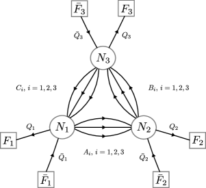
Figure 9: Flavoured $dP_{0}$ gauge theory.

We refer to this theory as the flavoured $dP_{0}$ theory. Using the convention for the chemical potentials of the fields

$$\begin{array}[]{llllll}&x_{12,1}\rightarrow a_{1}\,,&x_{12,2}\rightarrow a_{2}\,,&x_{12,3}\rightarrow a_{3}\,,&\mathcal{T}_{1,1}\rightarrow q_{1}\,,&\bar{\mathcal{T}}_{1,1}\rightarrow\bar{q}_{1}\,,\\[8.53581pt] &x_{23,1}\rightarrow b_{1}\,,&x_{23,2}\rightarrow b_{2}\,,&x_{23,3}\rightarrow b_{3}\,,&\mathcal{T}_{2,1}\rightarrow q_{2}\,,&\bar{\mathcal{T}}_{2,1}\rightarrow\bar{q}_{2}\,,\\[8.53581pt] &x_{31,1}\rightarrow c_{1}\,,&x_{31,2}\rightarrow c_{2}\,,&x_{31,3}\rightarrow c_{3}\,,&\mathcal{T}_{3,1}\rightarrow q_{3}\,,&\bar{\mathcal{T}}_{3,1}\rightarrow\bar{q}_{3}\,,\\[8.53581pt] \end{array}$$

we can write the generating function for the flavoured $dP_{0}$ theory in the large $N$ limit as:

$$\mathcal{Z}_{dP_{0}\text{ Flav.}}=\prod_{i}\,\frac{1}{1-\sum\limits_{j,k,l=1}^{3}(a_{j}\,b_{k}\,c_{l})^{i}}$$

$$\times\exp\left(\frac{\text{Tr}_{F_{1}}(q_{1}^{i})\left(\text{Tr}_{\bar{F}_{1}}(\bar{q}_{1}^{i})+\text{Tr}_{\bar{F}_{3}}(\bar{q}_{3}^{i})\sum\limits_{p=1}^{3}a_{p}^{i}+\text{Tr}_{\bar{F}_{2}}(\bar{q}_{2}^{i})\sum\limits_{p,q=1}^{3}c_{p}^{i}a_{q}^{i}\right)}{i\left(1-\sum\limits_{j,k,l=1}^{3}(a_{j}\,b_{k}\,c_{l})^{i}\right)}\right.$$

$$\qquad\qquad\left.+\frac{\text{Tr}_{F_{2}}(q_{2}^{i})\left(\text{Tr}_{\bar{F}_{2}}(\bar{q}_{2}^{i})+\text{Tr}_{\bar{F}_{1}}(\bar{q}_{1}^{i})\sum\limits_{p=1}^{3}b_{p}^{i}+\text{Tr}_{\bar{F}_{3}}(\bar{q}_{3}^{i})\sum\limits_{p,q=1}^{3}b_{p}^{i}a_{q}^{i}\right)}{i\left(1-\sum\limits_{j,k,l=1}^{3}(a_{j}\,b_{k}\,c_{l})^{i}\right)}\right.$$

$$\qquad\qquad\qquad\left.+\frac{\text{Tr}_{F_{3}}(q_{3}^{i})\left(\text{Tr}_{\bar{F}_{3}}(\bar{q}_{3}^{i})+\text{Tr}_{\bar{F}_{2}}(\bar{q}_{2}^{i})\sum\limits_{p=1}^{3}c_{p}^{i}+\text{Tr}_{\bar{F}_{1}}(\bar{q}_{1}^{i})\sum\limits_{p,q=1}^{3}b_{p}^{i}c_{q}^{i}\right)}{i\left(1-\sum\limits_{j,k,l=1}^{3}(a_{j}\,b_{k}\,c_{l})^{i}\right)}\right)\,.$$ (6.19)

7 Summary and outlook

In this paper, we have revisited the counting of local holomorphic operators in general quiver gauge theories with bi-fundamental fields, which was started in [1] (see also related recent work [40]), focusing on the infinite product formula obtained for the limit of large $N$. This was extended to flavoured quivers, which include fundamental matter. The flavoured quivers have gauge nodes and flavour nodes. The gauge nodes are associated with unitary group factors in the gauge symmetry. The flavour nodes are associated with unitary global symmery factors. We used Schur-Weyl duality relating the representation theory of unitary groups to permutation groups in order to convert integrals over the gauge unitary groups for the counting into permutation sums. The sums involved multiple permutations with constraints. These constraints were expressed by introducing contour integrals. This lead to an analogous infinite product formula for these flavoured quivers (2.2). For any quiver with $n$ gauge nodes, all the factors in the infinite product are obtained by substitutions in one function $F^{[n]}(\{x_{ab}\},\{t_{a}\},\{\bar{t}_{a}\})$, with $a,b$ ranging over the $n$ nodes. The building block $F^{[n]}(\{x_{ab}\},\{t_{a}\},\{\bar{t}_{a}\})$ was found to be closely related to $F_{0}^{[n]}(\{x_{ab}\})$. The determinant and cofactors of the matrix $(\mathbb{1}_{n}-X_{n})$ played a prominent role in these formulae. We also obtained results for the counting of local operators at finite $N$ in terms of Young diagrams and Littlewood-Richardson coefficients.

The permutation group-theoretic counting of operators at finite $N$ is the first step in the construction of an orthogonal basis of operators for an inner product related to two-point functions between holomorphic and anti-holomorphic operators in free field theory [1]. The next step is the computation of three and higher point functions in the free theory. The orthogonal bases were found to be given by simple rules involving Young diagrams and related group theoretic multiplicities attached to the quiver diagram itself. Three-point functions were given by cutting and gluing of the diagrams. The counting and the construction of the orthogonal bases were given in terms of two-dimensional topological field theories (TFT2) of Dijkgraaf-Witten type, based on permutations and equipped with appropriate defects. Given the close similarity we have found between the counting formulae for flavoured and unflavoured quivers, we expect that the results on orthogonal bases, correlators and TFT2 [1] will also have simple generalizations from unflavoured quivers to flavoured quivers. An interesting avenue would be to explore the links between this permutation group TFT2 approach to correlators with methods based on integrable models (see e.g [41, 42]).

The flavoured counting at large $N$ is determined by $F^{[n]}$, which is closely related to $F_{0}^{[n]}$, which in turn we have related to word counting problems associated to the complete $n$-node quiver. One formulation of the word counting problem was in terms of words made from letters corresponding to simple closed loops on the quiver. The letters do not commute if they share a node, otherwise they commute. In another formulation, the letters correspond to edges of the quiver. Distinct letters do not commute if they share a starting point. These open string bits form words, a subset of which obey a charge conservation condition. A non-trivial combinatoric equivalence between the open string and closed string counting problems is given by the Cartier-Foata theorem. In this paper, we have come across these string-word-counting problems in connection with the counting formula for gauge invariants. It is natural to ask if such words, and their monoidal structure, are relevant beyond the counting of gauge theory invariants. One often finds that mathematical structures relevant to counting a class of objects are also relevant in the understanding of the interactions of such objects (see e.g. [33, 43] for a concrete application of this idea). Do the string-words found here play a role in interactions, namely in the computation of correlators of gauge-invariant operators in the free field limit and at weak coupling? Since the work of Cartier-Foata has subsequently been related to statistical physics models [31, 44], this underlying mathematical structure could reveal new connections between four dimensional gauge theory and statistical physics.

In the context of AdS/CFT, comparisons between the counting of a class of local gauge-invariant operators and the spectrum of brane fluctuations was initiated in [18, 19, 20]. These papers considered the simplest quiver gauge theory, namely $N=4$ SYM, and the additional fundamental matter corresponds to the addition of $7$-branes in the dual $AdS_{5}\times S^{5}$ background. The results presented here should be useful for generalizations of these results, such as increasing the number of $7$-branes, and more substantially, going beyond the $N=4$ SYM as starting point to more general quiver theories. The finite $N$ aspects of counting, where operators are labelled by Young diagrams, should be related to giant gravitons. This will require the investigation of $3$-brane giant gravitons in $AdS_{5}\times S^{5}$, in the presence of the probe $7$-branes. Some discussion of such configurations is initiated in the conclusions of [45]. Such detailed comparisons for the general class of flavoured quiver theories we considered here would undoubtedly deepen our understanding of AdS/CFT.

In this paper we have counted general holomorphic gauge invariant operators in quiver theories with fundamental matter. These also form the space of chiral operators in the theory in the absence of a superpotential. When we turn on a superpotential, equivalence classes related by setting to zero the derivatives of the super-potential, form the chiral ring [46, 47]. This jump in the spectrum of chiral primaries has been discussed in the context of AdS/CFT in [48]. An important future direction is to understand this jump in quantitative detail. We have found that the quiver diagram defining a theory contains powerful information on the counting of operators in the theory, and the weighted adjacency matrix played a key role in giving a general form for the generating functions at large $N$. It would be interesting to look for analogous general formulae, involving the weighted adjacency matrix, along with the superpotential data, for the case of chiral rings at non-zero superpotential. In a similar vein we may ask if indices in superconformal theories, for general quivers, can be expressed in terms of the weighted adjacency matrix. It will be interesting to investigate this theme in existing examples of index computations for quivers (e.g. [49, 50, 51]). Beyond counting questions, the transition to non-zero superpotential poses the question of the exact form of BPS operators. In cases where the 1-loop dilatation operator is known, such as $\mathcal{N}=4$ SYM, we can find the BPS operators by solving for the null eigenstates among the holomorphic operators. Partial results at large $N$ as well as finite $N$, building on the knowledge of free field bases of operators, are available in [7, 8, 33, 43, 52, 53, 54, 55]. A similar treatment should be possible for orbifolds of $\mathcal{N}=4$.

The counting of chiral operators with and without superpotential is of interest in studying the Hilbert series of moduli spaces arising from super-symmetric gauge-theories [37, 56, 57]. These moduli spaces often have an interpretation in terms of branes. Quiver gauge theories, with and without fundamental matter, have been studied in this context. The formulae obtained here, for finite $N$ as well as large $N$, will be expected to have applications in the study of these moduli spaces. Another potential application of the present counting techniques is in the thermodynamics of AdS/CFT or toy models thereof, e.g. [58].

Acknowledgements

We thank Robert de Mello Koch, Yang-Hui He, Vishnu Jejjala, James McGrane, Gabriele Travaglini and Brian Wecht for useful discussions. SR is supported by STFC consolidated grant ST/L000415/1 “String Theory, Gauge Theory & Duality.” PM is supported by a Queen Mary University of London studentship.

Appendix A Generating function

A.1 Derivation of the generating function

In this appendix we will derive eq. (3.1). Our starting point will be eq. (3.14):

$$\mathcal{Z} (\{x_{ab,\alpha}\},\{\mathcal{T}_{a,\beta}\},\{\bar{\mathcal{T}}_{a,\gamma}\})=\sum_{\{n_{ab,\alpha}\}}\,\sum_{\{n_{a,\beta}\}\atop\{\bar{n}_{a,\gamma}\}}\,\left(\prod_{a,b,\alpha}\,x_{ab,\alpha}^{n_{ab,\alpha}}\right)\,\sum_{\left\{R_{a}\vdash n_{a}\atop l(R_{a})\leq N_{a}\right\}}\,\sum_{\{r_{ab,\alpha}\vdash n_{ab,\alpha}\}}\,\sum_{\{r_{a,\beta}\vdash n_{a,\beta}\}\atop\{\bar{r}_{a,\gamma}\vdash\bar{n}_{a,\gamma}\}}$$ (A.1)

$$\prod_{a}\,g(\cup_{b,\alpha}r_{ab,\alpha}\cup_{\beta}r_{a,\beta};R_{a})\,g(\cup_{b,\alpha}r_{ba,\alpha}\cup_{\gamma}\bar{r}_{a,\gamma};R_{a})\ \left(\prod_{\beta}\chi_{r_{a,\beta}}(\mathcal{T}_{a,\beta})\right)\left(\prod_{\gamma}\chi_{\bar{r}_{a,\gamma}}(\bar{\mathcal{T}}_{a,\gamma})\right)\,,$$

in which we will take the large $N$ limit, in such a way that we will be allowed to drop the constraints on the sums over $R_{a}$. The derivation will involve well known symmetric group identities. In particular, we will use the equation

$$\chi_{R}(U)=\sum_{\sigma\in S_{n}}\frac{\chi_{R}(\sigma)}{n!}\prod_{i}\,(\text{Tr}\,U^{i})^{[\sigma]^{(i)}}\,,\qquad U\in U(F)$$ (A.2a)

where $$R n [\sigma]^{(i)} i [\sigma] \sigma\in S_{n} \text{Tr}(U) U(F)$$ is a partition of , is the number of cycles of length in the conjugacy class of the permutation and is the trace taken in the fundamental representation of . We will also use the formulae

$$\quad\sum_{R\vdash n}\chi_{R}(\sigma)\chi_{R}(\tau)=\sum_{\gamma\in S_{n}}\delta(\gamma\sigma\gamma^{-1}\tau^{-1})\,,$$ (A.2b)

and

$$\quad g(\cup_{a}r_{a};R)=\left(\prod_{a}\sum_{\sigma_{a}}\right)\chi_{R}(\times_{a}\sigma_{a}){\prod_{a}\frac{\chi_{r_{a}}(\sigma_{a})}{n_{a}!}}\,.$$ (A.2c)

Here $r_{a}$ are partitions of $n_{a}$ and $\delta(\sigma)$ is the symmetric group delta function, which equals one iff $\sigma$ is the identity permutation. With these relations we can rewrite $\mathcal{Z}$ in (A.1) as

$$\mathcal{Z}= \sum_{\vec{n}}\,\sum_{\vec{\sigma},\,\vec{\sigma}^{\prime}}\,\prod_{a}\,\left(\prod_{b,\alpha}\sum_{r_{ab,\alpha}}\frac{x_{ab,\alpha}^{\sum_{i}i[\sigma_{ab,\alpha}]^{(i)}}}{(n_{ab,\alpha}!)^{2}}\,\chi_{r_{ab,\alpha}}(\sigma_{ab,\alpha})\chi_{r_{ab,\alpha}}(\sigma^{\prime}_{ab,\alpha})\right)$$

$$\quad\times\left(\prod_{\beta}\sum_{r_{a,\beta}}\frac{\prod_{i}(\text{Tr}\,\mathcal{T}_{a,\beta}^{\,i})^{[\sigma_{a,\beta}]^{(i)}}}{(n_{a,\beta}!)^{2}}\chi_{r_{a,\beta}}(\sigma_{a,\beta})\chi_{r_{a,\beta}}(\sigma^{\prime}_{a,\beta})\right)$$

$$\qquad\qquad\times\left(\prod_{\gamma}\sum_{r_{a,\gamma}}\frac{\prod_{i}(\text{Tr}\,\bar{\mathcal{T}}_{a,\gamma}^{\,i})^{[\bar{\sigma}_{a,\gamma}]^{(i)}}}{(\bar{n}_{a,\gamma}!)^{2}}\chi_{\bar{r}_{a,\gamma}}(\bar{\sigma}_{a,\gamma})\chi_{\bar{r}_{a,\gamma}}(\bar{\sigma}^{\prime}_{a,\gamma})\right)$$

$$\qquad\qquad\qquad\times\sum_{R_{a}}\,\chi_{R_{a}}(\times_{b,\alpha}\sigma_{ab,\alpha}\times_{\beta}\sigma_{a,\beta}^{\prime})\chi_{R_{a}}(\times_{b,\alpha}\sigma^{\prime}_{ba,\alpha}\times_{\gamma}\bar{\sigma}_{a,\gamma}^{\prime})\,,$$ (A.3)

where we defined

$$\vec{\sigma}=\cup_{a,b,\alpha}\{\sigma_{ab,\alpha}\}\cup_{a,\beta}\{\sigma_{a,\beta}\}\cup_{a,\gamma}\{\bar{\sigma}_{a,\gamma}\}\,,$$

$$\sigma_{ab,\alpha}\in S_{n_{ab,\alpha}}\,,\qquad\sigma_{a,\beta}\in S_{n_{a,\beta}}\,,\qquad\bar{\sigma}_{a,\gamma}\in S_{\bar{n}_{a,\gamma}}\,,$$ (A.4)

and similarly

$$\vec{n}=\cup_{a,b,\alpha}\{n_{ab,\alpha}\}\cup_{a,\beta}\{n_{a,\beta}\}\cup_{a,\gamma}\{\bar{n}_{a,\gamma}\}\,.$$ (A.5)

Summing over the representations $R_{a},r_{ab,\alpha},r_{a,\beta},\bar{r}_{a,\gamma}$ then gives, using (A.2b)

$$\mathcal{Z}=\sum_{\vec{n}} \,\sum_{\vec{\sigma},\,\vec{\sigma}^{\prime}}\sum_{\vec{\rho}}\,\prod_{a}\left(\prod_{b,\alpha}\frac{x_{ab,\alpha}^{\sum_{i}i[\sigma_{ab,\alpha}]^{(i)}}}{(n_{ab,\alpha}!)^{2}}\,\delta\left(\rho_{ab,\alpha}\,\sigma_{ab,\alpha}\,\rho_{ab,\alpha}^{-1}\,{\sigma^{\prime\,-1}_{ab,\alpha}}\right)\right)$$

$$\quad\times\left(\prod_{\beta}\frac{\prod_{i}(\text{Tr}\,\mathcal{T}_{a,\beta}^{\,i})^{[\sigma_{a,\beta}]^{(i)}}}{(n_{a,\beta}!)^{2}}\,\delta\left(\rho_{a,\beta}\,\sigma_{a,\beta}\,\rho_{a,\beta}^{-1}\,{\sigma^{\prime\,-1}_{a,\beta}}\right)\right)$$

$$\qquad\times\left(\prod_{\gamma}\frac{\prod_{i}(\text{Tr}\,\bar{\mathcal{T}}_{a,\gamma}^{\,i})^{[\bar{\sigma}_{a,\gamma}]^{(i)}}}{(\bar{n}_{a,\gamma}!)^{2}}\delta\left(\bar{\rho}_{a,\gamma}\,\bar{\sigma}_{a,\gamma}\,\bar{\rho}_{a,\gamma}^{-1}\,{{{\bar{\sigma}}_{a,\gamma}}}^{\prime\,-1}\right)\right)$$

$$\qquad\quad\times\sum_{\Gamma_{a}}\delta\left(\Gamma_{a}(\times_{b,\alpha}\sigma_{ab,\alpha}\times_{\beta}\sigma_{a,\beta}^{\prime})\Gamma_{a}^{-1}{(\times_{b,\alpha}\sigma^{\prime}_{ba,\alpha}\times_{\gamma}\bar{\sigma}_{a,\gamma}^{\prime})}^{-1}\right)\,,$$ (A.6)

with

$$\vec{\rho}=\cup_{a,b,\alpha}\{\rho_{ab,\alpha}\}\cup_{a,\beta}\{\rho_{a,\beta}\}\cup_{a,\gamma}\{\bar{\rho}_{a,\gamma}\}\,,$$

$$\rho_{ab,\alpha}\in S_{n_{ab,\alpha}}\,,\qquad\rho_{a,\beta}\in S_{n_{a,\beta}}\,,\qquad\bar{\rho}_{a,\gamma}\in S_{\bar{n}_{a,\gamma}}\,.$$ (A.7)

If we now sum over the $\vec{\sigma}^{\prime}$ permutations we get, redefining the dummy $\Gamma_{a}$ permutations as $\Gamma_{a}\rightarrow\left(\times_{b,\alpha}\rho_{ba,\alpha}\times_{\gamma}\bar{\rho}_{a,\gamma}\right)\Gamma_{a}\left(\times_{b,\alpha}1\times_{\beta}\rho_{a,\beta}\right)^{-1}$ :

$$\mathcal{Z}=\sum_{\vec{n}}\,\sum_{\vec{\sigma},\,\vec{\rho}}\,\prod_{a} \left(\prod_{b,\alpha}\frac{x_{ab,\alpha}^{\sum_{i}i[\sigma_{ab,\alpha}]^{(i)}}}{(n_{ab,\alpha}!)^{2}}\right)\left(\prod_{\beta}\frac{\prod_{i}(\text{Tr}\,\mathcal{T}_{a,\beta}^{\,i})^{[\sigma_{a,\beta}]^{(i)}}}{(n_{a,\beta}!)^{2}}\right)\left(\prod_{\gamma}\frac{\prod_{i}(\text{Tr}\,\bar{\mathcal{T}}_{a,\gamma}^{\,i})^{[\bar{\sigma}_{a,\gamma}]^{(i)}}}{(\bar{n}_{a,\gamma}!)^{2}}\right)$$

$$\qquad\times\sum_{\Gamma_{a}}\,\delta\left(\Gamma_{a}(\times_{b,\alpha}\sigma_{ab,\alpha}\times_{\beta}\sigma_{a,\beta})\Gamma_{a}^{-1}{(\times_{b,\alpha}\sigma_{ba,\alpha}\times_{\gamma}\bar{\sigma}_{a,\gamma})}^{-1}\right)\,.$$ (A.8)

Finally, by summing over the now trivial $\vec{\rho}$ permutations we obtain

$$\mathcal{Z}=\sum_{\vec{n}}\,\sum_{\vec{\sigma}}\prod_{a} \left(\prod_{b,\alpha}\frac{x_{ab,\alpha}^{\sum_{i}i[\sigma_{ab,\alpha}]^{(i)}}}{n_{ab,\alpha}!}\right)\left(\prod_{\beta}\frac{1}{n_{a,\beta}!}\right)\left(\prod_{\gamma}\frac{1}{\bar{n}_{a,\gamma}!}\right)$$

$$\qquad\qquad\times\,H_{a}(\{\sigma_{ab,\alpha}\},\{\sigma_{a,\beta}\},\{\bar{\sigma}_{a,\gamma}\};\{\mathcal{T}_{a,\beta}\},\{\bar{\mathcal{T}}_{a,\gamma}\})\,,$$ (A.9)

where we defined

$$H_{a}(\{\sigma_{ab,\alpha}\},\{\sigma_{a,\beta}\}, \{\bar{\sigma}_{a,\gamma}\};\{\mathcal{T}_{a,\beta}\},\{\bar{\mathcal{T}}_{a,\gamma}\})=\left(\prod_{\beta,i}(\text{Tr}\,\mathcal{T}_{a,\beta}^{\,i})^{[\sigma_{a,\beta}]^{(i)}}\right)\left(\prod_{\gamma,i}(\text{Tr}\,\bar{\mathcal{T}}_{a,\gamma}^{\,i})^{[\bar{\sigma}_{a,\gamma}]^{(i)}}\right)$$

$$\qquad\quad\times\sum_{{\Gamma_{a}}}\delta\left(\Gamma_{a}(\times_{b,\alpha}\sigma_{ab,\alpha}\times_{\beta}\sigma_{a,\beta})\Gamma_{a}^{-1}{(\times_{b,\alpha}\sigma_{ba,\alpha}\times_{\gamma}\bar{\sigma}_{a,\gamma})}^{-1}\right)\,.$$ (A.10)

Eq. (A.1) is a function of the conjugacy class of the permutations $\sigma$, rather than of the permutations themselves. Exploiting this fact we can rewrite it as follows. Let us introduce the vectors of integers $\vec{p}_{ab,\alpha}=\cup_{i}\{p_{ab,\alpha}^{(i)}\}$, $\vec{p}_{a,\beta}=\cup_{i}\{p_{a,\beta}^{(i)}\}$ and $\vec{\bar{p}}_{a,\gamma}=\cup_{i}\{\bar{p}_{a,\gamma}^{\,(i)}\}$. Here $p_{ab,\alpha}^{(i)}$ is the number of cycles of length $i$ in the permutation $\sigma_{ab,\alpha}$, while $p_{a,\beta}^{(i)}$ and $\bar{p}_{a,\gamma}^{(i)}$ are the number of cycles of length $i$ in the permutations $\sigma_{a,\beta}$ and $\bar{\sigma}_{a,\gamma}$ respectively. In accordance with eq. (A.1) we have

$$\sum_{i=1}^{\infty}ip_{ab,\alpha}^{(i)}=n_{ab,\alpha}\,,\qquad\quad|\vec{p}_{ab,\alpha}|=\frac{n_{ab,\alpha}!}{\prod_{i}p_{ab,\alpha}^{(i)}!\,i^{p_{ab,\alpha}^{(i)}}}\,,$$ (A.11)

and similarly for $\vec{p}_{a,\beta}$ and $\vec{\bar{p}}_{a,\gamma}$. For notational purposes, it will be convenient to introduce the compact shorthand $\boldsymbol{p}=\cup_{ab,\alpha}\vec{p}_{ab,\alpha}\cup_{a,\beta}\vec{p}_{a,\beta}\cup_{a,\gamma}\vec{\bar{p}}_{a,\gamma}$. With this notation we can rewrite (A.1) as

$$\mathcal{Z}=\sum_{\vec{n}}\,\sum_{\boldsymbol{p}}\,\prod_{a}\left(\prod_{b,\alpha}\frac{|\vec{p}_{ab,\alpha}|}{n_{ab,\alpha}!}\,x_{ab,\alpha}^{\sum_{i}ip_{ab,\alpha}^{(i)}}\right) \left(\prod_{\beta}\frac{|\vec{p}_{a,\beta}|)}{n_{a,\beta}!}\right)\left(\prod_{\gamma}\frac{|\vec{\bar{p}}_{a,\gamma}|}{\bar{n}_{a,\gamma}!}\right)$$

$$\times H_{a}(\{\vec{p}_{ab,\alpha}\},\{\vec{p}_{a,\beta}\},\{\vec{\bar{p}}_{a,\gamma}\};\{\mathcal{T}_{a,\beta}\},\{\bar{\mathcal{T}}_{a,\gamma}\})\,,$$ (A.12)

where now $H_{a}(\{\vec{p}_{ab,\alpha}\},\{\vec{p}_{a,\beta}\},\{\vec{\bar{p}}_{a,\gamma}\};\{\mathcal{T}_{a,\beta}\},\{\bar{\mathcal{T}}_{a,\gamma}\})$ reads, after summing over the $\Gamma_{a}$ permutations

$$H_{a}(\{\vec{p}_{ab,\alpha}\},\{\vec{p}_{a,\beta}\},\{\vec{\bar{p}}_{a,\gamma}\};\{\mathcal{T}_{a,\beta}\},\{\bar{\mathcal{T}}_{a,\gamma}\})=\prod_{i}\left(\prod_{\beta}(\text{Tr}\,\mathcal{T}_{a,\beta}^{\,i})^{p_{a,\beta}^{(i)}}\right)\left(\prod_{\gamma}(\text{Tr}\,\bar{\mathcal{T}}_{a,\gamma}^{\,i})^{[{\bar{p}}_{a,\gamma}^{(i)}}\right)$$

$$\times\delta_{a}\left(\sum_{b,\alpha}(p_{ab,\alpha}^{(i)}-p_{ba,\alpha}^{(i)})+\sum_{\beta}p_{a,\beta}^{(i)}-\sum_{\gamma}\bar{p}_{a,\gamma}^{(i)}\right)\,\,i\,\,^{\sum\limits_{b,\alpha}p_{ba,\alpha}^{(i)}+\sum\limits_{\gamma}\bar{p}_{a,\gamma}^{(i)}}\left(\sum_{b,\alpha}p_{ba,\alpha}^{(i)}+\sum_{\gamma}\bar{p}_{a,\gamma}^{(i)}\right)!\,.$$ (A.13)

Using (A.1) and (A.11) in (A.1) gives then

$$\mathcal{Z} =\sum_{\boldsymbol{p}}\prod_{i}\prod_{a}\cfrac{\left(\sum_{b,\alpha}p_{ba,\alpha}^{(i)}+\sum_{\gamma}\bar{p}_{a,\gamma}^{(i)}\right)!}{i^{\sum_{\beta}p_{a,\beta}^{(i)}}}\left(\prod_{b,\alpha}\frac{x_{ab,\alpha}^{ip_{ab,\alpha}^{(i)}}}{p_{ab,\alpha}^{(i)}!}\right)\left(\prod_{\beta}\frac{(\text{Tr}\,\mathcal{T}_{a,\beta}^{\,i})^{p_{a,\beta}^{(i)}}}{p_{a,\beta}^{(i)}!}\right)$$

$$\times\left(\prod_{\gamma}\frac{(\text{Tr}\,\bar{\mathcal{T}}_{a,\gamma}^{\,i})^{\bar{p}_{a,\gamma}^{(i)}}}{\bar{p}_{a,\gamma}^{(i)}!}\right)\,\delta_{a}\left(\sum_{b,\alpha}(p_{ab,\alpha}^{(i)}-p_{ba,\alpha}^{(i)})+\sum_{\beta}p_{a,\beta}^{(i)}-\sum_{\gamma}\bar{p}_{a,\gamma}^{(i)}\right)\,,$$ (A.14)

which is eq. (3.1).

Note that if we define the function $F^{[n]}(\{x_{ab}\},\{t_{a}\},\{\bar{t}_{a}\})$ as

$$F^{[n]}(\{x_{ab}\},\{t_{a}\},\{\bar{t}_{a}\}\})= \sum_{\vec{p}}\prod_{a=1}^{n}\left(\bar{p}_{a}+\sum_{b=1}^{n}p_{ba}\right)!\,\,\delta_{a}\left(p_{a}-\bar{p}_{a}+\sum_{b=1}^{n}(p_{ab}-p_{ba})\right)$$

$$\qquad\qquad\times\left(\prod_{b=1}^{n}\frac{x_{ab}^{p_{ab}}}{p_{ab}!}\right)\,\left(\frac{t_{a}^{p_{a}}}{p_{a}!}\right)\,\left(\frac{\bar{t}_{a}^{\,\bar{p}_{a}}}{\bar{p}_{a}!}\right)\,,$$ (A.15)

where now $\vec{p}\equiv\cup_{a,b}\{p_{ab}\}\cup_{a}\{p_{a},\,\bar{p}_{a}\}$, we can immediately obtain the generating function $\mathcal{Z}$ (A.1) through the relation

$${\mathcal{Z}}( \{x_{ab,\alpha}\},\{\mathcal{T}_{a,\beta}\},\{\bar{\mathcal{T}}_{a,\gamma}\})$$

$$=\prod_{i}F^{[n]}\left(\left\{x_{ab}\rightarrow\sum_{\alpha}x_{ab,\alpha}^{i}\right\},\left\{t_{a}\rightarrow\sum_{\beta}\frac{\text{Tr}(\mathcal{T}_{a,\beta}^{\,i})}{i}\right\},\left\{\bar{t}_{a}\rightarrow\sum_{\gamma}\text{Tr}(\bar{\mathcal{T}}_{a,\gamma}^{\,i})\right\}\right)\,\,.$$ (A.16)

In fact, the RHS of (A.1) reads

$$\prod_{i} \sum_{\vec{p}}\prod_{a}\left(\bar{p}_{a}+\sum_{c}p_{ca}\right)!\,\,\delta_{a}\left(p_{a}-\bar{p}_{a}+\sum_{c}(p_{ac}-p_{ca})\right)$$

$$\qquad\qquad\times\left(\prod_{b}\frac{\left(\sum_{\alpha}x_{ab,\alpha}^{i}\right)^{p_{ab}}}{p_{ab}!}\right)\,\left(\frac{\left(\sum_{\beta}\frac{\text{Tr}(\mathcal{T}_{a,\beta}^{\,i})}{i}\right)^{p_{a}}}{p_{a}!}\right)\,\left(\frac{\left(\sum_{\gamma}\text{Tr}(\bar{\mathcal{T}}_{a,\gamma}^{\,i})\right)^{\,\bar{p}_{a}}}{\bar{p}_{a}!}\right)\,,$$ (A.17)

and through the identity

$$\left(\sum_{a=1}^{n}z_{a}\right)^{k}=\sum_{\vec{p}}\delta\left(k-\sum_{a=1}^{n}p_{a}\right)k!\,\prod_{a=1}^{n}\frac{z_{a}^{p_{a}}}{p_{a}!}\,,\qquad\vec{p}=(p_{1},p_{2},...,p_{n})$$ (A.18)

we can write (A.1) as

$$\prod_{i}\sum_{\vec{p}}\prod_{a}\left(\bar{p}_{a}+\sum_{b}p_{ba}\right)!\,\,\delta_{a}\left(p_{a}-\bar{p}_{a}+\sum_{b}(p_{ab}-p_{ba})\right)$$

$$\qquad\times\left(\sum_{\vec{p}_{ab}^{\,(i)}}\,\delta\left(p_{ab}-\sum_{\alpha}p_{ab,\alpha}^{\,(i)}\right)\,\prod_{b,\alpha}\frac{x_{ab,\alpha}^{ip_{ab,\alpha}^{\,(i)}}}{p_{ab,\alpha}^{\,(i)}!}\right)$$ (A.19)

$$\times\left(\sum_{\vec{\rho}_{a}^{\,(i)}}\,\delta\left(p_{a}-\sum_{\beta}p_{a,\beta}^{\,(i)}\right)\,\prod_{\beta}\,\frac{(\text{Tr}\,\mathcal{T}_{a,\beta}^{\,i})^{p_{a,\beta}^{\,(i)}}}{i^{p_{a,\beta}^{\,(i)}}\,p_{a,\beta}^{\,(i)}!}\right)\,\left(\sum_{\vec{\bar{\rho}}_{a}^{\,(i)}}\,\delta\left(\bar{p}_{a}-\sum_{\gamma}\bar{p}_{a,\gamma}^{\,(i)}\right)\,\prod_{\gamma}\,\frac{(\text{Tr}\,\bar{\mathcal{T}}_{a,\gamma}^{\,i})^{\bar{p}_{a,\gamma}^{\,(i)}}}{\bar{p}_{a,\gamma}^{\,(i)}!}\right)\,,$$

where $\vec{p}_{a}^{\,(i)}=\cup_{b,\alpha}\{p_{ab,\alpha}^{\,(i)}\}$, $\vec{\rho}_{a}^{\,(i)}=\cup_{\beta}\{p_{a,\beta}^{\,(i)}\}$ and $\vec{\bar{\rho}}_{a}^{\,(i)}=\cup_{\gamma}\{\bar{p}_{a,\gamma}^{\,(i)}\}$. Summing over $\vec{p}$ gives, exploiting the second, third and fourth Kronecker deltas in the expression above

$$\prod_{i}\prod_{a}\sum_{\vec{p}_{ab}^{\,(i)}}\,\sum_{\vec{\rho}_{a}^{\,(i)}}\,\sum_{\vec{\bar{\rho}}_{a}^{\,(i)}}\,\left(\sum_{b,\alpha}p_{ba,\alpha}^{\,(i)}+\sum_{\gamma}\bar{p}_{a,\gamma}^{\,(i)}\right)!\,\,\delta_{a}\left(\sum_{b,\alpha}(p_{ab,\alpha}^{\,(i)}-p_{ba,\alpha}^{\,(i)})+\sum_{\beta}p_{a,\beta}^{\,(i)}-\sum_{\gamma}\bar{p}_{a,\gamma}^{\,(i)}\right)$$

$$\qquad\times\left(\prod_{b,\alpha}\frac{x_{ab,\alpha}^{ip_{ab,\alpha}^{\,(i)}}}{p_{ab,\alpha}^{\,(i)}!}\right)\left(\prod_{\beta}\,\frac{(\text{Tr}\,\mathcal{T}_{a,\beta}^{\,i})^{p_{a,\beta}^{\,(i)}}}{i^{p_{a,\beta}^{\,(i)}}\,p_{a,\beta}^{\,(i)}!}\right)\,\left(\prod_{\gamma}\,\frac{(\text{Tr}\,\bar{\mathcal{T}}_{a,\gamma}^{\,i})^{\bar{p}_{a,\gamma}^{\,(i)}}}{\bar{p}_{a,\gamma}^{\,(i)}!}\right)$$

$$=\sum_{\boldsymbol{p}}\prod_{i}\prod_{a}\cfrac{\left(\sum_{b,\alpha}p_{ba,\alpha}^{\,(i)}+\sum_{\gamma}\bar{p}_{a,\gamma}^{\,(i)}\right)!}{i^{\sum_{\beta}p_{a,\beta}^{\,(i)}}}\left(\prod_{b,\alpha}\frac{x_{ab,\alpha}^{ip_{ab,\alpha}^{\,(i)}}}{p_{ab,\alpha}^{\,(i)}!}\right)\left(\prod_{\beta}\frac{(\text{Tr}\,\mathcal{T}_{a,\beta}^{\,i})^{p_{a,\beta}^{\,(i)}}}{p_{a,\beta}^{\,(i)}!}\right)$$

$$\qquad\times\left(\prod_{\gamma}\frac{(\text{Tr}\,\bar{\mathcal{T}}_{a,\gamma}^{\,i})^{\bar{p}_{a,\gamma}^{\,(i)}}}{\bar{p}_{a,\gamma}^{\,(i)}!}\right)\,\delta_{a}\left(\sum_{b,\alpha}(p_{ab,\alpha}^{\,(i)}-p_{ba,\alpha}^{\,(i)})+\sum_{\beta}p_{a,\beta}^{\,(i)}-\sum_{\gamma}\bar{p}_{a,\gamma}^{\,(i)}\right)=\mathcal{Z}\,,$$ (A.20)

where in the second equality we used $\boldsymbol{p}\equiv\cup_{ab,\alpha}\vec{p}_{ab,\alpha}\cup_{a,\beta}\vec{p}_{a,\beta}\cup_{a,\gamma}\vec{\bar{p}}_{a,\gamma}$ and the third one follows from (A.1). We can now appreciate how every property of $\mathcal{Z}$ is determined by the $F^{[n]}$ function, which will play the role of fundamental building block of the generating function. In the following we will then focus mainly on the latter, which will improve the clarity of the exposition: the generating function $Z$ can be obtained at any time through the relation (A.1).

A.2 A contour integral formulation for $F^{[n]}$

All of the Kronecker deltas $\delta_{a}$ in eq. (A.1) ensure that, at each node $a$ in the quiver, there are as many fields flowing in as there are flowing out, ensuring the balance of the incoming and outgoing edge variables $p_{ab},\,p_{a},\,\bar{p}_{a}$. Using the contour integral resolution of the Kronecker delta

$$\delta_{a}=\oint_{\mathcal{C}}\frac{dz}{2\pi iz}z^{a}\,,$$ (A.21)

where $\mathcal{C}$ is a closed path that encloses the origin, we can write a contour integral formulation for $F^{[n]}$, and thus for $\mathcal{Z}$. Let us then use (A.21) in (A.1), to get

$$F^{[n]}= \sum_{\vec{p}}\prod_{a}\left(\bar{p}_{a}+\sum_{c}p_{ca}\right)!\left(\prod_{b}\frac{x_{ab}^{p_{ab}}}{p_{ab}!}\right)\left(\frac{t_{a}^{p_{a}}}{p_{a}!}\right)\left(\frac{\bar{t}_{a}^{\,\bar{p}_{a}}}{\bar{p}_{a}!}\right)\,\oint_{\mathcal{C}_{a}}\frac{dz_{a}}{2\pi iz_{a}}z_{a}^{p_{a}-\bar{p}_{a}+\sum_{b}\left(p_{ab}-p_{ba}\right)}\,,$$ (A.22)

or, conveniently rearranging the integrands above,

$$F^{[n]}=\sum_{\vec{p}} \left(\prod_{a}\oint_{\mathcal{C}_{a}}\frac{dz_{a}}{2\pi iz_{a}}\right)\prod_{a}\,\left(\prod_{b}\cfrac{\left(z_{b}x_{ba}z_{a}^{-1}\right)^{p_{ba}}}{p_{ba}!}\right)\left(\frac{\left(z_{a}t_{a}\right)^{p_{a}}}{p_{a}!}\right)$$

$$\qquad\times\left(\bar{p}_{a}+\sum_{c}p_{ca}\right)!\left(\cfrac{\left(z_{a}^{-1}\,\bar{t}_{a}\right)^{\bar{p}_{a}}}{\bar{p}_{a}!}\right)\,.$$ (A.23)

Summing over the $p_{a}$ s gives the exponentials

$$\sum_{p_{a}}\cfrac{\left(z_{a}t_{a}\right)^{p_{a}}}{p_{a}!}=\exp\left(z_{a}t_{a}\right)\,,$$ (A.24)

while it is a little bit trickier to sum over the $\bar{p}_{a}$ s. Using the identity

$$\left(\bar{p}_{a}+\sum_{c}p_{ca}\right)!=\left(\sum_{c}p_{ca}\right)!\left(1+\sum_{c}p_{ca}\right)_{\left(\bar{p}_{a}\right)}\,,$$ (A.25)

where $(a)_{n}=a(a+1)\cdots(a+n-1)$ is the Pochhammer symbol, we can rewrite (A.2) as

$$F^{[n]} =\left(\prod_{a}\sum_{\vec{p}_{a},\,\bar{p}_{a}}\oint_{\mathcal{C}_{a}}\frac{dz_{a}}{2\pi iz_{a}}\right)\prod_{a}\,\left(\sum_{c}p_{ca}\right)!\left(\prod_{b}\cfrac{\left(z_{b}x_{ba}z_{a}^{-1}\right)^{p_{ba}}}{p_{ba}!}\right)$$

$$\qquad\qquad\times\exp\left(z_{a}t_{a}\right)\left(1+\sum_{c}p_{ca}\right)_{\left(\bar{p}_{a}\right)}\left(\cfrac{\left(z_{a}^{-1}\,\bar{t}_{a}\right)^{\bar{p}_{a}}}{\bar{p}_{a}!}\right)\,,$$ (A.26)

where we also used (A.24). In the following section A.2.1 we show that

$$\sum_{\bar{p}_{a}} \left(1+\sum_{c}p_{ca}\right)_{\left(\bar{p}_{a}\right)}\left(\cfrac{\left(z_{a}^{-1}\,\bar{t}_{a}\right)^{\bar{p}_{a}}}{\bar{p}_{a}!}\right)=\left(\frac{1}{1-z_{a}^{-1}\,\bar{t}_{a}}\right)^{1+\sum\limits_{c}p_{ca}}\,.$$ (A.27)

We impose absolute convergence of the sums on the LHS, which ensures (by Fubini’s theorem) that we can swap the sum and integral symbols in (A.2). Using (A.27) in (A.2), we can write $F^{[n]}$ as

$$F^{[n]}= \left(\prod_{a}\sum_{\vec{p}_{a}}\oint_{\mathcal{C}_{a}}\frac{dz_{a}}{2\pi iz_{a}}\right)\prod_{a}\,\cfrac{\exp\left(z_{a}t_{a}\right)}{1-z_{a,i}^{-1}\,\bar{t}_{a}}\,\left(\sum_{c}p_{ca}\right)!\prod_{b}\cfrac{1}{p_{ba}!}\left(\frac{z_{b}x_{ba}z_{a}^{-1}}{1-z_{a}^{-1}\,\bar{t}_{a}}\right)^{p_{ba}}\,.$$ (A.28)

Now we just have to compute the $p_{ab}$ sums. In section A.2.2 we show that

$$\left(\prod_{b}\sum_{p_{ba}}\right) \left(\sum_{b}p_{ba}\right)!\prod_{b}\cfrac{1}{p_{ba}!}\left(\frac{z_{b}x_{ba}z_{a}^{-1}}{1-z_{a}^{-1}\,\bar{t}_{a}}\right)^{p_{ba}}=\frac{1-z_{a}^{-1}\,\bar{t}_{a}}{1-z_{a}^{-1}\left(\bar{t}_{a}+\sum_{b}z_{b}\,x_{ba}\right)}\,,$$ (A.29)

where again we impose the absolute convergence of all the sums on the LHS, for the same reason just discussed. Eq. (A.28) has now become

$$F^{[n]}(\{x_{ab}\},\{t_{a}\},\{\bar{t}_{a}\})= \left(\prod_{a}\oint_{\mathcal{C}_{a}}\frac{dz_{a}}{2\pi iz_{a}}\right)\prod_{a}\,\cfrac{\exp\left(z_{a}t_{a}\right)}{1-z_{a}^{-1}\left(\bar{t}_{a}+\sum_{b}z_{b}\,x_{ba}\right)}\,.$$ (A.30)

We can rewrite the latter equation more compactly as

$$F^{[n]}(\{x_{ab}\},\{t_{a}\},\{\bar{t}_{a}\})=\left(\prod_{a}\oint_{\mathcal{C}_{a}}\frac{dz_{a}}{2\pi i}\right)\prod_{a}\,I_{a}(\vec{z};\vec{x}_{a},t_{a},\bar{t}_{a})\,,$$ (A.31)

where $\vec{z}=(z_{1},z_{2},...,z_{n})$, $n$ being the number of nodes of the quiver, $\vec{x}_{a}=\cup_{b}\{x_{ba}\}$ and

$$I_{a}(\vec{z};\vec{x}_{a},t_{a},\bar{t}_{a})=\cfrac{\exp\left(z_{a}t_{a}\right)}{z_{a}-\left(\bar{t}_{a}+\sum_{b}z_{b}\,x_{ba}\right)}\,.$$ (A.32)

Eq. (3.28) is thus obtained.

A.2.1 Summing over $\bar{p}_{a}$

We want to prove eq (A.27)

$$\sum_{\bar{p}_{a}} \left(1+\sum_{c}p_{ca}\right)_{\left(\bar{p}_{a}\right)}\left(\cfrac{\left(z_{a}^{-1}\,\bar{t}_{a}\right)^{\bar{p}_{a}}}{\bar{p}_{a}!}\right)=\left(\frac{1}{1-z_{a}^{-1}\,\bar{t}_{a}}\right)^{1+\sum\limits_{c}p_{ca}}\,,$$ (A.33)

for any node $a$ of the quiver. We also have to take care about the convergence of all the sums on the LHS of this equation. These $z_{a}$ variables will eventually be integrated over closed curves $\mathcal{C}_{a}$ in the complex plane, which we will use to compute the contour integrals in (A.2) through residues theorem. As discussed in the previous section, we require absolute convergence of the sums on the LHS,

$$\sum_{\bar{p}_{a}} \left(1+\sum_{c}p_{ca}\right)_{\left(\bar{p}_{a}\right)}\left|\cfrac{\left(z_{a}^{-1}\,\bar{t}_{a}\right)^{\bar{p}_{a}}}{\bar{p}_{a}!}\right|<\infty\,.$$ (A.34)

Throughout this section we will therefore restrict to the $z_{a}$ that satisfy this constraint. With the mappings

$$x\rightarrow 1+\sum_{c}p_{ca}$$ (A.35)

$$z\rightarrow z_{a}^{-1}\,\bar{t}_{a}$$ (A.36)

the equality (A.33) reads

$$\sum_{p}\,(x)_{\left(p\right)}\frac{z^{p}}{p!}=\frac{1}{\left(1-z\right)^{x}}\,.$$ (A.37)

This is a known identity, and can be derived with the chain of equalities

$$\frac{1}{(1-z)^{x}}=\sum_{p=0}^{\infty}\left(p+x-1\atop p\right)z^{p}=\sum_{p=0}^{\infty}\frac{(p+x-1)!}{(x-1)!\,p!}\,z^{p}=\sum_{p=0}^{\infty}\frac{(x)_{(p)}}{p!}\,z^{p}\,.$$ (A.38)

The first step above holds only when $|z|<1$. Our proposition is thus proven.

A.2.2 Summing over $p_{ab}$

We want now to prove (A.29), for each node $a$ of the quiver:

$$\left(\prod_{b}\sum_{p_{ba}}\right) \left(\sum_{b}p_{ba}\right)!\prod_{b}\cfrac{1}{p_{ba}!}\left(\frac{z_{b}x_{ba}z_{a}^{-1}}{1-z_{a}^{-1}\,\bar{t}_{a}}\right)^{p_{ba}}=\frac{1-z_{a}^{-1}\,\bar{t}_{a}}{1-z_{a}^{-1}\left(\bar{t}_{a}+\sum_{b}z_{b}\,x_{ba}\right)}\,.$$ (A.39)

As in the previous section, we work in a region ${\mathcal{U}}_{\text{{a.c}}}\subset\mathbb{C}^{n}$ (parametrized by $z_{1},\cdots,z_{n}$) where the sums converge absolutely:

$$\left(\prod_{b}\sum_{p_{ba}}\right) \left(\sum_{b}p_{ba}\right)!\prod_{b}\cfrac{1}{p_{ba}!}\left|\frac{z_{b}x_{ba}z_{a}^{-1}}{1-z_{a}^{-1}\,\bar{t}_{a}}\right|^{p_{ba}}<\infty\,.$$ (A.40)

Let us then prove the simpler identity

$$\sum_{\vec{p}}\left(\sum_{b}p_{b}\right)!\prod_{b}\frac{1}{p_{b}!}\,\left(\frac{z_{b}}{1-y}\right)^{p_{b}}=\frac{1-y}{1-\left(y+\sum\limits_{b}z_{b}\right)}\,,$$ (A.41)

with $\vec{p}=\cup_{b}\{p_{b}\}$, which turns into (A.39) through the mappings

$$z_{b}\rightarrow z_{b}x_{ba}\,z_{a}^{-1}\,,\qquad y\rightarrow z_{a}^{-1}\,\bar{t}_{a}\,,\qquad p_{b}\rightarrow p_{ba}\,.$$ (A.42)

Similarly, the condition for absolute convergence (A.40) becomes

$$\sum_{\vec{p}}\left(\sum_{b}p_{b}\right)!\prod_{b}\frac{1}{p_{b}!}\,\left|\frac{z_{b}}{1-y}\right|^{p_{b}}<\infty\,.$$ (A.43)

We will prove (A.41) twice, starting from its right hand side, by choosing two different ways of factorising the ratio

$$\frac{1-y}{1-\left(y+\sum\limits_{b}z_{b}\right)}=\frac{1-y}{(1-z_{a})-\left(y+\sum\limits_{b\neq a}z_{b}\right)}\,.$$ (A.44)

In the first one we will factor out the term $(1-y)/(1-z_{a})$ and in the second one the term $(1-y)/(1-(y+\sum_{b\neq c}z_{b}))$. We will then expand in power series the remaining part of each expression, to obtain two different power expansions. The upshot is that we will obtain two different sets of constraints for the convergence of the power series. Both sets of constraints will hold in the region of absolute convergence (A.40), and they will determine the pole prescription for the contour integrals in (3.28).

First factorisation

We start from the RHS of eq. (A.41). We are going to factor out the term $(1-y)/(1-z_{a})$ and expand in a power series the remaining part of the expression. Let us then write

$$\frac{1-y}{1-\left(y+\sum\limits_{b}z_{b}\right)}=\frac{1-y}{1-z_{a}}\cfrac{1}{1-\left(\cfrac{y+\sum_{b\neq a}z_{b}}{1-z_{a}}\right)}\,,$$ (A.45)

and let us expand the second factor on the RHS above to get

$$\frac{1-y}{1-\left(y+\sum\limits_{b}z_{b}\right)}=\frac{1-y}{1-z_{a}}\,\sum_{n=0}^{\infty}\left(\cfrac{y+\sum_{b\neq a}z_{b}}{1-z_{a}}\right)^{n}\,,$$ (A.46)

with the constraint

$$\left|\cfrac{y+\sum_{b\neq a}z_{b}}{1-z_{a}}\right|<1\,.$$ (A.47)

We now rewrite eq. (A.46) as

$$\frac{1-y}{1-\left(y+\sum\limits_{b}z_{b}\right)}=(1-y)\,\sum_{n=0}^{\infty}\left(y+\sum_{b\neq a}z_{b}\right)^{n}\cfrac{1}{\left(1-z_{a}\right)^{n+1}}\,,$$ (A.48)

in order to expand the two terms $\left(y+\sum_{b\neq a}z_{b}\right)^{n}$ and $\left(1-z_{a}\right)^{-(n+1)}$ separately. For the first one we get

$$\left(y+\sum_{b\neq a}z_{b}\right)^{n}=\left(\prod_{b\neq a}\,\sum_{p_{b}=0}^{\infty}\right)\,\sum_{p_{y}=0}^{\infty}\,\frac{y^{p_{y}}}{p_{y}!}\,n!\,\delta\left(n-p_{y}-\sum_{b\neq a}p_{b}\right)\prod_{b\neq a}\,\frac{z_{b}^{p_{b}}}{p_{b}!}\,,$$ (A.49)

while for the second one, using eq. (A.38), we obtain

$$\cfrac{1}{\left(1-z_{a}\right)^{n+1}} =\sum_{p_{a}=0}^{\infty}\frac{\left(p_{a}+n\right)!}{n!}\,\frac{z_{a}^{p_{a}}}{p_{a}!}\,.$$ (A.50)

The last equality is valid for $|z_{a}|<1$. Inserting eqs. (A.49) and (A.50) into eq. (A.48), and rearranging the order of the sums to let the sum over $n$ act first we get

$$\frac{1-y}{1-\left(y+\sum\limits_{b}z_{b}\right)} =(1-y)\,\sum_{n=0}^{\infty}\sum_{\vec{p}}\sum_{p_{y}=0}^{\infty}\frac{y^{p_{y}}}{p_{y}!}\,\delta\left(n-p_{y}-\sum_{b\neq a}p_{b}\right)\left(p_{a}+n\right)!\prod_{b}\frac{z_{b}^{p_{b}}}{{p_{b}!}}$$

$$=(1-y)\,\sum_{\vec{p}}\sum_{p_{y}=0}^{\infty}\frac{y^{p_{y}}}{p_{y}!}\,\left(p_{y}+\sum_{b}p_{b}\right)!\prod_{b}\frac{z_{b}^{p_{b}}}{{p_{b}!}}\,.$$ (A.51)

Now, since

$$\sum_{n=0}^{\infty}\frac{(a+n)!}{n!}y^{n}=a!\,\frac{1}{(1-y)^{1+a}}\,,\qquad|y|<1$$ (A.52)

we can sum over $p_{y}$ in the last line of eq. (A.2) to obtain

$$\frac{1-y}{1-\left(y+\sum\limits_{b}z_{b}\right)} =(1-y)\,\sum_{\vec{p}}\,\frac{\left(\sum_{b}p_{b}\right)!}{(1-y)^{1+\sum_{b}p_{b}}}\prod_{b}\frac{z_{b}^{p_{b}}}{{p_{b}!}}=\sum_{\vec{p}}\,\frac{\left(\sum_{b}p_{b}\right)!}{\prod_{b}(1-y)^{p_{b}}}\prod_{b}\frac{z_{b}^{p_{b}}}{{p_{b}!}}$$

$$=\sum_{\vec{p}}\,\left(\sum_{b}p_{b}\right)!\prod_{b}\frac{1}{{p_{b}!}}\left(\frac{z_{b}}{1-y}\right)^{p_{b}}\,,$$ (A.53)

together with the constraint

$$|y|<1\,.$$ (A.54)

Eq. (A.2) is exactly eq. (A.41), which becomes our initial proposition (A.39) through the substitutions (A.42). In the steps presented above, we got three constraints:

$$\left\{\left|\cfrac{y+\sum_{b\neq a}z_{b}}{1-z_{a}}\right|<1\,\right\}\,,\quad\,\left\{\left|z_{a}\right|<1\right\}\,,\quad\,\left\{|y|<1\right\}\,.$$ (A.55)

The first one becomes, through the substitutions (A.42),

$$\left\{\left|\cfrac{z_{a}^{-1}\,\bar{t}_{a}+\sum\limits_{b\neq a}z_{b}x_{ba}\,z_{a}^{-1}}{1-x_{aa}}\right|<1\,\right\}\,,$$ (A.56)

which we can also write as the set $\mathcal{K}_{a}^{+}$

$$\mathcal{K}_{a}^{+}= \left\{z_{a}\in\mathbb{C}\,\text{s.t.}\,|z_{a}|>\left|\cfrac{\bar{t}_{a}+\sum\limits_{b\neq a}z_{b}x_{ba}}{1-x_{aa}}\right|\,\right\}\,.$$ (A.57)

We stress that the set of $\cup_{a}\{z_{a}\}$ that satisfy the latter constraint includes the region of absolute convergence ${\mathcal{U}}_{\text{{a.c}}}\subset\mathbb{C}^{n}$. In this region ${\mathcal{U}}_{\text{{a.c} }}$, the exchanges of orders of summation we performed earlier are valid by the Fubini’s theorem.

Second factorisation

We will now show (A.39) in a different way, again starting from the RHS of eq. (A.41). This time we factor out the term $(1-y)/(1-(y+\sum_{b\neq c}z_{b}))$, to expand in a power series the remaining part of the expression. Let us then begin by writing

$$\frac{1-y}{1-\left(y+\sum\limits_{b}z_{b}\right)} =\frac{1-y}{\left(1-\left(y+\sum\limits_{b\neq c}z_{b}\right)\right)-z_{c}}$$

$$=\frac{1-y}{1-\left(y+\sum\limits_{b\neq c}z_{b}\right)}\,\cfrac{1}{1-\cfrac{z_{c}}{1-\left(y+\sum\limits_{b\neq c}z_{b}\right)}}\,.$$ (A.58)

Now we expand the second term in the line above in power series, to get

$$\frac{1-y}{1-\left(y+\sum\limits_{b}z_{b}\right)} =\frac{1-y}{1-\left(y+\sum\limits_{b\neq c}z_{b}\right)}\,\sum_{n=0}^{\infty}\left(\cfrac{z_{c}}{1-\left(y+\sum\limits_{b\neq c}z_{b}\right)}\right)^{n}\,,$$ (A.59)

along with the constraint

$$\left|\cfrac{z_{c}}{1-\left(y+\sum\limits_{b\neq c}z_{b}\right)}\right|<1\,.$$ (A.60)

All these steps are similar to the ones in eqs. (A.41)-(A.47). Proceeding in the same fashion we first write

$$\frac{1-y}{1-\left(y+\sum\limits_{b}z_{b}\right)} =(1-y)\,\sum_{n=0}^{\infty}z_{c}^{n}\frac{1}{\left(1-\left(y+\sum\limits_{b\neq c}z_{b}\right)\right)^{n+1}}\,.$$ (A.61)

Then we expand the rational part of the RHS in power series, rearranging the order of the sums in such a way that the sum over $k$ acts first, to get

$$\frac{1}{\left(1-\left(y+\sum\limits_{b\neq c}z_{b}\right)\right)^{n+1}}=\sum_{k=0}^{\infty}\frac{(k+n)!}{k!\,n!}\,\left(y+\sum_{b\neq c}z_{b}\right)^{k}$$

$$\qquad\qquad\qquad=\sum_{k=0}^{\infty}\frac{(k+n)!}{k!\,n!}\,\left(\prod_{b\neq c}\sum_{p_{b}=0}^{\infty}\right)\,\sum_{p_{y}=0}^{\infty}\,\frac{y^{p_{y}}}{p_{y}!}\,\delta\left(k-p_{y}-\sum_{b\neq c}p_{b}\right)\,k!\prod_{b\neq c}\frac{z_{b}^{p_{b}}}{p_{b}!}$$

$$\qquad\qquad\qquad=\left(\prod_{b\neq c}\sum_{p_{b}=0}^{\infty}\right)\,\sum_{p_{y}=0}^{\infty}\,\frac{y^{p_{y}}}{p_{y}!}\,\frac{\left(n+p_{y}+\sum_{b\neq c}p_{b}\right)!}{n!}\prod_{b\neq c}\frac{z_{b}^{p_{b}}}{p_{b}!}\,,$$ (A.62)

together with the constraint (coming from the first equality)

$$\left|y+\sum\limits_{b\neq c}z_{b}\right|<1\,.$$ (A.63)

Using eq. (A.2) in (A.61) we get

$$\frac{1-y}{1-\left(y+\sum\limits_{b}z_{b}\right)} =(1-y)\,\sum_{n=0}^{\infty}\,\sum_{\vec{p}}\,\sum_{p_{y}=0}^{\infty}\,\frac{y^{p_{y}}}{p_{y}!}\,\delta\!\left(p_{c}-n\right)\!\!\left(n+p_{y}+\sum_{b\neq c}p_{b}\right)!\prod_{b}\frac{z_{b}^{p_{b}}}{p_{b}!}$$

$$=(1-y)\,\sum_{\vec{p}}\,\sum_{p_{y}=0}^{\infty}\,\frac{y^{p_{y}}}{p_{y}!}\,\left(p_{y}+\sum_{b}p_{b}\right)!\prod_{b}\frac{z_{b}^{p_{b}}}{p_{b}!}\,,$$ (A.64)

where we again rearranged the order of the sums to let the sum over $n$ act first. Now this equation is identical to eq. (A.2), and we know that if we impose the constraint

$$|y|<1$$ (A.65)

(A.2) is enough to prove (A.39). Our initial proposition is again proven.

In the derivation we got, among others, the constraint

$$\left\{\left|\cfrac{z_{c}}{1-\left(y+\sum\limits_{b\neq c}z_{b}\right)}\right|<1\right\}\,,$$ (A.66)

which with the substitutions (A.42) becomes

$$\left\{\left|\cfrac{z_{c}x_{ca}\,z_{a}^{-1}}{1-\left(z_{a}^{-1}\,\bar{t}_{a}+\sum\limits_{b\neq c}z_{b}x_{ba}\,z_{a}^{-1}\right)}\right|<1\right\}\,.$$ (A.67)

The same quantity can also be described in terms of the set $k^{-}_{c,a}$, defined as

$$k^{-}_{c,a}= \left\{z_{c}\in\mathbb{C}\,\text{s.t.}\,\left|z_{c}\right|<\left|\cfrac{z_{a}-\left(\bar{t}_{a}+\sum\limits_{b\neq c}z_{b}x_{ba}\right)}{x_{ca}}\right|\right\}\,.$$ (A.68)

This constraint has to be interpreted in the same manner as the one in (A.57): $k^{-}_{c,a}$ includes the region $\mathcal{U}_{\text{a.c}}$ that makes (A.41) absolutely convergent.

Fixing node $a$, the derivation above holds for any $c\neq a$. This means that we can obtain constraints like the one in (A.66) for all the nodes $c\neq a$ of the quiver, that we can impose all at the same time. We can then define the quantity

$$\mathcal{K}^{-}_{a}=\bigcap_{c\neq a}\,\,k^{-}_{c,a}=\bigcap_{c\neq a}\,\,\left\{z_{c}\in\mathbb{C}\,\text{s.t.}\,\left|z_{c}\right|<\left|\cfrac{z_{c}-\left(\bar{t}_{a}+\sum\limits_{b\neq c}z_{b}x_{ba}\right)}{x_{ca}}\right|\right\}\,.$$ (A.69)

Just like $\mathcal{K}_{a}^{+}$ (eq. (A.57)), this constraint will be of central importance when we will compute the integrals in (3.28): the set $\mathcal{K}_{a}$, defined as

$$\mathcal{K}_{a} =\mathcal{K}^{+}_{a}\,\cap\,\mathcal{K}^{-}_{a}$$

$$=\left\{z_{a}\in\mathbb{C}\,\text{s.t.}\,|z_{a}|>\left|\cfrac{\bar{t}_{a}+\sum\limits_{b\neq a}z_{b}x_{ba}}{1-x_{aa}}\right|\,\right\}$$

$$\qquad\qquad\bigcap_{c\neq a}\,\,\left\{z_{c}\in\mathbb{C}\,\text{s.t.}\,\left|z_{c}\right|<\left|\cfrac{z_{c}-\left(\bar{t}_{a}+\sum\limits_{b\neq c}z_{b}x_{ba}\right)}{x_{ca}}\right|\right\}\,,$$ (A.70)

will in fact determine which poles are to be included by the contour $\mathcal{C}_{a}$.

Appendix B Residues and constraints

In this appendix we will present the rule for including/excluding poles when calculating the contour integrals in eq. (3.28), that is

$$F^{[n]}(\{x_{ab}\},\{t_{a}\},\{\bar{t}_{a}\})=\left(\prod_{a}\oint_{\mathcal{C}_{a}}\frac{dz_{a}}{2\pi i}\right)\prod_{a}\,I_{a}(\vec{z};\vec{x}_{a},t_{a},\bar{t}_{a})\,.$$ (B.1)

We recall that the integrands $I_{a}$ are defined by

$$I_{a}(\vec{z};\vec{x}_{a},t_{a},\bar{t}_{a})=\cfrac{\exp\left(z_{a}\,t_{a}\right)}{z_{a}-\left(\bar{t}_{a}+\sum_{b}z_{b}\,x_{ba}\right)}\,.$$ (B.2)

The prescription is that we have to pick only the $z_{a}$ pole coming from the $I_{a}$ factor in the integrand of (B.1), for each $a$. Let us show how this rule arises.

If the quiver under study has $n$ nodes, each $I_{a}$ will have $n$ poles, one for each $z$ variable. Explicitly

$$z_{a}^{*}=\cfrac{\bar{t}_{a}+\sum\limits_{b\neq a}z_{b}x_{ba}}{1-x_{aa}}\,,\qquad\quad z_{c}^{*}=\cfrac{z_{a}-\left(\bar{t}_{a}+\sum\limits_{b\neq c}z_{b}x_{ba}\right)}{x_{ca}}\,,\qquad\forall c\neq a\,.$$ (B.3)

From appendix A.2.2 we know however that we have to restrict to the set of $\cup_{a}\{z_{a}\}$ that belongs to the intersection of the set (A.2)

$$\mathcal{K}_{a} =\left\{z_{a}\in\mathbb{C}\,\text{s.t.}\,|z_{a}|>\left|\cfrac{\bar{t}_{a}+\sum\limits_{b\neq a}z_{b}x_{ba}}{1-x_{aa}}\right|\,\right\}$$

$$\qquad\qquad\bigcap_{c\neq a}\,\,\left\{z_{c}\in\mathbb{C}\,\text{s.t.}\,\left|z_{c}\right|<\left|\cfrac{z_{a}-\left(\bar{t}_{a}+\sum\limits_{b\neq c}z_{b}x_{ba}\right)}{x_{ca}}\right|\right\}$$

$$=\left\{z_{a}\in\mathbb{C}\,\text{s.t.}\,|z_{a}|>\left|z_{a}^{*}\right|\,\right\}\bigcap_{c\neq a}\,\,\left\{z_{c}\in\mathbb{C}\,\text{s.t.}\,\left|z_{c}\right|<\left|z_{c}^{*}\right|\right\}$$ (B.4)

with the set of $\cup_{a}\{z_{a}\}$ satisfying the condition of absolute convergence (A.40):

$$\left(\prod_{b}\sum_{p_{ba}}\right) \left(\sum_{b}p_{ba}\right)!\prod_{b}\cfrac{1}{p_{ba}!}\left|\frac{z_{b}x_{ba}z_{a}^{-1}}{1-z_{a}^{-1}\,\bar{t}_{a}}\right|^{p_{ba}}<\infty\,.$$ (B.5)

In the same appendix, we also argued that the former constraint (B) includes the latter (B.5): this means that if we impose (B.5), then (B) is also valid. But this is telling us that for any $I_{a}$ we only have to pick up the pole relative to the $z_{a}$ variable, and discard all the others. However this is a prescription which holds only before we perform any integration: after we do so, the poles for each of the remaining $z$ variables will have a different equation. This problem is anyway easily overcome: the constraint in (B) comes from the sums in (A.28) that contribute to the $I_{a}$ piece of the integrand (B.1) alone. So in principle we could have chosen any $a$ in (A.28), performed the sums over $\cup_{b}p_{ba}$ only, got the $I_{a}$ term together with the constraint above, inferred from the previous discussion that only the $z_{a}$ pole has to be picked up and finally compute the $z_{a}$ integration (all the other $z_{a}$ appearing in (A.28) are regular and have no pole). Let us then imagine to be in such a situation, and for concreteness say that we have chosen to integrate over $z_{1}$. After the $z_{1}$ integration has been done, we are left with $n-1$ sums ($n$ being the number of nodes in the quiver) of the form already discussed in appendix A.2.2, that is

$$\left(\prod_{b}\sum_{p_{ba}}\right) \left(\sum_{b}p_{ba}\right)!\prod_{b}\cfrac{1}{p_{ba}!}\left(\frac{z_{b}x_{ba}z_{a}^{-1}}{1-z_{a}^{-1}\,\bar{t}_{a}}\right)^{p_{ba}}=\frac{1-z_{a}^{-1}\,\bar{t}_{a}}{1-z_{a}^{-1}\left(\bar{t}_{a}+\sum_{b}z_{b}\,x_{ba}\right)}\,,\qquad a\neq 1\,,$$ (B.6)

where now every $z_{1}$ has to be substituted with its pole equation, which will be of the form

$$z_{1}\rightarrow z_{1}^{*}(z_{2},z_{3},...,z_{n};\vec{x})=\sum_{c>1}z_{c}\,a_{c}\,,$$ (B.7)

for some coefficients $a_{c}$. As usual, we impose absolute convergence of the sums on the LHS of (B.6). Adapting the notation of appendix A.2.2 to the present case, let us work with the simpler identity

$$\left(\prod_{b}\sum_{p_{b}=0}^{\infty}\right)\,\left(\sum_{b}p_{b}\right)!\,\left(\prod_{b>1}\frac{z_{b}^{p_{b}}}{p_{b}!}\right)\frac{(z_{1}^{*})^{p_{1}}}{p_{1}!}=\frac{1}{1-\sum\limits_{b>1}z_{b}-z_{1}^{*}}\,,$$ (B.8)

which becomes (B.6) through the substitutions

$$z_{b}\rightarrow\frac{z_{b}x_{ba}\,z_{a}^{-1}}{1-z_{a}^{-1}\left(\bar{t}_{a}\right)}\,,\qquad\qquad p_{b}\rightarrow p_{ba}\,.$$ (B.9)

Note that now we have

$$z_{1}^{*} \rightarrow\frac{z_{1}^{*}\,x_{1a}\,z_{a}^{-1}}{1-z_{a}^{-1}\,\bar{t}_{a}}=\sum_{c>1}\frac{z_{c}\,a_{c}\,x_{1a}\,z_{a}^{-1}}{1-z_{a}^{-1}\,\bar{t}_{a}}=\sum_{c>1}\frac{z_{c}\,\tilde{x}_{ca}\,z_{a}^{-1}}{1-z_{a}^{-1}\,\bar{t}_{a}}=\sum_{c>1}\,\tilde{z}_{c}\,,$$ (B.10)

in which we defined

$$\tilde{x}_{ca}=a_{c}\,x_{1a}\,,\qquad\tilde{z}_{c}=\frac{z_{c}\,\tilde{x}_{ca}\,z_{a}^{-1}}{1-z_{a}^{-1}\,\bar{t}_{a}}\,.$$ (B.11)

Consider now the LHS of (B.8) and write it as

$$\left(\prod_{b}\sum_{p_{b}=0}^{\infty}\right)\,\left(\sum_{b}p_{b}\right)!\,\left(\prod_{b>1}\frac{z_{b}^{p_{b}}}{p_{b}!}\right)\frac{(z_{1}^{*})^{p_{1}}}{p_{1}!}=\left(\prod_{b}\sum_{p_{b}=0}^{\infty}\right)\,\left(\sum_{b}p_{b}\right)!\,\left(\prod_{b>1}\frac{z_{b}^{p_{b}}}{p_{b}!}\right)\,\frac{1}{p_{1}!}\left(\sum_{c>1}\,\tilde{z}_{c}\right)^{p_{1}}$$

$$\qquad=\left(\prod_{b}\sum_{p_{b}=0}^{\infty}\right)\,\left(\sum_{b}p_{b}\right)!\,\left(\prod_{b>1}\frac{z_{b}^{p_{b}}}{p_{b}!}\right)\left(\prod_{c>1}\,\sum_{q_{c}=0}^{\infty}\right)\,\delta\left(p_{1}-\sum_{c>1}q_{c}\right)\ \prod_{c>1}\,\frac{\tilde{z}_{c}^{q_{c}}}{q_{c}!}\,.$$ (B.12)

After summing over $p_{1}$ we obtain

$$\left(\prod_{b}\sum_{p_{b}=0}^{\infty}\right)\, \left(\sum_{b}p_{b}\right)!\,\left(\prod_{b>1}\frac{z_{b}^{p_{b}}}{p_{b}!}\right)\frac{(z_{1}^{*})^{p_{1}}}{p_{1}!}$$

$$=\left(\prod_{b>1}\sum_{p_{b}=0\atop q_{b}=0}^{\infty}\right)\,\left(\sum_{b>1}p_{b}+\sum_{c>1}q_{c}\right)!\,\left(\prod_{b>1}\frac{z_{b}^{p_{b}}}{p_{b}!}\right)\,\prod_{c>1}\,\frac{\tilde{z}_{c}^{q_{c}}}{q_{c}!}$$

$$=\left(\prod_{b>1}\sum_{p_{b}=0\atop q_{b}=0}^{\infty}\right)\,\left(\sum_{b>1}(p_{b}+q_{b})\right)!\,\left(\prod_{b>1}\frac{z_{b}^{p_{b}}}{p_{b}!}\,\frac{\tilde{z}_{b}^{q_{b}}}{q_{b}!}\right)\,,$$ (B.13)

where the last equality follows from noticing that the $b$ and $c$ labels in the products and sums run over the same set of variables. Now multiplying the far right hand side of the above equation by $\prod_{b>1}\frac{(p_{b}+q_{b})!}{(p_{b}+q_{b})!}=1$ and inserting the identity

$$\prod_{b>1}\sum_{\lambda_{b}=0}^{\infty}\delta\left(\lambda_{b}-p_{b}-q_{b}\right)=1\,,$$ (B.14)

we get, exploiting the support of the delta function

$$\left(\prod_{b}\sum_{p_{b}=0}^{\infty}\right)\,\left(\sum_{b}p_{b}\right)!\,\left(\prod_{b>1}\frac{z_{b}^{p_{b}}}{p_{b}!}\right)\frac{(z_{1}^{*})^{p_{1}}}{p_{1}!}$$

$$\quad=\left(\prod_{b>1}\sum_{p_{b}=0\atop q_{b}=0}^{\infty}\,\sum_{\lambda_{b}=0}^{\infty}\right)\,\left(\sum_{b>1}\lambda_{b}\right)!\left(\prod_{b>1}\frac{1}{\lambda_{b}!}\right)\,\prod_{b>1}\,\delta\left(\lambda_{b}-p_{b}-q_{b}\right)\frac{\lambda_{b}!}{p_{b}!\,q_{b}!}\,z_{b}^{p_{b}}\,\tilde{z}_{b}^{q_{b}}$$

$$\quad=\left(\prod_{b>1}\,\sum_{\lambda_{b}=0}^{\infty}\right)\,\left(\sum_{b>1}\lambda_{b}\right)!\,\prod_{b>1}\,\frac{1}{\lambda_{b}!}\,\left[\sum_{p_{b}=0\atop q_{b}=0}^{\infty}\,\delta\left(\lambda_{b}-p_{b}-q_{b}\right)\frac{\lambda_{b}!}{p_{b}!\,q_{b}!}\,z_{b}^{p_{b}}\,\tilde{z}_{b}^{q_{b}}\right]\,.$$ (B.15)

The quantity inside the square bracket is of the form

$$\sum_{k1,k2=0}^{\infty}\,\delta\left(n-k_{1}-k_{2}\right)\,\frac{n!}{k_{1}!\,k_{2}!}\,a^{k_{1}}\,b^{k_{2}}=(a+b)^{n}\,,$$ (B.16)

so that we eventually have, relabelling $\lambda_{b}\rightarrow p_{b}$

$$\left(\prod_{b}\sum_{p_{b}=0}^{\infty}\right) \,\left(\sum_{b}p_{b}\right)!\,\left(\prod_{b>1}\frac{z_{b}^{p_{b}}}{p_{b}!}\right)\frac{(z_{1}^{*})^{p_{1}}}{p_{1}!}=\left(\prod_{b>1}\,\sum_{p_{b}=0}^{\infty}\right)\,\left(\sum_{b>1}p_{b}\right)!\,\prod_{b>1}\,\frac{\left(z_{b}+\tilde{z}_{b}\right)^{p_{b}}}{p_{b}!}$$ (B.17)

for the LHS of eq. (B.8).

Consider now the RHS of the same formula: it reads

$$\frac{1}{1-\sum\limits_{b>1}z_{b}-z_{1}^{*}}=\frac{1}{1-\sum\limits_{b>1}z_{b}-\sum\limits_{c>1}\,\tilde{z}_{c}}=\frac{1}{1-\sum\limits_{b>1}(z_{b}+\tilde{z}_{b})}\,.$$ (B.18)

Equating the right hand sides of the last two equations we then get

$$\left(\prod_{b>1}\,\sum_{p_{b}=0}^{\infty}\right)\,\left(\sum_{b>1}p_{b}\right)!\,\prod_{b>1}\,\frac{\left(z_{b}+\tilde{z}_{b}\right)^{p_{b}}}{p_{b}!}=\frac{1}{1-\sum\limits_{b>1}(z_{b}+\tilde{z}_{b})}\,.$$ (B.19)

Using the substitutions in (B.9) and defining the new quantity $\hat{x}_{ba}\equiv x_{ba}+\tilde{x}_{ba}$ we immediately obtain

$$z_{b}+\tilde{z}_{b}\rightarrow\frac{z_{b}x_{ba}\,z_{a}^{-1}}{1-z_{a}^{-1}\,\bar{t}_{a}}+\frac{z_{b}\,\tilde{x}_{ba}\,z_{a}^{-1}}{1-z_{a}^{-1}\,\bar{t}_{a}}=\frac{z_{b}\,(x_{ba}+\tilde{x}_{ba})\,z_{a}^{-1}}{1-z_{a}^{-1}\,\bar{t}_{a}}\equiv\frac{z_{b}\,\hat{x}_{ba}\,z_{a}^{-1}}{1-z_{a}^{-1}\,\bar{t}_{a}}\,,$$ (B.20)

so that eq. (B.19) becomes

$$\left(\prod_{b>1}\,\sum_{p_{ba}=0}^{\infty}\right)\,\left(\sum_{b>1}p_{ba}\right)!\, \prod_{b>1}\,\frac{1}{p_{ba}!}\left(\frac{z_{b}\,\hat{x}_{ba}\,z_{a}^{-1}}{1-z_{a}^{-1}\,\bar{t}_{a}}\right)^{p_{ba}}$$

$$=\frac{1-z_{a}^{-1}\,\bar{t}_{a}}{1-z_{a}^{-1}\left(\bar{t}_{a}+\sum\limits_{b>1}z_{b}\,\hat{x}_{ba}\right)}\,,\qquad a\neq 1\,.$$ (B.21)

This is exactly the equation in (A.39) with the substitution $x_{ba}\rightarrow\hat{x}_{ba}$ and the removal of the first node. We have already proven such an equality in appendix A.2.2, where we have also obtained the set of constraints in (B). This means that the constraints coming from the convergence of the sums on the LHS of (B) can be described by the intersection of the set

$$\hat{\mathcal{K}}_{a} =\left\{z_{a}\in\mathbb{C}\,\text{s.t.}\,|z_{a}|>\left|\cfrac{\bar{t}_{a}+\sum\limits_{b\neq a,1}z_{b}\hat{x}_{ba}}{1-\hat{x}_{aa}}\right|\,\right\}$$

$$\qquad\qquad\bigcap_{c\neq a}\,\,\left\{z_{c}\in\mathbb{C}\,\text{s.t.}\,\left|z_{c}\right|<\left|\cfrac{z_{c}-\left(\bar{t}_{a}+\sum\limits_{b\neq c,1}z_{b}\hat{x}_{ba}\right)}{\hat{x}_{ca}}\right|\right\}\,,\qquad a\neq 1$$ (B.22)

with the region in $\mathbb{C}^{n-1}$ parametrized by $\{z_{2},\cdots,z_{n}\}$ satisfying the absolute convergence condition

$$\left(\prod_{b>1}\,\sum_{p_{ba}=0}^{\infty}\right)\,\left(\sum_{b>1}p_{ba}\right)!\, \prod_{b>1}\,\frac{1}{p_{ba}!}\left|\frac{z_{b}\,\hat{x}_{ba}\,z_{a}^{-1}}{1-z_{a}^{-1}\,\bar{t}_{a}}\right|^{p_{ba}}<\infty\,,\qquad a\neq 1\,.$$ (B.23)

We stress once again that the former includes the latter. Such an intersection gives us a prescription on which poles to include/exclude after one integration has been done: in complete analogy to the situation discussed at the beginning of this section, we find that only the $z_{a}$ pole coming from the $I_{a}$ term in the integrand of (B.1) has to be picked up, $\forall a\,\neq 1$. The steps presented here are trivially generalisable, and they can be redone in the exact same way integration after integration. We can then say that, at any level of integration, only the $z_{a}$ pole in the $I_{a}$ factor has to be enclosed by $\mathcal{C}_{a}$ in (B.1). This is our pole prescription to perform integrals.

Appendix C Three node unflavoured quiver example

In this section we will provide an explicit example of application of the formulae presented in section 4 to the three node unflavoured case. Let us start by writing $z_{1}^{*}$, $z_{2}^{*}$ and $z_{3}^{*}$. According to eq. (4.9), the equation for $z_{1}^{*}(z_{2},z_{3};\vec{x})$ is obtained by solving for $z_{1}$ the equation

$$I_{1}^{-1}(z_{1},z_{2},z_{3};\vec{x})=z_{1}-\sum_{b=1}^{3}z_{b}\,x_{b,1}=0\,,$$ (C.1)

that gives

$$z_{1}^{*}(z_{2},z_{3};\vec{x})=\sum_{i>1}z_{i}\,\frac{x_{i,1}}{1-x_{1,1}}\,.$$ (C.2)

From (4.10) we then have

$$a_{i,1}=\frac{x_{i,1}}{1-x_{1,1}}\,.$$ (C.3)

We now turn to $z_{2}^{*}(z_{3};\vec{x})$, which is obtained by solving for $z_{2}$ the equation

$$I_{2}^{-1}(z_{1}^{*},z_{2},z_{3})=z_{2}-\sum_{b>1}^{3}z_{b}\,x_{b,2}-z_{1}^{*}x_{1,2}=0\,.$$ (C.4)

Using (C.2) we get

$$z_{2}^{*}(z_{3};\vec{x})=\sum_{i>2}z_{i}\,\frac{\left(x_{i,1}x_{1,2}+x_{i,2}(1-x_{1,1})\right)}{(1-x_{1,1})(1-x_{2,2})-x_{1,2}x_{2,1}}\,,$$ (C.5)

so that

$$a_{i,2}=\frac{\left(x_{i,1}x_{1,2}+x_{i,2}(1-x_{1,1})\right)}{(1-x_{1,1})(1-x_{2,2})-x_{1,2}x_{2,1}}\,.$$ (C.6)

Finally, $I_{3}^{-1}(z_{1}^{*},z_{2}^{*},z_{3})=0$ is solved by $z_{3}^{*}=0$. We can now write down the pole coefficients $\hat{a}_{i,p}^{[r]}$, which we will need in computing $F_{0}^{[3]}$. Following the definition given in (4.13), we have

$$\hat{a}_{i,p}^{[0]}=0\,,$$ (C.7)

$$\hat{a}_{i,p}^{[1]}=a_{i,p}+\sum_{\lambda=p+1}^{1}a_{i,\lambda}^{[1]}\,a_{\lambda,p}=a_{i,p}\,,$$ (C.8)

and

$$\hat{a}_{i,p}^{[2]}=a_{i,p}+\sum_{\lambda=p+1}^{2}a_{i,\lambda}^{[2]}\,a_{\lambda,p}=\left\{\begin{array}[]{ll}a_{i,1}+\hat{a}_{i,2}^{[2]}a_{2,1}=a_{i,1}+a_{i,2}\,a_{2,1}&\text{if }p=1\\[8.53581pt] a_{i,p}&\text{if }p>1\end{array}\right.\,.$$ (C.9)

Using eqs. (C.3) and (C.6), and noting that

$$1-x_{1,1}=G_{[1]}\,,\qquad\quad(1-x_{1,1})(1-x_{2,2})-x_{1,2}x_{2,1}=G_{[2]}\,,$$ (C.10)

we can also write

$$\hat{a}_{i,p}^{[2]}=\left\{\begin{array}[]{ll}\displaystyle a_{i,1}+\frac{a_{i,2}\,x_{2,1}}{G_{[1]}}=\frac{x_{i,2}x_{2,1}+x_{i,1}(1-x_{2,2})}{G_{[2]}}&\text{if }p=1\\[8.53581pt] a_{i,p}&\text{if }p>1\end{array}\right.\,.$$ (C.11)

By using eq. (4.12),

$$z_{j}^{*[r]}=z_{j}^{*}(z_{r+1},...,z_{n};\vec{x})=\sum_{i>r}z_{i}\,\hat{a}_{i,j}^{[r]}\,,\qquad 1\leq j\leq r\,,$$ (C.12)

we then obtain

$$z_{1}^{*[1]}(z_{2},z_{3},\vec{x})=\sum_{i>1}^{3}z_{i}\,\hat{a}_{i,1}^{[1]}=\sum_{i=2,3}\frac{z_{i}\,x_{i,1}}{G_{[1]}}\,,$$ (C.13)

and similarly

$$z_{1}^{*[2]}(z_{3},\vec{x})=\sum_{i>2}^{3}z_{i}\,\hat{a}_{i,1}^{[2]}=z_{3}\,\frac{x_{3,2}x_{2,1}+x_{3,1}(1-x_{2,2})}{G_{[2]}}\,,$$ (C.14)

$$z_{2}^{*[2]}(z_{3},\vec{x})=\sum_{i>2}^{3}z_{i}\,\hat{a}_{i,2}^{[2]}=z_{3}\,\frac{x_{3,1}x_{1,2}+x_{3,2}(1-x_{1,1})}{G_{[2]}}\,.$$ (C.15)

Finally, we can compute $F_{0}^{[3]}$ using formula (4.23). We have

$$F_{0}^{[3]} =\prod_{i=1}^{3}H_{i}(\vec{x})=\prod_{i=1}^{3}\left(1-x_{{{i}},{{i}}}-\sum_{q=1}^{i-1}\hat{a}_{{i},q}^{[i-1]}\,x_{q,{{i}}}\right)^{-1}$$ (C.16)

$$=(1-x_{1,1})^{-1}\left(1-x_{2,2}-\hat{a}_{2,1}^{[1]}x_{1,2}\right)^{-1}\left(1-x_{3,3}-\hat{a}_{3,1}^{[2]}x_{1,3}-\hat{a}_{3,2}^{[2]}x_{2,3}\right)^{-1}$$

$$=(1-x_{1,1})^{-1}\left(1-x_{2,2}-a_{2,1}x_{1,2}\right)^{-1}\left(1-x_{3,3}-a_{3,1}x_{1,3}-a_{3,2}\left(\frac{x_{2,1}x_{1,3}}{1-x_{1,1}}+x_{2,3}\right)\right)^{-1}\,.$$

Using the equations for $a_{2,1}$ and $a_{3,1}$ defined in (C.3) and $a_{3,2}$ defined in (C.6), we get

$$F_{0}^{[3]} =\left((1-x_{1,1})(1-x_{2,2})-x_{1,2}x_{2,1}\right)^{-1}\left(1-x_{3,3}-\frac{x_{1,3}x_{3,1}}{1-x_{1,1}}\right.$$

$$\qquad\qquad\qquad\qquad\qquad\qquad\left.-\frac{x_{3,1}x_{1,2}+x_{3,2}(1-x_{1,1})}{(1-x_{1,1})(1-x_{2,2})-x_{1,2}x_{2,1}}\left(\frac{x_{2,1}x_{1,3}}{1-x_{11}}+x_{23}\right)\right)^{-1}$$

$$=\left(((1-x_{1,1})(1-x_{2,2})-x_{1,2}x_{2,1})\left(1-x_{3,3}-\frac{x_{1,3}x_{3,1}}{1-x_{1,1}}\right)\right.$$

$$\qquad\qquad\qquad\qquad\qquad\qquad\left.-(x_{3,1}x_{1,2}+x_{3,2}(1-x_{1,1}))\left(\frac{x_{2,1}x_{1,3}}{1-x_{1,1}}+x_{2,3}\right)\right)^{-1}$$

$$=\left(1-x_{1,1}-x_{2,2}-x_{3,3}-x_{1,2}x_{2,1}+x_{1,1}x_{2,2}-x_{1,3}x_{3,1}+x_{1,1}x_{3,3}-x_{2,3}x_{3,2}+x_{2,2}x_{3,3}\right.$$

$$\left.-x_{1,1}x_{2,2}x_{3,3}+x_{1,1}x_{2,3}x_{3,2}+x_{2,2}x_{1,3}x_{3,1}+x_{3,3}x_{1,2}x_{2,1}-x_{1,2}x_{2,3}x_{3,1}-x_{1,3}x_{3,2}x_{2,1}\right)^{-1}\,,$$ (C.17)

which concludes our computation.

C.1 Permutation formula

Let us now give an example of the application of formula (4.34) in this simple case of a three node unflavoured quiver. We have already computed the correct answer $F_{0}^{[3]}$ in the previous section, so we can explicitly check that (4.34) indeed reproduces the correct result. Let us call the three nodes of the quiver simply 1, 2 and 3. We can immediately write the simple loops $y_{\sigma^{(i)}}(\{x_{ab}\})$ using eq. (4.36):

$$\begin{array}[]{lll}y_{(1)}(\{x_{ab}\})=x_{11}\,,&y_{(2)}(\{x_{ab}\})=x_{22}\,,&y_{(3)}(\{x_{ab}\})=x_{33}\,,\\[8.53581pt] y_{(12)}(\{x_{ab}\})=x_{12}x_{21}\,,&y_{(13)}(\{x_{ab}\})=x_{13}x_{31}\,,&y_{(23)}(\{x_{ab}\})=x_{23}x_{32}\,,\\[8.53581pt] y_{(123)}(\{x_{ab}\})=x_{12}x_{23}x_{31}&y_{(132)}(\{x_{ab}\})=x_{13}x_{32}x_{21}\,.\end{array}$$ (C.18)

From these quantities we can construct $y_{\sigma}(\{x_{ab}\})$, for every $\sigma$, by using the definition in eq. (4.35):

$$y_{\sigma}(\{x_{ab}\}) =(-1)^{c_{\sigma}}\prod_{i}y_{\sigma^{(i)}}(\{x_{ab}\})\,.$$ (C.19)

For example, if we had $\sigma=(12)(3)$, then

$$y_{(12)(3)}(\{x_{ab}\})=(-1)^{2}\,y_{(12)}(\{x_{ab}\})\,\,y_{(3)}(\{x_{ab}\})=x_{12}x_{21}\,x_{33}\,,$$ (C.20)

the power 2 in the $-1$ comes from the fact that $\sigma=(12)(3)$ is a product of two cycles. Getting back to our three node quiver example, there are 7 non empty subsets that we can form out of the set $\{1,2,3\}$, namely $\{1\}$, $\{2\}$, $\{3\}$, $\{12\}$, $\{13\}$, $\{23\}$, $\{123\}$. According to eq. (4.35) we then have

$$\sum_{\sigma\in\text{Sym}(\{1\})}y_{\sigma}(\{x_{ab}\})=y_{(1)}(\{x_{ab}\})=-x_{1,1}\,,$$ (C.21a)

$$\sum_{\sigma\in\text{Sym}(\{2\})}y_{\sigma}(\{x_{ab}\})=y_{(2)}(\{x_{ab}\})=-x_{2,2}\,,$$ (C.21b)

$$\sum_{\sigma\in\text{Sym}(\{3\})}y_{\sigma}(\{x_{ab}\})=y_{(3)}(\{x_{ab}\})=-x_{3,3}\,,$$ (C.21c)

$$\sum_{\sigma\in\text{Sym}(\{12\})}y_{\sigma}(\{x_{ab}\})=y_{(1)(2)}(\{x_{ab}\})+y_{(12)}(\{x_{ab}\})=x_{1,1}x_{2,2}-x_{1,2}x_{2,1}\,,$$ (C.21d)

$$\sum_{\sigma\in\text{Sym}(\{13\})}y_{\sigma}(\{x_{ab}\}))=y_{(1)(3)}(\{x_{ab}\})+y_{(13)}(\{x_{ab}\})=x_{1,1}x_{3,3}-x_{1,3}x_{3,1}\,,$$ (C.21e)

$$\sum_{\sigma\in\text{Sym}(\{23\})}y_{\sigma}(\{x_{ab}\}))=y_{(2)(3)}(\{x_{ab}\})+y_{(23)}(\{x_{ab}\})=x_{2,2}x_{3,3}-x_{2,3}x_{3,2}\,,$$ (C.21f)

$$\sum_{\sigma\in\text{Sym}(\{123\})}y_{\sigma}(\{x_{ab}\})=y_{(1)(2)(3)}(\{x_{ab}\})+y_{(12)(3)}(\{x_{ab}\})+y_{(13)(2)}(\{x_{ab}\})$$

$$\qquad\qquad\qquad\qquad\qquad\qquad\qquad+y_{(23)(1)}(\{x_{ab}\})+y_{(123)}(\{x_{ab}\})+y_{(132)}(\{x_{ab}\})$$

$$\qquad\qquad\qquad\qquad\quad\,=-x_{1,1}x_{2,2}x_{3,3}+x_{1,2}x_{2,1}x_{3,3}+x_{1,3}x_{3,1}x_{2,2}$$

$$\qquad\qquad\qquad\qquad\qquad\qquad+x_{2,3}x_{3,2}x_{1,1}-x_{1,2}x_{2,3}x_{3,1}-x_{1,3}x_{3,2}x_{2,1}\,.$$ (C.21g)

Summing all of the terms above we get

$$F_{0}^{[3]} =\left(1-x_{1,1}-x_{2,2}-x_{3,3}-x_{1,2}x_{2,1}+x_{1,1}x_{2,2}-x_{1,3}x_{3,1}+x_{1,1}x_{3,3}-x_{2,3}x_{3,2}+x_{2,2}x_{3,3}\right.$$

$$\left.-x_{1,1}x_{2,2}x_{3,3}+x_{1,1}x_{2,3}x_{3,2}+x_{2,2}x_{1,3}x_{3,1}+x_{3,3}x_{1,2}x_{2,1}-x_{1,2}x_{2,3}x_{3,1}-x_{1,3}x_{3,2}x_{2,1}\right)^{-1}\,,$$ (C.22)

in perfect agreement with (C).

C.2 Determinant formula

To conclude this section we now calculate $F_{0}^{[3]}$ yet another time, using the determinant formula:

$$F^{[n]}_{0}=\frac{1}{\det\left(\mathbb{1}_{n}-X_{n}\right)}\,,\qquad\quad\left.X_{n}\right|_{ij}=x_{ij}\,,\quad 1\leq(i,j)\leq n\,.$$ (C.23)

This is the simplest way to calculate $F_{0}^{[3]}$. Since

$$X_{3}=\left(\begin{array}[]{ccc}x_{11}&x_{12}&x_{13}\\ x_{21}&x_{22}&x_{23}\\ x_{31}&x_{32}&x_{33}\end{array}\right)\,,$$ (C.24)

we have

$$F_{0}^{[3]}=\det\,^{-1}(\mathbb{1}_{3}-X_{3})=\det\,^{-1}\left(\begin{array}[]{ccc}1-x_{11}&-x_{12}&-x_{13}\\ -x_{21}&1-x_{22}&-x_{23}\\ -x_{31}&-x_{32}&1-x_{33}\end{array}\right)\,,$$ (C.25)

and so we immediately get

$$F_{0}^{[3]} =\left(1-x_{1,1}-x_{2,2}-x_{3,3}-x_{1,2}x_{2,1}+x_{1,1}x_{2,2}-x_{1,3}x_{3,1}+x_{1,1}x_{3,3}-x_{2,3}x_{3,2}+x_{2,2}x_{3,3}\right.$$

$$\left.-x_{1,1}x_{2,2}x_{3,3}+x_{1,1}x_{2,3}x_{3,2}+x_{2,2}x_{1,3}x_{3,1}+x_{3,3}x_{1,2}x_{2,1}-x_{1,2}x_{2,3}x_{3,1}-x_{1,3}x_{3,2}x_{2,1}\right)^{-1}\,.$$ (C.26)

This is the same result we obtained using other computational methods earlier in this section.

Appendix D An equation for the pole coefficients in term of paths

In this section we will prove eq. (4.25):

$$G_{[r]}\,\hat{a}_{p,q}^{[r]}=\sum_{t=0}^{r-1}\left(\sum^{r}_{i_{1},i_{2},..,i_{t}=1\atop i_{1}\neq i_{2}\neq...\neq i_{t}\neq q}G_{[r]\setminus\{q,\cup_{h=1}^{t}i_{h}\}}x_{p,i_{1}}x_{i_{1},i_{2}}x_{i_{2},i_{3}}\cdots x_{i_{t-1},i_{t}}x_{i_{t},q}\right)\,.$$ (D.1)

In the case $q=r$ this identity becomes particularly easy to prove, so let us start with this one.

From the definitions (4.13b) and (4.14) we get

$$\hat{a}_{i,r}^{[r]}=a_{i,r}=\frac{x_{i,r}+\sum\limits_{\lambda=1}^{r-1}\,\hat{a}_{i,\lambda}^{[r-1]}\,x_{\lambda,r}}{1-\left(x_{r,r}+\sum\limits_{\lambda=1}^{r-1}\,\hat{a}_{r,\lambda}^{[r-1]}\,x_{\lambda,r}\right)}\,.$$ (D.2)

Now let us multiply and divide the far RHS above by $G_{[r-1]}$: recalling eqs. (4.30) and (4) we have

$$G_{[r-1]}\left[1-\left(x_{r,r}+\sum\limits_{\lambda=1}^{r-1}\,\hat{a}_{r,\lambda}^{[r-1]}\,x_{\lambda,r}\right)\right]=G_{[r-1]}\,\frac{G_{[r]}}{G_{[r-1]}}=G_{[r]}\,,$$ (D.3)

so that we can write eq. (D.2) as

$$G_{[r]}\,\hat{a}_{i,r}^{[r]}=G_{[r-1]}\,x_{i,r}+\sum\limits_{\lambda\in[r-1]}\,G_{[r-1]}\,\hat{a}_{i,\lambda}^{[r-1]}\,x_{\lambda,r}\,.$$ (D.4)

Using the last equation we can prove eq. (D.1), for the $q=r$ case, by induction. The identity is trivial for 1 point: it just reads

$$G_{[1]}\,\hat{a}_{i,1}^{[1]}=G_{[1]\setminus\{1\}}\,x_{i,1}=G_{[0]}\,x_{i,1}$$ (D.5)

for any $i>1$, and since

$$G_{[0]}=1\,,\qquad G_{[1]}=1-x_{1,1}\,,\qquad\hat{a}_{i,1}^{[1]}=a_{i,1}=\frac{x_{i,1}}{1-x_{1,1}}\,,$$ (D.6)

eq. (D.5) is trivially satisfied. Let us now assume (D.1) is true for $r-1$ points and let us show that it holds for $r$ points too. We can then use (D.1) in the terms $G_{[r-1]}\,\hat{a}_{i,\lambda}^{[r-1]}$ of (D.4), to obtain

$$G_{[r]}\,\hat{a}_{i,r}^{[r]} =G_{[r-1]}\,x_{i,r}$$

$$\quad+\sum\limits_{\lambda=1}^{r-1}\,\sum_{t=0}^{r-2}\sum_{i_{1},i_{2},..,i_{t}=1\atop i_{1}\neq i_{2}\neq...\neq i_{t}\neq\lambda}^{r-1}G_{[r-1]\setminus\{\lambda,\cup_{h=1}^{t}i_{h}\}}x_{i,i_{1}}x_{i_{1},i_{2}}x_{i_{2},i_{3}}\cdots x_{i_{t-1},i_{t}}x_{i_{t},\lambda}\,x_{\lambda,r}\,.$$ (D.7)

The next step is just a relabelling of the summation variables: first relabel $\lambda\rightarrow i_{t+1}$ and then $t\rightarrow t^{\prime}=t+1$ to get (dropping the prime symbol on $t$)

$$G_{[r]}\,\hat{a}_{i,r}^{[r]} =G_{[r-1]}\,x_{i,r}$$

$$\quad+\sum_{t=1}^{r-1}\sum_{i_{1},i_{2},..,i_{t}=1\atop i_{1}\neq i_{2}\neq...\neq i_{t}}^{r-1}G_{[r-1]\setminus\{\cup_{h=1}^{t}i_{h}\}}x_{i,i_{1}}x_{i_{1},i_{2}}x_{i_{2},i_{3}}\cdots x_{i_{t-1},i_{t}}\,x_{i_{t},r}\,.$$ (D.8)

Note that the first term on the RHS of the above equation is just the $t=0$ component of the sum following it, so that

$$G_{[r]}\,\hat{a}_{i,r}^{[r]} =\sum_{t=0}^{r-1}\sum_{i_{1},i_{2},..,i_{t}=1\atop i_{1}\neq i_{2}\neq...\neq i_{t}}^{r-1}G_{[r-1]\setminus\{\cup_{h=1}^{t}i_{h}\}}x_{i,i_{1}}x_{i_{1},i_{2}}x_{i_{2},i_{3}}\cdots x_{i_{t-1},i_{t}}\,x_{i_{t},r}\,,$$ (D.9)

which using $G_{[r-1]}=G_{[r]\setminus\{r\}}$ we can write as

$$G_{[r]}\,\hat{a}_{i,r}^{[r]} =\sum_{t=0}^{r-1}\left(\sum_{i_{1},i_{2},..,i_{t}=1\atop i_{1}\neq i_{2}\neq...\neq i_{t}\neq r}^{r}G_{[r]\setminus\{r,\cup_{h=1}^{t}i_{h}\}}x_{i,i_{1}}x_{i_{1},i_{2}}x_{i_{2},i_{3}}\cdots x_{i_{t-1},i_{t}}\,x_{i_{t},r}\right)\,,$$ (D.10)

which is exactly eq. (D.1) for the case $q=r$. This observation concludes the first part of our proof.

The case $q\neq r$ could be potentially difficult to analyse, but we can overcome this complication using a trick: loosely speaking we will change the order of integration in (4.1), in such a way that the $z_{q}$ variable, corresponding to the $q$ node, will be integrated last. This will allow us to use the same induction process mentioned above, with trivial modifications. To begin with, we will argue that the order of integration does not affect the expression for the $\hat{a}_{i,j}^{[r]}$ coefficients defined in (4.12) and (4.13).

Consider again eq. (4.12):

$$z_{j}^{*[r]}=z_{j}^{*}(z_{r+1},...,z_{n};\vec{x})=\sum_{i>r}z_{i}\,\hat{a}_{i,j}^{[r]}\,.$$ (D.11)

These are the equations for the poles of the $z_{j}$ ($1\leq j\leq r$) variables after we have integrated over $z_{1},z_{2},...,z_{r}$ in this order, which in section 4 we called ‘natural ordering’. We labelled this ordered set as $\{z_{1},z_{2},...,z_{r}\}\equiv[r]$. Now consider integrating over the same set of variables $z_{1},z_{2},...,z_{r}$, but in a different order, which we call $\{z_{\sigma(1)},z_{\sigma(2)},...,z_{\sigma(r)}\}\equiv[r]_{\sigma}$. We then have, analogously to eq. (D.11),

$$z_{\sigma(j)}^{*[r]_{\sigma}}=z_{\sigma(j)}^{*}(z_{r+1},...,z_{n};\vec{x})=\sum_{i>r}z_{i}\,\hat{a}_{i,{\sigma(j)}}^{[r]_{\sigma}}\,.$$ (D.12)

The key observation is that equations (D.11) and (D.12) have to contain the same set of equations. To see this, suppose that we want to calculate the $z_{r+1}$ pole equation. Following section 4 we would have

$$(1-x_{r+1,r+1})z_{r+1} =\sum_{b>{r+1}}z_{b}\,x_{b,{r+1}}+\sum_{i=1,..,r}z_{i}^{*[r]}\,x_{i,{r+1}}\,,$$ (D.13)

if we use the $[r]$ set (the natural ordering), and

$$(1-x_{r+1,r+1})z_{r+1} =\sum_{b>{r+1}}z_{b}\,x_{b,{r+1}}+\sum_{i=1,..,r}z_{\sigma(i)}^{*[r]_{\sigma}}\,x_{\sigma(i),{r+1}}$$

$$\equiv\sum_{b>{r+1}}z_{b}\,x_{b,{r+1}}+\sum_{i=1,..,r}z_{i}^{*[r]_{\sigma}}\,x_{i,{r+1}}\,.$$ (D.14)

if we use the $[r]_{\sigma}$ set. Now take the difference of the two equations above to get

$$0=\sum_{i=1,..,r}\left(z_{i}^{*[r]}-z_{i}^{*[r]_{\sigma}}\right)\,x_{i,{r+1}}\,.$$ (D.15)

Since $x_{i,r+1}$ does not appear inside $z_{i}^{*[r]}$ or $z_{i}^{*[r]_{\sigma}}$, for any $i$, the only way that the RHS of (D.15) can be zero is that each term in the sum vanish on its own, so that

$$z_{i}^{*[r]}=z_{i}^{*[r]_{\sigma}}\qquad\qquad\forall i\in\{1,2,...,r\}\,.$$ (D.16)

This indeed shows that (D.11) and (D.12) do contain the same set of equations. More precisely, since eq. (D.16) does not depend on a particular $\sigma$, we see that the order in which we compute integrals does not matter: after $r$ integrations, whatever the order, the pole equations will be described by (D.11). Eq. (D.16) also implies that

$$\hat{a}_{i,q}^{[r]}=\hat{a}_{i,q}^{[r]_{\sigma}}\,,$$ (D.17)

if $[r]$ and $[r]_{\sigma}$ differ only by the order of their elements. This is what we need to prove the identity (D.1) for generic $q$. The proof will be based upon a comparison between $\hat{a}$ coefficients computed in two different orderings.

Let us then choose the ordering $[r]_{\sigma_{q}}=\{z_{1},z_{2},...,z_{q-1},z_{q+1},...,z_{r},z_{q}\}$, which we will just call $[r]_{q}$ for notational purposes. From (D.17) we have then

$$\hat{a}_{i,q}^{[r]}=\hat{a}_{i,q}^{[r]_{q}}=\frac{x_{i,q}+\sum\limits_{\lambda\in[r-1]_{q}}\,\hat{a}_{i,\lambda}^{[r-1]_{q}}\,x_{\lambda,q}}{1-\left(x_{q,q}+\sum\limits_{\lambda\in[r-1]_{q}}\,\hat{a}_{q,\lambda}^{[r-1]_{q}}\,x_{\lambda,q}\right)}\,,$$ (D.18)

in which the last equality follows from (4.14): with the ordering $[r]_{q}$, $z_{q}$ is in fact the last variable to be integrated over, so that it plays the role of the starting point (4.13b) in the recursion relation (4.13a). We are therefore in the same configuration discussed at the beginning of this section, where the right lower index of $\hat{a}$ corresponds to the last one in the ordering $[r]_{q}$: we can therefore redo the steps (D.2) - (D.10), with trivial modifications, to obtain

$$G_{[r]}\hat{a}_{i,q}^{[r]}=G_{[r]}\hat{a}_{i,q}^{[r]_{q}}=\sum_{t=0}^{r-1}\left(\sum^{r}_{i_{1},i_{2},..,i_{t}=1\atop i_{1}\neq i_{2}\neq...\neq i_{t}\neq q}G_{[r]\setminus\{q,\cup_{h=1}^{t}i_{h}\}}x_{i,i_{1}}x_{i_{1},i_{2}}x_{i_{2},i_{3}}\cdots x_{i_{t-1},i_{t}}x_{i_{t},q}\right)\,.$$ (D.19)

Eq. (D.1) is then proved.

Appendix E The building block $F_{0}^{[n]}$ and closed string word counting: Examples

Let us consider the 2-node case. We will verify that the coefficients in the expansion of $F_{0}^{[2]}$ count words made from letters corresponding to simple loops in the 2-node quiver, with one edge for every specified start and end point. Thus there are letters $\hat{y}_{1},\hat{y}_{2},\hat{y}_{12}$. We require that letters corresponding to loops which do not share a node commute. Thus we here have $\hat{y}_{1}\hat{y}_{2}=\hat{y}_{2}\hat{y}_{1}$. It is useful to define

$$y_{1}\equiv x_{11}\,,\qquad\quad y_{2}\equiv x_{22}\,,\qquad\quad y_{12}\equiv x_{12}x_{21}\,,$$ (E.1)

together with

$$F_{0}^{[2]} ={1\over 1-y_{1}-y_{2}-y_{12}+y_{1}y_{2}}={1\over(1-y_{1})(1-y_{2})-y_{12}}$$

$$={1\over(1-y_{1})(1-y_{2})}{1\over 1-{\displaystyle y_{12}\over{\displaystyle(1-y_{1})(1-y_{2})}}}\,.$$ (E.2)

Expanding this we get

$$F_{0}^{[2]} = \sum_{n_{1},n_{2}=0}^{\infty}y_{1}^{n_{1}}y_{2}^{n_{2}}\sum_{m=0}^{\infty}\left({y_{12}\over(1-y_{1})(1-y_{2})}\right)^{m}$$ (E.3)

$$= \sum_{n_{1},n_{2}=0}^{\infty}\sum_{m=0}\sum_{k_{1},k_{2}=0}y_{1}^{n_{1}}y_{2}^{n_{2}}y^{m}y_{1}^{k_{1}}y_{2}^{k_{2}}{(m+k_{1}-1)!\over k_{1}!(m-1)!}{(m+k_{2}-1)!\over k_{2}!(m-1)!}\,,$$

and defining $N_{1}=n_{1}+k_{1}$ and $N_{2}=n_{2}+k_{2}$ we can write

$$F_{0}^{[2]}=\sum_{N_{1},N_{2},m=0}^{\infty}y_{1}^{N_{1}}y_{2}^{N_{2}}y^{m}\sum_{k_{1}=0}^{N_{1}}\sum_{k_{2}=0}^{N_{2}}{(m+k_{1}-1)!\over k_{1}!(m-1)!}{(m+k_{2}-1)!\over k_{2}!(m-1)!}\,.$$ (E.4)

Finally, using the identity

$$\sum_{k_{1}=0}^{N_{1}}{(m+k_{1}-1)!\over k_{1}!(m-1)!}={(m+N_{1})!\over m!N_{1}!}=\sum_{k_{1}=0}^{N_{1}}{(m)_{k_{1}}\over k_{1}!}\,,$$ (E.5)

the expansion of $F$ reads

$$F_{0}^{[2]}=\sum_{N_{1},N_{2},m=0}^{\infty}y_{1}^{N_{1}}y_{2}^{N_{2}}y_{12}^{m}{(m+N_{1})!\over m!N_{1}!}{(m+N_{2})!\over m!N_{2}!}\,.$$ (E.6)

The coefficient counts the number of words made from letters $\hat{y}_{1},\hat{y}_{2},\hat{y}_{12}$, with the condition that $\hat{y}_{1}\hat{y}_{2}=\hat{y}_{2}\hat{y}_{1}$. The words containing $m$ copies of $\hat{y}_{12}$ can be built, by writing the $\hat{y}_{12}$ letters out in a line, with spaces between them, and then inserting the $N_{1}$ $\hat{y}_{1}$ letters in any of the $m+1$ slots. Now build a sequence of $N_{1}$ numbers, recording which slot the first $\hat{y}_{1}$ goes into, which the second goes into and so on. Each number in the sequence is something between $1$ and $m+1$. Each such sequence can be mapped to a state $e_{a_{1}}\otimes e_{a_{2}}\dots...e_{a_{N_{1}}}$. Sequences related by the symmetrization procedure of shuffling around the $N_{1}$ factors correspond to same word, because what matters is what goes in the $m+1$ slots, not the order in which the $N_{1}$ copies of $x_{11}$ were put there. Thus the sequences are in one-one correspondence with a basis for the symmetric tensors $Sym(V_{m+1}^{\otimes N_{1}})$. The dimension of this space is precisely

$$\text{dim}\left(Sym(V_{m+1}^{\otimes N_{1}})\right)={(m+N_{1})!\over m!N_{1}!}\,.$$ (E.7)

Then we can insert the $\hat{y}_{2}$ in the $m+1$ slots and we get the other factor. This proves that, in the 2-node case, the words in the language we defined are counted by the $F_{0}^{[2]}$-function.

Let us now turn to the three node case. Let us define

$$y_{i}\equiv x_{ii}\,,\qquad\quad y_{ij}\equiv x_{ij}x_{ji}\,,\qquad\quad y_{ijk}\equiv x_{ij}x_{jk}x_{ki}\,.$$ (E.8)

In this case

$$F^{[3]}_{0} =(1-y_{1})^{-1}(1-y_{2})^{-1}(1-y_{3})^{-1}\left[1-{y_{12}\over(1-y_{1})(1-y_{2})}-{y_{13}\over(1-y_{1})(1-y_{3})}\right.$$

$$\qquad\qquad\left.-{y_{23}\over(1-y_{2})(1-y_{3})}-{y_{123}\over(1-y_{1})(1-y_{2})(1-y_{3})}-{y_{132}\over(1-y_{1})(1-y_{2})(1-y_{3})}\right]^{-1}$$

$$=\sum_{m_{1},m_{2},m_{3}=0}^{\infty}~{}\sum_{p_{1},\cdots,p_{5}=0}^{\infty}y_{1}^{m_{1}}\,y_{2}^{m_{2}}\,y_{3}^{m_{3}}\,y_{12}^{p_{1}}\,\,y_{13}^{p_{2}}\,\,y_{23}^{p_{3}}\,\,y_{123}^{p_{4}}\,\,y_{132}^{p_{5}}$$

$$\qquad\times\,{(p_{1}+p_{2}+\cdots+p_{5})!\over p_{1}!p_{2}!p_{3}!p_{4}!p_{5}!}{1\over(1-y_{1})^{p_{1}+p_{2}+p_{4}+p_{5}}(1-y_{2})^{p_{1}+p_{3}+p_{4}+p_{5}}(1-y_{3})^{p_{2}+p_{3}+p_{4}+p_{5}}}$$

$$=\sum_{m_{1},m_{2},m_{3}=0}^{\infty}~{}\sum_{p_{1},\cdots,p_{5}=0}^{\infty}y_{1}^{m_{1}}\,y_{2}^{m_{2}}\,y_{3}^{m_{3}}\,y_{12}^{p_{1}}\,y_{13}^{p_{2}}\,y_{23}^{p_{3}}\,y_{123}^{p_{4}}\,y_{132}^{p_{5}}\,{(p_{1}+p_{2}+\cdots+p_{5})!\over p_{1}!p_{2}!p_{3}!p_{4}!p_{5}!}$$

$$\qquad\times\sum_{l_{1},l_{2},l_{3}=0}^{\infty}{(p_{1}+p_{2}+p_{4}+p_{5})_{l_{1}}\over l_{1}!}{(p_{1}+p_{3}+p_{4}+p_{5})_{l_{2}}\over l_{2}!}{(p_{2}+p_{3}+p_{4}+p_{5})_{l_{3}}\over l_{3}!}y_{1}^{l_{1}}y_{2}^{l_{2}}y_{3}^{l_{3}}$$

$$=\sum_{n_{1},n_{2},n_{3}=0}^{\infty}~{}\sum_{p_{1},\cdots,p_{5}=0}^{\infty}y_{1}^{n_{1}}\,y_{2}^{n_{2}}\,y_{3}^{n_{3}}\,y_{12}^{p_{1}}\,\,y_{13}^{p_{2}}\,\,y_{23}^{p_{3}}\,\,y_{123}^{p_{4}}\,\,y_{132}^{p_{5}}{(p_{1}+p_{2}+\cdots+p_{5})!\over p_{1}!p_{2}!p_{3}!p_{4}!p_{5}!}$$ (E.9)

$$\qquad\times\sum_{l_{1}=0}^{n_{1}}\sum_{l_{2}=0}^{n_{2}}\sum_{l_{3}=0}^{n_{3}}{(p_{1}+p_{2}+p_{4}+p_{5})_{l_{1}}\over l_{1}!}{(p_{1}+p_{3}+p_{4}+p_{5})_{l_{2}}\over l_{2}!}{(p_{2}+p_{3}+p_{4}+p_{5})_{l_{3}}\over l_{3}!}y_{1}^{l_{1}}y_{2}^{l_{2}}y_{3}^{l_{3}}\,.$$

Finally we use the identity (E.5) above three times, to get

$$F_{0}^{[3]}=\sum_{n_{1},n_{2},n_{3}=0}^{\infty}~{}\sum_{p_{1},\cdots,p_{5}=0}^{\infty}y_{1}^{n_{1}}\,y_{2}^{n_{2}}\,y_{3}^{n_{3}}\,y_{12}^{p_{1}}\,\,y_{13}^{p_{2}}\,\,y_{23}^{p_{3}}\,\,y_{123}^{p_{4}}\,\,y_{132}^{p_{5}}\,{(p_{1}+p_{2}+\cdots+p_{5})!\over p_{1}!p_{2}!p_{3}!p_{4}!p_{5}!}$$ (E.10)

$$\qquad\qquad\qquad\times\,{p_{1}+p_{2}+p_{4}+p_{5}+n_{1}\choose n_{1}}{p_{1}+p_{3}+p_{4}+p_{5}+n_{2}\choose n_{2}}{p_{2}+p_{3}+p_{4}+p_{5}\choose n_{3}}\,.$$

For the closed string words in this case, there are letters $\hat{y}_{i},\hat{y}_{ij},\hat{y}_{ijk}$. The five letters $\hat{y}_{12},\hat{y}_{13},\hat{y}_{23},$ $\hat{y}_{123},\hat{y}_{132}$ do not commute with each other. $\hat{y}_{1},\hat{y}_{2},\hat{y}_{3}$ commute with each other. $\hat{y}_{1}$ commutes with $\hat{y}_{23}$. $\hat{y}_{2}$ commutes with $\hat{y}_{13}$, and $\hat{y}_{3}$ commutes with $\hat{y}_{12}$. We can build an arbitrary word by first fixing the numbers $p_{1},\,p_{2},...,p_{5}$ of the letters from the set $\{\hat{y}_{ij},\hat{y}_{ijk}\}$. Then choose an order of these. The first multinomial factor

$${(p_{1}+\cdots+p_{5})!\over p_{1}!\cdots p_{5}!}$$ (E.11)

gives the number of choices of this order. For each fixed order of these, we can insert the $\hat{y}_{i}$. Consider the insertion of the $\hat{y}_{1}$ and choose the number $n_{1}$ of them. We have $(p_{1}+p_{2}+p_{4}+p_{5}+1)$ slots which specify where, relative to $\hat{y}_{12},\hat{y}_{13},\hat{y}_{123},\hat{y}_{132}$, we are inserting these. As in the 2-node case, this is the dimension of $Sym^{n_{1}}(V_{p_{1}+p_{2}+p_{4}+p_{5}+1})$ which is given by

$${p_{1}+p_{2}+p_{4}+p_{5}+n_{1}\choose n_{1}}\,.$$ (E.12)

The position relative to $\hat{y}_{23}$ is immaterial in the word counting because $\hat{y}_{1}$ commutes with this. Hence $p_{3}$ does not appear in the above formula. In the same way, the insertion of the $\hat{y}_{2}$ and $\hat{y}_{3}$ account for the additional binomial factors. Since the $\hat{y}_{i}$ commute with each other, the insertion of the $\hat{y}_{2}$ is insensitive to the previous insertion of the $\hat{y}_{1}$. Likewise the insertion of the $\hat{y}_{3}$ is insensitive to the positions of the $\hat{y}_{1},\hat{y}_{2}$. Hence the word counting for specified $p_{1},\cdots,p_{5},n_{1},n_{2},n_{3}$ has separate factors corresponding to insertions of $\hat{y}_{1},\hat{y}_{2},\hat{y}_{3}$ among the mutually non-commuting set $\{\hat{y}_{ij},\hat{y}_{ijk}\}$.

These examples illustrate the general fact that the function $F_{0}^{[n]}(x_{ab})$ counts words made from letters corresponding to simple loops in the complete $n$-node quiver, with the condition that letters corresponding to loops without a shared node commute.

Appendix F Deriving the flavoured $F^{[n]}$ function

In this section we will prove eq. (5.16):

$$F^{[n]}=F^{[n]}_{0}\,\exp\left(t_{p}\bar{t}_{q}\,\partial^{p,q}\,\log F_{0}^{[n]}\vphantom{\sum}\right)\,.$$ (F.1)

We will start from eq. (5.13):

$$F^{[n]}=\prod_{j=1}^{n}\left(\frac{\displaystyle\exp{\left(\hat{a}_{0,j}^{[n]}\,t_{j}\right)}}{\displaystyle 1-x_{{j},{j}}-\sum_{i=1}^{j-1}\hat{a}_{j,i}^{[j-1]}\,x_{i,{j}}}\right)\,.$$ (F.2)

We already know that the denominatorof (F.2) is

$$\prod_{l=1}^{n} \left(1-x_{{{l}},{{l}}}-\sum_{q=1}^{l-1}\hat{a}_{{l},q}^{[l-1]}\,x_{q,{{l}}}\right)=\prod_{l=1}^{n}\,\frac{G_{[l]}}{G_{[l-1]}}=G_{[n]}\,,$$ (F.3)

so that we only need to work on its numerator, which is the exponentiation of the sum $\sum\limits_{k=1}^{n}\hat{a}_{0,k}^{[n]}\,t_{k}$. As we did in section 5, let us now set $\bar{t}_{p}=x_{0,p}$ and $t_{p}=x_{p,0}$. We can multiply and divide (F.3) by $G_{[n]}$ to get

$$\sum\limits_{k=1}^{n}\hat{a}_{0,k}^{[n]}\,x_{k,0}=\frac{1}{G_{[n]}}\sum\limits_{k=1}^{n}G_{[n]}\,\hat{a}_{0,k}^{[n]}\,x_{k,0}\,.$$ (F.4)

Using eq. (4.25) on each of the terms $G_{[n]}\,\hat{a}_{0,k}^{[n]}$ in the sum above gives

$$\sum\limits_{k=1}^{n}\hat{a}_{0,k}^{[n]}\,x_{k,0} =\frac{1}{G_{[n]}}\sum\limits_{k=1}^{n}x_{k,0}\sum_{t=0}^{n-1}\sum^{n}_{i_{1},i_{2},..,i_{t}=1\atop i_{1}\neq i_{2}\neq...\neq i_{t}\neq k}G_{[n]\setminus\{k,\cup_{h=1}^{t}i_{h}\}}x_{0,i_{1}}x_{i_{1},i_{2}}x_{i_{2},i_{3}}\cdots x_{i_{t-1},i_{t}}x_{i_{t},k}$$

$$=\frac{1}{G_{[n]}}\sum\limits_{k=1}^{n}\sum_{t=0}^{n-1}\sum^{n}_{i_{1},i_{2},..,i_{t}=1\atop i_{1}\neq i_{2}\neq...\neq i_{t}\neq k}G_{[n]\setminus\{k,\cup_{h=1}^{t}i_{h}\}}x_{0,i_{1}}x_{i_{1},i_{2}}x_{i_{2},i_{3}}\cdots x_{i_{t-1},i_{t}}x_{i_{t},k}x_{k,0}\,.$$ (F.5)

Consider the product of $x_{ab}$ coefficients in the equation above,

$$x_{0,i_{1}}x_{i_{1},i_{2}}x_{i_{2},i_{3}}\cdots x_{i_{t-1},i_{t}}x_{i_{t},k}x_{k,0}\,.$$ (F.6)

This can be interpreted as a path on the quiver starting from node 0, passing through $t$ intermediate nodes $i_{h}$, $1\leq h\leq t$, reaching node $k$ and returning back at node 0. Crucially, since all the $i_{h}$ nodes in this term do not ever take the value $k$ (because of the summation ranges in (F)), such a path never intersects itself. Our aim now is to factor out the 0 node from such a term, rewriting it as a path starting from node $k$, passing through the same $t$ intermediate nodes $i_{h}$ and ending at node $k$ again. We can achieve this goal by letting an appropriate derivative act on the string of $x_{ab}$ coefficients in (F.6). Consider the identity

$$x_{0,i_{1}} x_{i_{1},i_{2}}x_{i_{2},i_{3}}\cdots x_{i_{t-1},i_{t}}x_{i_{t},k}x_{k,0}$$

$$=x_{k,0}\left(x_{0,i_{1}}\,\frac{\partial}{\partial x_{k,i_{1}}}+x_{0,k}\,\frac{\partial}{\partial x_{k,k}}\right)x_{k,i_{1}}x_{i_{1},i_{2}}x_{i_{2},i_{3}}\cdots x_{i_{t-1},i_{t}}x_{i_{t},k}$$ (F.7)

(no sum on $k$ or $i_{1}$), where we added the term

$$\left(x_{0,i_{1}}\,\frac{\partial}{\partial x_{k,i_{1}}}+x_{0,k}\,\frac{\partial}{\partial x_{k,k}}\right)x_{k,i_{1}}=x_{0,i_{1}}\,,\qquad i_{1}\neq k\,.$$ (F.8)

The $\partial/\partial x_{k,k}$ derivative has been added in order to account for the $t=0$ case (the one in which there are no intermediate steps in the path (F.6), which would just read $x_{0,k}x_{k,0}$): in this situation we would trivially get

$$x_{0,k}x_{k,0}=x_{k,0}\left(0+x_{0,k}\,\frac{\partial}{\partial x_{k,k}}\right)x_{k,k}=x_{0,k}x_{k,0}\,,$$ (F.9)

so that the identity (F) holds for any $t\geq 0$. Note also that we can rewrite the same equation as

$$x_{0,i_{1}} x_{i_{1},i_{2}}x_{i_{2},i_{3}}\cdots x_{i_{t-1},i_{t}}x_{i_{t},k}x_{k,0}=$$

$$=x_{k,0}\left(\sum_{p=1\atop p\neq k}^{n}x_{0,p}\,\frac{\partial}{\partial x_{k,p}}+x_{0,k}\,\frac{\partial}{\partial x_{k,k}}\right)x_{k,i_{1}}x_{i_{1},i_{2}}x_{i_{2},i_{3}}\cdots x_{i_{t-1},i_{t}}x_{i_{t},k}\,,$$ (F.10)

where the values that $p$ can take ($\{1,2,...,n\}\setminus\{k\}$) are the same ones on which $i_{1}$ runs in the sum in (F): all the $i_{1},i_{2},...,i_{t}$ indices never take the value $k$, leaving $x_{k,i_{1}}$ as the only variable on which the $\partial/\partial x_{k,p}$ derivative can act with nonzero result. We can then rewrite the identity (F) as

$$x_{0,i_{1}} x_{i_{1},i_{2}}x_{i_{2},i_{3}}\cdots x_{i_{t-1},i_{t}}x_{i_{t},k}x_{k,0}$$

$$=x_{k,0}\left(\sum_{p=1}^{n}x_{0,p}\,\frac{\partial}{\partial x_{k,p}}\right)x_{k,i_{1}}x_{i_{1},i_{2}}x_{i_{2},i_{3}}\cdots x_{i_{t-1},i_{t}}x_{i_{t},k}$$

$$=\sum_{p=1}^{n}t_{k}\bar{t}_{p}\,\partial^{k,p}\,x_{k,i_{1}}x_{i_{1},i_{2}}x_{i_{2},i_{3}}\cdots x_{i_{t-1},i_{t}}x_{i_{t},k}\,,$$ (F.11)

where in the last line we set $\frac{\partial}{\partial x_{k,q}}=\partial^{k,q}$ and used the original notation $x_{k,0}=t_{k}$, $x_{0,k}=\bar{t}_{k}$. At this stage, we successfully rewrote a our initial path $(0,i_{1},i_{2},...,i_{t},k,0)$ in terms of a suitable differential operator acting on a new path $(k,i_{1},i_{2},...,i_{t},k)$.

Inserting eq. (F) into (F) gives

$$\sum\limits_{k=1}^{n} \hat{a}_{0,k}^{[n]}\,x_{k,0}=$$ (F.12)

$$=\frac{1}{G_{[n]}}\sum\limits_{k=1}^{n}\sum_{t=0}^{n-1}\sum^{n}_{i_{1},i_{2},..,i_{t}=1\atop i_{1}\neq i_{2}\neq...\neq i_{t}\neq k}G_{[n]\setminus\{k,\cup_{h=1}^{t}i_{h}\}}\sum_{p=1}^{n}y_{k}\bar{y}_{p}\,\partial^{k,p}\,x_{k,i_{1}}x_{i_{1},i_{2}}x_{i_{2},i_{3}}\cdots x_{i_{t-1},i_{t}}x_{i_{t},k}\,.$$

Note that $\partial_{k,p}$ can pass through $G_{[n]\setminus\{k,\cup_{h=1}^{t}i_{h}\}}$, since the latter does not contain the $k$-th point (by construction). We can then write

$$\sum\limits_{k=1}^{n} \hat{a}_{0,k}^{[n]}\,x_{k,0}$$

$$=\frac{1}{G_{[n]}}\sum\limits_{k,p=1}^{n}t_{k}\bar{t}_{p}\,\partial^{k,p}\sum_{t=0}^{n-1}\sum^{n}_{i_{1},i_{2},..,i_{t}=1\atop i_{1}\neq i_{2}\neq...\neq i_{t}\neq k}G_{[n]\setminus\{k,\cup_{h=1}^{t}i_{h}\}}x_{k,i_{1}}x_{i_{1},i_{2}}x_{i_{2},i_{3}}\cdots x_{i_{t-1},i_{t}}x_{i_{t},k}$$ (F.13)

$$=\frac{1}{G_{[n]}}\sum\limits_{k,p=1}^{n}t_{k}\bar{t}_{p}\,\partial^{k,p}\left(\sum_{t=0}^{n-1}\sum^{n}_{i_{1},i_{2},..,i_{t}=1\atop i_{1}\neq i_{2}\neq...\neq i_{t}\neq k}G_{[n]\setminus\{k,\cup_{h=1}^{t}i_{h}\}}x_{k,i_{1}}x_{i_{1},i_{2}}x_{i_{2},i_{3}}\cdots x_{i_{t-1},i_{t}}x_{i_{t},k}-G_{[n]\setminus\{k\}}\right)\,,$$

where in the last line we added $G_{[n]\setminus\{k\}}$ under the derivative action: indeed $\partial_{k,p}G_{[n]\setminus\{k\}}=0$, since $G_{[n]\setminus\{k\}}$ does not contain the $k$-th point, and thus any $x_{k,p}$ $\forall p$. Note that the term in the round brackets of the equation above is just $-G_{[n]}$. The definition of $G_{[n]}$ we gave in eq. (4.29) reads

$$G_{[n]} =G_{[n-1]}-\sum_{t=0}^{n-1}\sum^{n-1}_{i_{1},i_{2},..,i_{t}=1\atop i_{1}\neq i_{2}\neq...\neq i_{t}}G_{[n-1]\setminus\{\cup_{h=1}^{t}i_{h}\}}x_{n,i_{1}}x_{i_{1},i_{2}}x_{i_{2},i_{3}}\cdots x_{i_{t-1},i_{t}}x_{i_{t},n}$$

$$=G_{[n]\setminus\{n\}}-\sum_{t=0}^{n-1}\sum^{n}_{i_{1},i_{2},..,i_{t}=1\atop i_{1}\neq i_{2}\neq...\neq i_{t}\neq n}G_{[n]\setminus\{n,\cup_{h=1}^{t}i_{h}\}}x_{n,i_{1}}x_{i_{1},i_{2}}x_{i_{2},i_{3}}\cdots x_{i_{t-1},i_{t}}x_{i_{t},n}\,,$$ (F.14)

but the same equation holds if, instead of $n$, we remove any integer $1\leq k\leq n$ from the set $[n]$:

$$G_{[n]}=G_{[n]\setminus\{k\}}-\sum_{t=0}^{n-1}\sum^{n}_{i_{1},i_{2},..,i_{t}=1\atop i_{1}\neq i_{2}\neq...\neq i_{t}\neq k}G_{[n]\setminus\{k,\cup_{h=1}^{t}i_{h}\}}x_{k,i_{1}}x_{i_{1},i_{2}}x_{i_{2},i_{3}}\cdots x_{i_{t-1},i_{t}}x_{i_{t},k}\,.$$ (F.15)

Using (F.15) in (F) gives then

$$\sum\limits_{k=1}^{n}x_{k,0}\,\hat{a}_{0,k}^{[n]} =-\frac{1}{G_{[n]}}\sum\limits_{k,p=1}^{n}t_{k}\bar{t}_{p}\,\partial^{k,p}\,G_{[n]}=-\sum\limits_{k,p=1}^{n}t_{k}\bar{t}_{p}\,\partial^{k,p}\,\log G_{[n]}\,,$$ (F.16)

so that we can write, for the numerator of $F$ in (F.2)

$$\prod_{k=1}^{n}\exp\left(\hat{a}_{0,k}^{[n]}\,x_{k,0}\right)=\exp\left(\sum\limits_{k=1}^{n}\hat{a}_{0,k}^{[n]}\,x_{k,0}\right)=\exp\left(-\sum\limits_{k,p=1}^{n}t_{k}\bar{t}_{p}\,\partial^{k,p}\,\log G_{[n]}\right)\,.$$ (F.17)

This means that $F^{[n]}$ can be written as

$$F^{[n]}=\cfrac{\exp\left(-\sum\limits_{k,p=1}^{n}t_{k}\bar{t}_{p}\,\partial^{k,p}\,\log G_{[n]}\right)}{G_{[n]}}\,,$$ (F.18)

or, using Einstein summation

$$F^{[n]}=\cfrac{\exp\left(-t_{k}\bar{t}_{p}\,\partial^{k,p}\,\log G_{[n]}\vphantom{\sum}\right)}{G_{[n]}}\,.$$ (F.19)

Recalling that $F^{[n]}_{0}={G_{[n]}}^{-1}$, where $F_{0}$ is the generating function for the unflavoured case, we also have

$$F^{[n]}=F^{[n]}_{0}\exp\left(t_{k}\bar{t}_{p}\,\partial^{k,p}\,\log F^{[n]}_{0}\vphantom{\sum}\right)\,.$$ (F.20)

Furthermore, considering the chain of equalities

$$\frac{(-1)^{p+q}\,M_{p,q}}{\det(\mathbb{1}_{n}-X_{n})}=-\frac{1}{\det(\mathbb{1}_{n}-X_{n})}\partial^{p,q}\det(\mathbb{1}_{n}-X_{n})=\partial^{p,q}\log\left(\frac{1}{\det(\mathbb{1}_{n}-X_{n})}\right)$$ (F.21)

we finally get to

$$F^{[n]}=F^{[n]}_{0}\,\exp\left(\sum_{p,q=1}^{n}\,t_{p}\bar{t}_{q}\,\,\frac{(-1)^{p+q}\,M_{p,q}}{\det(\mathbb{1}_{n}-X_{n})}\right)\,.$$ (F.22)

The latter is exactly (5.15).

References

- [1] J. Pasukonis and S. Ramgoolam, “Quivers as Calculators: Counting, Correlators and Riemann Surfaces,” JHEP 1304 (2013) 094, arXiv:1301.1980 [hep-th].
- [2] J. McGreevy, L. Susskind, and N. Toumbas, “Invasion of the giant gravitons from Anti-de Sitter space,” JHEP 0006 (2000) 008, arXiv:hep-th/0003075 [hep-th].
- [3] J. M. Maldacena, “The Large N limit of superconformal field theories and supergravity,” Int.J.Theor.Phys. 38 (1999) 1113–1133, arXiv:hep-th/9711200 [hep-th].
- [4] S. Corley, A. Jevicki, and S. Ramgoolam, “Exact correlators of giant gravitons from dual N=4 SYM theory,” Adv.Theor.Math.Phys. 5 (2002) 809–839, arXiv:hep-th/0111222 [hep-th].
- [5] S. Corley and S. Ramgoolam, “Finite factorization equations and sum rules for BPS correlators in N=4 SYM theory,” Nucl.Phys. B641 (2002) 131–187, arXiv:hep-th/0205221 [hep-th].
- [6] Y. Kimura and S. Ramgoolam, “Branes, anti-branes and brauer algebras in gauge-gravity duality,” JHEP 0711 (2007) 078, arXiv:0709.2158 [hep-th].
- [7] T. W. Brown, P. Heslop, and S. Ramgoolam, “Diagonal multi-matrix correlators and BPS operators in N=4 SYM,” JHEP 0802 (2008) 030, arXiv:0711.0176 [hep-th].
- [8] T. W. Brown, P. Heslop, and S. Ramgoolam, “Diagonal free field matrix correlators, global symmetries and giant gravitons,” JHEP 0904 (2009) 089, arXiv:0806.1911 [hep-th].
- [9] R. Bhattacharyya, S. Collins, and R. d. M. Koch, “Exact Multi-Matrix Correlators,” JHEP 0803 (2008) 044, arXiv:0801.2061 [hep-th].
- [10] R. Bhattacharyya, R. de Mello Koch, and M. Stephanou, “Exact Multi-Restricted Schur Polynomial Correlators,” JHEP 0806 (2008) 101, arXiv:0805.3025 [hep-th].
- [11] Y. Kimura and S. Ramgoolam, “Enhanced symmetries of gauge theory and resolving the spectrum of local operators,” Phys.Rev. D78 (2008) 126003, arXiv:0807.3696 [hep-th].
- [12] O. Aharony, O. Bergman, D. L. Jafferis, and J. Maldacena, “N=6 superconformal Chern-Simons-matter theories, M2-branes and their gravity duals,” JHEP 0810 (2008) 091, arXiv:0806.1218 [hep-th].
- [13] T. K. Dey, “Exact Large -charge Correlators in ABJM Theory,” JHEP 1108 (2011) 066, arXiv:1105.0218 [hep-th].
- [14] R. de Mello Koch, B. A. E. Mohammed, J. Murugan, and A. Prinsloo, “Beyond the Planar Limit in ABJM,” JHEP 1205 (2012) 037, arXiv:1202.4925 [hep-th].
- [15] B. A. E. Mohammed, “Nonplanar Integrability and Parity in ABJ Theory,” Int.J.Mod.Phys. A28 (2013) 1350043, arXiv:1207.6948 [hep-th].
- [16] P. Caputa and B. A. E. Mohammed, “From Schurs to Giants in ABJ(M),” JHEP 1301 (2013) 055, arXiv:1210.7705 [hep-th].
- [17] M. R. Douglas and G. W. Moore, “D-branes, quivers, and ALE instantons,” arXiv:hep-th/9603167 [hep-th].
- [18] A. Karch and E. Katz, “Adding flavor to AdS / CFT,” JHEP 0206 (2002) 043, arXiv:hep-th/0205236 [hep-th].
- [19] J. Erdmenger and V. Filev, “Mesons from global Anti-de Sitter space,” JHEP 1101 (2011) 119, arXiv:1012.0496 [hep-th].
- [20] D. Arnaudov, V. Filev, and R. Rashkov, “Flavours in global Klebanov-Witten background,” JHEP 1403 (2014) 023, arXiv:1312.7224 [hep-th].
- [21] P. Ouyang, “Holomorphic D7 branes and flavored N=1 gauge theories,” Nucl.Phys. B699 (2004) 207–225, arXiv:hep-th/0311084 [hep-th].
- [22] T. S. Levi and P. Ouyang, “Mesons and flavor on the conifold,” Phys.Rev. D76 (2007) 105022, arXiv:hep-th/0506021 [hep-th].
- [23] P. Cartier and D. Foata, Problèmes combinatoires de commutation et réarrangements. Springer-Verlag, Berlin, 1969.
- [24] C. Krattenthaler, “The theory of heaps and the cartier-foata monoid,” Appendix of Commutation and Rearrangements (2006) 63–73.
- [25] B. Sundborg, “Stringy gravity, interacting tensionless strings and massless higher spins,” Nucl.Phys.Proc.Suppl. 102 (2001) 113–119, arXiv:hep-th/0103247 [hep-th].
- [26] O. Aharony, J. Marsano, S. Minwalla, K. Papadodimas, and M. Van Raamsdonk, “The Hagedorn - deconfinement phase transition in weakly coupled large N gauge theories,” Adv.Theor.Math.Phys. 8 (2004) 603–696, arXiv:hep-th/0310285 [hep-th].
- [27] W. Fulton and J. Harris, Representation Theory: A First Course. Graduate Texts in Mathematics / Readings in Mathematics. Springer New York, 1991. http://books.google.co.uk/books?id=qGFzi20nMcYC.
- [28] S. Ramgoolam, “Schur-Weyl duality as an instrument of Gauge-String duality,” AIP Conf.Proc. 1031 (2008) 255–265, arXiv:0804.2764 [hep-th].
- [29] A. Terras, Zeta Functions of Graphs: A Stroll through the Garden. Cambridge Studies in Advanced Mathematics. Cambridge University Press, 2010.
- [30] W. Wallis, A Beginner’s Guide to Graph Theory. Birkhäuser, 2010.
- [31] G. Viennot, “Heaps of pieces, i : Basic definitions and combinatorial lemmas,” in Combinatoire énumérative, G. Labelle and P. Leroux, eds., vol. 1234 of Lecture Notes in Mathematics, pp. 321–350. Springer Berlin Heidelberg, 1986.
- [32] P. A. MacMahon, Combinatory Analysis. Cambridge [Eng.]: The University Press, 1915-16.
- [33] R. de Mello Koch and S. Ramgoolam, “A double coset ansatz for integrability in AdS/CFT,” JHEP 1206 (2012) 083, arXiv:1204.2153 [hep-th].
- [34] F. Benini, F. Canoura, S. Cremonesi, C. Nunez, and A. V. Ramallo, “Unquenched flavors in the Klebanov-Witten model,” JHEP 0702 (2007) 090, arXiv:hep-th/0612118 [hep-th].
- [35] F. Bigazzi, A. L. Cotrone, and A. Paredes, “Klebanov-Witten theory with massive dynamical flavors,” JHEP 0809 (2008) 048, arXiv:0807.0298 [hep-th].
- [36] S. Benvenuti, B. Feng, A. Hanany, and Y.-H. He, “Counting BPS Operators in Gauge Theories: Quivers, Syzygies and Plethystics,” JHEP 0711 (2007) 050, arXiv:hep-th/0608050 [hep-th].
- [37] J. Gray, A. Hanany, Y.-H. He, V. Jejjala, and N. Mekareeya, “SQCD: A Geometric Apercu,” JHEP 0805 (2008) 099, arXiv:0803.4257 [hep-th].
- [38] S. Cremonesi, G. Ferlito, A. Hanany, and N. Mekareeya, “Coulomb Branch and The Moduli Space of Instantons,” arXiv:1408.6835 [hep-th].
- [39] M. R. Douglas, B. R. Greene, and D. R. Morrison, “Orbifold resolution by D-branes,” Nucl.Phys. B506 (1997) 84–106, arXiv:hep-th/9704151 [hep-th].
- [40] R. de Mello Koch, R. Kreyfelt, and N. Nokwara, “Finite N Quiver Gauge Theory,” Phys.Rev. D89 (2014) 126004, arXiv:1403.7592 [hep-th].
- [41] O. Foda, “N=4 SYM structure constants as determinants,” JHEP 1203 (2012) 096, arXiv:1111.4663 [math-ph].
- [42] A. Bissi, C. Kristjansen, A. Martirosyan, and M. Orselli, “On Three-point Functions in the AdS_4/CFT_3 Correspondence,” JHEP 1301 (2013) 137, arXiv:1211.1359 [hep-th].
- [43] R. d. M. Koch, M. Dessein, D. Giataganas, and C. Mathwin, “Giant Graviton Oscillators,” JHEP 1110 (2011) 009, arXiv:1108.2761 [hep-th].
- [44] G. Viennot, “Cours universidad de talca: Heaps of pieces - with interactions in mathematics and physics.” http://www.xavierviennot.org/courses/Talca_2013_14.html, 2013-2014. Accessed: 16 December 2014.
- [45] M. Kruczenski, D. Mateos, R. C. Myers, and D. J. Winters, “Meson spectroscopy in AdS / CFT with flavor,” JHEP 0307 (2003) 049, arXiv:hep-th/0304032 [hep-th].
- [46] F. Cachazo, M. R. Douglas, N. Seiberg, and E. Witten, “Chiral rings and anomalies in supersymmetric gauge theory,” JHEP 0212 (2002) 071, arXiv:hep-th/0211170 [hep-th].
- [47] M. A. Luty and W. Taylor, “Varieties of vacua in classical supersymmetric gauge theories,” Phys.Rev. D53 (1996) 3399–3405, arXiv:hep-th/9506098 [hep-th].
- [48] J. Kinney, J. M. Maldacena, S. Minwalla, and S. Raju, “An Index for 4 dimensional super conformal theories,” Commun.Math.Phys. 275 (2007) 209–254, arXiv:hep-th/0510251 [hep-th].
- [49] Y. Nakayama, “Index for orbifold quiver gauge theories,” Phys.Lett. B636 (2006) 132–136, arXiv:hep-th/0512280 [hep-th].
- [50] A. Gadde, E. Pomoni, L. Rastelli, and S. S. Razamat, “S-duality and 2d Topological QFT,” JHEP 1003 (2010) 032, arXiv:0910.2225 [hep-th].
- [51] S. Kim, “The Complete superconformal index for N=6 Chern-Simons theory,” Nucl.Phys. B821 (2009) 241–284, arXiv:0903.4172 [hep-th].
- [52] T. Brown, “Cut-and-join operators and N=4 super Yang-Mills,” JHEP 1005 (2010) 058, arXiv:1002.2099 [hep-th].
- [53] J. Pasukonis and S. Ramgoolam, “From counting to construction of BPS states in N=4 SYM,” JHEP 1102 (2011) 078, arXiv:1010.1683 [hep-th].
- [54] Y. Kimura, “Quarter BPS classified by Brauer algebra,” JHEP 1005 (2010) 103, arXiv:1002.2424 [hep-th].
- [55] Y. Kimura, “Correlation functions and representation bases in free N=4 Super Yang-Mills,” Nucl.Phys. B865 (2012) 568–594, arXiv:1206.4844 [hep-th].
- [56] A. Hanany, N. Mekareeya, and G. Torri, “The Hilbert Series of Adjoint SQCD,” Nucl.Phys. B825 (2010) 52–97, arXiv:0812.2315 [hep-th].
- [57] N. Jokela, M. Jarvinen, and E. Keski-Vakkuri, “New results for the SQCD Hilbert series,” JHEP 1203 (2012) 048, arXiv:1112.5454 [hep-th].
- [58] T. Harmark and M. Orselli, “Spin Matrix Theory: A quantum mechanical model of the AdS/CFT correspondence,” arXiv:1409.4417 [hep-th].