Morphological classification of radio sources for galaxy evolution and cosmology with SKA-MID

Abstract:

Morphologically classifying radio sources in continuum images with the SKA has the potential to address some of the key questions in cosmology and galaxy evolution. In particular, we may use different classes of radio sources as independent tracers of the dark-matter density field, and thus overcome cosmic variance in measuring large-scale structure, while on the galaxy evolution side we could measure the mechanical feedback from FRII and FRI jets. This work makes use of a MeqTrees-based simulations framework to forecast the ability of the SKA to recover true source morphologies at high redshifts. A suite of high resolution images containing realistic continuum source distributions with different morphologies (FRI, FRII, starburst galaxies) is fed through an SKA Phase 1 simulator, then analysed to determine the sensitivity limits at which the morphologies can still be distinguished. We also explore how changing the antenna distribution affects these results.

[table]capposition=top

1 Introduction

The capabilities of the Square Kilometre Array (SKA) allow it to conduct experiments in areas of fundamental physics and cosmology with accuracies that are unprecedented in the field of radio astronomy (Cordes et al. 2004; Rawlings et al. 2004; Kramer et al. 2004, this volume).

One key experiment that forthcoming radio continuum surveys will be able to perform involves the investigation of large scale structure formation in the Universe. The inhomogeneous distribution of matter in the Universe is thought to be seeded by random perturbations in the density field imprinted shortly after cosmic inflation. The magnitude of these primordial fluctuations are typically investigated by measuring the angular two-point correlation functions (2PCF; e.g. Peebles 1980) of both galaxy catalogues (e.g. Wang et al. 2013) and the temperature fluctuations in the Cosmic Microwave Background (e.g. Spergel et al. 2003). Evidence for non-Gaussianity in the density field has implications for inflationary models, and can be investigated by determining the bispectrum, specifically the non-linearity function $f_{NL}$ (2.7 $\pm$ 5.8; Planck Collaboration et al. 2014).

One of the best methods for constraining $f_{NL}$ involves the use of galaxy surveys to trace the dark matter distribution at more recent cosmic epochs. It is necessary for these surveys to cover very large areas in order trace the large-scale power. The SKA will have the sensitivity to detect a large number of very faint radio sources (which are typically all at cosmological distances) over large areas of the sky. However one advantage the radio wavelength has over optical surveys is the possibility of morphologically distinguishing different source populations.

Three such populations of sources are the two Fanaroff-Riley (FR; Fanaroff & Riley 1974) classes of jet-producing active galaxies, and regular star forming disks exhibiting synchrotron emission at radio wavelengths, and possibly hosting a weak active nucleus. Each of these sources has a distinct morphological appearance, and coupled with the correlation between the source type and the halo mass in which it resides, the uncertainty on $f_{NL}$ could be conservatively halved by a plausible SKA continuum survey (Ferramacho et al. 2014). Characterising radio source morphology is also critical for the vast majority of galaxy evolution and AGN-related science. It is now clear that feedback from AGN is a critical mechanism in the evolution of massive galaxies over all redshifts. One of the few methods of identifying the sources responsible for the hot-mode, or radio-mode feedback is through radio continuum observations, as indications of such activity at other wavelengths are not widely observed (Best & Heckman 2012). Furthermore, radio morphologies can help distinguish AGN from star-forming galaxies, which will dominate the source counts at the flux-densities that the SKA will reach (Muxlow et al. 2005; McAlpine et al. 2015, this volume) This is crucial if we are to use the SKA to provide a robust, obscuration free, method of determining the evolution of the star-formation rate density in the Universe (Muxlow et al. 2005, this volume). However, one of the most crucial elements of good morphological information is to separate star formation and AGN activity (see e.g. McAlpine et al. 2015, this volume) in the same galaxy, thus allowing us to attempt to decouple the bolometric output from these two processes. Key to this experiment is the radio survey having sufficient spatial resolution and imaging fidelity in order to faithfully reproduce the source morphologies in the synthesised image. In this chapter we consider a limited class of radio sources in an attempt to forecast the ability of the SKA1-MID array to detect and morphologically distinguish between these sources. We concentrate on instrumental limitations to morphological classification (sensitivity, resolution, imaging fidelity); questions of the relative size of morphologically distinct source populations are outside the scope of this work. In other words, we attempt to answer the following question: if the sources are morphologically distinct in the radio, can we make this distinction with SKA1-MID, and how deeply? . We use plausible SKA configurations and perform full imaging simulations of schematic representations of various source types. The redshift, signal to noise and resolution limits on reliable source classifications are determined.

2 Background on Layouts

The general scientific requirements for SKA1 (Braun 2014) suggests that (at least for SKA1-MID), an array with a maximum baseline of around 100 km is required. Therefore, we consider a layout with the shortest possible maximum baseline that does at least as well as the “second generation” baseline design in the resolution range 0.4-1^′′ over 650, 800 and 1000 MHz while not significantly compromising the performance at the larger angular scales. Moreover, having a layout which performs just as well as (or better than) the baseline layout but which covers significantly less space translates to a reduction in trenching and data transport costs, which presents an opportunity to re-invest the funds elsewhere. The following SKA1-MID layouts are under consideration here:

REF2A100B173

The “Second-generation” layout (254 dishes) produced by Robert Braun (September 2013). This layout has a maximum baseline of 173 km. In this chapter, we also refer to this layout as REF2.

W$i$-$j$A$k$B$l$

This is the REF2 layout with the core “puffed up” by 10%, with $i$ dishes moved from the outer core to the spiral arms and $j$ extra dishes added to the spiral arms. The spacing in the arms is then optimised to get more sensitivity on the longer ($>50$ km) baselines (See baseline distribution histograms in Figure 2). Each spiral arm stretches out to $k$ kilometres and the maximum baseline length is about $l$ kilometres.

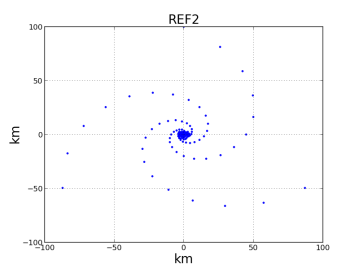
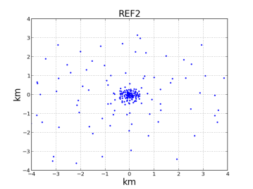
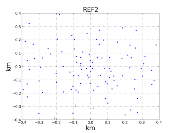
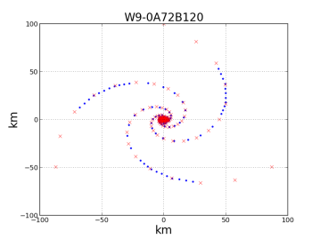
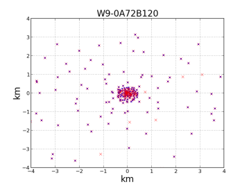
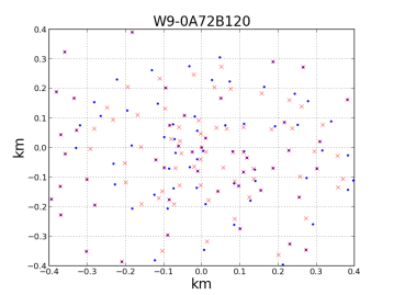
Figure 1: Antenna layouts on scales of $\pm$100 km (left), $\pm$4 km (centre) and $\pm$400 m (right). The REF2 layout is plotted on the upper row, and as red crosses for direct comparison to the W9-0A7B120 configuration on the lower row.

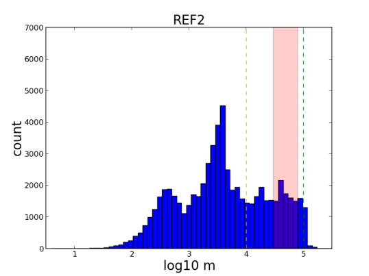
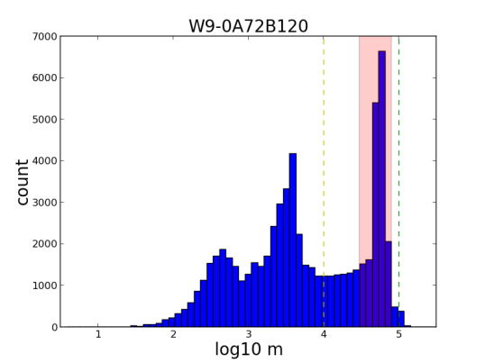
Figure 2: Baseline distribution with the uv-distance in log₁₀ km . Yellow and green dashed lines mark 10 and 120 kilometres respectively, and the pink strip represents baselines from 30-80 km.

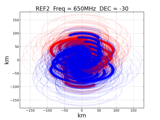
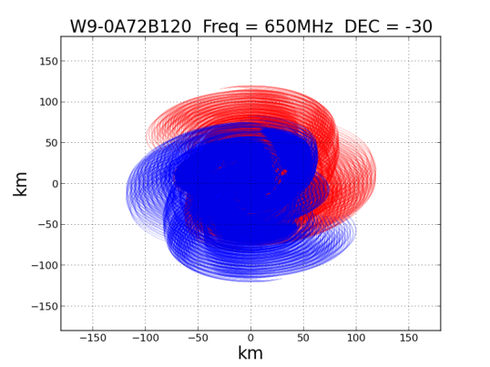
Figure 3: UV-Coverage for 8 hour tracks at 650 MHz (50 MHz wide channel) at declination -30 degrees for the different layouts. Blue indicates uv-points, red indicates conjugate uv-points.

The natural sensitivity at specific angular scales for an interferometer can be determined by making noise maps using only visibilities corresponding to those angular scales. Table 1 shows the sensitivity on angular scales {0.4-1, 1-2, 2-3, 3-4, 600-3600} arcsec for the two layouts under consideration. It is evident from this table that the W9-0A72B120 layout (henceforth, referred to as W9) has more sensitivity at small angular scales, but we note that further optimisations are still possible – even for different angular scales. In fact, the sophistication of simulation packages like MeqTrees (Noordam & Smirnov 2010) coupled with new insights into fundamental limits on radio interferometric imaging and calibration (Wijnholds & van der Veen 2008) allow for the distribution of array elements to be optimised subject to a well defined set of science of goals. It is also worth noting that the optimisation can be further constrained by cost and engineering limitations. Figure 4 shows the PSF sizes (uniform weighting) for the two layouts under consideration. The figure shows that the 120km W9 layout has very similar resolving performance compared to the 173km REF2.

	650MHz					800MHz					1000MHz
resbin	1	2	3	4	5	1	2	3	4	5	1	2	3	4	5
SKA1REF2	1.00	1.00	1.00	1.00	1.00	1.00	1.00	1.00	1.00	1.00	1.00	1.00	1.00	1.00	1.00
SKA1W9-0A72B120	0.77	0.81	1.12	1.06	1.00	0.72	1.05	1.06	1.17	1.06	0.72	1.05	1.08	1.26	1.05

(a)

Table 1: Relative (w.r.t REF2) RMS pixel noise for a 50MHz band after an 8hr synthesis with a 60s integration for the different layouts at different angular scales. These values are generated at 650, 800 and 1000 MHz, at angular scales {0.4-1, 1-2, 2-3, 3-4, 600-3600} arcsec and are labeled resbin {1, 2, 3, 4, 5} respectively. This is done for natural weighting at declination -30 degrees.

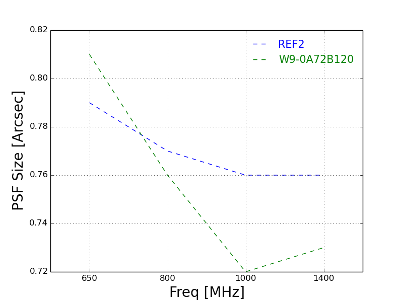
Figure 4: Uniformly weighted PSF sizes as a function of frequency for the REF2 (blue) and W9-0A72B120 (green) layouts.

3 The Experiment

Our aim is to gauge the sensitivity and resolution limits at which SKA1-MID can reliably detect and morphologically classify FRI, FRII and star forming galaxies (SFG). We note that we do not consider any evolution in the structure of the radio sources with redshift, or the effects of inverse Compton scattering, but note that such considerations would need quantifying in a more comprehensive study. We concentrate on SKA1-MID as it provides the best possibility of investigating source morphologies when compared to the very low resolution offered by SKA1-LOW and the factor of $\sim 2-3$ poorer resolution at a similar frequency for SKA1-SUR.

3.1 Telescope Simulations

We use the MAKEMS tool to make simulated measurement sets (MS) of 8 hour tracks centred at 700 MHz, with fifteen 50 MHz channels at a declination of -30 degrees. We then use the MeqTrees software to fill the MS with simulated visibilities. The noise per real and imaginary part for each visibility is calculated as

$$\sigma_{\text{vis}}=\text{SEFD}/\sqrt{2\Delta\nu\Delta t},$$ (1)

where $\Delta t$ is the integration time in seconds and $\Delta\nu$ is the channel width in Hertz. We use the baseline document’s system equivalent flux density (SEFD) value of 637 Jy for band 1. Note, the noise is proportional to the square-root of the synthesis time, therefore since we have “full” uv-coverage at 8 hours, we can reasonably approximate a $N$ hour synthesis for $N$ $>$ 8 by scaling the visibility noise as

$$\sigma_{\text{vis}}^{N}\simeq\sigma_{\text{vis}}\sqrt{8/N}.$$ (2)

We simulated a 10 hour synthesis using the REF2 and the alternative layout W9. The noise per visibility for both layouts is 8.69 mJy/beam, and the root mean square (RMS) of the pixel noise (uniform weighting) is $5.42~{}\mu$Jy/beam for REF2 and $5.29~{}\mu$Jy/beam for W9. Note that W9 is slightly more sensitive compared to REF2 due to the more complete uv-coverage over the scales of interest. Primary beam, calibration and atmospheric effects are beyond the scope of this chapter, however we note that significant progress has been (and continues to be) made in this area (see Smirnov, O. M. 2011; Grobler et al. 2014; Kazemi et al. 2011; Kazemi & Yatawatta 2013; Tasse, C. 2014).

3.2 Sky Models

Starting at redshift $z=1$, we use MeqTrees to predict visibilities for realistic flux distributions (FRI, FRII, or SFG galaxies) and use the LWIMAGER (part of the CASAREST package) tool to make clean maps. The clean maps are then processed (see Section 3.4) to determine the morphology of the flux distributions. This process is repeated at incrementally higher (steps of $z=0.5$) redshifts until detection or classification is no longer possible. For the FRI and FRII cases, we model a flat spectrum core with two hot-spots. The core has a luminosity of 7.94$\times 10^{22}$ WHz^-1sr^-1, with each hot-spot having 90% of the core luminosity and a spectral index of -0.7. The core and the hot-spots are modelled as point sources and the lobes as Gaussians. For convenience we consider the favourable inclination angle of 45 degrees. The true size of these sources is 200 kpc. For the SFG case we model a a Gaussian of luminosity 1.59$\times 10^{24}$ WHz^-1sr^-1 with a spectral index of -0.7, and a true size of 5 kpc.

3.3 Imaging Techniques

We make high resolution ($0.1^{\prime\prime}$) clean maps using Hogbom CLEAN (Högbom 1974); cleaning down to twice the rms pixel noise. Note that for uniform and Briggs weighting a crucial parameter is the size of the bin in the uv plane over which weights are “uniformised”. By default this is determined from the full image size, but LWIMAGER allows one to uniformise the weights over bins corresponding to a user-defined FoV instead. For these simulations uv-bins corresponding to a FoV of 10^′ were used.

3.4 Morphological Classification

The classification is done in two main steps: (i) locate bright compact emission and (ii) determine the extent of the lobes. For the former, we use the pyBDSM source finding tool. If there is one bright compact component the galaxy is classified as a SFG, while if more than one bright component is found the pixel statistics along the path joining the bright components are analysed in order to determine the extent of the lobes – see Figure 5 for an illustration. Finally, if lobes are detected, the galaxy can be classified as either FRI or FRII. This classification algorithm hinges on an accurate characterisation of the noise.

One crucial component in classifying these radio galaxies is an accurate characterisation of the jets, which is a major challenge at low SNR. This problem can be compounded by the inability to deconvolve the PSF at low SNR (this is particularly a problem for CLEAN). However a class of algorithms based on compressive sensing (CS) has recently emerged to tackle deconvolution issues in the context of the SKA and its precursor/pathfinder facilities (see section 4.4.2 in Norris et al. 2013), in particular MORESANE (Dabech et al. 2014, submitted) and PURIFY (Carrillo et al. 2014). Although not yet as well tested as CLEAN, these algorithms have been shown to be superior to CLEAN in detecting diffuse and compact emission, especially at low SNR(Ferrari et al. 2015, this volume). In addition to the CS-based algorithms, a Bayesian approach to radio interferometry imaging has led to the RESOLVE algorithm (Junklewitz et al. 2013), which has also been shown to produce better results compared to CLEAN. This progress in deconvolution algorithms will enhance the accuracy and depth of source characterisation algorithms.

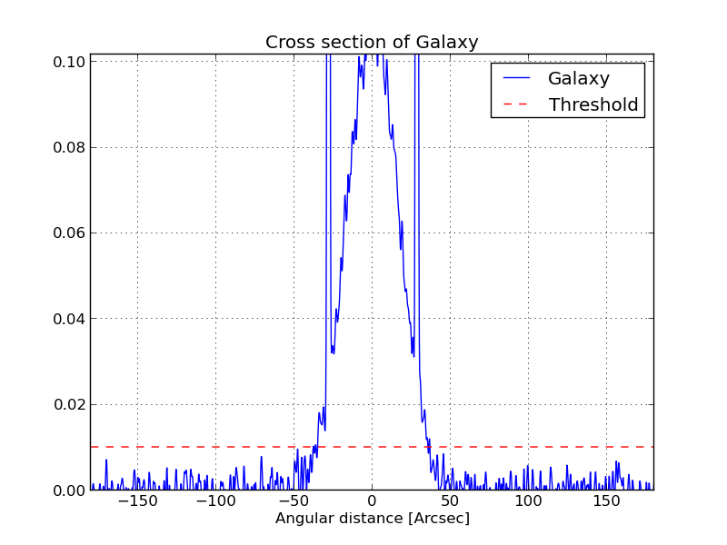
(a) High SNR, $z=4$

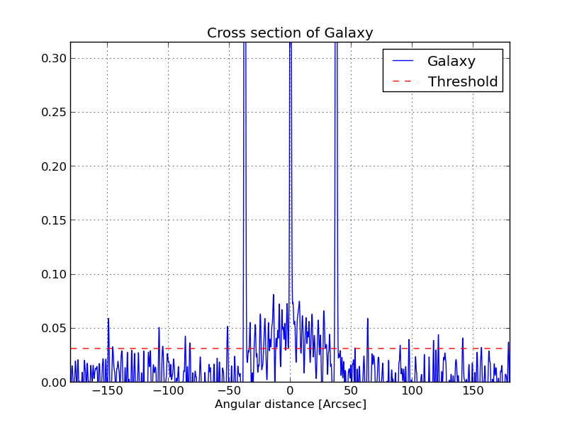
(b) Low SNR, $z=7$

Figure 5: Illustration of how the extent of the lobes is determined for an FR2 source. In both cases, having found the hot spots, the RMS of pixels within some box ($20\times 20$ pixels in this case) along the path connecting the hot spots is computed. If the RMS is above some threshold (red line), then the pixels are taken to be part of the lobes. Finally, the edges of the lobes can be determined by keeping track of where the RMS of the pixels within this box gets larger than the threshold.

4 Simulation Results

Before we present the simulations results, we first show in Figure 6 how the SNR varies with redshift assuming the sky models and the observation set up described in Section 3. From these figures it is clear that SKA1-MID will be able to probe radio emission at very high redshifts. For FR sources we expect an SNR (w.r.t the lobe surface brightness for FR sources) of 3 at redshifts around 5.5, and the same SNR at a redshift of 5 for SFGs after 10 hours of integration and after 100 hours of integration we expect an SNR of 3 at redshifts of 9.5 for FR sources and 8.5 for SFGs. On the other hand, morphological characterisation will be limited by the ability to resolve these sources. SKA1-MID with a $\sim 0.5^{\prime\prime}$ PSF (uniform weighting) at 700 MHz, will not be able to resolve sources of sizes less than 5 kpc (see Figure 7).

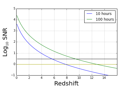
(a) FRI and FRII sources

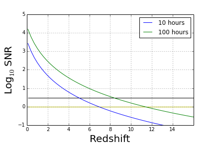
(b) SFGs

Figure 6: The SNR (relative to the surface brightness) from a 10 (blue) and a 100 (green) hour synthesis as a function of redshift for FRI and FRII sources (left) and the SFGs (right). Lines of constant SNR=1 (yellow) and SNR=3 (black) also plotted. These plots were generated using the REF2 layout.

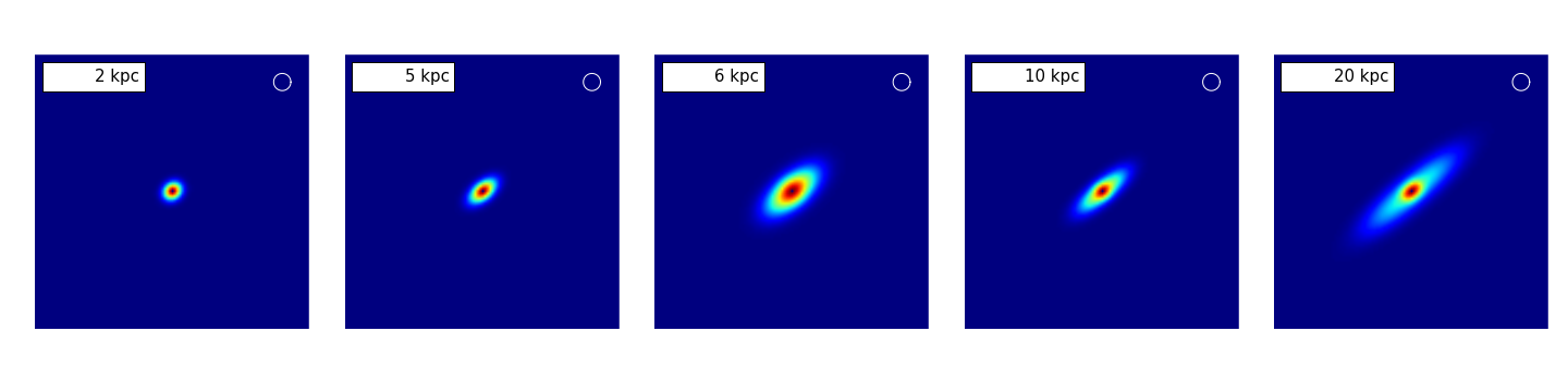
(a)

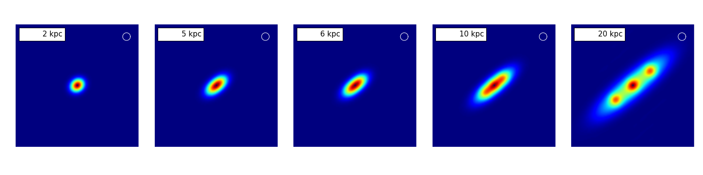
(b)

Figure 7: Model FR1 (row 1) and FR2 (row 2) sources of different sizes as seen by the REF2 layout at $z=1$. The white circle on the top left corner gives an indication the PSF size (0.51^′′).

In Figures 8-10 we show images of the galaxies under consideration as a function of redshift. For each galaxy type we show the sky model (row 1) and images from simulations using the REF2 and W9 layouts (rows 2 and 3 respectively). Our morphological classification algorithm was able to detect and distinguish FR sources up to a redshift of 8, and up to a redshift of 5 for the SFGs after 10 hours of integration. Note that in the SFG case, we set a 5$\sigma$ threshold for the pyBDSM source finder to avoid false detections, however detection and classification of these sources can (potentially) still be done below the 5$\sigma$ level if the false detections can be quantified using techniques such as described in Serra et al. (2012).

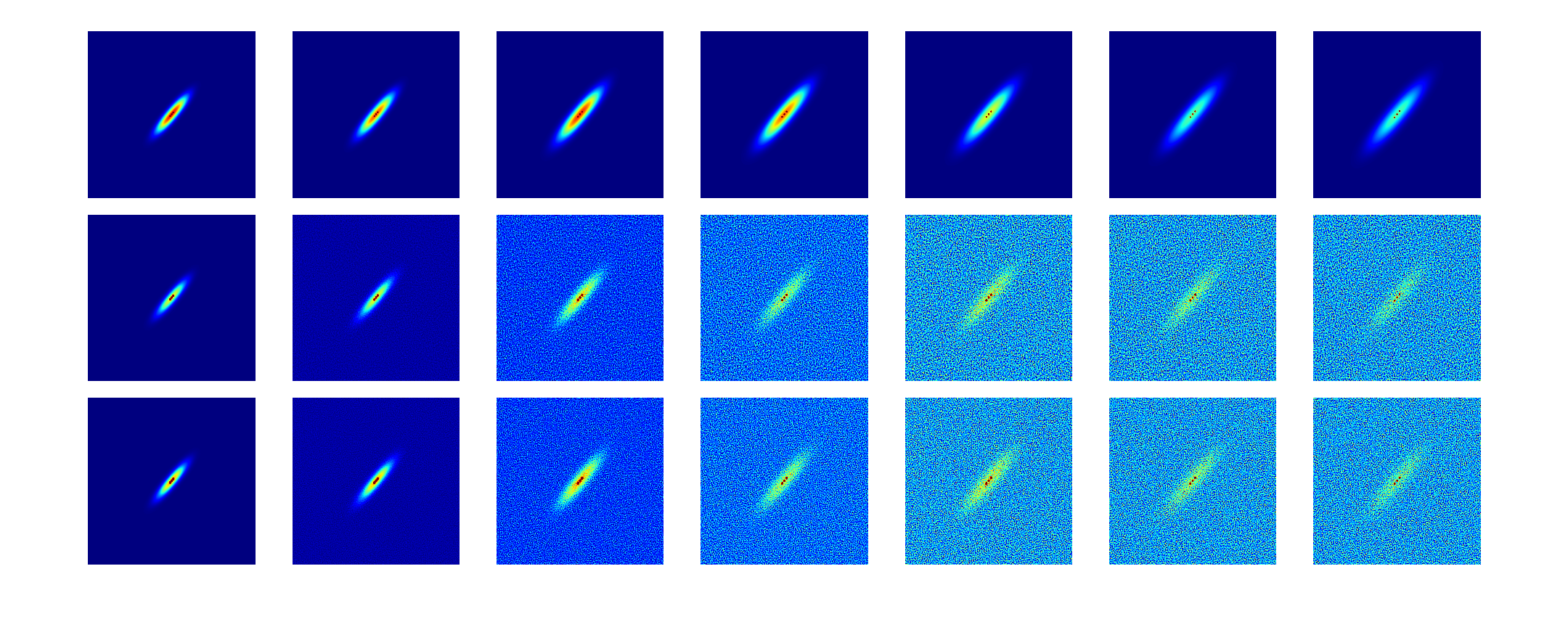
Figure 8: Model FRI galaxies (row 1) as a function of redshift {1, 2, 3, 4, 5, 6, 7, 7.5, 8, 8.5} as seen by the REF2 (row 2) and W9 (row 3) layouts after a 10 hour synthesis.

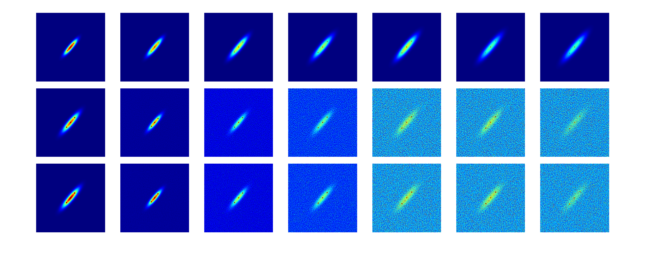
Figure 9: Model FRII galaxies (row 1) as a function of redshift {1, 2, 3, 4, 5, 6, 7, 7.5, 8, 8.5} as seen by the REF2 (row 2) and W9 (row 3) layouts after a 10 hour synthesis.

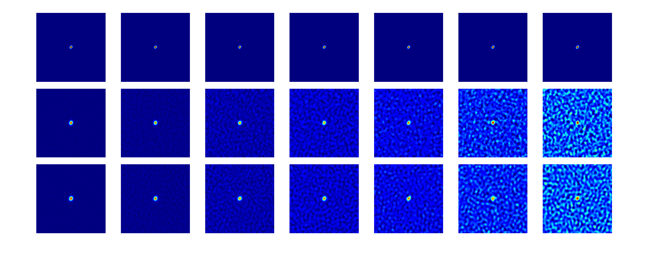
Figure 10: Model SF galaxies (row 1) as a function of redshift {1, 2, 3, 3.5, 4, 4.5, 5} as seen by the REF2 (row 2) and W9 (row 3) layouts after a 10 hour synthesis.

Now we consider three cases along the timeline that SKA1 may be built out: (i) a 50% SKA1-MID sensitivity, (ii) a 70% SKA1-MID in terms of sensitivity, and (iii) is the full SKA facility– with 10 times the sensitivity of SKA1-MID. Figure 11 shows how the SNR from a 10 hour synthesis varies with redshift for these three cases.

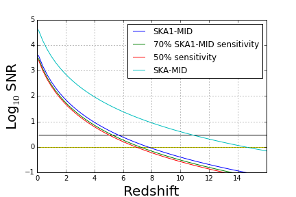
(a) FRI and FRII sources

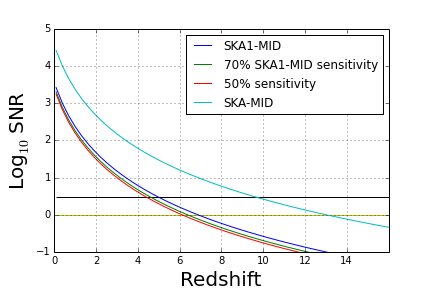
(b) SFGs

Figure 11: The SNR (relative to the surface brightness) from a 10 hour synthesis as a function of redshift for FRI and FRII sources (left) and the SFGs (right). The plots are for 4 cases: (i) SKA1-MID sensitivity (blue), (ii) 70% SKA1-MID sensitivity (green), (iii) 50% SKA1-MID (red) and (iv) full SKA-MID sensitivity (sky blue; assuming SKA-MID has 10 times the sensitivity of SKA1-MID). Lines of constant SNR=1 (yellow) and SNR=3 (black) are also plotted.

5 Conclusions

Our simulation results suggest that accurate morphological classification of these high redshift radio sources will be feasible even at the most extreme redshifts (up to $z\sim 8$ after 10 hours integration) in deep SKA1-MID images. These results also show that (at least for the case we have considered) an SKA1-MID layout with a maximum baseline length of 120 km does as well as the second generation baseline layout which has a maximum baseline length of around 170 km. In fact, the W9 layout is slightly more sensitive to our simulated galaxies as can seen in Figures 8 and 9. This would mean that for science cases where it is important to morphologically classify radio sources, e.g. for galaxy evolution (see Ferramacho et al. 2014; Camera et al. 2015, this volume) the proposed 120 km layout has an advantage, and longer baselines are not necessary.

Morphological classification will be limited by resolution and not sensitivity. SKA1-MID will be able to resolve radio sources down to scales of $\sim 5$ kpc at cosmological distances. Morphological classification at smaller scales will require higher resolution. This is only available by going to higher frequencies (though impractical in a survey scenario due to the reduced field of view), or with substantially longer baselines, such as those provided by the full SKA dish array with stations in SKA partner countries.

It is also worth noting that model fitting techniques (Martí-Vidal et al. 2014; White et al. 1997; Reid 2006) have the capability to “super-resolve” multiple components within the PSF main lobe. Given the high sensitivity of SKA1-MID, the prospects of morphologically separating star formation and AGN activity are very good since the ability to infer the morphology of sub-resolution sources scales as $\sqrt{SNR}$ (Martí-Vidal et al. 2014). In particular, with SKA1-MID achieving an SNR of 10 to 100 in the range z=$1\sim 4$, this translates into the ability to resolve features of roughly one third to a 10th of the PSF size via model fitting, thus making morphological classification of kpc-scale sources possible.

A more general algorithm (compared to the one presented here) will be required to do this classification in deep field images with multiple sources. Such algorithms can be further improved by considering spectral and polarization information.