Star formation in turbulent molecular clouds with colliding flow

Abstract

Using self-gravitational hydrodynamical numerical simulations, we investigated the evolution of high-density turbulent molecular clouds swept by a colliding flow. The interaction of shock waves due to turbulence produces networks of thin filamentary clouds with a sub-parsec width. The colliding flow accumulates the filamentary clouds into a sheet cloud and promotes active star formation for initially high-density clouds. Clouds with a colliding flow exhibit a finer filamentary network than clouds without a colliding flow. The probability distribution functions (PDFs) for the density and column density can be fitted by lognormal functions for clouds without colliding flow. When the initial turbulence is weak, the column density PDF has a power-law wing at high column densities. The colliding flow considerably deforms the PDF, such that the PDF exhibits a double peak. The stellar mass distributions reproduced here are consistent with the classical initial mass function with a power-law index of $-1.35$ when the initial clouds have a high density. The distribution of stellar velocities agrees with the gas velocity distribution, which can be fitted by Gaussian functions for clouds without colliding flow. For clouds with colliding flow, the velocity dispersion of gas tends to be larger than the stellar velocity dispersion. The signatures of colliding flows and turbulence appear in channel maps reconstructed from the simulation data. Clouds without colliding flow exhibit a cloud-scale velocity shear due to the turbulence. In contrast, clouds with colliding flow show a prominent anti-correlated distribution of thin filaments between the different velocity channels, suggesting collisions between the filamentary clouds.

1. Introduction

Turbulence of the interstellar medium plays an important role in star formation (Elmegreen & Scalo, 2004; Scalo & Elmegreen, 2004; McKee & Ostriker, 2007). It is widely accepted that turbulence controls the fragmentation of molecular clouds. When the fragments are gravitationally unstable, dense fragments caused by strong shocks undergo collapse to form stars (e.g., Klessen et al., 2000). Consequently, characteristics of star formation, such as star-formation rates and star-formation efficiency, are presumed to be affected by turbulence (Krumholz & McKee, 2005; Padoan & Nordlund, 2011; Hennebelle & Chabrier, 2011).

In addition to turbulence, molecular clouds are affected by external effects. It has been thought that H ii regions and stellar winds from OB stars trigger star formation in associated molecular clouds (Elmegreen & Lada, 1977). For example, supernova remnants interact with the interstellar medium (McKee & Ostriker, 1977). Observations suggest that supernova remnants also trigger star formation (e.g., Koo et al., 2008; Gouliermis et al., 2008), although this manner of formation is still under debate (Desai et al., 2010).

Theoretically, Hartmann et al. (2001) proposed a scenario of dynamical star formation, where large-scale flow in the interstellar medium accumulates gas to promote rapid star formation. Vázquez-Semadeni et al. (2007), Banerjee et al. (2009), and Gómez & Vázquez-Semadeni (2014) examined the formation of giant molecular clouds and stars within them by considering the collision of a warm neutral medium. Gong & Ostriker (2011) and Chen & Ostriker (2014) considered cloud core formation in turbulent clouds with supersonic converging flows, by using hydrodynamical and ambipolar-diffusion magnetohydrodynamics (MHD) simulations. These theoretical studies indicate that both the external flow and the turbulence are important factors influencing cloud core formation and star formation.

Recently, Dobashi et al. (2014) carried out molecular line observations of the massive dense cloud L1004E, which is located in the Cyg OB 7 giant molecular cloud. The characteristic features of L1004E are a high mass of $\sim 10^{4}\,M_{\sun}$ within a small region $\sim(5~{}\mathrm{pc})^{2}$, a low temperature of $\sim 9$ K, and a broad line width of $\sim 2\,\mathrm{km\,s}^{-1}$ corresponding to Mach 10 turbulence. A small number of protostar candidates associated with the cloud suggests that the cloud is probably in a stage prior to active star formation or has just begun forming stars. Moreover, their observations suggest a dynamical process inside L1004E, where several filamentary clouds can be identified as internal structures that interact with each other by collisions. The interaction may induce star formation. They also suggested that the interaction between filaments is caused by compression due to an external effect, e.g., the shock of nearby supernova remnants.

Recent observations indicate that filaments are the basic unit of structure in molecular clouds. Observations by the Herschel survey revealed networks of parsec-scale filaments in many clouds (e.g., André et al., 2010; Men’shchikov et al., 2010; Arzoumanian et al., 2011). Hacar et al. (2013) showed that filamentary cloud L1495/B213 in the Taurus region has a substructure containing many filaments. Nakamura et al. (2014) suggested that the collisions of filaments may have triggered cluster formation.

Motivated by the observations of Dobashi et al. (2014) and taking into account compression on a cloud scale, we performed numerical simulations of self-gravitational turbulent molecular clouds. Although self-gravitational turbulent gas has been investigated by many authors (e.g. Klessen et al., 2000; Ostriker et al., 2001; Heitsch et al., 2001; Federrath et al., 2008; Nakamura & Li, 2008; Offner et al., 2008; Padoan & Nordlund, 2011), simulations are still limited for clouds with strong turbulence and low temperature, such as L1004E (Padoan & Nordlund, 2011). Moreover, the influence of cloud-scale compression on star formation in these clouds is poorly understood.

This paper is organized as follows. In Section 2 and Section 3, the model and simulation methods are presented. The results of the simulations are shown in Section 4, and they are discussed in Section 5. Finally, conclusions of this paper are given in Section 6.

2. Models of Turbulent Clouds

As the initial condition, we consider clouds with a constant density and turbulent velocity. The clouds are swept by head-on colliding flows. The initial models are classified according to the initial density $\rho_{0}$, the initial Mach number of turbulence ${\cal M}_{t}$, and the Mach number for a colliding flow ${\cal M}_{f}$. The model parameters are summarized in Table 1.

Table 1Model parameters

Model	$\rho_{0}$	$n_{0}$	$M_{\mathrm{tot}}$	${\cal M}_{t}$	${\cal M}_{f}$	$t_{\mathrm{ff}}/t_{\mathrm{cross}}$	$N_{\star}$	$t_{10M_{\sun}}$
	($10^{-21}\mathrm{g}\,\mathrm{cm}^{-3}$)	($10^{3}\mathrm{cm}^{-3}$)	($10^{3}M_{\sun}$)					($10^{6}$ yr)
HT3F0	5.42	1.420	10.0	3	0	0.11	135 (13)	1.43
HT10F0	5.42	1.420	10.0	10	0	0.35	140 (12)	0.87
HT30F0	5.42	1.420	10.0	30	0	1.06	265 (19)	0.76
HT10F3	5.42	1.420	10.0	10	3	0.36	260 (15)	0.87
HT10F10	5.42	1.420	10.0	10	10	0.43	142 (11)	0.56
HT10F30	5.42	1.420	10.0	10	30	0.83	915 (54)	0.50
LT3F0	1.00	0.262	1.85	3	0	0.25	14 0(0)	3.16
LT10F0	1.00	0.262	1.85	10	0	0.82	9 0(0)	2.51
LT30F0	1.00	0.262	1.85	30	0	2.46	3 0(1)	2.21
LT10F3	1.00	0.262	1.85	10	3	0.84	25 0(0)	2.08
LT10F10	1.00	0.262	1.85	10	10	1.00	25 0(0)	1.55
LT10F30	1.00	0.262	1.85	10	30	1.92	55 (34)	1.27
HT10F0wog	5.42	1.420	10.0	10	0	$\cdots$	$\cdots$	$\cdots$
HT10F10wog	5.42	1.420	10.0	10	10	$\cdots$	$\cdots$	$\cdots$

The constant initial density is assumed to be $\rho_{0}=5.42\times 10^{-21}\,\mathrm{g}\,\mathrm{cm}^{-3}$ (corresponding to the number density $n_{0}=1.42\times 10^{3}\,\mathrm{cm}^{-3}$) for high-density models, and $\rho_{0}=10^{-21}\,\mathrm{g}\,\mathrm{cm}^{-3}$ ($n_{0}=2.62\times 10^{2}\,\mathrm{cm}^{-3}$) for low-density models. The computational domain is a cubic box with sides $L=5~{}\mathrm{pc}$, and the total masses of gas are therefore $M_{\mathrm{tot}}=1.00\times 10^{4}\,M_{\odot}$ for the high-density models and $M_{\mathrm{tot}}=1.85\times 10^{3}\,M_{\odot}$ for the low-density models. The mass of the high-density models mimics the high-mass core L1004E in the Cyg OB 7 molecular cloud (Dobashi et al., 2014).

The gas is assumed to be isothermal with a temperature of 10 K, and the corresponding sound speed is $c_{s}=0.19\,\mathrm{km}\,\mathrm{s}^{-1}$. This temperature is in agreement with that in L1004E, which is estimated as $8~{}\mathrm{K}\lesssim T\lesssim 12~{}\mathrm{K}$ with a mean value of $\sim 9$ K (Dobashi et al., 2014). The initial Jeans length is defined by $\lambda_{J}=(\pi c_{s}^{2}/G\rho_{0})^{1/2}$, and it is evaluated as 0.57 pc and 1.33 pc for the high-density and low-density models, respectively. The ratio of the size of the computational domains to the Jeans length is $L/\lambda_{J}=8.7$ and 3.7 for the high-density and low-density models, respectively. Therefore, the total masses in units of the Jeans mass for the high-density models and low-density models are $M_{\mathrm{tot}}/M_{J}=6.59\times 10^{2}$ and $5.23\times 10^{1}$, respectively, where the Jeans mass is defined by $M_{J}=\rho_{0}\lambda_{J}^{3}$. The freefall times are $t_{\mathrm{ff}}=9.05\times 10^{5}$ yr and $2.11\times 10^{6}$ yr, respectively, for the high-density and low-density models, where the freefall time is defined by $t_{\mathrm{ff}}=(3\pi/32G\rho_{0})^{1/2}$. The magnetic field is ignored in this paper for simplicity.

A turbulent velocity is imposed on the initial stage and decay of the turbulence follows, under the consideration of no driving force for turbulence (see for detail Matsumoto & Hanawa, 2011). The initial velocity field is solenoidal with a power spectrum of $P(k)\propto k^{-4}$, generated according to Dubinski et al. (1995), where $k$ is the wavenumber. This power spectrum results in a velocity dispersion of $\sigma_{v}(\lambda)\propto\lambda^{1/2}$, where $\lambda$ is the scale length, which is in agreement with the Larson scaling relations (Larson, 1981). Note that the kinetic energy of the turbulence is given by $E_{K}=\int P(k)4\pi k^{2}dk$ in our definition. An alternative definition of the power spectrum is $E(k)=4\pi k^{2}P(k)$, and the kinetic energy is given by $E_{K}=\int E(k)dk$, yielding the relationship $E(k)\propto k^{-2}$. The models are constructed by changing the root mean square (rms) Mach number of the initial velocity field in the range ${\cal M}_{t}=3-30$. The rms Mach number is defined by

$${\cal M}_{t}=\left[\frac{1}{c_{s}^{2}L^{3}}\int_{V}\left|\mbox{\boldmath$v$}_{t}^{2}\right|dV\right]^{1/2},$$ (1)

where $\mbox{\boldmath$v$}_{t}$ denotes the turbulent velocity and $\int_{V}dV$ denotes the volume integration over the computational domain. We utilize a common velocity pattern as the template for producing the initial turbulence among all models.

To investigate the effects of a colliding gas flow, a large-scale sinusoidal flow is also imposed on the initial stage as

$$\mbox{\boldmath$v$}_{f}=\left(\begin{array}[]{c}\displaystyle{\cal M}_{f}c_{s}\sin\frac{2\pi x}{L}\\ 0\\ 0\end{array}\right),$$ (2)

where ${\cal M}_{f}$ denotes the amplitude of the flow in units of Mach number, and it changes in the range of ${\cal M}_{f}=0-30$ for constructing the models. Due to this flow, turbulent gas converges to the $x=0$ plane. This flow mimics the effects of the external environment, e.g., shock fronts of supernova remnants, H ii regions, or stellar winds from nearby OB stars.

By using the two Mach numbers ${\cal M}_{t}$ and ${\cal M}_{f}$, the effective Mach number for the flows is defined by ${\cal M}_{\mathrm{eff}}=({\cal M}_{t}^{2}+{\cal M}^{2}_{f}/2)^{1/2}$. The factor $1/2$ for ${\cal M}_{f}^{2}$ comes from the average of the sinusoidal flow $\mbox{\boldmath$v$}_{f}$ over the computational domain. The crossing time is then evaluated as $t_{\mathrm{cross}}=L/({\cal M}_{\mathrm{eff}}c_{s})=2.57\times 10^{6}\left({\cal M}_{\mathrm{eff}}/10\right)^{-1}\,\mathrm{yr}$.

As summarized in Table 1, we call these models HT10F0, LT3F0, etc. The model names are constructed as follows. The 1st character, “H” or “L”, corresponds to the high-density or low-density models, respectively. The digits following “T”, which is the turbulence, denote the initial Mach number for the turbulence, ${\cal M}_{t}$. The digits following “F”, which is the flow, denote the initial Mach number for the colliding flow, ${\cal M}_{f}$.

We also calculated models HT10F0 and HT10F10 without considering self-gravity. These models are referred to as “HT10F0wog” and “HT10F0wog”, and are calculated for the long time of $t\simeq 2.5\times 10^{7}\,\mathrm{yr}\simeq 10t_{\mathrm{cross}}$. The turbulence decays, reducing the velocity dispersion to $\simeq 7.9\%$ and 6.6% of the initial value for models HT10F0wog and HT10F10wog, respectively.

Note that the models presented here can be scaled to different sizes because the gas is assumed to be isothermal. The size of the problem is specified by the non-dimensional parameter $L/\lambda_{J}$, or equivalently $M_{\mathrm{tot}}/M_{J}$, or $t_{\mathrm{ff}}/t_{\mathrm{sc}}$, where $t_{\mathrm{sc}}(=L/c_{s}=2.6\times 10^{7}\,\mathrm{yr)}$ denotes the sound crossing time.

3. Numerical Methods

We calculated the evolution of a cloud by the numerical simulation code, SFUMATO (Matsumoto, 2007). The total variation diminishing (TVD) cell-centered scheme is adopted as the hydrodynamical solver. The hydrodynamical solver achieves second-order accuracy in space and time. The self-gravity is solved by the multigrid method, which exhibits spatial second-order accuracy. The numerical fluxes are conserved by using the refluxing procedure in both the hydrodynamics and the self-gravity solvers. The periodic boundary condition is imposed for the hydrodynamics and the self-gravity.

SFUMATO utilizes a block-structured adaptive mesh refinement (AMR) technique. The computational domain of $(5~{}\mathrm{pc})^{3}$ is resolved by a uniform grid having $512^{3}$ cells for the high-density models and $256^{3}$ cells for the low-density models at the initial stage. The initial resolutions are therefore $\Delta x=1.0\times 10^{-2}\,\mathrm{pc}$ for the high-density models and $\Delta x=2.0\times 10^{-2}\,\mathrm{pc}$ for the low-density models. The Jeans condition is employed as a refinement criterion. Blocks are refined when the Jeans length is shorter than 8 times the cell width: $(\pi c_{s}^{2}/G\rho)^{1/2}<8\Delta x$ (see Truelove et al., 1997). The finest resolution is set at $\Delta x_{\mathrm{min}}=5.0\times 10^{-3}\,\mathrm{pc}$ for both the high-density and low-density models, and the effective mesh size is therefore $1024^{3}$. This mesh size is the same as that of the recent high-resolution simulations (e.g., Federrath et al., 2010b).

Sink particles are implemented to reproduce star formation in the model clouds. Sink particles are Lagrangian particles moving on the numerical grid and interacting with the gas through gravity and accretion. The threshold density for particle creation is set at $\rho_{\mathrm{sink}}=1.17\times 10^{-18}\,\mathrm{g}\,\mathrm{cm}^{-3}$ (corresponding number density is $3.07\times 10^{5}\,\mathrm{cm}^{-3}$). Fragmentation during gravitational collapse in a very high density regime ($\rho>\rho_{\mathrm{sink}}$) does not occur, and the number of sink particles exhibited in the simulations is therefore the lower limit of the number of stars produced in the clouds. Sink particles accrete gas located within a radius $r_{\mathrm{sink}}=1.95\times 10^{-2}\,\mathrm{pc}$, which is equal to $4\Delta x_{\mathrm{min}}$ as well as half of the Jeans length for $\rho_{\mathrm{sink}}$. The details of the method for sink particles are shown in Appendix A.

We followed the evolution of the clouds until the stage in which the maximum mass of sink particles exceeds $10\,M_{\sun}$. Further evolution is beyond the scope of this paper because no feedback from star formation is considered in the simulations.

4. Results

4.1. Fiducial model with high density HT10F0

The evolution of the high-density model with ${\cal M}_{t}=10$ and ${\cal M}_{f}=0$ is described here as a fiducial model without the colliding flow. Figure 1 shows the evolution of model HT10F0 by the distributions of column density and sink particles. In the early phase, turbulence produces many shock waves, as shown in Figure 1(a). The density, which increases by a factor of $\sim 10^{2}$ due to shock compression, indicates that the density contrast of the isothermal shock is equal to the square of the Mach number. The first star forms at $t=5.65\times 10^{5}\,\mathrm{yr}$, which corresponds $0.22t_{\mathrm{cross}}$ and $0.62t_{\mathrm{ff}}$, as shown in Figure 1(b). Sink particle formation earlier than the freefall time is the result of the density increase due to the shock waves. At this stage, models HT10F0 and HT10F0wog show similar density distributions, which indicates that turbulence mainly controls the structure formation. Figure 1(c) shows the cloud at the stage where the maximum mass of sink particles reaches $10\,M_{\sun}$ (hereafter referred to as “the stage of $M_{\mathrm{\star,max}}=10\,M_{\sun}$”). By this stage, the density contrast increases more than that shown in Figure 1(b), and it is slightly higher than that of model HT10F0wog because of self-gravity. Sink particles are created in clusters along the dense filaments.

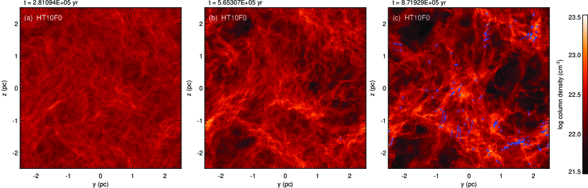
Figure 1.— Evolution of model HT10F0 at three representative stages: (a) the early stage, (b) the stage of the first star formation, and (c) the stage of $M_{\mathrm{\star,max}}=10M_{\sun}$. The color scale shows the column density in the $x$-direction. The blue circles and their associated lines show the positions of sink particles and their loci, respectively.

4.2. Dependence on the initial strength of the turbulence

Figure 2 shows the dependence of the high-density models (upper panels) and low-density models (lower panels) without colliding flow (${\cal M}_{f}=0$) on the initial strengths of the turbulence.

The stronger turbulent models produce a fine structure of gas, whereas the weak turbulent models show parsec-scale filaments irrespective of the initial densities. Model HT30F0 exhibits small structures disturbed by strong turbulence, whereas model HT3F0 exhibits a network with long filaments. Similarly, model LT3F0 shows smoother filaments than does LT30F0.

For the high-density models, a model with stronger turbulence produces more sink particles in a shorter time (see also Table 1). This is attributed to strong compression due to a large amount of turbulence, as shown in the previous work of Klessen et al. (2000). The long loci of sink particles in the more turbulent model, HT30F0, indicate the high speeds of the sink particles. These sink particles move at velocities roughly similar to those of the gas where they formed. Details of the velocity distribution for sink particles are shown in Section 4.9.

The low-density models produce much smaller numbers of sink particles compared to the high-density models (see also Table 1). This indicates that the high-density models contain larger masses than the low-density models. Contrary to the high-density models, a model with stronger turbulence produces fewer sink particles by the stage of $M_{\mathrm{\star,max}}=10\,M_{\sun}$, as shown in the lower panels of Figure 2 and Table 1. However, at a given time, a model with stronger turbulence produces more sink particles, showing that the turbulence promotes star formation even for the low-density models.

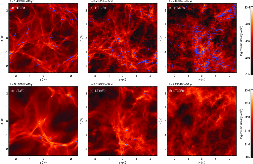
Figure 2.— Comparison of clouds in models with different strengths of initial turbulence and without the colliding flow (${\cal M}_{f}=0$) at the stages of $M_{\mathrm{\star,max}}=10M_{\sun}$. The upper and lower figures show the high-density models and the low-density models, respectively. The left, middle, and right figures show the models with ${\cal M}_{t}=3,10,$ and 30, respectively. The color scale shows the column density in the $x$-direction. The blue circles and their associated lines show the positions of the sink particles and their loci, respectively.

4.3. Model with colliding flow HT10F10

Model HT10F10 is the same as the previous model, HT10F0, but colliding flow with a Mach number of 10 is added. Figure 3 shows the evolution of model HT10F10. The upper and lower panels show the column densities along the $x$- and $z$-directions, respectively. Figures 3(a) and 3(d) show the cloud in the early phase. The column density along the $x$-direction (Figure 3(a)) is similar to that of model HT10F0 (Figure 1(a)), and the gas compression due to the colliding flow is shown in the column density along the $z$-direction (Figure 3(d)). Figures 3(b) and 3(e) show the cloud when the first sink particle forms. The colliding flow accumulates filaments to form a sheet at $x\simeq 0$, and the dense gas of the sheet leads to star formation at an earlier time than for the previous model.

Figures 3(c) and 3(f) show the cloud at the stage of $M_{\mathrm{\star,max}}=10\,M_{\sun}$. The thickness of the sheet increases because the accumulated filaments penetrate the sheet. In the comparison of Figure 1(c) and Figure 3(c), model HT10F10 exhibits more prominent fine filaments. The filamentary structure is enhanced by the self-gravity, while the structure formation is primarily dominated by the turbulence. The colliding flow increases the density in the sheet, increasing the effects of the self-gravity. We confirmed that the dense filaments with widths of $\sim 0.1$ pc have the Jeans length less than $0.1$ pc, indicating that the self-gravity also contributes to the structure formation mainly on a scale of the filament width. The number of sink particles is roughly the same as that of model HT10F0 (Table 1), but the elapsed time is shorter than that in model HT10F0 due to the high accretion rate, which indicates that the colliding flow promotes star formation.

The column density along the $z$-direction shows that dense filaments lie parallel to the sheet and low-density striations lie perpendicular to the sheet. The low-density striations are oriented parallel to the accretion flow on the sheet. The column density and the velocity are in agreement with recent observations of Palmeirim et al. (2013). After finding striations perpendicular to the filament in the B211/L1495 region in the Taurus molecular cloud , they suggest that gas may be accreting along the striations onto the main filament.

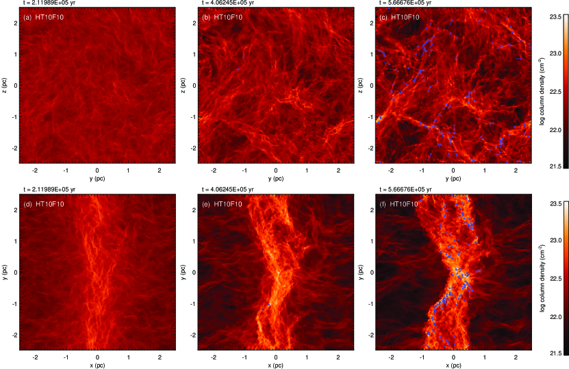
Figure 3.— Evolution of model HT10F10 at three representative stages: (a, d) the early stage, (b, e) the stage of the first star formation, and (c, f) the stage of $M_{\mathrm{\star,max}}=10M_{\sun}$. The color scale shows the column density in the $x$-direction (upper figures) and the $z$-direction (lower figures). The blue circles and their associated lines show the positions of the sink particles and their loci, respectively.

4.4. Dependence on the colliding flow

Figure 4 shows the high-density models with different strengths of colliding flows in column densities along the $x$-direction (upper panels) and the $z$-direction (lower panels). The model with a strong flow, HT10F30, exhibits strong compression of gas into the plane at $x\simeq 0$, as shown in the column densities along the $z$-direction. This leads to fine filaments and active formation of sink particles compared to the previous model, HT10F10, as shown in the column densities along the $x$-direction. Model HT10F10 produces 142 sink particles, while model HT10F30 produces 915 sink particles.

The model with weak colliding flow, HT10F3, does not exhibit a clear sheet structure at $x\simeq 0$, as shown in Figure 4(d). This is because the amplitude of the colliding flow is considerably lower than the mean velocity of the initial turbulence (${\cal M}_{f}<{\cal M}_{t}$). The low compression due to the colliding flow leads to a long elapsed time for the maximum mass of the sink particles to reach $10\,M_{\sun}$. This long time brings about formation of many sink particles compared to the case for model HT10F10.

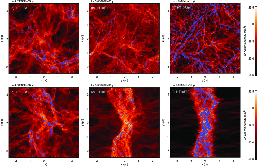
Figure 4.— Comparison between the high-density models with a common initial turbulence of ${\cal M}_{t}=10$ and with different strengths of colliding flows at the stages of $M_{\mathrm{\star,max}}=10M_{\sun}$. The left, middle, and right figures show models with ${\cal M}_{f}=3,10,$ and 30, respectively. The color scale shows the column density in the $x$-direction (upper figures) and the $z$-direction (lower figures). The blue circles and their associated lines show the positions of the sink particles and their loci, respectively.

Figure 5 compares the low-density models with different strengths of colliding flows. In the low-density models, formation of sink particles begins after the colliding flows pass by each other. At the stage of $M_{\mathrm{\star,max}}=10\,M_{\sun}$, the sheet structures due to colliding flows disappear.

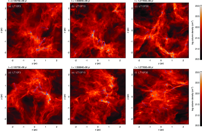
Figure 5.— Comparison between the low-density models with a common initial turbulence of ${\cal M}_{t}=10$ and with different strengths of colliding flows at the stage of $M_{\mathrm{\star,max}}=10M_{\sun}$. The left, middle, and right figures show models with ${\cal M}_{f}=3,10,$ and 30, respectively. The color scale shows the column density in the $x$-direction (upper figures) and the $z$-direction (lower figures). The blue circles and their associated lines show the positions of the sink particles and their loci, respectively.

4.5. Decay of turbulence

Figure 6 shows the decay of turbulence by measuring the standard deviations of the velocities (velocity dispersion), $\sigma_{v}=\langle(\mbox{\boldmath$v$}-\langle\mbox{\boldmath$v$}\rangle_{m})^{2}\rangle_{m}^{1/2}$, where $\langle\cdot\rangle_{m}$ denotes the mass-weighted average over the computational domain, i.e., $\langle\mbox{\boldmath$v$}\rangle_{m}=\int_{V}\rho\mbox{\boldmath$v$}\,dV/M_{\mathrm{gas,tot}}$ and $M_{\mathrm{gas,tot}}=\int_{V}\rho dV$. The total kinetic energy of gas is therefore evaluated as $E_{K}=M_{\mathrm{gas,tot}}\sigma_{v}^{2}/2$ when $\langle\mbox{\boldmath$v$}\rangle_{m}=0$. Our numerical scheme conserves the linear momentum of gas within a truncation error before sink particle formation, and the mean velocity $\langle\mbox{\boldmath$v$}\rangle_{m}$ therefore has small values compared to $\sigma_{v}$. Even after sink particle formation, the mean velocity remains small, $\langle\mbox{\boldmath$v$}\rangle_{m}/\sigma_{v}\lesssim 10^{-3}-10^{-2}$ at most.

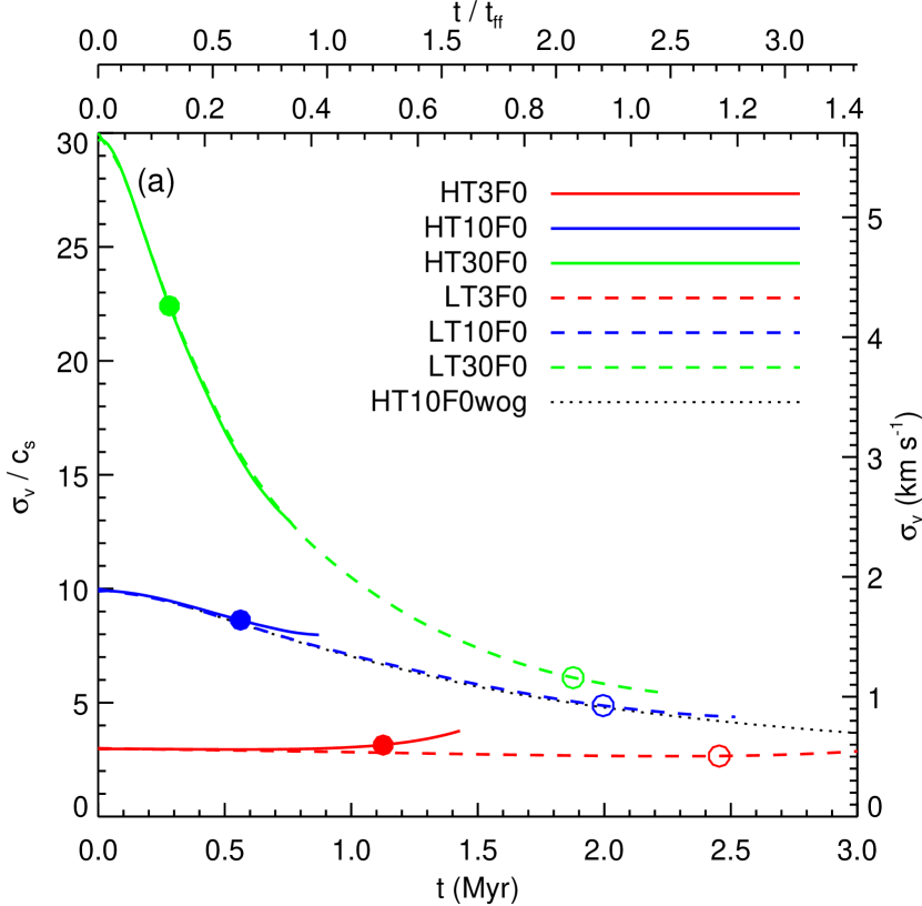
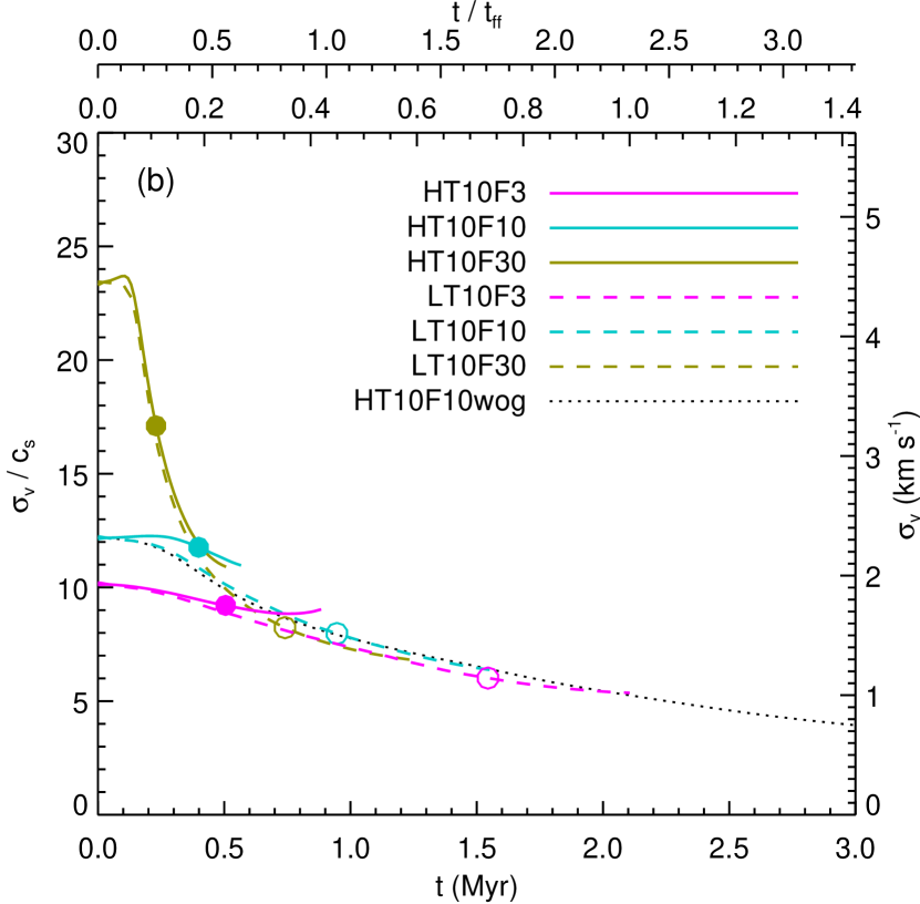
Figure 6.— Velocity dispersions ($\sigma_{v}$) as functions of time for all models (a) without and (b) with the colliding flows. The solid and dashed curves denote $\sigma_{v}$ for the high-density and the low-density models, respectively, from the initial stages to the stage of $M_{\mathrm{\star,max}}=10\,M_{\sun}$. The dotted black curves denote the model without self-gravity. The filled and open circles denote the first sink particle formation for the high-density and low-density models, respectively. The upper two abscissas show the time normalized by the freefall time of the high-density (upper axis) and the low-density models (lower axis).

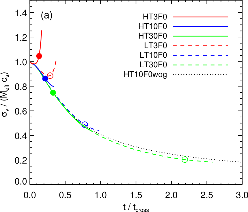
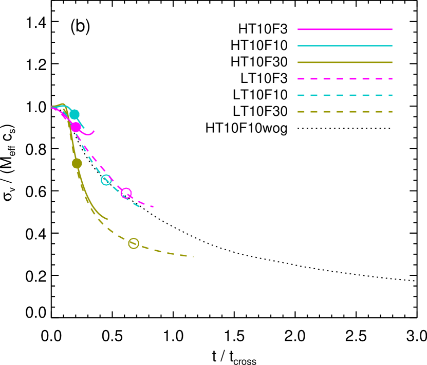
Figure 7.— Same as Figure 6 but velocity dispersion and time are normalized by the effective Mach number ${\cal M}_{\mathrm{eff}}$ and the crossing time $t_{\mathrm{cross}}$, respectively.

For models without colliding flows (Figure 6(a)), models with a common ${\cal M}_{t}$ exhibit similar decay of turbulence irrespective of their initial densities. After the stages of formation of the first sink particle, as denoted by circles, the high-density models tend to have a slightly higher $\sigma_{v}$ than the low-density models because of self-gravity. The models without colliding flows produce the first sink particle roughly around $\sim t_{\mathrm{ff}}$ irrespective of the initial density, whereas the time of formation of the first sink particle tends to be early when assuming strong turbulence.

When the time and velocity dispersion are normalized by the crossing time and the effective Mach number, respectively, the evolutions for the different models converge to that for model MT10F0wog (non-gravitational model), as shown in Figure 7(a). This indicates that the turbulence decays in the crossing time scale, $t_{\mathrm{cross}}$, are in agreement with Mac Low et al. (1998), Mac Low (1999), and Ostriker et al. (2001). The high-density models and the low-density model LT3F0 undergo gravitational collapse to form sink particles before the initially assumed turbulence decays considerably.

Figure 6(b) and Figure 7(b) show velocity dispersions as functions of time for the models with colliding flows. The colliding flows contribute to $\sigma_{v}$, and $\sigma_{v}$ at $t=0$ depends on ${\cal M}_{f}$ when comparing models with the same ${\cal M}_{t}$, as shown in Figure 6(b). All the models tend to converge to the locus of the non-gravitational model as time proceeds (Figure 6(b)). This tendency indicates that colliding flows decay faster than do isotropic turbulent flows. For example, models with ${\cal M}_{f}=30$ show rapid decreases in $\sigma_{v}$, and the timescales of the decreases are smaller than $t_{\mathrm{cross}}$ (Figure 7(b)), where $\sigma_{v}$ decreases by a factor of 50% in a time of $0.3t_{\mathrm{cross}}$. The rapid decreases in $\sigma_{v}$ are responsible for the shock waves formed by the colliding flows. The colliding flow brings forward the first sink particle formation, and the elapsed time until the first sink particle formation is shorter than the freefall time irrespective of the initial densities.

4.6. Compressibility of velocity fields

A velocity field can be separated into solenoidal (transverse) and compressive (longitudinal) components by applying a Helmholtz decomposition. The decomposition of the velocity field has also been used to discuss turbulence (e.g., Kitsionas et al., 2009; Federrath et al., 2010b). We performed the velocity decomposition and estimated $E_{\mathrm{trans}}$ and $E_{\mathrm{long}}$ according to Equations (B8) and (B9), where $E_{\mathrm{trans}}$ and $E_{\mathrm{long}}$ are the powers of the transverse and longitudinal velocity components, respectively (see Appendix B). Figure 8 shows $E_{\mathrm{long}}/E_{\mathrm{tot}}$ as functions of time, where $E_{\mathrm{tot}}=E_{\mathrm{long}}+E_{\mathrm{trans}}$.

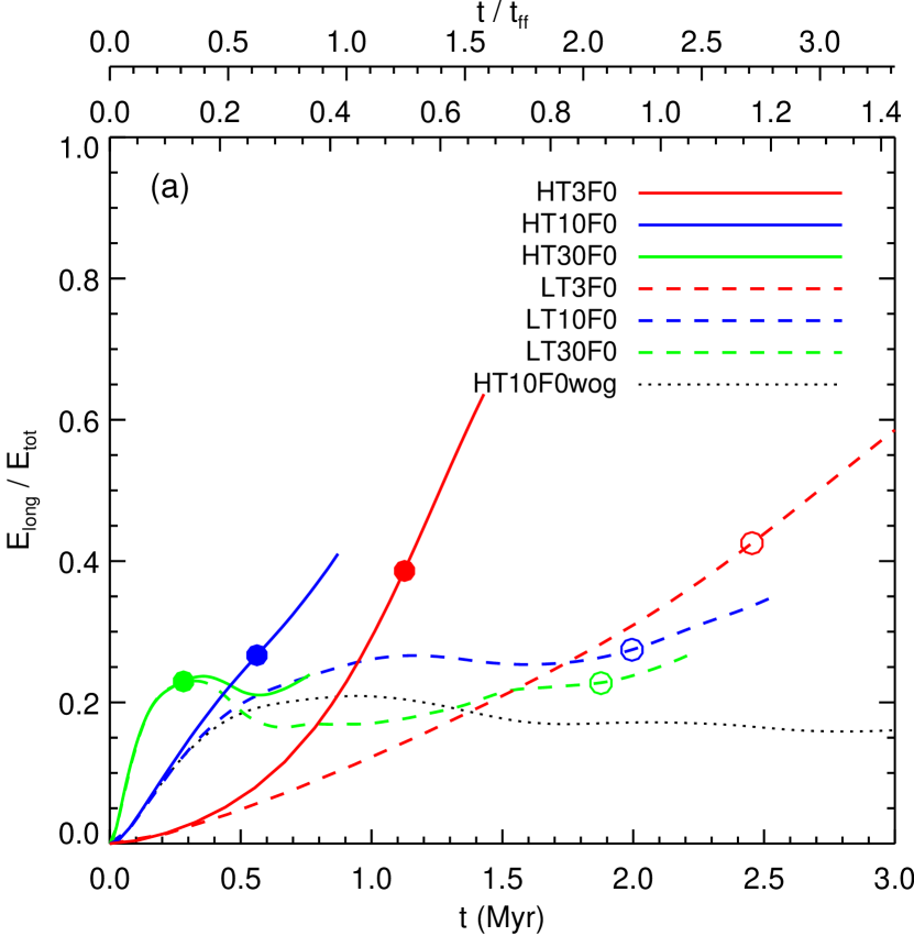
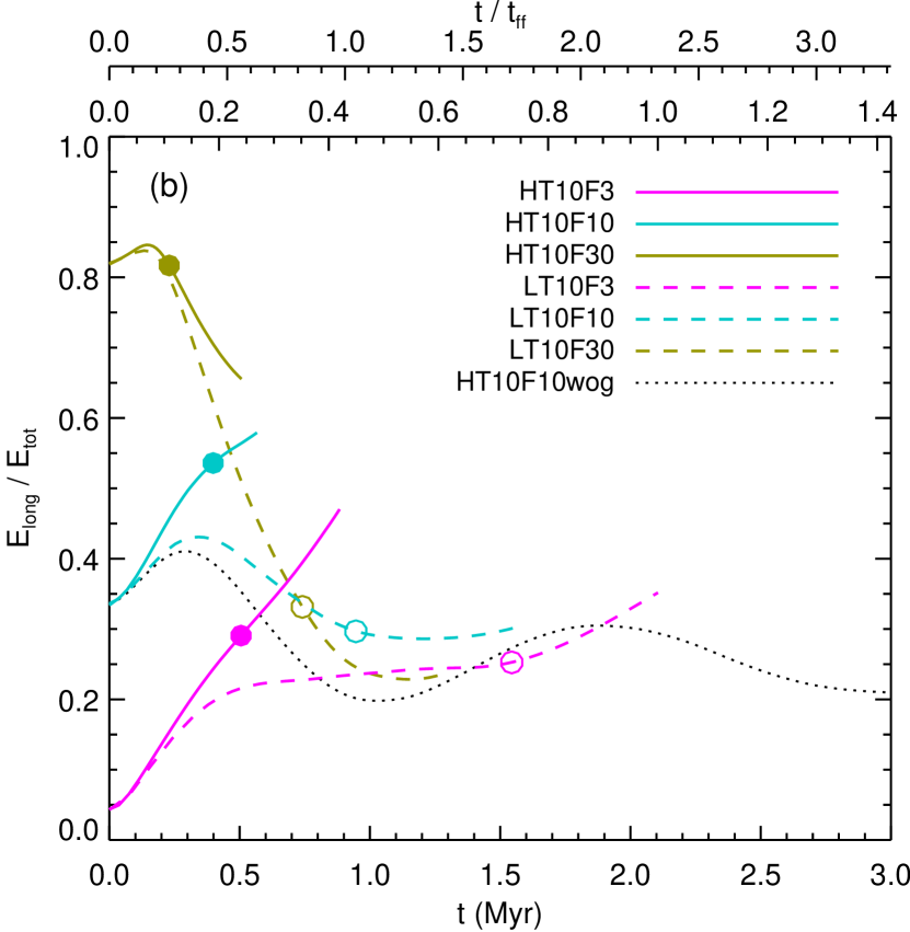
Figure 8.— Ratio of longitudinal power to total power, $E_{\mathrm{long}}/E_{\mathrm{tot}}$, as functions of time for the models (a) without and (b) with the colliding flows. The solid and dashed curves denote the ratios of the powers for the high-density and low-density models, respectively. The dotted black curves denote the model without self-gravity. The filled and open circles denote the first sink particle formation for the high-density and low-density models, respectively. The upper two abscissas show the time normalized by the freefall time of the high-density (upper axis) and low-density models (lower axis).

The models without colliding flow show $E_{\mathrm{long}}/E_{\mathrm{tot}}=0$ at the initial stages ($t=0$), because the initial velocity field is incompressible. As time proceeds, $E_{\mathrm{long}}/E_{\mathrm{tot}}$ increases. This increase indicates that the compressibility of the velocity field increases. In the early stages, models with the same turbulent Mach number and a different initial density exhibit similar increases in $E_{\mathrm{long}}/E_{\mathrm{tot}}$. Models HT10F0 and LT10F0 show increases in $E_{\mathrm{long}}/E_{\mathrm{tot}}$ at a rate similar to the non-gravitational model HT10F0wog. Models with strong turbulence tend to show a rapid increase in $E_{\mathrm{long}}/E_{\mathrm{tot}}$, and the increase rates are in proportion to the crossing time, $t_{\mathrm{cross}}$. These increases indicate that evolution in the early stages is controlled mainly by the turbulence.

In the later stages, the self-gravitational models HT10F0 and LT10F0 exhibit higher ratios of power than does the non-gravitational model HT10F0wog. This indicates that self-gravity increases the compressibility of the velocity field. The high-density models tend to exhibit more rapid increases in $E_{\mathrm{long}}/E_{\mathrm{tot}}$ than do the low-density models, and this result underscores the differences in freefall times between them.

The non-gravitational model HT10F0wog, followed for a long time of $2.5\times 10^{7}\,\mathrm{yr}$, exhibits considerable oscillation of $E_{\mathrm{long}}/E_{\mathrm{tot}}$ in the range of $0.15-0.2$. After the velocity becomes subsonic $\sigma_{v}\lesssim c_{s}$, the oscillation dumps and $E_{\mathrm{long}}/E_{\mathrm{tot}}\simeq 0.15$ is shown.

Models with colliding flows exhibit $E_{\mathrm{long}}/E_{\mathrm{tot}}>0$ at the initial stages because the colliding flows are compressible and contribute to $E_{\mathrm{long}}$. The high-density models tend to have a high ratio of $E_{\mathrm{long}}/E_{\mathrm{tot}}$ than do the low-density models. Moreover, in comparison with the non-gravitational models, the self-gravitational modes have a high ratio. These comparisons also indicate that self-gravity enhances the compressibility of the velocity field.

The non-gravitational model HT10F10wog exhibits an oscillation of $E_{\mathrm{long}}/E_{\mathrm{tot}}$ with decaying amplitude in the range of $0.2-0.4$ when $\sigma_{v}\gtrsim c_{s}$ (the early part of the epoch is shown in Figure 8), and it decreases to $\simeq 0.15$ when $\sigma_{v}\lesssim c_{s}$. The amplitude of the oscillation is larger than that for the non-colliding model HT10F0wog. The oscillation is responsible for the oscillation on $E_{\mathrm{long}}$, while $E_{\mathrm{trans}}$ decreases monotonically.

4.7. Probability distribution functions

It is known that the probability distribution function (PDF) of density in isothermal turbulent gas without self-gravity is well approximated by a lognormal distribution (e.g., Vazquez-Semadeni, 1994). The lognormal distribution is expressed as (Ostriker et al., 2001; Padoan & Nordlund, 2002)

$$p(s)ds=\frac{1}{(2\pi\sigma_{s}^{2})^{1/2}}\exp\left[-\frac{1}{2}\left(\frac{s-\bar{s}}{\sigma_{s}}\right)^{2}\right]ds,$$ (3)

$$s=\ln\left(\frac{\rho}{\rho_{0}}\right),$$ (4)

$$\bar{s}=-\frac{\sigma_{s}^{2}}{2},$$ (5)

where $\bar{s}$ and $\sigma_{s}$ denote the average and the standard deviation of the logarithmic density, $s$, respectively. The standard deviation, $\sigma_{s}$, is found to be a function of the Mach number for the gas, ${\cal M}$, as (Padoan et al., 1997)

$$\sigma_{s}^{2}=\ln\left(1+\gamma^{2}{\cal M}^{2}\right),$$ (6)

where $\gamma\simeq 0.5$ and ${\cal M}=\langle\left(v-\langle v\rangle\right)^{2}\rangle^{1/2}/c_{s}$, and $\langle\cdot\rangle$ denotes a volume-weighted average.

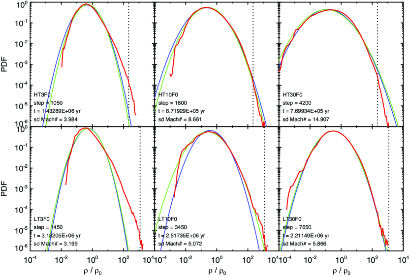
Figure 9.— Volume-weighted probability distribution functions (PDFs) for models without colliding flow. The upper and lower figures show PDFs for the high-density and low-density models, respectively. The left, middle, and right figures show PDFs for models with ${\cal M}_{t}=3,10,$ and 30, respectively. The red curves denote the PDFs derived from the density distributions at the stages of $M_{\mathrm{\star,max}}=10\,M_{\sun}$. The green and blue curves show the lognormal functions with the standard deviations derived from the density distributions and Equation (6), respectively. The vertical dotted lines show the threshold densities for the sink particle, $\rho_{\mathrm{sink}}$.

At the initial stage, the PDFs are expressed by a delta function because the initial density is constant. As time proceeds, the profiles of the PDFs are broadened, and they are well expressed by the lognormal distributions for all models without colliding flow in the early phase, typically before sink particles form. Figure 9 shows the volume-weighted PDFs for models without colliding flow at the stages of $M_{\mathrm{\star,max}}=10\,M_{\sun}$. For models with ${\cal M}_{t}=3$, the PDFs have power-law tails in the high densities and so deviate from the lognormal functions. This indicates that the cloud structure in high density is affected by self-gravity. A deviation of PDFs from the lognormal distribution was also reported by Klessen (2000), Federrath et al. (2008), and Federrath & Klessen (2013) for self-gravitational isothermal turbulence. During the evolution, the profiles of the low-density tails oscillate around the lognormal distributions. The PDFs of the snapshots shown in Figure 9 therefore deviate from the lognormal distribution at low densities.

In Figure 9, two fitting curves are plotted for each model based on the lognormal functions. The standard deviation of the logarithmic density is derived from the density distribution (green curve), and the standard deviation is derived by using Equation (6) (blue curve). In the case of non-gravitational driven turbulence, Konstandin et al. (2012) reported $\gamma=1/3$ for solenoidal forcing and $\gamma=1$ for compressive forcing (see Price et al., 2011). We adopt $\gamma=1/2$ here because it provides a better fit to the data than do the other values. These two lognormal fitting curves roughly coincide and indicate that Equation (6) is satisfied well in the stages examined here, even in the case of self-gravitating gas.

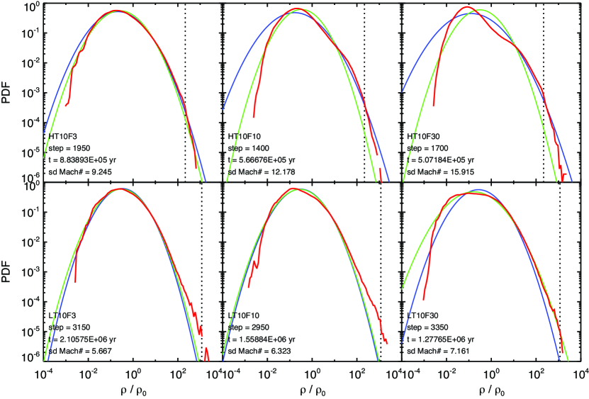
Figure 10.— Volume-weighted probability distribution functions (PDFs) for models with a common initial turbulent strength ${\cal M}_{t}=10$ and different strengths of colliding flow ${\cal M}_{t}$. The upper and lower figures show PDFs for the high-density and low-density models, respectively. The left, middle, and right figures show PDFs for models with ${\cal M}_{f}=3,10,$ and 30, respectively. The red curves denote the PDFs derived from the density distributions at the stages of $M_{\mathrm{\star,max}}=10\,M_{\sun}$. The green and blue curves show the lognormal functions with the standard deviations derived from the density distributions and Equation (6), respectively. The vertical dotted lines show the threshold density for the sink particle, $\rho_{\mathrm{sink}}$.

Figure 10 shows the volume-weighted PDFs for models with colliding flow. In the cases with strong colliding flow, especially in the high-density models, the PDFs deviate considerably from the lognormal distributions around the peaks. This deviation is attributed to the sheet structures of the clouds caused by the colliding flow, as shown in Figures 4(e) and 4(f). Moreover, the two fitting curves, which show significantly different distributions, indicate that Equation 6 is no longer satisfied in the cases with strong colliding flow.

PDFs for the column density are shown because they are often examined in observational studies, (e.g., Lombardi et al., 2011). Ostriker et al. (2001) showed that the PDF for the column density can also be fitted by lognormal functions.

Figure 11(a) shows the PDFs for the column density for model LT10F0. The density PDF for Model LT10F0 has a little excess from the lognormal function in the high densities (the bottom panel in the middle of Figure 9). The profiles of the column density PDFs are bumpy compared to the density PDFs because the sampling numbers for the column density are less than those for the density. For the first three stages shown in Figure 11(a), each PDF can be fitted well by a lognormal function (dotted curves). To examine the long-time evolution of the PDF for this model, we follow the cloud evolution until the stage of $M_{\mathrm{\star,max}}=50\,M_{\sun}$ ($t=3.4\,\mathrm{Myr}$). The PDF at this stage has a wing at high column density, which can be fitted by the power law of $\mathrm{PDF}\propto\Sigma^{-2}$. The estimated power indexes depend on the models; the power index is approximated as $-3$ for models HT3F0 and HT10F0, and seems to change from $-2$ to $-3$ as the column density increases for model LT3F0. Such a power-law wing in PDFs has often been observed in several star-forming regions (i.e., Kainulainen et al., 2009), as will be discussed in Section 5.1.1.

Figure 11.— Evolution of PDFs of the column densities for (a) model LT10F0 and (b) model HT10F10. The column densities are estimated along (a) the $x$-direction and (b) the $z$-direction. The solid lines show the PDFs at the four stages, from bottom to top: the relatively early stage, the stage of the first sink particle formation, the stage of $M_{\mathrm{\star,max}}=10\,M_{\sun}$, and the stage of $M_{\mathrm{\star,max}}=50\,M_{\sun}$. The times for the stages are shown at the left of the PDF curves. In order to plot all of the PDFs, the plots are offset from each other by a factor of 10 in the vertical direction. The column densities on the abscissa are normalized by the initial values. The dotted curves are the fitting curves of lognormal functions, which are determined by the mean and the standard deviation of the column densities. In panel (a), the broken line shows the relationship of $\mathrm{PDF}\propto\Sigma^{-2}$.

Figure 11(b) shows the column density PDFs for the colliding model HT10F10. The line of sight is the $z$-direction, which is perpendicular to the colliding flow. Along this line of sight, the sheet cloud appears in the edge-on view. The PDFs highly deviate from lognormal functions and exhibit two peaks, which are responsible for the sheet cloud with a high column density and the colliding flow with a low column density. We confirmed that, when the line of sight is taken to be the face-on direction, the PDFs can be fitted by a lognormal function. In summary, the features of the PDFs for the column density depend on the line of sight, and they can highly deviate from a lognormal function when the cloud is disturbed by a large-scale flow.

4.8. Mass distribution for sink particles

Figure 12 shows the mass distribution for sink particles in the histograms for all models. The high-density models exhibit clear features in the histograms, whereas the low-density models do not because of the small number of sink particles produced. For the high-density models, the mass distribution has a peak around $\sim 1M_{\sun}$ and has tails in both the high masses and low masses. For all the high-density models except model HT10F30, the tails can be roughly fitted by the relationship $N_{\mathrm{star}}(M_{\mathrm{star}})\propto M_{\mathrm{star}}^{-1.35}$, which is a classical initial mass function (IMF) of Salpeter (1955). Similar tails at high masses were reported for a cloud with a different mass of $500M_{\sun}$ by Bate (2009) and Bate (2012). Model HT10F30 shows considerably steeper tails than does the fitting line at high mass. This is because this model produces $3.6-6.5$ times more sink particles than do the other models (models HT10F3 and HT10F10) and the masses of the peaks and the maximum masses are roughly common among the models.

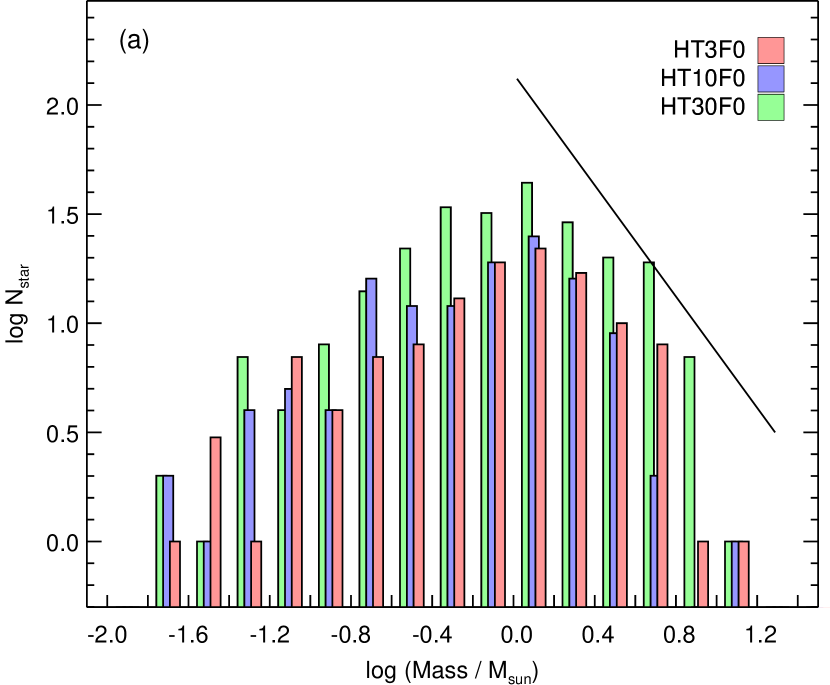
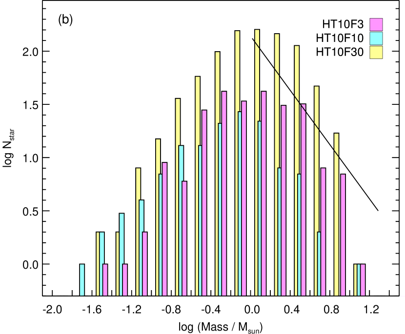
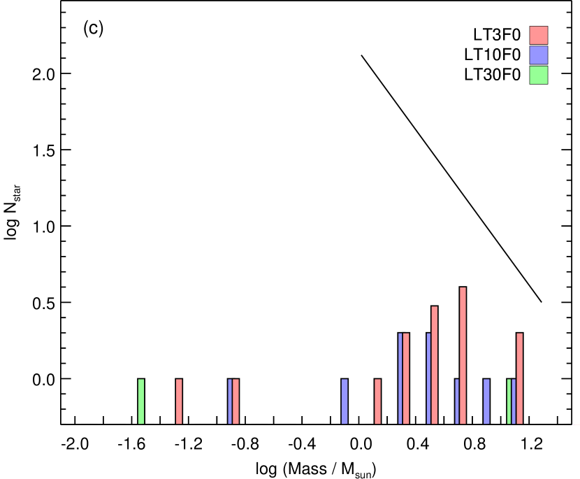
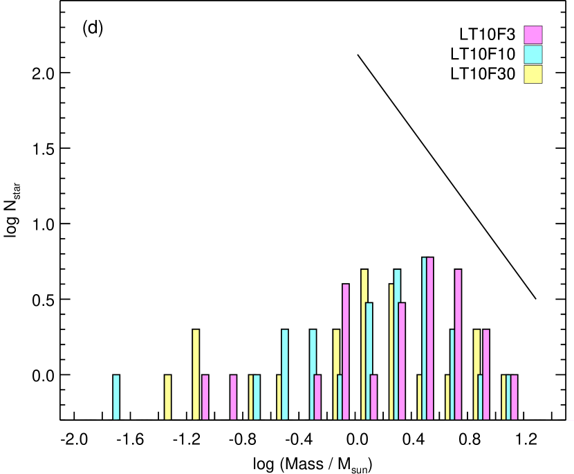
Figure 12.— Histograms of the masses of sink particles for (a, b) the high-density models and (c, d) the low-density models at the stages of $M_{\mathrm{\star,max}}=10\,M_{\sun}$. The relationship of $N_{\mathrm{star}}(M_{\mathrm{star}})\propto M_{\mathrm{star}}^{-1.35}$ (Salpeter, 1955) is plotted by the solid line in each panel for comparison. The bin size of the mass is set at $\log 0.2$.

The histograms presented here have a turnover near $\sim 1M_{\sun}$, whereas the IMFs derived from observations in several star-forming regions tend to have a turnover near $\sim 0.07-0.5M_{\sun}$ (e.g., Kroupa et al., 2013). A possible interpretation for the discrepancy is that the our simulations do not spatially resolve the formation of very low mass stars whose masses are $\lesssim 0.1\,M_{\sun}$, e.g., brown dwarfs. As shown in Figure 13, some sink particles have $\sim 0.1\,M_{\sun}$ when they are produced. If a finer resolution is adopted, the initial masses of the sink particles could be lower. This could shift the turnover to lower mass.

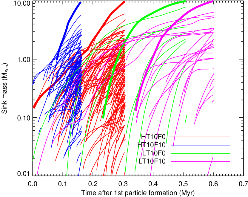
Figure 13.— Masses of sink particles as functions of time after the first sink particle formation for models HT10F0, HT10F10, LT10F0, and LT10F10. The thick lines show particles reaching $10\,M_{\sun}$.

Figure 13 shows the evolution of sink particle mass for the four representative models. As also shown in Table 1, the number of sink particles is larger in the high-density models than in the low-density models. The high-density models and the models with colliding flows take a shorter time for the sink particles to reach $10\,M_{\sun}$ after the initial sink particle formation than do the other models. However, the typical accretion rates (slopes of the lines) do not exhibit a significant difference between models. Among all sink particles, those reaching $10\,M_{\sun}$, as indicated by the thick lines, show slightly higher accretion rates (steeper slopes) for the high-density and/or colliding models.

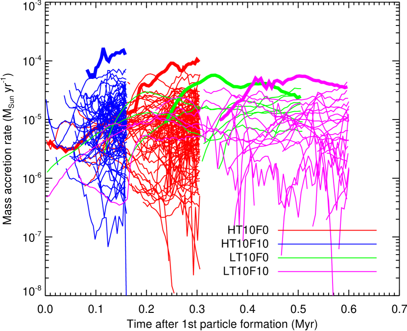
Figure 14.— Mass accretion rates of sink particles as functions of time after the first sink particle formation for models HT10F0, HT10F10, LT10F0, and LT10F10. The thick lines show particles reaching $10\,M_{\sun}$.

Figure 14 shows the accretion rates for the sink particles explicitly. The accretion rates are spread over a wide range of $10^{-7}\,M_{\sun}\mathrm{yr}^{-1}\lesssim\dot{M}\lesssim 10^{-4}\,M_{\sun}\mathrm{yr}^{-1}$, which is a common range for the models. The accretion rate for each particle oscillates within this range. This range includes the typical accretion rate for gas of 10 K, i.e., $c_{s}^{3}/G=2\times 10^{-6}\,M_{\sun}\mathrm{yr}^{-1}$, while the majority of sink particles exceed this value. The most massive particle tends to have the highest accretion rate in each model (see thick lines in Figure 13 and Figure 14). There is also a tendency that a model producing more stars has higher maximum mass of stars when observed at a given epoch. For example, among the four models shown in Figure 13, model HT10F10 has the highest maximum stellar mass, and this model produces the most number of stars at 0.1 Myr after the first sink particle formation. This indicates that the maximum mass of stars correlates with the number of stars formed there. A similar implication is proposed by the observational research of Dobashi et al. (2001), in which the maximum stellar luminosity of protostars correlates with the mass of the parent clouds. Moreover, some other observations have shown that the number of protostars also correlates with the mass of the parent cloud (Dobashi et al., 1996; Yonekura et al., 1997; Kawamura et al., 1998). When we simply assume that the stellar luminosity correlates with the stellar mass, these observations also show that the maximum stellar masss correlates with the number of stars in agreement with our simulations.

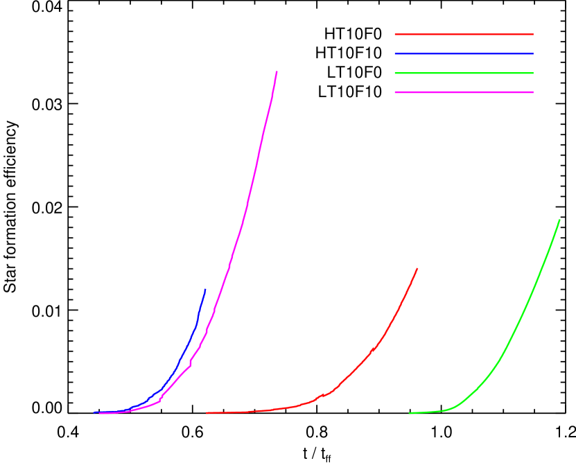
Figure 15.— Star formation efficiency as functions of time for models HT10F0, HT10F10, LT10F0, and LT10F10.

Figure 15 shows the star formation efficiency as a function of the freefall time for each model. The star formation efficiency is defined as the ratio of the mass of all sink particles to the total mass of all particles and gas. Star formation in models with colliding flows (models HT10F10 and LT10F10) begins in earlier stages than for models without colliding flow (models HT10F0 and LT10F0). In comparing models with the same colliding flow, the high-density models tend to begin star formation earlier than do the low-density models. After star formation begins, the star formation efficiencies increase with a similar trend in all models. This similar trend indicates that the high-density models have higher accretion rates in total than do the low-density models because the clouds of the high-density models are more massive than those of the low-density models. These high accretion rates are mainly due to the large number of sink particles formed in the high-density models.

4.9. Velocity distribution for sink particles

Sink particles are produced with initial velocities so that the linear momenta of the material gas and the formed sink particles are conserved. Sink particles change their velocities via gas accretion onto the sink particles and gravitational interaction with the gas and other particles. Figure 16 shows the velocity distributions for sink particles in bar charts for the four representative models HT30F0, HT10F30, HT10F10, and LT10F0 at the stage of $M_{\mathrm{\star,max}}=10\,M_{\sun}$. The high-density models have many sink particles, and each model exhibits a profile of velocity distribution with a peak and tails at both low and high velocities. In contrast, the low-density models do not have sufficient numbers of sink particles to show such a clear profile.

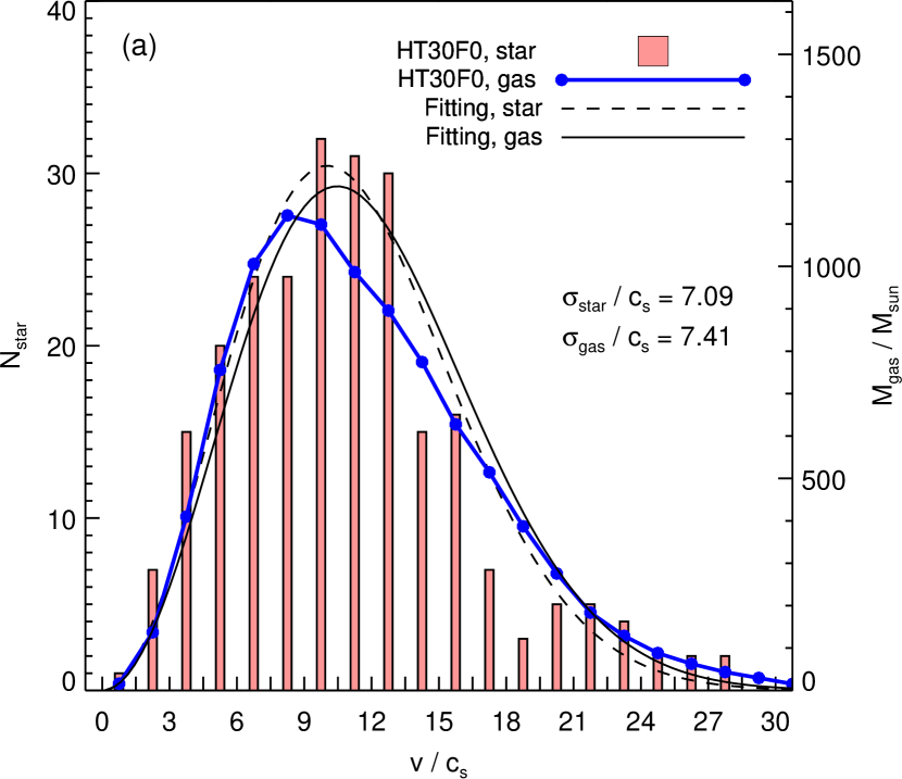
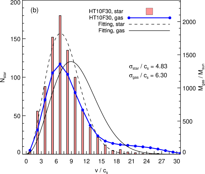
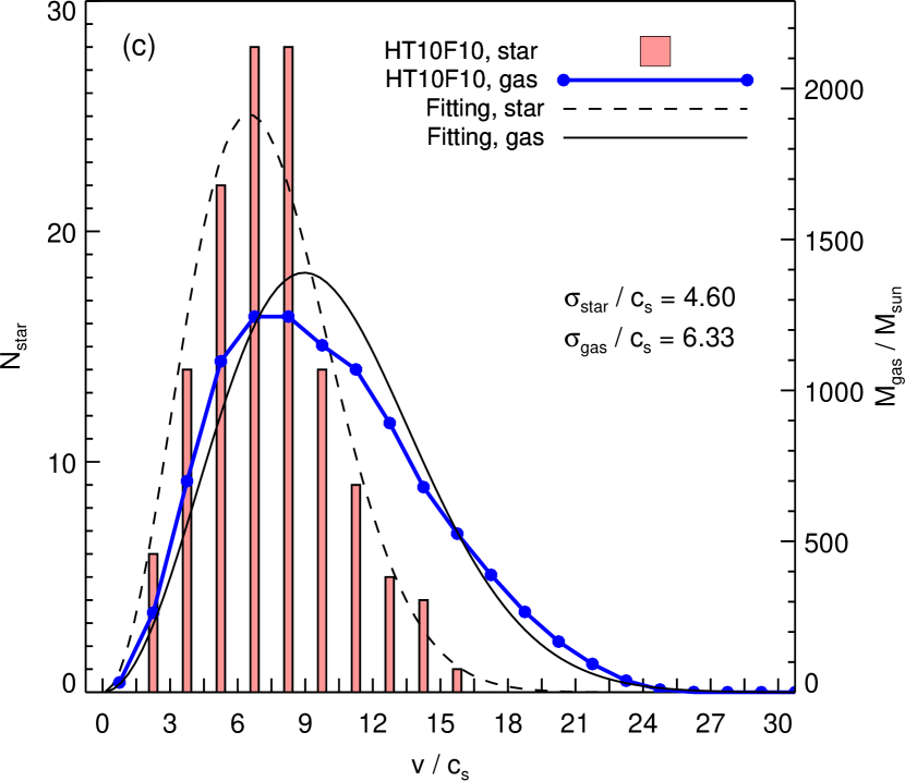
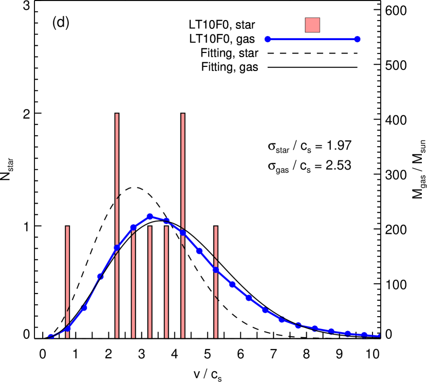
Figure 16.— Histograms of sink particles (bar charts) and gas (blue lines with filled circles) as functions of velocity $v/c_{s}^{2}$ for models (a) HT30F0, (b) HT10F30, (c) HT10F10, and (d) LT10F0 at the stage of $M_{\mathrm{\star,max}}=10\,M_{\sun}$. The dashed and solid lines are fitting curves derived from the functions of $p(|\mbox{\boldmath$v$}|;\sigma_{\mathrm{star}})$ and $p(|\mbox{\boldmath$v$}|;\sigma_{\mathrm{gas}})$ (see eq (7)).

The velocity distributions for gas are plotted for comparison in Figure 16. For the high-density models HT30F0 and HT10F30, the velocity distributions for sink particles are similar to those for gas; the peak positions and widths of the profiles coincide between the sink particles and the gas. For model HT10F30, the velocity distribution for gas has a wing at high velocities because of the accretion flow onto the sheet cloud. The accretion flow does not considerably affect the velocities of the sink particles because the accretion flow has low density and the sink particles exist around the high-density sheet clouds. Model HT10F10 also has an accretion flow onto the sheet, but the flow is denser and slower than that for model HT10F30 (see Figure 4 for comparison of the densities of accretion flows between these models). The profile of the velocity distribution for gas therefore appears to shift to the high velocities with respect to the velocity distribution for the sink particles.

For all low-density models, the velocity distributions for sink particles roughly agree with those for gas, even though the number of sink particles is small. Note that sink particle formation occurs after the sheet caused by the colliding flow disappears for the low-density models. Even for the colliding models, the velocities of sink particles follow the velocity distribution for gas.

The fitting curves for both sink particles and gas are also plotted in Figure 16 under the assumption that the velocities of sink particles and gas follow a Gaussian distribution. When each velocity component, $(v_{x},v_{y},v_{z})$, follows a Gaussian distribution with a velocity dispersion, $\sigma$, the distribution for the absolute value of the velocity $|\mbox{\boldmath$v$}|$ is given by

$$p(|\mbox{\boldmath$v$}|;\sigma)=\frac{2|\mbox{\boldmath$v$}|^{2}}{(2\pi)^{1/2}\sigma^{3}}\exp\left(-\frac{|\mbox{\boldmath$v$}|^{2}}{2\sigma^{2}}\right).$$ (7)

The velocity dispersion for the sink particles is evaluated by

$$\sigma_{\mathrm{star}}=\left(\frac{1}{3N_{\star}}\sum_{i=1}^{N_{\star}}|\mbox{\boldmath$v$}_{i}|^{2}\right)^{1/2},$$ (8)

and that for gas is evaluated by using a mass-weighted integral,

$$\sigma_{\mathrm{gas}}=\left(\frac{\displaystyle\int\rho(\mbox{\boldmath$r$})|\mbox{\boldmath$v$}(\mbox{\boldmath$r$})|^{2}dV}{\displaystyle 3\int\rho(\mbox{\boldmath$r$})dV}\right)^{1/2}.$$ (9)

The numerical factor of 3 in Equations (8) and (9) comes from the number of spatial dimensions.

The fitting curves indicate that the velocities of sink particles and gas are well described by a Gaussian distribution for model HT30F0. The velocity dispersion for sink particles is roughly the same as that for gas ($\sigma_{\mathrm{star}}\simeq\sigma_{\mathrm{gas}}$). Such a tendency is confirmed in all the high-density models without colliding flow. In the high-density models with colliding flow, gas has a significantly larger velocity dispersion than that for sink particles ($\sigma_{\mathrm{gas}}\gtrsim\sigma_{\mathrm{star}}$) because of the high-velocity wing due to the colliding flow. Due to the large velocity dispersion, the fitting curve for gas shifts to high velocities with respect to sink particles. In these models we also confirmed that, for sink particles, the velocity dispersion for $v_{x}$ tends to be smaller than those for $v_{y}$ and $v_{z}$. The dispersion difference indicates that the gravity of the sheet decelerates the motion of the sink particles along the $x$-direction, which is the direction normal to the sheet.

Sink particles and gas change their velocity distributions as time proceeds. For model HT30F0, a considerable decrease in the velocity dispersion for gas is seen in Figure 6, even after formation of the first sink particle. In this model, the velocity dispersion for gas decreases: $\sigma_{\mathrm{gas}}/c_{s}=10.76$ and $7.41$ at the stages of $M_{\mathrm{\star,max}}=1\,M_{\sun}$ and $10\,M_{\sun}$, respectively. The velocity dispersion for sink particles also decreases: $\sigma_{\mathrm{star}}/c_{s}=9.09$ and $7.09$ at the stages of $M_{\mathrm{\star,max}}=1\,M_{\sun}$ and $10\,M_{\sun}$, respectively. This indicates that stars with a velocity dispersion similar to that for gas are produced continuously. On the other hand, for model HT10F0, the velocity dispersion for gas decreases slightly, as seen in Figure 6, and both $\sigma_{\mathrm{star}}$ and $\sigma_{\mathrm{gas}}$ are roughly constant.

4.10. Channel maps

Reconstruction of channel maps by using the data of the numerical simulations is useful for comparison of observations and numerical simulations, as demonstrated by Dobashi et al. (2014). The channel maps here are reconstructed for four models: HT10F0, HT10F10, LT10F0, and LT10F10. In reconstructing a channel map, gas is assumed to be optical thin and both the non-thermal and thermal velocity components are considered; each numerical cell has a velocity along the line of sight, $v_{\mathrm{los}}$, with a Gaussian profile, which is broadened by the sound speed, and the central velocity of the Gaussian is equal to the bulk velocity. The $x$-direction is adopted as the line of sight, which is parallel to the direction of the colliding flow.

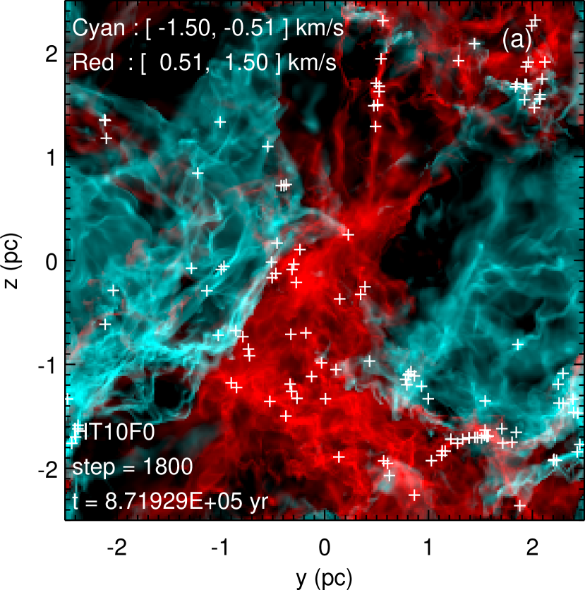
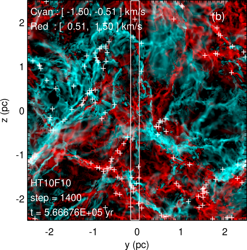
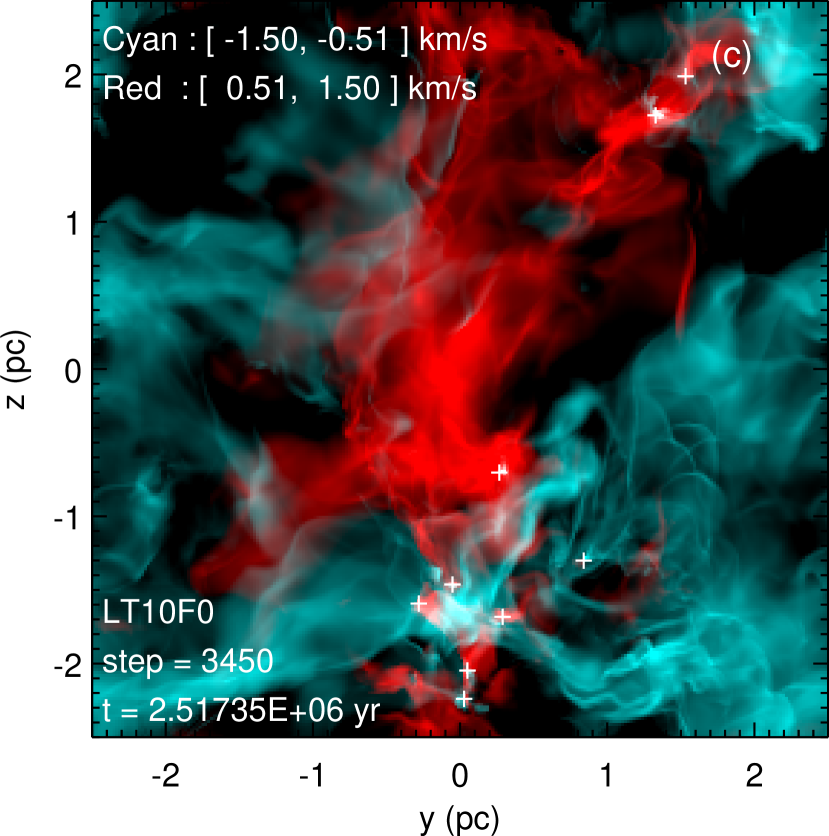
Figure 17.— Composite maps of different velocity channels for models (a) HT10F0, (b) HT10F10, (c) LT10F0, and (d) LT10F10 at the stages of $M_{\mathrm{\star,max}}=10\,M_{\sun}$. Two velocity channels of $-1.50\,\mathrm{km\,s^{-1}}<v_{\mathrm{los}}<-0.51\,\mathrm{km\,s^{-1}}$ (cyan) and $0.51\,\mathrm{km\,s^{-1}}<v_{\mathrm{los}}<1.50\,\mathrm{km\,s^{-1}}$ (red) are overlaid. Note that red and cyan are complementary colors. The regions where the gas exists in both channels are shown in white, those having gas in either channel are shown in red or cyan, and those without gas in both channels are shown in black. The plus symbols ($+$) denote the positions of the sink particles. The slit in panel (b) is for the position-velocity diagram shown in Figure 18.

Figure 17 shows composite maps for the two velocity channels. In each composite map, two representative velocity channels of $-1.50~{}\mathrm{km~{}s}^{-1}\leq v_{\mathrm{lols}}\leq-0.51~{}\mathrm{km~{}s}^{-1}$ and $0.51~{}\mathrm{km~{}s}^{-1}\leq v_{\mathrm{lols}}\leq 1.50~{}\mathrm{km~{}s}^{-1}$ are shown in cyan and red colors, respectively. Components existing in both velocity channels are expressed in white because cyan and red are complementary colors.

The most prominent features are shown in model HT10F10 (Figure 17(b)), where red and cyan filaments are tangled up with each other on a 0.1 pc scale. Moreover, the red and cyan filaments show an anti-correlated distribution because of the collision of filaments, as shown by Dobashi et al. (2014). Similar anti-correlation between the different velocity components was also reported by Shimoikura et al. (2013). A considerable number of sink particles exist near the region of collisional interaction, and this indicates that the collision of filaments induces star formation. Stars are also formed along the dense filaments, e.g., the red filament running from $(y,z)=(-0.7,-1.3)~{}\mathrm{pc}$ to $(-0.2,-0.6)~{}\mathrm{pc}$.

In contrast, models HT10F0, LT10F0, and LT10F10 exhibit coarser patterns of red and cyan colors on a parsec scale (Figures 17(a), (c), and (d)). These patterns indicate that velocity shear on the cloud scale exists. This is attributed to turbulence, which has a larger kinetic energy in a longer wavelength mode. Therefore, the cloud-scale gas motion should dominate over short wavelength modes when considering turbulence with the power spectrum examined here. We confirmed that similar anti-correlations on the cloud scale are also shown irrespective of the choice of line of sight for the models without colliding flows.

The low-density colliding model LT10F10 has a sheet cloud caused by the colliding flow before sink particles form. The sheet cloud disappears at the stage shown in Figure 17(d). When the sheet cloud exists, the channel map shows the anti-correlation pattern on a sub-parsec scale, as also seen for model LT10F10. However, the contrast for the anti-correlation pattern is much weaker than that for the high-density model HT10F10 because the filaments in the low-density model have a low density contrast.

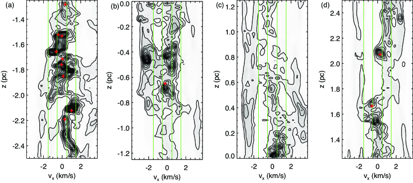
Figure 18.— Position-velocity diagram for model HT10F10 at the stage of $M_{\mathrm{\star,max}}=10\,M_{\sun}$. The long slit region indicated in Figure 17(b) is shown in the four panels separately according to the $z$-coordinates. The contours and gray scales show the gas density. The lowest contours and contour intervals are $2.5\times 10^{38}\,\mathrm{cm}^{-1}(\mathrm{km\,s})^{-1}$. The red plus symbols ($+$) denote the locations of the sink particles in the position-velocity plane. The vertical green lines show the boundaries of the two velocity ranges shown in Figure 17.

Figure 18 shows a position-velocity (PV) diagram for examining the slit region in Figure 17(b). Every sink particle is associated with a dense gas component in the PV diagram. Figure 18(a) shows the PV diagram for the region of $-2.5\,\mathrm{pc}\leq z\leq-1.25\,\mathrm{pc}$, where the interaction between clouds with different velocities induces the star formation shown in Figure 17(b). The PV diagram clearly shows that dense gas components pass through each other with supersonic velocities in the $x$-direction (line of sight).

In Figure 18(b), two dense components with different velocities exist in $-0.5\,\mathrm{pc}\lesssim z\lesssim-0.4\,\mathrm{pc}$ without an associated sink particle. This figure shows that these components have not yet collided. The components are shown in white in the composite map of Figure 17(b). Indeed, we confirmed that these components collide 0.2 Myr later, and star formation is induced.

The regions shown in Figure 18(c) and 18(d) have only two sink particles, and active star formation is not induced there. In this region, anti-correlation between the dense cyan and the thin red components is observed at $z\simeq 1.7\,\mathrm{pc}$ and a sink particle is associated (Figure 17(b)). The PV diagram suggests that the sink particle is associated with the cyan component, and it interacts with the ambient gas with low density (Figure 18(d)).

5. Discussion

5.1. Comparison with observations

5.1.1 Probability distribution functions

All the models without the colliding flow (${\cal M}_{f}=0$) exhibit PDFs that can be fitted by lognormal functions. The models with weak turbulence tend to show a power-law tail at high density (Figures 9 and 11).

Kainulainen et al. (2009) showed that PDFs for most molecular clouds based on the 2MASS data are well-fitted by lognormal functions at low column densities, and active star-forming clouds always have prominent non-lognormal wings or power-law wings. Although they did not mention power indexes of the power-law wings explicitly, the power indexes appear in ranges from $-3$ to $-2$, according to their figures. Recently, Lombardi et al. (2014) combined Plank dust-emission maps, Herschel dust-emission maps, and 2MASS NIR dust-extinction maps for the Orion complex. They showed that the PDFs for Orion A and B can be fitted by a simple power law with indexes of $-3$. The power-law wings obtained by observations are in agreement with those for our numerical simulations, which have power indexes ranging from $-3$ to $-2$ (see Section 4.7).

Kainulainen et al. (2009) reported that half of the clouds examined in their paper showed non-lognormal features of PDFs at low column densities. This feature is reproduced in our simulations. According to the simulations examined here, the PDF at low density oscillates considerably around a lognormal function, and the PDF obtained from a snapshot of a simulation should deviate from a lognormal function.

PDFs can be affected by the environment of the clouds, as demonstrated by the models with colliding flows (${\cal M}_{f}\neq 0$). According to Lombardi et al. (2006), the PDF for the Pipe molecular clouds is poorly fitted by a single lognormal function. The PDF has a dip near its peak that resembles the PDF for model HT10F10 shown in Figure 11(b). This suggests that the PDF for the Pipe nebula is influenced by external factors. This cloud can be affected by the wind from $\tau$ Sco, a B0 star, as suggested by Onishi et al. (1999). In similar cases, PDFs deviating from a lognormal function were reported by Froebrich & Rowles (2010) in Cepheus, Monoceros, and Ophiuchus clouds.

5.1.2 Velocity distributions

In our simulations, the velocity distributions for the sink particles are similar to those for gas. Our results agree with the kinematic studies of the T-Tarui stars, which were investigated based on their radial velocities and proper motions in several star-forming regions (e.g., Herbig, 1977; Jones & Herbig, 1979; Hartmann et al., 1986; Dubath et al., 1996; Makarov, 2007). These studies reported that the mean stellar velocities are roughly the same as the local gas velocities. In addition, the one-dimensional velocity dispersions obtained by these studies ($\simeq 1-2\,\mathrm{km\,s}^{-1}$) are consistent with the line widths of the molecular lines. Similar results were obtained for protostars by Covey et al. (2006). Fűrész et al. (2008) found that the radial velocities of stars appear to correlate strongly with the radial velocity of the molecular gas cloud for the Orion Nebula Cluster (ONC). Tobin et al. (2009) also investigated the kinematics of ONC and showed that the stellar velocities tend to follow the local gas velocities. These studies as well as our results support the paradigm of dynamical star formation proposed by Hartmann et al. (2001), where rapid star formation is induced by turbulence and/or external flows, and the formed stars are scattered at the local gas velocity as shown in our simulations. In this paradigm, star formation should be terminated by rapid dispersal of gas due to stellar feedback, which is not taken into account in our simulations. Therefore in our simulations, the stars continue to accrete gas, and star formation efficiency becomes high at the late stages of the cloud evolution.

5.2. Comparison with other simulations

As shown in the analysis of the velocity power in Section 4.6, non-gravitational non-colliding model HT10F0wog keeps $E_{\mathrm{long}}/E_{\mathrm{tot}}=0.15-0.2$. This ratio agrees with that obtained by Federrath et al. (2010b), who found that non-gravitational isothermal driven turbulence with ${\cal M}_{t}\simeq 5.5$ has a ratio of $E_{\mathrm{long}}/E_{\mathrm{tot}}\simeq 0.2$ when the driving force is 1/3 or less of the longitudinal mode, i.e., $F_{\mathrm{long}}/F_{\mathrm{tot}}\leq 1/3$ (see their Figure 8). The ratio of $E_{\mathrm{long}}/E_{\mathrm{tot}}\simeq 1/3$ is expected from geometrical considerations (e.g., Nordlund & Padoan, 2003). Federrath et al. (2010b) showed that the velocity Fourier spectra shows $E_{\mathrm{long}}(k)/E_{\mathrm{tot}}(k)\simeq 1/3$ in the inertia range of $k$ for the solenoidal driving force. For the decaying turbulence presented here, the ratio of $E_{\mathrm{long}}(k)/E_{\mathrm{tot}}(k)$ in the inertia range tends to decrease from 0.4 to 0.25 as time proceeds, and the ratio agrees with the case of the turbulence driven by solenoidal force.

In the case with colliding flow, model HT10F10wog shows a higher value of $E_{\mathrm{long}}/E_{\mathrm{tot}}$ in the early stage. This result suggests that the colliding flow provides more compressibility. The compressible flow shows a rapid decay, and $E_{\mathrm{long}}/E_{\mathrm{tot}}=0.2-0.25$ in a long period of $(2-5)t_{\mathrm{cross}}$, which are slightly higher values than those in the non-colliding model. Compared between models HT10F0wog and HT10F10wog, $E_{\mathrm{trans}}$ shows almost the same values during the decay of turbulence, while $E_{\mathrm{long}}$ exhibits slightly higher values in model HT10F10wog than in model HT10F0wog after the rapid decay of $E_{\mathrm{long}}$ in the early stages of model HT10F10wog. The slightly higher value of $E_{\mathrm{long}}/E_{\mathrm{tot}}$ in the colliding model is due to the slightly higher value of $E_{\mathrm{long}}$. Federrath et al. (2010b) showed that non-gravitational turbulence shows $E_{\mathrm{long}}/E_{\mathrm{tot}}=0.6$ when the driving force is purely compressive. This ratio is higher than the colliding model presented here. This is because compressibility is continuously supplied by the driving force in the case of Federrath et al. (2010b), while it is provided by the colliding flow only in the initial stage in our model.

In our simulations, the gravitational collapse leading to star formation occurs locally compared with the cloud scale, and the density structure on the cloud scale is mainly a result of the interaction of turbulent flows. However, self-gravity enhances the compressibility of the velocity field in the whole cloud. For example, models HT3F0 and LT3F0 exhibit $E_{\mathrm{long}}/E_{\mathrm{tot}}\simeq 0.6$ at the last stages. Such a high compressibility of the velocity field requires an extreme driving force of $F_{\mathrm{long}}/F_{\mathrm{tot}}\gtrsim 0.9$ in the case of non-gravitational turbulence (Federrath et al., 2010b).

Hansen et al. (2011) examined the decay of anisotropic turbulence and showed that the decay rate of the turbulence depends on the crossing time of the isotropic component only, and the decay rate is much lower for anisotropic turbulence than for isotropic turbulence. For their highly anisotropic turbulence, $\langle|\nabla\times\mbox{\boldmath$v$}|^{2}\rangle$ is much larger than $\langle|\nabla\cdot\mbox{\boldmath$v$}|^{2}\rangle$, and so it seems that the solenoidal flow dominates over the compressive flow. In our case, models with colliding flows can be considered as anisotropic turbulent models, in which the colliding flow corresponds to a Fourier component of $k_{x}=1$ in the compressive mode. In contrast to the anisotropic models of Hansen et al. (2011), the velocity dispersion due to the colliding flow decays faster than that for the isotropic turbulence (see Figure 6(b)). The anisotropic turbulence therefore decays faster than the isotropic turbulence because anisotropy is responsible for the compressible mode.

5.3. Effects of magnetic field

The magnetic field is ignored in this paper, although it is known that the magnetic field plays an important role in star formation.

Many simulations have been performed for turbulent clouds while taking into account magnetic fields with and without self-gravity (e.g., Mac Low, 1999; Ostriker et al., 2001). When considering a relatively strong magnetic field (plasma beta $\simeq 0.2$), a turbulent cloud tends to collapse along the magnetic field lines, and then a sheet structure oriented perpendicular to the magnetic field tends to form (e.g., Nakamura & Li, 2008). Even when strong turbulence of ${\cal M}\sim 10$ is imposed on the initial stage, rapid decay of the turbulence leads to formation of a sheet structure perpendicular to the magnetic field.

In the magnetically critical case, the magnetic field strength is given by $B_{\mathrm{cr}}=2\pi G^{1/2}\Sigma$ (Nakano & Nakamura, 1978; Tomisaka et al., 1988), where $\Sigma$ denotes the column density for a typical scale and is estimated here as $\Sigma=\rho_{0}\lambda_{J}$. The magnetic energy of the critical field strength is therefore given by $B_{\mathrm{cr}}^{2}/(8\pi)=(\pi^{2}/2)\rho_{0}c_{s}^{2}=4.9\rho_{0}c_{s}^{2}$. This indicates that a flow faster than $\sim 3c_{s}$ dominates over the magnetic field, and a sheet forms due to compression by the flow rather than the magnetic field.

Chen & Ostriker (2014) performed MHD simulations of turbulent clouds with a colliding flow, taking into account ambipolar diffusion. Their model settings are similar to ours except for the magnetic field; they assumed an initial number density of $n=10^{3}\,\mathrm{cm}^{-3}$ and a colliding flow of Mach 10. Because of the high Mach number of the colliding flow, a sheet forms due to the compression of the flow, and the gas and the magnetic field are accumulated into the sheet. The sheet is perturbed little compared to our cases because they assume relatively weak turbulence. The evolution of the sheet cloud is highly dependent on the ionization rate and the direction of the magnetic field. The models with a low ionization rate exhibit several features similar to the hydrodynamical models, e.g., the post-shock densities, collapse times, masses of cores. Thus, several features of our hydrodynamical models may hold when our models are extended to strongly diffusive MHD.

6. Summary

The formation of dense molecular clouds and star formation are investigated by high-resolution numerical simulations that take into account turbulence and colliding flow. The main outcomes are summarized as follows:

1. The interaction of shock waves due to turbulence produces filamentary structures. Some of the filaments have sufficient density to undergo gravitational collapse to form stars. When the colliding flow has a velocity equal to or larger than the rms turbulent velocity (${\cal M}_{f}\geq{\cal M}_{t}$), the filaments are accumulated into a sheet cloud.

2. Colliding flow, strong turbulence, and an initial high density promote active star formation. All of these contribute to the formation of dense and thin filaments, which are unstable against gravitational collapse.

3. The turbulence decays in the crossing timescale of turbulent flow, while the colliding flow decays rapidly. The compressibility of the velocity field has a fiducial value of $E_{\mathrm{long}}/E_{\mathrm{tot}}\simeq 0.15-0.2$, which is consistent with the case of non-gravitational isothermal driven turbulence. Self-gravity increases the compressibility of the velocity field considerably. The colliding flow increases the compressibility only in the early stages.

4. PDFs can be well fitted by lognormal functions for highly turbulent models without colliding flow, but the PDFs deviate from the lognormal feature at the peaks for models with strong colliding flows. For weak turbulent models, the PDFs tend to exhibit power-law features at high density in the later stages. This is in agreement with recent observations of star-forming clouds.

5. The high-density models produce a sufficient number of stars for examining a mass function. The histograms of the stellar masses can be roughly fitted by the classical IMF of Salpeter (1955), $N_{\mathrm{star}}(M_{\mathrm{star}})\propto M_{\mathrm{star}}^{-1.35}$ for the high-density models except for the extremely strong flow model HT10F30.

6. The stellar velocities are distributed in agreement with the velocity distribution for the gas of the parent clouds. Dispersions of the stellar velocity are similar to the velocity dispersion for gas ($\sigma_{\mathrm{star}}\simeq\sigma_{\mathrm{gas}}$) for models without colliding flow. Colliding flow can increase the velocity dispersion for gas, such that $\sigma_{\mathrm{gas}}\gtrsim\sigma_{\mathrm{star}}$.

7. Composite channel maps in complementary colors display the interaction of the gas of different velocity channels. The maps illustrate characteristics of the velocity distribution due to turbulence and collisions of filaments. The collision of filaments is observed as an anti-correlated distribution of thin filaments between the different velocity channels.

Appendix A Method of Sink Particles

We implemented sink particles in our AMR code, SFUMATO (Matsumoto, 2007). The sink particles are Lagrangian particles, which move on the numerical grid for hydrodynamics. The particles interact with gas through gravity and gas accretion. A sink particle has the properties of mass, position, velocity, and spin angular momentum. In this section we show the implementation of the sink particle method adopted in this paper.

A.1. Creation of Sink Particles

When a high-density portion undergoes gravitational collapse, a sink particle is created there. Sink particle creation is implemented mainly according to Federrath et al. (2010a); the conditions for particle creation are that (1) the density is higher than the threshold density, $\rho_{\mathrm{sink}}$, at the position of the new particle, (2) the gravitational potential takes the local minimum there, (3) the divergence of the velocity is negative ($\nabla\cdot\mbox{\boldmath$v$}<0$), (4) all the eigenvalues of the symmetric parts of the velocity gradient tensor $\nabla\mbox{\boldmath$v$}$ are negative, (5) the total energy of the gas within the sink radius $r_{\mathrm{sink}}$ is negative ($E_{\mathrm{th}}+E_{\mathrm{kin}}+E_{\mathrm{grav}}<0$), and this indicates that the gas is gravitationally bound there. In addition, sink particle creation is forbidden at a position within a distance of $2r_{\mathrm{sink}}$ from other sink particles in order to avoid an overlap of sink regions, where $r_{\mathrm{sink}}$ denotes a sink radius, which is set at $r_{\mathrm{sink}}=4\Delta x$ in the finest grid level (c.f., Krumholz et al., 2004). These conditions are checked at every hydrodynamical timestep, and a sink particle is created when the conditions are satisfied. The merger of sink particles can also be implemented, but this function is switched off in the simulations presented in this paper.

A.2. Gas Accretion onto Sink Particles

The method for accretion is the same as that of Machida et al. (2010). A sink particle accretes gas that is located within the distance of the sink radius, $r_{\mathrm{sink}}$, from the sink particle. The accretion onto sink particles is performed at each hydrodynamical timestep. The mass accreted onto the $i$-th sink particle is given by

$$\dot{M}\Delta t=\int_{|\mbox{\boldmath$r$}-\mbox{\boldmath$r$}_{i}|<r_{\mathrm{sink}}}\Delta\rho(\mbox{\boldmath$r$})dV,$$ (A1)

$$\Delta\rho(\mbox{\boldmath$r$})=\max\left[\rho(\mbox{\boldmath$r$})-\rho_{\mathrm{sink}},0\right],$$ (A2)

where $\dot{M}$ and $\Delta t$ denote the mass accretion rate and the hydrodynamical timestep, respectively. The integration of Equation (A1) is a volume integration within a sphere with a radius of $r_{\mathrm{sink}}$ and a center of $\mbox{\boldmath$r$}_{i}$, which coincides with the position of the $i$-th sink particle. The sink particle obtains the mass given by Equation (A1), and gas reduces the density by $\Delta\rho(\mbox{\boldmath$r$})$ according to Equation (A2). In the accretion process, the gas velocity remains unchanged and the sink particle therefore obtains a linear momentum of

$$\int_{|\mbox{\boldmath$r$}-\mbox{\boldmath$r$}_{i}|<r_{\mathrm{sink}}}\Delta\rho(\mbox{\boldmath$r$})\mbox{\boldmath$v$}(\mbox{\boldmath$r$})dV.$$ (A3)

The accretion of the linear momentum changes the velocity of the sink particle. The mass and the linear momentum are conserved between the gas and the sink particles in the accretion process.

A.3. Gravitational Interaction

The sink particles are Lagrangian particles, moving according to the accretion of linear momentum described above and the gravitational interaction. The gravitational force of the $i$-th sink particle is

$$\mbox{\boldmath$g$}_{\mathrm{sink},i}(\mbox{\boldmath$r$})=\left\{\begin{array}[]{ll}\displaystyle-\frac{Gm_{i}}{|\mbox{\boldmath$r$}-\mbox{\boldmath$r$}_{i}|^{3}}(\mbox{\boldmath$r$}-\mbox{\boldmath$r$}_{i})&\textrm{(for $|\mbox{\boldmath$r$}-\mbox{\boldmath$r$}_{i}|\geq r_{\mathrm{soft}}$)}\\ \displaystyle-\frac{Gm_{i}}{r_{\mathrm{soft}}^{3}}(\mbox{\boldmath$r$}-\mbox{\boldmath$r$}_{i})&\textrm{(for $|\mbox{\boldmath$r$}-\mbox{\boldmath$r$}_{i}|<r_{\mathrm{soft}}$)}\end{array}\right.,$$ (A4)

where $m_{i}$ denotes the mass of the $i$-th sink particle. Equation (A4) represents the gravitational force of a uniform sphere with a radius of $r_{\mathrm{soft}}$, which corresponds to a softening radius and is set at $r_{\mathrm{soft}}=r_{\mathrm{sink}}$ here. The gas is accelerated due to the self-gravity of the gas and the sum of the gravitational forces of all the sink particles:

$$\mbox{\boldmath$g$}(\mbox{\boldmath$r$})=-\nabla\Psi(\mbox{\boldmath$r$})+\sum_{i}\mbox{\boldmath$g$}_{\mathrm{sink},i}(\mbox{\boldmath$r$}).$$ (A5)

When computing the gravitational forces for a sink particle acting on the cells within the softening radius ($|\mbox{\boldmath$r$}-\mbox{\boldmath$r$}_{i}|<r_{\mathrm{soft}}$), each cell is subdivided into $8^{3}$ subcells, and the gravitational forces of the sink particle acting on the subcells are summed (Krumholz et al., 2004).

The gravitational force of gas acting on the sink particle is evaluated as a reaction force of $\mbox{\boldmath$g$}_{\mathrm{sink},i}$ (see Krumholz et al., 2004). This ensures conservation of the linear momentum through the gravitational interaction between the gas and the sink particle within a round-off error. An alternative method for evaluation of the gravitational force of gas acting on the sink particle is taking the average of the gravity of the gas over the spherical region with the softening radius:

$$\mbox{\boldmath$g$}_{\mathrm{gas},i}=-\frac{\displaystyle\int_{|\mbox{\boldmath$r$}-\mbox{\boldmath$r$}_{i}|<r_{\mathrm{soft}}}\nabla\Psi(\mbox{\boldmath$r$})dV}{\displaystyle\int_{|\mbox{\boldmath$r$}-\mbox{\boldmath$r$}_{i}|<r_{\mathrm{soft}}}dV}$$ (A6)

where each cell is subdivided into $8^{3}$ cells for integration. This alternative method is valid because Equation (A4) coincides with the gravity of a uniform sphere. Finally, the gravitational force acting on the $i$-th sink particle is given by

$$\mbox{\boldmath$g$}_{i}=\mbox{\boldmath$g$}_{\mathrm{gas},i}+\sum_{j\neq i}\mbox{\boldmath$g$}_{\mathrm{sink},j}(\mbox{\boldmath$r$}_{i}).$$ (A7)

A.4. Time Integration

The second-order leapfrog scheme is adopted for the time integration of sink particles. Sink particles and hydrodynamics generally have a common timestep. The timestep $\Delta t$ is restricted so that the travel distances of the particles in a step are less than the smallest cell width of the numerical grid,

$$\Delta t=\min(\Delta t_{\mathrm{CFL}},\Delta t_{\mathrm{vs}})$$ (A8)

$$\Delta t_{\mathrm{vs}}=C_{\mathrm{vs}}\min_{i}\left[\frac{\Delta x}{v_{i,x}},\frac{\Delta y}{v_{i,y}},\frac{\Delta z}{v_{i,z}}\right],$$ (A9)

where $\Delta t_{\mathrm{CFL}}$ denotes a timestep determined by the Courant-Friedrichs-Lewy (CFL) condition, and $\mbox{\boldmath$v$}_{i}=(v_{i,x},v_{i,y},v_{i,z})$ denotes the velocity of the $i$-th sink particle. The constant $C_{\mathrm{vs}}$ is set at 0.5 here. When a sink particle is accelerated by strong gravity, the timestep is divided into a sub-timestep of

$$\Delta t_{\mathrm{sub}}=C_{\mathrm{gs}}\min_{i,j\neq i}\left[\left(\frac{\min(|\mbox{\boldmath$r$}_{i}-\mbox{\boldmath$r$}_{j}|,\Delta x,\Delta y,\Delta z)}{|\mbox{\boldmath$g$}_{i}|}\right)^{1/2}\right].$$ (A10)

The constant $C_{\mathrm{gs}}$ is set at 0.1 here. To reduce the computational cost, the gravity of gas acting on sink particles is approximated to be unchanged during the sub-timesteps. Similar sub-cycling is also adopted in Krumholz et al. (2004) and Federrath et al. (2010a).

Appendix B Decomposition of the velocity field into longitudinal and transverse components

The velocity field $\mbox{\boldmath$v$}(\mbox{\boldmath$r$})$ can be separated into a transverse (solenoidal) component $\mbox{\boldmath$v$}_{\perp}(\mbox{\boldmath$r$})$ and a longitudinal (compressive) component $\mbox{\boldmath$v$}_{\parallel}(\mbox{\boldmath$r$})$ by applying the Helmholtz decomposition, where the decomposed velocity fields are divergence-free ($\nabla\cdot\mbox{\boldmath$v$}_{\perp}=0$) and curl-free ($\nabla\times\mbox{\boldmath$v$}_{\parallel}=0$). For the decomposition, a Fourier transform has been used (e.g., Kitsionas et al., 2009; Federrath et al., 2010b). The Fourier transform of the velocity fields,

$$\tilde{\mbox{\boldmath$v$}}_{\perp}(\mbox{\boldmath$k$}) = \int\mbox{\boldmath$v$}_{\perp}(\mbox{\boldmath$r$})\,e^{-i\mbox{\boldmath$k$}\cdot\mbox{\boldmath$r$}}\,d^{3}\mbox{\boldmath$r$},$$ (B1)

$$\tilde{\mbox{\boldmath$v$}}_{\parallel}(\mbox{\boldmath$k$}) = \int\mbox{\boldmath$v$}_{\parallel}(\mbox{\boldmath$r$})\,e^{-i\mbox{\boldmath$k$}\cdot\mbox{\boldmath$r$}}\,d^{3}\mbox{\boldmath$r$},$$ (B2)

are evaluated as

$$\tilde{\mbox{\boldmath$v$}}_{\parallel}(\mbox{\boldmath$k$}) = \hat{\mbox{\boldmath$k$}}(\hat{\mbox{\boldmath$k$}}\cdot\tilde{\mbox{\boldmath$v$}}(\mbox{\boldmath$k$})),$$ (B3)

$$\tilde{\mbox{\boldmath$v$}}_{\perp}(\mbox{\boldmath$k$}) = \tilde{\mbox{\boldmath$v$}}(\mbox{\boldmath$k$})-\tilde{\mbox{\boldmath$v$}}_{\parallel}(\mbox{\boldmath$k$}),$$ (B4)

with $\hat{\mbox{\boldmath$k$}}=\mbox{\boldmath$k$}/\left|\mbox{\boldmath$k$}\right|$ and

$$\tilde{\mbox{\boldmath$v$}}(\mbox{\boldmath$k$})=\int\left(\mbox{\boldmath$v$}(\mbox{\boldmath$r$})-\langle\mbox{\boldmath$v$}\rangle\right)\,e^{-i\mbox{\boldmath$k$}\cdot\mbox{\boldmath$r$}}\,d^{3}\mbox{\boldmath$r$}.$$ (B5)

In the integrand of Equation (B5), the volume-weighted mean velocity $\langle\mbox{\boldmath$v$}\rangle$ is subtracted from the original velocity $\mbox{\boldmath$v$}(\mbox{\boldmath$r$})$ to obtain $\tilde{\mbox{\boldmath$v$}}(0)=0$, because an orthogonality is not defined at $\mbox{\boldmath$k$}=0$. The transverse and longitudinal components are perpendicular ($\tilde{\mbox{\boldmath$v$}}_{\perp}\perp\mbox{\boldmath$k$}$) and parallel ($\tilde{\mbox{\boldmath$v$}}_{\parallel}\parallel\mbox{\boldmath$k$}$), respectively, with respect to $k$. The velocity spectra of the transverse and longitudinal modes are therefore given by

$$E_{\mathrm{trans}}(k)\,dk = \frac{1}{2}\int_{k}^{k+dk}\tilde{\mbox{\boldmath$v$}}_{\perp}\cdot\tilde{\mbox{\boldmath$v$}}^{*}_{\perp}\,4\pi k^{2}dk,$$ (B6)

$$E_{\mathrm{long}}(k)\,dk = \frac{1}{2}\int_{k}^{k+dk}\tilde{\mbox{\boldmath$v$}}_{\parallel}\cdot\tilde{\mbox{\boldmath$v$}}^{*}_{\parallel}\,4\pi k^{2}dk.$$ (B7)

By integrating $E_{\mathrm{trans}}(k)$ and $E_{\mathrm{long}}(k)$ over the whole $k$ space, the powers of the velocity components are obtained as

$$E_{\mathrm{trans}} = \int E_{\mathrm{trans}}(k)\,dk=\frac{1}{2}\int\tilde{\mbox{\boldmath$v$}}_{\perp}\cdot\tilde{\mbox{\boldmath$v$}}^{*}_{\perp}\,d^{3}\mbox{\boldmath$k,$}$$ (B8)

$$E_{\mathrm{long}} = \int E_{\mathrm{long}}(k)\,dk=\frac{1}{2}\int\tilde{\mbox{\boldmath$v$}}_{\parallel}\cdot\tilde{\mbox{\boldmath$v$}}^{*}_{\parallel}\,d^{3}\mbox{\boldmath$k$}.$$ (B9)

Note that Parseval’s theorem states that

$$E_{\mathrm{trans}} = \frac{1}{2}\int\left|\mbox{\boldmath$v$}_{\perp}\right|^{2}\,d^{3}\mbox{\boldmath$r$}=\frac{1}{2}\sigma^{2}_{\perp}L^{3},$$ (B10)

$$E_{\mathrm{long}} = \frac{1}{2}\int\left|\mbox{\boldmath$v$}_{\parallel}\right|^{2}\,d^{3}\mbox{\boldmath$r$}=\frac{1}{2}\sigma^{2}_{\parallel}L^{3},$$ (B11)

where $\sigma_{\perp}$ and $\sigma_{\parallel}$ denote the velocity dispersions due to the transverse and longitudinal velocity components, respectively. The total velocity power coincides with the sum of the transverse and longitudinal powers because of the orthogonality between $\tilde{\mbox{\boldmath$v$}}_{\perp}$ and $\tilde{\mbox{\boldmath$v$}}_{\parallel}$,

$$E_{\mathrm{tot}}=\frac{1}{2}\int\tilde{\mbox{\boldmath$v$}}\cdot\tilde{\mbox{\boldmath$v$}}^{*}\,d^{3}\mbox{\boldmath$k$}=E_{\mathrm{trans}}+E_{\mathrm{long}}.$$ (B12)

This also indicates the additivity of the velocity dispersions, $\sigma_{v}^{2}=\sigma_{\perp}^{2}+\sigma_{\parallel}^{2}$, where $\sigma_{v}^{2}=2E_{\mathrm{tot}}/L^{3}$.

References

- André et al. (2010) André, P., Men’shchikov, A., Bontemps, S., et al. 2010, A&A, 518, L102
- Arzoumanian et al. (2011) Arzoumanian, D., André, P., Didelon, P., et al. 2011, A&A, 529, L6
- Banerjee et al. (2009) Banerjee, R., Vázquez-Semadeni, E., Hennebelle, P., & Klessen, R. S. 2009, MNRAS, 398, 1082
- Bate (2009) Bate, M. R. 2009, MNRAS, 392, 590
- Bate (2012) Bate, M. R. 2012, MNRAS, 419, 3115
- Chen & Ostriker (2014) Chen, C.-Y., & Ostriker, E. C. 2014, ApJ, 785, 69
- Covey et al. (2006) Covey, K. R., Greene, T. P., Doppmann, G. W., & Lada, C. J. 2006, AJ, 131, 512
- Desai et al. (2010) Desai, K. M., Chu, Y.-H., Gruendl, R. A., et al. 2010, AJ, 140, 584
- Dobashi et al. (1996) Dobashi, K., Bernard, J.-P., & Fukui, Y. 1996, ApJ, 466, 282
- Dobashi et al. (2001) Dobashi, K., Yonekura, Y., Matsumoto, T., et al. 2001, PASJ, 53, 85
- Dobashi et al. (2014) Dobashi, K., Matsumoto, T., Shimoikura, T., et al. 2014, ApJ, 797, 58
- Dubath et al. (1996) Dubath, P., Reipurth, B., & Mayor, M. 1996, A&A, 308, 107
- Dubinski et al. (1995) Dubinski, J., Narayan, R., & Phillips, T. G. 1995, ApJ, 448, 226
- Elmegreen & Lada (1977) Elmegreen, B. G., & Lada, C. J. 1977, ApJ, 214, 725
- Elmegreen & Scalo (2004) Elmegreen, B. G., & Scalo, J. 2004, ARA&A, 42, 211
- Federrath et al. (2010a) Federrath, C., Banerjee, R., Clark, P. C., & Klessen, R. S. 2010a, ApJ, 713, 269
- Federrath et al. (2008) Federrath, C., Glover, S. C. O., Klessen, R. S., & Schmidt, W. 2008, Physica Scripta Volume T, 132, 014025
- Federrath & Klessen (2013) Federrath, C., & Klessen, R. S. 2013, ApJ, 763, 51
- Federrath et al. (2010b) Federrath, C., Roman-Duval, J., Klessen, R. S., Schmidt, W., & Mac Low, M.-M. 2010b, A&A, 512, A81
- Froebrich & Rowles (2010) Froebrich, D., & Rowles, J. 2010, MNRAS, 406, 1350
- Fűrész et al. (2008) Fűrész, G., Hartmann, L. W., Megeath, S. T., Szentgyorgyi, A. H., & Hamden, E. T. 2008, ApJ, 676, 1109
- Gouliermis et al. (2008) Gouliermis, D. A., Chu, Y.-H., Henning, T., et al. 2008, ApJ, 688, 1050
- Gómez & Vázquez-Semadeni (2014) Gómez, G. C., & Vázquez-Semadeni, E. 2014, ApJ, 791, 124
- Gong & Ostriker (2011) Gong, H., & Ostriker, E. C. 2011, ApJ, 729, 120
- Hacar et al. (2013) Hacar, A., Tafalla, M., Kauffmann, J., & Kovács, A. 2013, A&A, 554, A55
- Hansen et al. (2011) Hansen, C. E., McKee, C. F., & Klein, R. I. 2011, ApJ, 738, 88
- Hartmann et al. (2001) Hartmann, L., Ballesteros-Paredes, J., & Bergin, E. A. 2001, ApJ, 562, 852
- Hartmann et al. (1986) Hartmann, L., Hewett, R., Stahler, S., & Mathieu, R. D. 1986, ApJ, 309, 275
- Heitsch et al. (2001) Heitsch, F., Mac Low, M.-M., & Klessen, R. S. 2001, ApJ, 547, 280
- Hennebelle & Chabrier (2011) Hennebelle, P., & Chabrier, G. 2011, ApJ, 743, L29
- Herbig (1977) Herbig, G. H. 1977, ApJ, 214, 747
- Jones & Herbig (1979) Jones, B. F., & Herbig, G. H. 1979, AJ, 84, 1872
- Kainulainen et al. (2009) Kainulainen, J., Beuther, H., Henning, T., & Plume, R. 2009, A&A, 508, L35
- Kawamura et al. (1998) Kawamura, A., Onishi, T., Yonekura, Y., et al. 1998, ApJS, 117, 387
- Kitsionas et al. (2009) Kitsionas, S., Federrath, C., Klessen, R. S., et al. 2009, A&A, 508, 541
- Klessen (2000) Klessen, R. S. 2000, ApJ, 535, 869
- Klessen et al. (2000) Klessen, R. S., Heitsch, F., & Mac Low, M.-M. 2000, ApJ, 535, 887
- Konstandin et al. (2012) Konstandin, L., Girichidis, P., Federrath, C., & Klessen, R. S. 2012, ApJ, 761, 149
- Koo et al. (2008) Koo, B.-C., McKee, C. F., Lee, J.-J., et al. 2008, ApJ, 673, L147
- Kroupa et al. (2013) Kroupa, P., Weidner, C., Pflamm-Altenburg, J., et al. 2013, Planets, Stars and Stellar Systems. Volume 5: Galactic Structure and Stellar Populations, ed. T. D. Oswalt & G. Gilmore (Dordrecht: Springer), 115
- Krumholz & McKee (2005) Krumholz, M. R., & McKee, C. F. 2005, ApJ, 630, 250
- Krumholz et al. (2004) Krumholz, M. R., McKee, C. F., & Klein, R. I. 2004, ApJ, 611, 399
- Larson (1981) Larson, R. B. 1981, MNRAS, 194, 809
- Lombardi et al. (2006) Lombardi, M., Alves, J., & Lada, C. J. 2006, A&A, 454, 781
- Lombardi et al. (2011) Lombardi, M., Alves, J., & Lada, C. J. 2011, A&A, 535, A16
- Lombardi et al. (2014) Lombardi, M., Bouy, H., Alves, J., & Lada, C. J. 2014, A&A, 566, A45
- Machida et al. (2010) Machida, M. N., Inutsuka, S.-i., & Matsumoto, T. 2010, ApJ, 724, 1006
- Mac Low (1999) Mac Low, M.-M. 1999, ApJ, 524, 169
- Mac Low et al. (1998) Mac Low, M.-M., Klessen, R. S., Burkert, A., & Smith, M. D. 1998, Physical Review Letters, 80, 2754
- Makarov (2007) Makarov, V. V. 2007, ApJ, 658, 480
- Matsumoto & Hanawa (2011) Matsumoto, T., & Hanawa, T. 2011, ApJ, 728, 47
- Matsumoto (2007) Matsumoto, T. 2007, PASJ, 59, 905
- McKee & Ostriker (1977) McKee, C. F., & Ostriker, J. P. 1977, ApJ, 218, 148
- McKee & Ostriker (2007) McKee, C. F., & Ostriker, E. C. 2007, ARA&A, 45, 565
- Men’shchikov et al. (2010) Men’shchikov, A., André, P., Didelon, P., et al. 2010, A&A, 518, L103
- Nakamura & Li (2008) Nakamura, F., & Li, Z.-Y. 2008, ApJ, 687, 354
- Nakamura et al. (2014) Nakamura, F., Sugitani, K., Tanaka, T., et al. 2014, ApJ, 791, L23
- Nakano & Nakamura (1978) Nakano, T., & Nakamura, T. 1978, PASJ, 30, 671
- Nordlund & Padoan (2003) Nordlund, Å., & Padoan, P. 2003, Turbulence and Magnetic Fields in Astrophysics, ed. E. Falgarone & T. Passot (Lecture Notes in Physics, Vol. 614; Berlin: Springer), 271
- Offner et al. (2008) Offner, S. S. R., Klein, R. I., & McKee, C. F. 2008, ApJ, 686, 1174
- Onishi et al. (1999) Onishi, T., Kawamura, A., Abe, R., et al. 1999, PASJ, 51, 871
- Ostriker et al. (2001) Ostriker, E. C., Stone, J. M., & Gammie, C. F. 2001, ApJ, 546, 980
- Padoan & Nordlund (2002) Padoan, P., & Nordlund, Å. 2002, ApJ, 576, 870
- Padoan & Nordlund (2011) Padoan, P., & Nordlund, Å. 2011, ApJ, 730, 40
- Padoan et al. (1997) Padoan, P., Nordlund, Å., & Jones, B. J. T. 1997, MNRAS, 288, 145
- Palmeirim et al. (2013) Palmeirim, P., André, P., Kirk, J., et al. 2013, A&A, 550, A38
- Price et al. (2011) Price, D. J., Federrath, C., & Brunt, C. M. 2011, ApJ, 727, L21
- Salpeter (1955) Salpeter, E. E. 1955, ApJ, 121, 161
- Scalo & Elmegreen (2004) Scalo, J., & Elmegreen, B. G. 2004, ARA&A, 42, 275
- Shimoikura et al. (2013) Shimoikura, T., Dobashi, K., Saito, H., et al. 2013, ApJ, 768, 72
- Tobin et al. (2009) Tobin, J. J., Hartmann, L., Furesz, G., Mateo, M., & Megeath, S. T. 2009, ApJ, 697, 1103
- Tomisaka et al. (1988) Tomisaka, K., Ikeuchi, S., & Nakamura, T. 1988, ApJ, 335, 239
- Truelove et al. (1997) Truelove, J. K., Klein, R. I., McKee, C. F., Holliman, J. H., II, Howell, L. H., & Greenough, J. A. 1997, ApJ, 489, L179
- Vazquez-Semadeni (1994) Vazquez-Semadeni, E. 1994, ApJ, 423, 681
- Vázquez-Semadeni et al. (2007) Vázquez-Semadeni, E., Gómez, G. C., Jappsen, A. K., et al. 2007, ApJ, 657, 870
- Yonekura et al. (1997) Yonekura, Y., Dobashi, K., Mizuno, A., Ogawa, H., & Fukui, Y. 1997, ApJS, 110, 21