Dissipative time-dependent quantum transport theory: quantum interference and phonon induced decoherence dynamics

Abstract

A time-dependent inelastic electron transport theory for strong electron-phonon interaction is established via the equations of motion method combined with the small polaron transformation. In this work, the dissipation via electron-phonon coupling is taken into account in the strong coupling regime, which validates the small polaron transformation. The corresponding equations of motion are developed, which are used to study the quantum interference effect and phonon-induced decoherence dynamics in molecular junctions. Numerical studies show clearly quantum interference effect of the transport electrons through two quasi-degenerate states with different coupling to the leads. We also found that the quantum interference can be suppressed by the electron-phonon interaction where the phase coherence is destroyed by phonon scattering. This indicates the importance of electron-phonon interaction in systems with prominent quantum interference effect.

I Introduction

Interplay between inelastic scattering and coherence in quantum transport is closely related to the performance of molecular electronics. In the presence of phonons, electrons have the probability of being scattered off inelastically by phonons. Inelastic scattering of transport electrons and energy dissipation play a vital role in device characteristics, working performance and stability. Effects of electron-phonon interaction in the single molecule junction have attracted a lot of attention both experimentally and theoretically Kumar et al. (2012); Agraït et al. (2002); Paulsson et al. (2006, 2005, 2008); Viljas et al. (2005); Galperin et al. (2007); Mera et al. (2012); Avriller and Frederiksen (2012); White and Galperin (2012); Dubi and Di Ventra (2011). Even at zero temperature, the vibrational motions of molecules are essentially frozen, phonon can be excited by the electronic current. The energy exchange between electrons and phonons is directly responsible for the local heating or cooling Romano et al. (2010); Frederiksen et al. (2004); McEniry et al. (2007, 2009); Galperin et al. (2009). When the electron-phonon coupling strength is strong, a vibronic state (polaron) may be formed when the electron resides in the junction for relatively long time. The formation of polaron is determined by the detailed balance between transport electronic energy and vibrational relaxation.

To understand the nature of dissipative transport, theoretical methods including single-particle and many-particle approaches were developed. Many-particle approaches include quantum master equation, path-integral method. However, these approaches are computationally expensive since the dimension increases exponentially with the system size, which limit their applications to large systems. Instead, we recently established a dissipative time-dependent quantum transport theory Zhang et al. (2013a) based on single-particle picture. This theory is an extension of the newly proposed time-dependent density functional theory for open quantum system (TDDFT-OS) combined with nonequilibrium Green’s function (NEGF) method, termed TDDFT-OS-NEGF Zheng et al. (2007, 2011); Jin et al. (2008); Zheng et al. (2010); Chen et al. (2013); Yam et al. (2008); Zhang et al. (2013b); Xie et al. (2012); Tian and Chen (2012); Kwok et al. (2014), which propagates the equations of motion (EOMs) for signle-electron density matrix Wang et al. (2007); Liang et al. (2002, 2000). The dissipation via phonon is taken into account by introducing a self-energy for the electron-phonon interaction in addition to the self-energies induced by the electrodesZhang et al. (2013a). Due to its single-particle nature, the dissipative time-dependent quantum transport theory is efficient for the investigation of the transient dynamics of electron transport with electron-phonon interaction in large systems and can be readily extended to time-dependent density functional theory. In practice, the wide-band limit (WBL) approximation is usually applied to further reduce the computational cost and the resulting TDDFT-OS-NEGF-WBL has been applied successfully to study transient electron dynamics in molecular electronic devices Zhang et al. (2013a, b).

However, the dissipative time-dependent quantum transport theory proposed in Ref. Zhang et al., 2013a is based on the lowest order expansion with respect to electron-phonon coupling, where its applications are limited to the weak electron-phonon coupling regime. In the strong electron-phonon coupling regime, polaron transformation is usually adopted, which has been applied to one-level model coupled with one phonon mode for both steady state and transient dynamic properties of junctions Lundin and McKenzie (2002); Chen et al. (2005); Galperin et al. (2006); Zhu and Balatsky (2003); Goker (2011). This has also been extended to study the steady state properties of multi-level model Dahnovsky (2007a); *dahnovsky:014104; Parkhill et al. (2012), while those studies are limited to the steady state. A time-dependent method is desirable for the investigation of quantum dynamics of dissipative systems with strong electron-phonon coupling. In this work, a dissipative time-dependent quantum transport theory for strong electron-phonon coupling is established by combining TDDFT-OS-NEGF-WBL and polaron transformation.

The method developed in this work is applied to investigate the quantum interference effects and phonon-induced decoherence dynamics in molecular junctions, which is a fundamental quantum-mechanical effect and has received great attention recently Ballmann et al. (2012); Härtle et al. (2011); Guedon et al. (2012); Hsu and Rabitz (2012); Cardamone et al. (2006); Ke et al. (2008); Chen et al. (2014). The quantum interference effects have been observed in a closely related field of the electron transport through quantum dots which are set up as Aharonov-Bohm interferometers Avinun-Kalish et al. (2005); Buks et al. (1998); Schuster et al. (1997); Holleitner et al. (2001). A great deal of both theoretical and experimental efforts have been made to study the quantum interference effects in the molecular junctions due to its fundamental importance and practical applications such as quantum interference transistor Ballmann et al. (2012); Härtle et al. (2011); Guedon et al. (2012); Hsu and Rabitz (2012); Cardamone et al. (2006); Ke et al. (2008); Chen et al. (2014). After the electron injection from the leads to the system, the electrons undergo a transient nonequilibrium transport process before the quantum interference pattern is formed. While intensive studies have been carried out on the exploring of to study the steady state quantum interference effect, the dynamics of electron transport in a quantum interference system and phonon induced docoherence process remain largely unexplored. The dissipative time-dependent quantum transport theory developed in this work is thus well-suited for these purposes.

The article is organized as follows. Sec. II introduces the dissipative time-dependent quantum transport theory with electron-phonon interaction in strong coupling regime, starting from a single-electron Hamiltonian. The method presented in Sec. II is then applied to study the quantum interference effect and phonon-induced decoherence dynamics in molecular junctions. Numerical studies and related discussions are given in Sec. III. Finally, we summarize this work in Sec. IV.

II Methodology

II.1 Model Hamiltonian and Polaron transformation

The system of interest is a device sandwiched between two leads and the electrons have the probability of being scattered by phonons when transport through the device. This transport problem can be modeled by a set of discrete levels localized in the device region and a continuum of electronic states localized in each lead. Besides, the vibrational degrees of freedom are described as harmonic oscillators. Therefore, the corresponding model Hamiltonian can be written as

$$H= \sum_{m}\epsilon_{m}c^{\dagger}_{m}c_{m}+\sum_{m\neq n}U_{mn}c^{\dagger}_{m}c_{m}c^{\dagger}_{n}c_{n}+\sum_{k,\alpha}\epsilon_{k_{\alpha}}c^{\dagger}_{k_{\alpha}}c_{k\alpha}$$ (1)

$$+\sum_{m,k,\alpha}[V_{k_{\alpha}m}c^{\dagger}_{k_{\alpha}}c_{m}+\text{H.c.}]+\sum_{q}\omega_{q}a^{\dagger}_{q}a_{q}$$

$$+\sum_{q,m}\lambda_{mq}c^{\dagger}_{m}c_{m}(a^{\dagger}_{q}+a_{q}).$$

Where $\epsilon_{m}$ denotes the energies of electronic states in the device and $c^{\dagger}_{m}$ and $c_{m}$ are the corresponding creation and annihilation operators. Similarly, $k$th electronic state on the lead $\alpha$ is described by the energy $\epsilon_{k_{\alpha}}$, with the creation and annihilation operators $c^{\dagger}_{k_{\alpha}}$ and $c_{k_{\alpha}}$ respectively. The electron-electron interaction is given by the Hubbard-type interaction terms $U$. The interaction between the electronic states of the device and lead $\alpha$ is characterized by the coupling strength $V_{mk_{\alpha}}$. Due to the coupling to leads, electronic states of the device are renormalized and are expressed by the self-energy or line-width function. The line-width function is given by $\Gamma_{\alpha,mn}(\epsilon)=2\pi\sum_{k_{\alpha}}V^{*}_{k_{\alpha}m}V_{k_{\alpha}n}\delta(\epsilon-\epsilon_{k_{\alpha}})$. If the semi-infinite lead are modeled as a tight-binding chain with internal hopping parameter $t$, then the line-width function is obtained as

$$\Gamma_{\alpha,mn}(\epsilon)=V_{\alpha,m}V_{\alpha,n}\frac{\sqrt{4t^{2}-(\epsilon-\mu_{\alpha})^{2}}}{t^{2}},$$ (2)

where $\mu_{\alpha}$ is the chemical potential of lead $\alpha$. Similar to $V_{k_{\alpha}m}$, $V_{\alpha,m}$ is the coupling strength of state $m$ to lead $\alpha$.

The last two terms in the Eq.(1) are phonon Hamiltonian and the interaction between electron and phonon. $a^{\dagger}_{q}$ ($a_{q}$) denotes the creation (annihilation) operator of the $q$th phonon mode with phonon frequency $\omega_{q}$, the corresponding vibrational displacement operator is given by $Q_{q}=a^{\dagger}_{q}+a_{q}$. The electron-phonon coupling constant between phonon mode $q$ and electronic state $m$ is described by $\lambda_{mq}$. The time-dependent quantum transport through this model Hamiltonian can be studied by the TDDFT-OS-NEGF method, it has been shown that the EOMs automatically terminate at the second tier for the non-interacting systems Jin et al. (2008); Zheng et al. (2010). However, in the presence of electron-phonon interaction, higher order tier EOMs emerge. Previous attempt to investigate the time-dependent quantum transport including electron-phonon interaction focuses on weak coupling regime only. In this regime, lowest order expansion can be applied, and the EOMs terminate at finite tierZhang et al. (2013a). However, the lowest order expansion approximation breaks down when the coupling strength becomes strong. Hence it is desirable to go beyond the lowest order expansion. In this work, a polaron transformation is applied to remove the explicit electron-phonon coupling term in the total HamiltonianMahan (2000): $\bar{H}=e^{S}He^{-S}$. Since

$$e^{S}He^{-S}=H+[S,H]+\frac{1}{2}[S,[S,H]]+\cdots$$ (3)

and $e^{S}ABCe^{-S}=e^{S}Ae^{-S}e^{S}Be^{-S}e^{S}Ce^{-S}=\bar{A}\bar{B}\bar{C}$, eliminating the explicit electron-phonon coupling term requires $H_{ep}+[H_{0},S]=0$ ($H_{0}=H_{e}+H_{p}$), it can be proven that $S=\sum_{mq}\frac{\lambda_{mq}}{\omega_{q}}c^{\dagger}_{m}c_{m}(a^{\dagger}_{q}-a_{q})$ satisfies the above condition, and the corresponding transformed Hamiltonian reads

$$\bar{H}= \sum_{m}\bar{\epsilon}_{m}c^{\dagger}_{m}c_{m}+\sum_{m\neq n}\bar{U}_{mn}c^{\dagger}_{m}c_{m}c^{\dagger}_{n}c_{n}+\sum_{k_{\alpha}}\epsilon_{k_{\alpha}}c^{\dagger}_{k_{\alpha}}c_{k_{\alpha}}$$ (4)

$$+\sum_{mk_{\alpha}}[V_{k_{\alpha}m}c^{\dagger}_{k_{\alpha}m}c_{m}X_{m}+\text{H.c.}]+\sum_{q}\omega_{q}a^{\dagger}_{a}a_{q}.$$

where $X_{m}$ is the shift-operator, which is defined as

$$X_{m}=\text{exp}[-\sum_{q}\frac{\lambda_{mq}}{\omega_{q}}(a^{\dagger}_{q}-a_{q})].$$ (5)

After the polaron transformation, there is no explicit electron-phonon interaction term, phonon’s influence on electrons is instead described by three terms: (1) the polaron-shifted energies $\bar{\epsilon}_{m}=\epsilon_{m}-\sum_{q}\frac{\lambda^{2}_{mq}}{\omega_{q}}$, which includes the energy renormalization effect due to electron-phonon interaction; (2) the phonon-mediated electron-electron interaction terms $\bar{U}_{mn}=U_{mn}-2\sum_{q}\frac{\lambda_{mq}\lambda_{nq}}{\omega_{q}}$, containing the effective electron-electron attractive interaction mediated by phonon; (3) coupling term between electronic states of device and lead, which is renormalized by the shift operator $X_{m}$. It is noted that strong electron-phonon interaction can result in a net attractive interaction between electrons and consequently generates a cooper pair in the superconductor. As this article mainly focuses on the effect of electron-phonon coupling on the electron transport properties, the effect of electron-electron interaction is neglected by setting the renormalized electron-electron interaction $\bar{U}$ to zero, i.e., choosing the original electron-electron interaction strength $U$ to be the same as $2\sum_{q}\frac{\lambda_{mq}\lambda_{nq}}{\omega_{q}}$.

II.2 Time-dependent quantum transport theory with polaron transformation

The key quantity in the NEGF method is the single-particle Green’s function defined on the Keldysh contour, which is given by Volkovich et al. (2011); Galperin et al. (2006); Härtle et al. (2008, 2011)

$$G_{mn}(\tau,\tau^{\prime})= -i\langle T_{c}c_{m}(\tau)c^{\dagger}_{n}(\tau^{\prime})\rangle_{H}$$

$$= -i\langle T_{c}c_{m}(\tau)X_{m}(\tau)c^{\dagger}_{n}(\tau^{\prime})X^{\dagger}_{n}(\tau^{\prime})\rangle_{\bar{H}},$$ (6)

where $\tau$ and $\tau^{\prime}$ are the time variables defined on the Keldysh contour, and $T_{c}$ is the contour time-ordering operator. Eq.(II.2) determines the dynamics of coupled electron and phonon, we employ the following approximation to decouple the electron and phonon dynamics Volkovich et al. (2011); Galperin et al. (2006); Härtle et al. (2008, 2011)

$$G_{mn}(\tau,\tau^{\prime})=\bar{G}_{mn}(\tau,\tau^{\prime})K_{mn}(\tau,\tau^{\prime}),$$ (7)

where

$$\bar{G}_{mn}(\tau,\tau^{\prime})= -i\langle T_{c}c_{m}(\tau)c^{\dagger}_{n}(\tau^{\prime})\rangle_{\bar{H}}$$

$$K_{mn}(\tau,\tau^{\prime})= \langle T_{c}X_{m}(\tau)X^{\dagger}_{n}(\tau^{\prime})\rangle_{\bar{H}}.$$ (8)

The decoupling in Eq.(7) is inherent in the Born-Oppenheimer approximation. Even the decoupling approximation is made, there is still correlation between electron and phonon if self-consistent procedure is operated Galperin et al. (2006), which is similar to the diagram dressing process in the standard many-body perturbation theory. In the following, $\bar{G}(\tau,\tau^{\prime})$ and $K(\tau,\tau^{\prime})$ are referred as the electronic Green’s function and shift generator correlation function, respectively.

EOM of $\bar{G}(\tau,\tau^{\prime})$ is very similar to that of electronic Green’s function of non-interacting system because the transformed Hamiltonian $\bar{H}$ does not contain the explicit electron-phonon interaction term. The only difference is that the coupling term in $\bar{H}$ is different by a shift generator $X_{m}$. If $X_{m}$ is replaced by its expectation value $\langle X_{m}\rangle$, EOM of $\bar{G}$ reduces to the EOM of non-interacting system, with $V_{k_{\alpha}m}$ replaced by $V_{k_{\alpha}m}\langle X_{m}\rangle\equiv\bar{V}_{k_{\alpha}m}$, this method is regarded as the mean-field approach. Beyond mean-field approach, employing the EOM of the electronic Green’s function $G_{mn}(\tau,\tau^{\prime})$ gives

$$i\partial_{\tau}\bar{G}_{mn}(\tau,\tau^{\prime})= \delta(\tau-\tau^{\prime})+\sum_{k}h_{mk}\bar{G}_{kn}(\tau,\tau^{\prime})$$ (9)

$$+\sum_{\alpha,k}\int d\tau_{1}\Sigma_{\alpha,mk}(\tau,\tau_{1})\bar{G}_{kn}(\tau_{1},\tau^{\prime})$$

where $h_{mk}\equiv\bar{\epsilon}_{m}\delta_{mk}$ and the self-energy due to the coupling between device and lead $\alpha$ is given by

$$\Sigma_{\alpha,mn}(\tau,\tau^{\prime}) =\sum_{k_{\alpha}}V^{*}_{k_{\alpha}m}V_{k_{\alpha}n}g_{k_{\alpha}}(\tau,\tau^{\prime})\langle T_{c}X_{n}(\tau^{\prime})X^{\dagger}_{m}(\tau)\rangle_{\bar{H}}$$ (10)

$$\equiv\Sigma^{0}_{\alpha,mn}(\tau,\tau^{\prime})K_{nm}(\tau^{\prime},\tau),$$

where $g_{k_{\alpha}}(\tau,\tau^{\prime})$ is the free Green’s function for state $k_{\alpha}$ in the lead $\alpha$ defined on the Keldysh contour; $\Sigma^{0}_{\alpha}(\tau,\tau^{\prime})$ is the self-energy without electron-phonon coupling or within the untransformed Hamiltonian. Projecting Eq.(9) on real-time axis gives the EOM of the lesser component of Green’s function $\bar{G}^{<}(t,t^{\prime})$. Since $\bar{\sigma}(t)=-i\bar{G}^{<}(t,t^{\prime})|_{t=t^{\prime}}$, EOM of density matrix with respect to transformed Hamiltonian is

$$i\partial_{t}\bar{\sigma}=[h,\bar{\sigma}]-\sum_{\alpha}[\varphi_{\alpha}(t)-\varphi^{\dagger}_{\alpha}(t)],$$ (11)

where

$$\varphi_{\alpha}(t)=i\int^{t}_{-\infty}dt_{1}[\bar{G}^{<}(t,t_{1})\Sigma^{>}_{\alpha}(t_{1},t)-\bar{G}^{>}(t,t_{1})\Sigma^{<}_{\alpha}(t_{1},t)].$$ (12)

Eqs.(11) and (12) are similar to the non-interacting case Zhang et al. (2013b), the difference is that the density matrix $\bar{\sigma}$ and self-energy are with respect to the polaron transformed Hamiltonian and shift generator correlation function is contained in the self-energy.

Aside from the electronic Green’s function $\bar{G}(\tau,\tau^{\prime})$, shift generator correlation function $K(\tau,\tau^{\prime})$ has also to be evaluated in order to obtain the self-energy $\Sigma_{\alpha}(\tau,\tau^{\prime})$. Second-order cumulant expansion with respect to the electron-phonon coupling strength $\lambda_{mq}$ leads to Galperin et al. (2006); Härtle et al. (2013)

$$\langle T_{c}X_{m}(\tau)X^{\dagger}_{n}(\tau^{\prime})\rangle= \text{exp}\Big{[}\sum_{qq^{\prime}}i\frac{\lambda_{mq}\lambda_{nq^{\prime}}}{\omega_{q}\omega_{q^{\prime}}}D_{qq^{\prime}}(\tau,\tau^{\prime})$$ (13)

$$-i\frac{\lambda_{mq}\lambda_{mq^{\prime}}+\lambda_{nq}\lambda_{nq^{\prime}}}{2\omega_{q}\omega_{q^{\prime}}}D_{qq^{\prime}}(\tau,\tau)\Big{]},$$

where the phonon Green’s function is defined as

$$D_{qq^{\prime}}(\tau,\tau^{\prime})=-i\langle T_{c}P_{q}(\tau)P_{q^{\prime}}(\tau^{\prime})\rangle$$ (14)

with momentum operator $P_{q}=-i(a_{q}-a^{\dagger}_{q})$. Similar to the electronic Green’s function, EOM of $D_{qq^{\prime}}(\tau,\tau^{\prime})$ reads

$$D^{0,-1}_{q}D_{qq^{\prime}}(\tau,\tau^{\prime})= \delta(\tau,\tau^{\prime})+\sum_{q_{1}}\int d\tau$$ (15)

$$\times\Pi_{qq_{1}}(\tau,\tau_{1})D_{q_{1}q^{\prime}}(\tau_{1},\tau^{\prime}),$$

The operator $D^{0,-1}_{q}$ in above equation is introduced as $D^{0,-1}_{q}=-\frac{1}{2\omega_{q}}(\partial^{2}_{\tau}+\omega^{2}_{q})$ with the property that $D^{0,-1}_{q}D^{0}_{q}(\tau,\tau^{\prime})=\delta(\tau,\tau^{\prime}),$ where $D^{0}_{q}(\tau,\tau^{\prime})$ is the free phonon Green’s function, i.e., the Green’s function decoupled from the electron. $\Pi_{qq^{\prime}}(\tau,\tau^{\prime})$ in the Eq.(15) is the corresponding self-energy to phonon Green’s function accounting for the electron-phonon interaction, its expression can be derived in analogous to $\Sigma_{\alpha}(\tau,\tau^{\prime})$:

$$\Pi_{qq^{\prime}}(\tau,\tau^{\prime})= -i\sum_{mn}\frac{\lambda_{mq}\lambda_{nq^{\prime}}}{\omega_{q}\omega_{q^{\prime}}}\Big{[}\Sigma_{mn}(\tau,\tau^{\prime})\bar{G}_{nm}(\tau^{\prime},\tau)$$ (16)

$$+\Sigma_{mn}(\tau^{\prime},\tau)\bar{G}_{nm}(\tau,\tau^{\prime})\Big{]}.$$

Eqs.(9)-(16) constitute a closed set of equations for electronic and phonon Green’s function of the non-equilibrium system with strong electron-phonon interaction. Since the self-energy to the phonon $\Pi_{qq^{\prime}}(\tau,\tau^{\prime})$ depends on the electronic Green’s function $\bar{G}$ and the shift-generator correlation function is included in the self-energy to electron $\Sigma_{\alpha}$, the EOMs of electronic and phonon Green’s functions have to be be solved self-consistently.

II.2.1 Observable of interest

Transient current through lead $\alpha$ is determined by the number of electrons passing through the interface between the lead $\alpha$ and device per unit time,

$$I_{\alpha}(t)= -\frac{d}{dt}\sum_{k_{\alpha}}\langle c^{\dagger}_{k_{\alpha}}c_{k_{\alpha}}\rangle_{H}$$

$$= 2i\sum_{k_{\alpha},m}\left[V_{k_{\alpha}m}\langle c^{\dagger}_{k_{\alpha}}c_{m}X_{m}\rangle_{\bar{H}}-\text{H.c.}\right].$$ (17)

In terms of Green’s function and self-energy, $I_{\alpha}(t)$ is expressed as

$$I_{\alpha}(t)= \int^{t}_{-\infty}d\tau\text{Tr}\Big{[}\bar{G}^{>}(t,\tau)\Sigma^{<}_{\alpha}(\tau,t)$$

$$-\bar{G}^{<}(t,\tau)\Sigma^{>}_{\alpha}(\tau,t)+\text{H.c.}\Big{]}$$

$$= i\text{Tr}[\varphi_{\alpha}(t)-\varphi^{\dagger}_{\alpha}(t)].$$ (18)

In the above equation, $\bar{G}^{<}$ and $\bar{G}^{>}$ are the lesser and greater Green’s functions of device, and $\Sigma^{<}_{\alpha}$ and $\Sigma^{>}_{\alpha}$ are the lesser and greater self-energies due to the lead $\alpha$, respectively. The first term of Eq. (II.2.1) is interpreted as the out-coming rate of electron from device to lead $\alpha$ while the second term of Eq. (II.2.1) is interpreted as the incoming rate of electron from lead a to device. Consequently, $\varphi_{\alpha}(t)$ corresponds to the net rate of electron going through the interface between lead $\alpha$ and device. Hence, transient current can be evaluated by the trace of the auxiliary density matrix.

II.3 EOMs for auxiliary density matrices

A closed set of EOMs has been established in the previous section. Obviously, if the auxiliary density matrix $\varphi_{\alpha}(t)$ can be evaluated exactly, the density matrix can be obtained through its EOM.

As described previously, shift generator correlation function $K(\tau,\tau^{\prime})$ is also required to obtain the self-energy $\Sigma(\tau,\tau^{\prime})$. And $K(\tau,\tau^{\prime})$ depends on the phonon Green’s function which is coupled with electronic Green’s function via its self-energy $\Pi_{qq^{\prime}}(\tau,\tau^{\prime})$. Self-consistent calculation of phonon and electronic Green’s function is required in principle. However, numerical implementation of self-consistent calculation for the transient regime is non-trivial and computationally expensive. In practice, we assume the phonon is in equilibrium and undressed by the electron. The influence of electron to the phonon can be introduced through a phenomenological rate equation including the renormalization, damping and heating effect Paulsson et al. (2005); Frederiksen et al. (2004); Kaasbjerg et al. (2013). With the assumption that phonon is in the equilibrium and undressed by electron, the shift generator correlation function can be rewritten in a simple form Mahan (2000); Chen et al. (2005); Galperin et al. (2006). The lesser projection of shift generator correlation function is expressed as

$$K^{<}_{mn}(t,t^{\prime})= \langle X^{\dagger}_{n}(t^{\prime})X_{m}(t)\rangle.$$

$$= \prod^{M}_{q=1}\Bigg{\{}e^{-\frac{\lambda^{2}_{mq}+\lambda^{2}_{nq}}{2\omega^{2}_{q}}(2N_{q}+1)}\text{exp}\Big{\{}\frac{\lambda_{mq}\lambda_{nq}}{\omega^{2}_{q}}\times$$ (19)

$$\Big{[}N_{q}e^{-i\omega_{q}(t-t^{\prime})}+(N_{q}+1)e^{i\omega_{q}(t-t^{\prime})}\Big{]}\Big{\}}\Bigg{\}},$$

where $N_{q}$ is the occupation number for the $q$th phonon mode determined by Bose-Einstein distribution function, $M$ is the number of phonon modes. The lesser $K^{<}_{mn}(t,t^{\prime})$ can be decomposed as

$$K^{<}_{mn}(t,t^{\prime})= \prod^{M}_{q=1}\left[\sum_{p_{q}}L^{p_{q}}_{mn}e^{ip_{q}\omega_{q}(t-t^{\prime})}\right]$$

$$= \sum_{p_{1}p_{2}\cdots p_{M}}L^{p_{1}}_{mn}L^{p_{2}}_{mn}\cdots L^{p_{M}}_{mn}e^{i\bm{p}^{\text{T}}\bm{\omega}(t-t^{\prime})}$$

$$\equiv \sum_{\bm{p}}L^{\bm{p}}_{mn}e^{i\bm{p}^{\text{T}}\bm{\omega}(t-t^{\prime})},$$ (20)

where both $\bm{p}$ and $\bm{\omega}$ are row vectors, $\bm{p}^{\text{T}}\bm{\omega}=\sum_{q}p_{q}\omega_{q}$. And $L^{\bm{p}}_{mn}=L^{p_{1}}_{mn}L^{p_{2}}_{mn}\cdots L^{p_{M}}_{mn}$, where $L^{p_{q}}_{mn}$ is the modified Bessel function

$$L^{p_{q}}_{mn}= e^{-\frac{\lambda^{2}_{mq}+\lambda^{2}_{nq}}{2\omega^{2}_{q}}(2N_{q}+1)}e^{p_{q}\omega_{q}\beta/2}$$ (21)

$$\times I_{p_{q}}\left(\frac{2\lambda_{mq}\lambda_{nq}}{\omega^{2}_{q}}\sqrt{N_{q}(N_{q}+1)}\right),$$

$I_{p_{q}}$ is the $p_{q}$th order Bessel function. From the expression of $K^{<}_{mn}(t,t^{\prime})$, it is obvious that

$$K^{<}_{mn}(t,t)=\sum_{\bm{p}}L^{\bm{p}}_{mn}=\prod^{M}_{q=1}e^{-\frac{(\lambda_{mq}-\lambda_{nq})^{2}}{2\omega^{2}_{q}}(2N_{q}+1)}.$$

The greater projection of shift generator correlation function is $K^{>}_{mn}(t,t^{\prime})=\langle X_{m}(t)X^{\dagger}_{n}(t^{\prime})\rangle=[K^{<}_{mn}(t,t^{\prime})]^{\dagger}.$ It can be verified that $K^{<}(t,t^{\prime})\simeq K^{>}(t,t^{\prime})$ in the high-temperature limit where $N_{q}\simeq N_{q}+1$. This can be regarded as neglecting the Fermi sea Haug and Jauho (2008); Mahan (2000); Lundin and McKenzie (2002); Jauho et al. (1994); Zhu and Balatsky (2003); Wingreen et al. (1989).

The mean-field approach to the shift generator $X_{i}$ in the device-lead coupling term leads to a simple form of self-energies:

$$\Sigma_{\alpha,mn}(\tau,\tau^{\prime})=\sum_{k_{\alpha}}\bar{V}^{*}_{mk_{\alpha}}\bar{V}_{k_{\alpha}n}g_{k_{\alpha}}(\tau,\tau^{\prime}).$$ (22)

Obviously, Eqs.(9) and (22) are same as the non-interacting case Jauho et al. (1994). Hence, with the mean-field approximation to $V_{k_{\alpha}m}X_{m}$, the EOMs of density matrix $\bar{\sigma}$ and auxiliary density matrices $\varphi_{\alpha}(t)$ are the same as the non-interacting case, and the method to evaluate the time-dependent density matrix $\bar{\sigma}$ and auxiliary density matrices $\varphi_{\alpha}(t)$ has been developed previously Zhang et al. (2013b).

Without the mean-field approximation to $V_{k_{\alpha}m}X_{m}$, the self-energy is described by Eq.(10) which contains the shift-generator correlation function. The inclusion of shift-generator correlation function in the self-energies makes the evaluation of auxiliary density matrices more complicated. The lesser (greater) self-energy in Eq.(12) can be obtained by projecting Eq.(10) on real-time axis:

$$\Sigma^{\gtrless}_{\alpha,mn}(t^{\prime},t)=\Sigma^{0,\gtrless}_{\alpha,mn}(t^{\prime},t)K^{\lessgtr}_{nm}(t,t^{\prime}).$$ (23)

For the $\Sigma^{0,\gtrless}_{\alpha}(t^{\prime},t)$, we have shown previously that it can be decomposed into series according to the Padé expansion of Fermi function Zhang et al. (2013b). In particular, WBL approximation leads to a simple form of time-dependent lesser (greater) self-energy:

$$\Sigma^{0,\gtrless}_{\alpha}(t^{\prime},t)=\mp\frac{i}{2}\delta(t-t^{\prime})\Lambda^{0}_{\alpha}+\text{sgn}(t-t^{\prime})\sum^{N}_{k}\Sigma^{\text{sgn}(t-t^{\prime})}_{\bm{a}}(t^{\prime},t),$$ (24)

where the sign of first term is $-$ ($+$) for the greater (lesser) self-energy, $\text{sgn}(t-t^{\prime})$ is the sign function and $\Lambda^{0}_{\alpha}=\pi\sum_{k_{\alpha}}|V|^{2}\delta(\epsilon_{f}-\epsilon_{k_{\alpha}})$ is the line-width function evaluated at the Fermi energy. $\Sigma^{\text{sgn}(t-t^{\prime})}_{\bm{a}}(t^{\prime},t)$ is the component of self-energy due to the Padé expansion, which is defined as (a notation $\bm{a}=\alpha k$ is used)

$$\Sigma^{\text{sgn}(t-t^{\prime})}_{\bm{a}}(t^{\prime},t)=\frac{2}{\beta}\eta_{k}e^{i\int^{t}_{t^{\prime}}\epsilon^{\text{sgn}(t-t^{\prime})}_{\bm{a}}(t_{1})dt_{1}}\Lambda^{0}_{\alpha}.$$ (25)

Here $\epsilon^{\pm}_{\bm{a}}(t)=\pm i\zeta_{k}/\beta+\mu_{\alpha}+\Delta_{\alpha}(t)$. The $\pm i\zeta_{k}/\beta+\mu_{\alpha}$ are the $k$th Padé poles in the upper and lower half plane, respectively. $\eta_{k}/\beta$ is the corresponding coefficient. $\beta$ is the inverse temperature and $\Delta_{\alpha}(t)$ is the applied time-dependent bias voltage. Based on the approximation to the bare self-energy $\Sigma^{0,\gtrless}_{\alpha}(t^{\prime},t)$, the lesser (greater) self-energy can be rewritten as

$$\Sigma^{\gtrless}_{\alpha}(t^{\prime},t)=\mp\frac{i}{2}\delta(t-t^{\prime})\Lambda_{\alpha}+\text{sgn}(t-t^{\prime})\sum^{N}_{k}\Sigma^{\lessgtr,\text{sgn}(t-t^{\prime})}_{\bm{a}}(t^{\prime},t),$$ (26)

where

$$\Lambda_{\alpha,mn}=\Lambda^{0}_{\alpha,mn}K^{<}_{nm}(t,t),$$

and

$$\Sigma^{\lessgtr,\text{sgn}(t-t^{\prime})}_{\bm{a},mn}(\tau,t)=\Sigma^{\text{sgn}(t-t^{\prime})}_{\bm{a},mn}(\tau,t)K^{\lessgtr}_{nm}(t,\tau).$$

As a result, the auxiliary density matrix $\varphi_{\alpha}(t)$ is rewritten as

$$\varphi_{\alpha}(t)= i[\sigma(t)-1/2]\Lambda_{\alpha}+\sum^{N}_{k}\varphi_{\bm{a}}(t).$$ (27)

The first term on the right-hand side (RHS) of above equation comes from the integration over lesser/greater Green’s function $G^{\gtrless}(t,\tau)$ and the delta function $\delta(t-\tau)$; The second term on the RHS of Eq.(27) is

$$\varphi_{\bm{a}}(t)= i\int^{t}_{-\infty}d\tau\bar{G}^{>}(t,\tau)[\Sigma^{<,+}_{\bm{a}}(\tau,t)-\Sigma^{>,+}_{\bm{a}}(\tau,t)]$$ (28)

$$-i\int^{t}_{-\infty}d\tau\bar{G}^{r}(t,\tau)\Sigma^{<,+}_{\bm{a}}(\tau,t).$$

The $\varphi_{\bm{a}}(t)$ is the component of the first tier auxiliary density matrix, the number of which is determined by the order of Padé expansion.

With the Padé approximation to Fermi function and WBL approximation to self-energy, the time-dependent quantum transport problem with strong electron-phonon interaction can be solved through the EOM of $\bar{\sigma}(t)$ once $\varphi_{\bm{a}}(t)$ is known. The difficulty of evaluation of $\varphi_{\bm{a}}(t)$ lies in the lesser (greater) shift-generator correlation function $K^{\gtrless}_{nm}(t,\tau)$. In absence of electron-phonon coupling, the shift-generator correlation function $K(t,\tau)=1$, then $\Sigma^{\gtrless,+}_{\alpha k}=\Sigma^{+}_{\alpha k}$ and $\varphi_{\bm{a}}(t)$ reduces to

$$\varphi_{\bm{a}}(t)=-i\int^{\infty}_{-\infty}\bar{G}^{r}(t,\tau)\Sigma^{+}_{\bm{a}}(\tau,t)d\tau,$$ (29)

which can be solved through its EOM since EOM of $G^{r}(t,\tau)$ is closed under WBL approximation Zhang et al. (2013b). In contrast, in presence of electron-phonon coupling, $\varphi_{\bm{a}}(t)$ does not have the simple form as Eq.(29) due to the difference between $K^{<}(t,t^{\prime})$ and $K^{>}(t,t^{\prime})$. In order to obtain the solution to $\varphi_{\bm{a}}(t)$ in presence of electron-phonon interaction, an efficient method of evaluation of $\varphi_{\bm{a}}(t)$ has to be developed.

According to the expansion of $K^{\gtrless}_{nm}(t,\tau)$ in Eq.(II.3), decomposition can be further applied to $\varphi_{\bm{a}}(t)$ and each component can be solved through its EOM. As shown previously, the difference between $K^{>}(t,t^{\prime})$ and $K^{<}(t,t^{\prime})$ becomes smaller with increasing temperature since $N_{q}\simeq N_{q}+1$ at high temperature. Hence, we will discuss the solution to $\varphi_{\bm{a}}(t)$ in two different regimes, i.e., high and low temperature regimes.

II.3.1 High-temperature limit

At high phonon temperature, i.e., $N_{q}\gg 1$ and $N_{q}\simeq N_{q}+1$, it is easy to verify that the lesser and greater projection of shift-generator correlation have the relation $K^{>}_{mn}(t,t^{\prime})\simeq K^{<}_{nm}(t,t^{\prime})$ in the high-temperature limit, therefore $\Sigma^{>,+}_{\bm{a}}(\tau,t)=\Sigma^{<,+}_{\bm{a}}(\tau,t)$ and the first term on the RHS of Eq.(28) vanishes. Based on the expansion of shift-generator correlation function described by Eq.(II.3), $\Sigma^{<,+}_{\bm{a}}(\tau,t)$ can be decomposed as

$$\Sigma^{\gtrless,+}_{\bm{a}}(\tau,t)=\sum_{\bm{p}}\Sigma^{+}_{\bm{ap}}(\tau,t).$$

where

$$\Sigma^{+}_{\bm{ap},mn}(\tau,t)=\Sigma^{+}_{\bm{a},mn}(\tau,t)L^{\bm{p}}_{nm}e^{i\bm{p}^{\text{T}}\bm{\omega}(t-\tau)}.$$

Accordingly, $\varphi_{\bm{p}}(t)$ can be further decomposed into $\sum_{\bm{p}}\varphi_{\bm{ap}}(t)$ where

$$\varphi_{\bm{ap}}(t)=-i\int^{\infty}_{-\infty}d\tau\bar{G}^{r}(t,\tau)\Sigma^{+}_{\bm{ap}}(\tau,t).$$ (30)

The definition of $\varphi_{\bm{ap}}(t)$ is similar to Eq.(29) except the self-energy is replaced by the phonon dressed one. Analogous to the non-interacting case, EOM of $\varphi_{\bm{ap}}(t)$ is self-closed since EOMs of $\bar{G}^{r}(t,\tau)$ and $\Sigma^{+}_{\bm{ap}}(\tau,t)$ are both self-closed, i.e.,

$$i\dot{\varphi}_{\bm{ap}}(t)=-i\frac{2\eta_{k}}{\beta}\tilde{\Lambda}^{\bm{p}}_{\alpha}-[\epsilon^{+}_{\bm{a}}(t)+\bm{p}^{\text{T}}\bm{\omega}-h(t)+i\Lambda]\varphi_{\bm{ap}}(t),$$ (31)

where $\tilde{\Lambda}^{\bm{p}}_{\alpha,mn}=\Lambda^{0}_{\alpha,mn}L^{\bm{p}}_{nm}$. Hence, just like in absence of electron-phonon interaction, the TDDFT-OS-NEGF-WBL terminates at the first tier in the high-temperature limit. Solutions to the density matrix and auxiliary ones can be readily evaluated through their EOMs with corresponding initial conditions.

II.3.2 Low temperature

At low temperature, the relation $K^{>}_{mn}(t,t^{\prime})\simeq K^{<}_{mn}(t,t^{\prime})$ is not valid since $N_{q}\simeq N_{q}+1$ no longer holds, especially $N_{q}$ vanishes at the zero temperature limit. Hence, the first term of Eq.(28) does not vanish and $\varphi_{\bm{a}}(t)$ cannot be decomposed into the simple form as Eq.(30) due to the difference between $K^{<}(t,\tau)$ and $K^{>}(t,\tau)$ at low temperature. Though the difference between $K^{<}(t,\tau)$ and $K^{>}(t,\tau)$, $\Sigma^{\gtrless,+}_{\bm{a}}(\tau,t)$ can be decomposed separately as

$$\Sigma^{\gtrless,+}_{\bm{a}}(\tau,t)=\sum_{\bm{p}}\Sigma^{\gtrless,+}_{\bm{ap}}(\tau,t).$$

where

$$\Sigma^{\gtrless,+}_{\bm{ap},mn}(\tau,t)=\Sigma^{+}_{\bm{a},mn}(\tau,t)L^{\bm{p}}_{nm}e^{\mp i\bm{p}^{\text{T}}\bm{\omega}(t-\tau)}.$$

As a consequence, Eq.(28) is rewritten as

$$\varphi_{\bm{a}}(t)=\sum_{\bm{p}}[\varphi_{\bm{ap}}(t)+\varphi^{<}_{\bm{ap}}(t)-\varphi^{>}_{\bm{ap}}(t)],$$ (32)

where the definition of $\varphi_{\bm{ap}}(t)$ is same as Eq.(30) and $\varphi^{\gtrless}_{\bm{ap}}(t)$ is given by

$$\varphi^{\gtrless}_{\bm{ap}}(t)=i\int^{t}_{-\infty}d\tau\bar{G}^{>}(t,\tau)\Sigma^{\gtrless,+}_{\bm{ap}}(\tau,t).$$ (33)

Both $\varphi_{\bm{ap}}(t)$ and $\varphi^{\gtrless}_{\bm{ap}}(t)$ can be solved by their EOMs. The EOM of $\varphi_{\bm{ap}}(t)$ is same as Eq.(31). Since EOMs of $\bar{G}^{>}(t,\tau)$ is not closed, higher tier components appear in the EOMs of $\varphi^{\gtrless}_{\bm{ap}}(t)$. EOM of $\varphi^{\gtrless}_{\bm{ap}}(t)$ is written as

$$i\dot{\varphi}^{\gtrless}_{\bm{ap}}(t)= -[\epsilon^{+}_{\bm{a}}(t)\mp\bm{p}^{\text{T}}\bm{\omega}-h(t)+i\Lambda]\varphi^{\gtrless}_{\bm{ap}}(t)$$ (34)

$$-i[\sigma(t)-1]\frac{2\eta_{k}}{\beta}\tilde{\Lambda}^{\bm{p}}_{\alpha}+\sum_{\bm{a}^{\prime}}\varphi^{\gtrless}_{\bm{a}^{\prime},\bm{ap}}(t)$$

In above equation, $-$($+$) stands for the greater(lesser) component. $\varphi^{\gtrless}_{\bm{a}^{\prime},\bm{ap}}(t)$ is defined as

$$\varphi^{\gtrless}_{\bm{a}^{\prime},\bm{ap}}(t)= -i\int^{t}_{-\infty}dt_{1}\int^{t}_{-\infty}d\tau\Sigma^{-}_{\bm{a}^{\prime}}(t,t_{1})\bar{G}^{a}(t_{1},\tau)\Sigma^{\gtrless,+}_{\bm{ap}}(\tau,t)$$

It is obvious that the EOMs of $\varphi^{\gtrless}_{\bm{a}^{\prime},\bm{ap}}(t)$ are closed, which is

$$i\dot{\varphi}^{\gtrless}_{\bm{a}^{\prime},\bm{ap}}(t)= [\epsilon^{-}_{\bm{a}^{\prime}}-\epsilon^{+}_{\bm{a}}\pm\bm{p}^{\text{T}}\bm{\omega}]\varphi^{\gtrless}_{\bm{a}^{\prime},\bm{ap}}(t)$$ (35)

$$-i[\varphi_{\bm{a}^{\prime}}(t)]^{\dagger}\frac{2}{\beta}\eta_{k}\tilde{\Lambda}^{\bm{p}}_{\alpha}$$

Thus, we get a closed set of EOMs for the electron transport with electron-phonon interaction in the low temperature regime. Compared to the high-temperature limit, an additional tier appears as a result of the difference between lesser and greater shift-generator correlation function.

III Results

III.1 Quantum interference in absence of electron-phonon interaction

In this section, the methodology developed in the previous section is used to study the quantum interference effects in real-time dynamics of molecular junctions.

For simplification, quasi-degenerate two-state model systems are studied. The systems are coupled to two leads with different chemical potential, where the electrons in one lead with higher chemical potential can transfer via the system to the other lead. The two states in the systems may couple differently to the leads, hence the electrons transfer from one lead through different states may end up with different phase when arriving at another lead. The phase difference can induce constructive or destructive interference effect in the electron transport. The system setups and related parameters are summarized in the Table. 1. Even though the two-state model simplifies the problem of quantum interference and phonon-induced decoherence, it captures the fundamental mechanism. The parameters of the model can be fitted from the first-principles calculations and the model has been employed to explain the experimental observation Ballmann et al. (2012).

Table 1: Parameters for the Models in the unit of eV.

Model	$\epsilon_{1}$	$\epsilon_{2}$	$V_{L,1/2}$	$V_{R,1}$	$V_{R,2}$	$\omega$	$\lambda_{1}$	$\lambda_{2}$
A	-0.005	0.005	$v$	$v$	$v$
B	-0.005	0.005	$v$	$v$	$-v$
C	-0.005	0.005	$v$	$v$	$-v$	$0.1$	$0$	$\lambda$

The model A and model B have same parameters except one of the coupling constants has different sign. The different sign reflects the different spatial symmetry of the two states, which represents symmetric and antisymmetric combinations of localized molecular orbitalHärtle et al. (2013). Both models A and B have been extensively studied beforeHärtle et al. (2013), which are well-suited for the investigation of phonon-induced decoherence dynamics. In this study, the coupling between system and leads is set to be $v=0.5$ eV, and the hopping parameter in the leads is $t=2$ eV. Given the hopping parameters in the leads, the line-width function at Fermi energy is given by Eq.(2) as $|\Gamma_{\alpha,mn}|=2v^{2}/t=0.25$ eV. Thus the leads induced broadening of the two states are $\sim 0.5$ eV, corresponding to a life-time of $\sim 1.3$ fs.

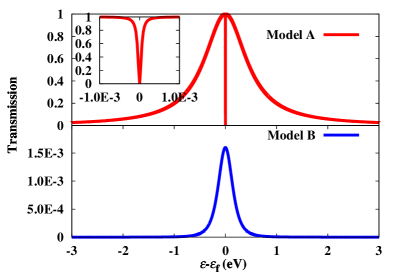
Figure 1: Transmission coefficient of models A and B. Comparison between the transmissions of the two models indicates the strong suppression of transmission due to the destructive quantum interference. The inset shows the transmission coefficient of model A near the Fermi level, which has very low transmission in this regime due to antiresonance.

Figure. 1 shows the transmission coefficient of the two models. Due to the destructive quantum interference effect, the transmission coefficient of model B is suppressed by at least 3 order of magnitude compared to that of model A. The suppression of transmission due to quantum interference effect in model B applies throughout the whole energy range, including resonant and off-resonant regime. The presence of destructive quantum interference effect in model B comes from the outgoing wave function associated with the tunneling process through state 2 to the right lead, which has $\pi$ phase difference from the tunneling through state 1 to the right lead. This phase difference arises from the different spatial structure of the two states and is indicated by the different sign of system-lead coupling strengths to right lead Härtle et al. (2013). In contrast to model B, model A differs from it by the sign of coupling strength between state 2 and right lead, i.e., $V_{R,2}$. As shown in Fig. 1, transmission of model A does not show destructive quantum interference effect except in a narrow range in $[\epsilon_{1}:\epsilon_{2}]$. The low transmission in this range is due to the antiresonance Bergfield and Stafford (2009).

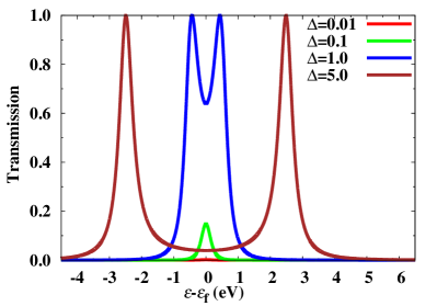
Figure 2: Transmission of model B with different energy gap ($\Delta$).

The energy gap between the two states ($\Delta=\epsilon_{2}-\epsilon_{1}$) is designed to be small compared to the line-width, i.e. $\Delta<\Gamma$, where $\Gamma=\sum_{\alpha}\Gamma_{\alpha}$. This is very similar to the optical interference of double-slit which requires the width of double-slit to be small compared to the light wavelength. If $\Delta\gg\Gamma$, electrons transport through the two states independently, quantum interference cannot be observed. Fig. 2 plots the transmission of model B with different energy gap. The transmission increases with increasing energy gap. At last, the transmission shows two conduction channels when $\Delta\gg\Gamma$, which indicates that quantum interference dims out with increasing energy gap.

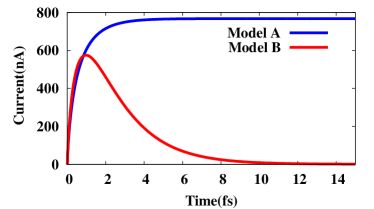
Figure 3: Transient currents of model A and B. The real-time dynamic of model B demonstrates the formation of destructive quantum interference effect, resulting in a very low state current when the interference is established. The time-dependent bias voltage is exponential growth type, $V_{L}(t)=-V_{R}(t)=V_{0}(1-e^{-t/a})$ where $V_{0}=5$ meV and $a=0.1$ fs.

Next, the dynamics of the two models under time-dependent bias voltage are examined. The systems are in equilibrium state before turning on bias voltage. After the time-dependent bias voltages are applied on the leads, the systems are driven out of equilibrium. In this study, the applied bias voltage is applied in a symmetric way: $V_{L}(t)=-V_{R}(t)=V_{0}(1-e^{-t/a})$ where $V_{0}=5$ meV and $a=0.1$ fs. The voltage is designed to be turned on quickly, i.e., $a<\hbar/\Gamma$, in order to ensure the time-scale of the dynamics is dominated by the intrinsic time-scale of the system itself. The transient currents of models A and B are represented in Fig. 3. As mentioned before, the life-time of the states is $\sim 1.3$ fs, transient current quickly reach its steady state in several femto-seconds. Compared to model A, transient current of model B shows similar behaviour at the very beginning after the turning on the bias voltage. It begins to deviate from model A after about 1 fs where quantum interference begins to take effect as electrons with $\pi$ phase difference reach the right lead. The $\pi$ phase difference is accumulated in the transport process from the two states to the right lead with increasing number of electrons reaching the right lead via the two states, resulting in more pronounced destructive quantum interference effect. As a consequence, the current of model B diminishes as approaching steady state.

Due to the destructive quantum interference effects, the transient current of model B reaches a rather low value ($\sim 1.2$ nA) in the steady state. It is about 3 order of magnitude smaller compared to the steady state current of model A, which is consistent with the difference between the transmissions of the two models shown in Fig. 1. The evolution of the transient current indicated by Fig. 3 clearly demonstrates the transient formation of quantum interference effect in the junctions, which requires a finite time to establish.

III.2 Dynamics of decoherence in presence of electron-phonon interaction

In the realistic devices, electron has the possibility of losing phase coherence through the scattering by phonon or other phase-breaking mechanism. In this section, the effects of electron-phonon coupling on quantum interference phenomena, i.e., decoherence dynamics, is examined. In this study, only a single vibrational mode is considered for simplicity. Besides, the phonon is assumed to only coupled to one of the states. The corresponding model is listed in the Table. 1 as model C.

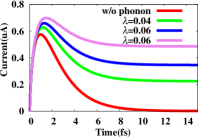
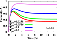
Figure 4: Transient currents of model C with different setups. Left panel: transient currents of four setups with different electron-phonon coupling constant; Right panel: transient currents of four setups with different phononic temperature. The time-dependent bias voltage is $V_{L}(t)=-V_{R}(t)=V_{0}(1-e^{-t/a})$, where $V_{0}=5$ meV and $a=0.1$ fs.

The quantum dynamics of model C are studied by applying a time-dependent bias voltage which is same as the non-interacting case. The system is initially in equilibrium state with electron-phonon interaction before turning on the bias voltage. Fig. 4 shows the transient currents of model C with different setups. On the left panel, transient currents with different electron-phonon coupling strength are demonstrated, the temperatures of leads and phonon are all set to be $T=0.0258$ eV, corresponding to the room temperature. It clearly shows that the introduction of electron-phonon interaction pronouncedly increases the steady state current, which is due to the decoherence in presence of phonon. Shortly after turning on the bias voltage, the four different setups show similar dynamics, this regime is related to the tunneling event of electrons from left lead to the two states. When electrons start to tunnel from the two states to right lead, transient currents begin to deviate. The reason is that the inelastic scattering by phonon partly destroys the phase coherence between the transport electrons. Stronger the electron-phonon coupling is, more electrons will be scattered by phonons and the coherence is further destroyed. As a result, the interference between the tunneling electrons from the two different states is significantly suppressed by phonon scattering, and steady state current shows monotonous relation with electron-phonon coupling strength as indicated in the left panel of Fig. 4.

The right panel of Fig. 4 shows the transient currents with different phononic temperature. The electron-phonon coupling constant is set as $\lambda=0.05$ eV. At higher temperature, more phonons are occupied and hence the probability of electrons being scattered is increased, and accordingly suppresses the quantum interference effect. Consequently, the current is enhanced by increasing the phononic temperature as indicated in the right panel of Fig. 4.

IV Summary

In this work, a dissipative time-dependent quantum transport theory in the strong electron-phonon interaction regime is established through the combination of TDDFT-OS-NEGF-WBL method and polaron transformation. The polaron transformation avoids the explicit electron-phonon coupling term, the effect of phonon on electron is transformed to the polaron shifted energies, phonon mediated effective electron-electron interaction and dressed device-lead coupling. In the high temperature limit, neglecting the difference between lesser and greater shift-generator correlation function results in a simple EOM formalism which terminates at the first tier similarly as the non interacting case. For the low temperature, second tier auxiliary density matrix arises, and corresponding EOMs are derived. It is worth noted that we demonstrate in this work the validity of TDDFT-OS with tight-binding model for simplicity. Since the formalism established in this work is based on single-particle theory, it can be readily implemented with TDDFT. Within TDDFT, the correlation-effect which is neglected in this work can also be taken into account through exchange-correlation functional.

The dissipative time-dependent quantum transport theory in the strong electron-phonon interaction regime is applied to study the quantum interference and phonon-induced decoherence in the molecular junctions. In absence of electron-phonon interaction, transient current of the interference model system clearly shows the transient effect of quantum interference, i.e. it undergoes a nonequilibrium process before the interference pattern is formed. The interference effect is reflected in the transient current of the system. Shortly after the turning on the bias voltage, the transient current increases before the interference effect is established. As the destructive interference pattern forms when electrons reach the right lead, it suppresses significantly the current. As a result, the transient current of quantum interference system presents an overshot in the initial trace and diminishes in the long time limit. The introduction of electron-phonon interaction scatters electrons when they transport through the junction. The scattering process breaks the phase coherence between electrons from the two different states. This decoherence effect due to electron-phonon scattering breaks the quantum interference effect, resulting in pronounced increase of current.