The role of currents distribution in general relativistic equilibria of magnetized neutron stars

Abstract

Magnetic fields play a critical role in the phenomenology of neutron stars. There is virtually no observable aspect which is not governed by them. Despite this, only recently efforts have been done to model magnetic fields in the correct general relativistic regime, characteristic of these compact objects. In this work we present, for the first time a comprehensive and detailed parameter study, in general relativity, of the role that the current distribution, and the related magnetic field structure, have in determining the precise structure of neutron stars. In particular, we show how the presence of localized currents can modify the field strength at the stellar surface, and we look for general trends, both in terms of energetic properties, and magnetic field configurations. Here we verify that, among other things, for a large class of different current distributions the resulting magnetic configurations are always dominated by the poloidal component of the current.

1 Introduction

The peculiar phenomenology of Anomalous X-Ray Pulsars (AXPs) and Soft Gamma Repeaters (SGRs) (Mereghetti, 2008), has led to the introduction of a new class of astrophysical sources, called magnetars (Duncan & Thompson, 1992; Thompson & Duncan, 1993). These are Neutron Stars (NSs) endowed with a very strong magnetic field $\sim 10^{14}-10^{15}$ G, about two orders of magnitude stronger than what is found in normal pulsars. This strong magnetic field is supposed to form at birth, involving possibly some form of dynamo action (Bonanno, Rezzolla & Urpin, 2003; Rheinhardt & Geppert, 2005). At birth the star is still fluid, and will remain so for a typical Kelvin-Helmoholtz timescale [$\sim 10-100$ s (Pons et al., 1999)], before the formation of a crust. This timescale is much longer than a typical Alfvén timescale, and one expects the magnetic field, in the end, to relax to some form of stable or meta-stable configuration (Braithwaite & Spruit, 2006; Braithwaite & Nordlund, 2006; Braithwaite, 2009).

It is well known that it is the magnetic field that dictates how NSs manifest themselves in the electromagnetic spectrum. In the astrophysical community, a vast effort has been devoted to model the outer magnetosphere of these objects, from the pioneering work of Goldreich & Julian (1969) to the most recent numerical models by Tchekhovskoy, Spitkovsky & Li (2013). This contrasts with the attention that has been placed on modeling the interior structure of these objects, which has been mostly driven by key fundamental questions of nuclear and theoretical physics. Most of the efforts in this respect have gone toward the study of their Equation of State (EoS) (Chamel & Haensel, 2008; Lattimer, 2012) and their cooling properties (Yakovlev & Pethick, 2004; Yakovlev et al., 2005).

When dealing with problems related to the EoS or the cooling, one can safely assume that the NS is spherically symmetric (which is a good approximation except for the fastest rotators). This greatly simplifies the equations that one needs to solve. On the other hand, it is obvious that the geometry of the magnetic field is, instead, a truly multidimensional problem. This means that, except for trivial cases, the task of finding equilibrium solutions can only be handled numerically. The techniques to model magnetic field in General Relativity, i.e. GR-MHD and its extensions (Font, 2008), have been mostly developed in the last 10-15 years. As a consequence, only recently attention has been paid to the study of magnetic field structure and evolution in NSs (Bocquet et al., 1995; Haskell et al., 2008; Konno, 2001; Kiuchi & Yoshida, 2008; Kiuchi, Kotake & Yoshida, 2009; Frieben & Rezzolla, 2012; Yazadjiev, 2012; Fujisawa, Yoshida & Eriguchi, 2012; Yoshida, Yoshida & Eriguchi, 2006; Ciolfi et al., 2009; Ciolfi, Ferrari & Gualtieri, 2010; Ciolfi & Rezzolla, 2013; Lander & Jones, 2009; Glampedakis, Andersson & Lander, 2012; Pili, Bucciantini & Del Zanna, 2014a, b; Armaza et al., 2014).

In general, these studies have focused on trying to obtain specific configurations, and on investigating a few key aspects of the field morphology. However, a detailed study of the parameter space is still partially lacking. This, obviously, raises questions about the robustness and generality of some conclusions. Moreover, it does not allow us to understand if there are general trends and expectations.

For this reason, in this paper we present a detailed parameter study in GR-MHD of currents distribution and the related magnetic field configurations in NSs. Extending, in part, the work done in Pili, Bucciantini & Del Zanna (2014a), we introduce several new functional forms for the current distribution, and investigate the properties of the resulting magnetic field. We show that there are general trends associated with the nonlinear behavior of currents, both in terms of global integrated quantities and for what concerns the structure of the magnetic field at the surface. We also show the interplay of various nonlinear terms, and address the robustness of several outcomes.

This paper is organized as follows. In Sect. 2 we introduce the formalism, and in particular in Sect. 2.2 the various functional forms used for the currents are discussed. In Sect. 3 we present our results, and finally conclude in Sect. 4.

2 The mathematical framework

Let us briefly describe here our mathematical framework, in particular the equations that are solved to derive the magnetic field equilibrium configurations, and the choices we have adopted in order to describe different magnetic geometries. For further details the reader is referred to Pili, Bucciantini & Del Zanna (2014a), where the full mathematical setup is presented. In the present work we will assume that the magnetic field strength is well below the energy equipartition value, so that the field does not affect neither the overall fluid configuration (assumed to be static and barotropic) nor the metric, as discussed in Pili, Bucciantini & Del Zanna (2014b). Thus, given a consistent spacetime metric and fluid configuration, we are going to see how to build a magnetic field configuration on top of it.

In the following we assume a signature $(-,+,+,+)$ for the spacetime metric. Quantities are expressed in geometrized units $c=G=1$, unless otherwise stated, and all $\sqrt{4\pi}$ factors are absorbed in the definition of the electromagnetic fields.

2.1 The Grad-Shafranov equation

The spacetime and matter distribution of a nonrotating NS, under the assumption of a negligible magnetic field, are spherically symmetric. In this case the spacetime is also conformally flat, and the line element can be written, using standard isotropic coordinates $(t,r,\theta,\phi)$, as

$${\rm d}s^{2}=-\alpha^{2}{\rm d}t^{2}+\psi^{4}({\rm d}r^{2}+r^{2}{\rm d}\theta^{2}+r^{2}\sin^{2}\!\theta\,{\rm d}\phi^{2}),$$ (1)

where $\alpha$ is the lapse function and $\psi$ is the conformal factor, which are functions only of the radial coordinate $r$. These metric terms are related to the matter distribution by two elliptic equations, derived from Einstein equations, namely

$$\Delta\psi=[-2\pi\psi^{5}e],$$ (2)

$$\Delta(\alpha\psi)=[2\pi(e+6p)\psi^{4}](\alpha\psi),$$ (3)

where $\Delta$ is the usual 3D Laplacian of flat spacetime, while $e$ and $p$ represent, respectively, the energy density and the pressure measured by the Eulerian observer. For a more general discussion in the case of rotation and/or a strong magnetic field see (Bucciantini & Del Zanna, 2011; Pili, Bucciantini & Del Zanna, 2014a, b).

For an axisymmetric configuration in a static spacetime, the electromagnetic field can be described uniquely in terms of a magnetic potential that coincides with the $\phi$-component of the vector potential $A_{\phi}$ , which is usually referred to as the magnetic flux function. In particular the solenoidality condition, together with axisymmetry, allows one to express the poloidal component of the magnetic field as the gradient of a magnetic flux function, whereas any toroidal component at equilibrium must be related to $A_{\phi}$ by means of a scalar current function $\mathcal{I}$, that depends on $A_{\phi}$ alone. Thus, the components of the magnetic field are given by

$$B^{r}=\frac{\partial_{\theta}A_{\phi}}{\psi^{6}r^{2}\sin\theta},\quad B^{\theta}=-\frac{\partial_{r}A_{\phi}}{\psi^{6}r^{2}\sin\theta},\quad B^{\phi}=\frac{\mathcal{I}(A_{\phi})}{\alpha\psi^{4}r^{2}\sin^{2}\theta},$$ (4)

for any choice of the free function $\mathcal{I}(A_{\phi})$. Notice that here we are implicitly assuming the presence of a nonvanishing poloidal component. In the case of purely toroidal magnetic field, on the other hand, the vector potential $A_{\phi}$ is not defined and a different approach must be adopted [see Pili, Bucciantini & Del Zanna (2014a) for details].

The Euler equation for a static and barotropic (the pressure is a function of rest mass density alone) GRMHD configuration can be written as

$$\partial_{i}\ln h+\partial_{i}\ln\alpha=\frac{{\rm d}\mathcal{M}}{{\rm d}A_{\phi}}\partial_{i}A_{\phi},$$ (5)

where $i=r,\theta$, leading to the magnetic Bernoulli-like integral

$$\ln{\left(\frac{h}{h_{\rm c}}\right)}+\ln{\left(\frac{\alpha}{\alpha_{\rm c}}\right)}-\mathcal{M}=0,$$ (6)

in which the label ${\rm c}$ refers to values at the centre of the NS. Here $\rho$ is the rest mass density, $h:=(e+p)/\rho$ is the specific enthalpy, and the Lorentz force has been written in terms of the gradient of the magnetization function $\mathcal{M}$, our second scalar function of $A_{\phi}$. In other words, if $J^{i}=\alpha^{-1}\epsilon^{ijk}\partial_{j}(\alpha B_{k})$ is the conduction current, then

$$\rho h\partial_{i}\mathcal{M}=\epsilon_{ijk}J^{j}B^{k}.$$ (7)

This implies that the current components can be expressed in terms of the functions $\mathcal{I}(A_{\phi})$ and $\mathcal{M}(A_{\phi})$ as

$$J^{r}=\alpha^{-1}B^{r}\frac{{\rm d}\mathcal{I}}{{\rm d}A_{\phi}},\quad J^{\theta}=\alpha^{-1}B^{\theta}\frac{{\rm d}\mathcal{I}}{{\rm d}A_{\phi}},\quad J^{\phi}=\rho h\,\frac{{\rm d}\mathcal{M}}{{\rm d}A_{\phi}}+\frac{\mathcal{I}}{\varpi^{2}}\frac{{\rm d}\mathcal{I}}{{\rm d}A_{\phi}},$$ (8)

where we have introduced the generalized cylindrical radius $\varpi:=\alpha\psi^{2}r\sin\!\theta$.

The magnetic flux function $A_{\phi}$ is related to the metric terms and the hydrodynamical quantities through the so-called Grad-Shafranov (GS) equation (Pili, Bucciantini & Del Zanna, 2014a):

$$\tilde{\Delta}_{3}\tilde{A}_{\phi}+\frac{\partial A_{\phi}\partial\ln(\alpha\psi^{-2})}{r\sin\theta}+\psi^{8}r\sin\!\theta\left(\rho h\frac{{\rm d}\mathcal{M}}{{\rm d}A_{\phi}}+\frac{\mathcal{I}}{\varpi^{2}}\frac{{\rm d}\mathcal{I}}{{\rm d}A_{\phi}}\right)=0$$ (9)

which is obtained by working out the derivatives of the magnetic field in Eq. (7). For convenience we introduced the regularized potential $\tilde{A}_{\phi}=A_{\phi}/(r\sin\theta)$, and the following differential operators

$$\tilde{\Delta}_{3}\!:=\!\Delta-\frac{1}{r^{2}\sin^{2}\!\theta}\!=\!\partial^{2}_{r}+\frac{2}{r}\partial_{r}+\frac{1}{r^{2}}\partial_{\theta}^{2}+\frac{1}{r^{2}\tan{\theta}}\partial_{\theta}-\frac{1}{r^{2}\sin^{2}\!\theta},$$ (10)

$$\partial f\partial g:=\partial_{r}f\partial_{r}g+\frac{1}{r^{2}}\partial_{\theta}f\partial_{\theta}g.$$ (11)

The GS equation, which governs the hydromagnetic equilibrium inside the star, can be also extended outside it, just by neglecting the term proportional to the rest mass density. In this case one recovers the force-free regime (Pili, Bucciantini & Del Zanna, 2014c).

2.2 The currents distribution

As anticipated, the purpose of this paper is to study the properties of various distributions of induction currents, and related magnetic field configurations, in order to derive general trends and to understand what parameter governs the key aspects of the magnetic field geometry. For this reason we have adopted functional forms for the free $\mathcal{M}(A_{\phi})$ and $\mathcal{I}(A_{\phi})$ functions allowing us to sample a large parameter space, and to investigate configurations with important morphological properties.

The magnetization function $\mathcal{M}$ has been chosen in order to include nonlinear terms in the form

$$\mathcal{M}(A_{\phi})=k_{\rm pol}A_{\phi}\left[1+\frac{\xi}{\nu+1}\left(\frac{A_{\phi}}{A_{\phi}^{\rm max}}\right)^{\nu}\right],$$ (12)

where $k_{\rm pol}$ is the poloidal magnetization constant, $\nu$ is the poloidal magnetization index of the nonlinear term, which is normalized to the maximum value of the vector potential itself $A_{\phi}^{\rm max}$. This normalization prevents the nonlinear term from diverging, and it allows the system to remain within the weak field limit. The magnetization function $\mathcal{M}$ vanishes outside the surface of the NS.

For the current function $\mathcal{I}$, we adopted either the form

$$\mathcal{I}(A_{\phi})=\frac{a}{\zeta+1}\Theta[A_{\phi}-A_{\phi}^{\rm sur}]\frac{(A_{\phi}-A_{\phi}^{\rm sur})^{\zeta+1}}{{(A_{\phi}^{\rm sur})}^{\zeta}},$$ (13)

or

$$\mathcal{I}(A_{\phi})=\frac{a}{\zeta+1}\Theta[A_{\phi}-A_{\phi}^{\rm sur}]\frac{(A_{\phi}-A_{\phi}^{\rm sur})^{\zeta+1}(A_{\phi}^{\rm max}-A_{\phi})^{\zeta+1}}{{(A_{\phi}^{\rm sur}A_{\phi}^{\rm max})}^{\zeta+1/2}},$$ (14)

where $\Theta[.]$ is the Heaviside function, $A_{\phi}^{\rm sur}$ is the maximum value that the $\phi$ component of the vector potential reaches on the stellar surface, $a$ is the toroidal magnetization constant and $\zeta$ is the toroidal magnetization index. In both cases the toroidal magnetic field is fully confined within the star. However, the first case corresponds to a Twisted Torus (TT) configuration, where the azimuthal current has the same sign over its domain and the toroidal field reaches its maximum where the poloidal field vanishes. On the other hand, the second case corresponds to a Twisted Ring (TR) configuration, where the current changes its sign, and the toroidal field vanishes in the same place where the poloidal field goes to zero.

With our normalization choices in Eqs. (12) (13) (14), the solution of the GS equation does not depend on the strength of the magnetic field. In the limit of a weak field, the metric and fluid quantities $\rho$, $h$, $\psi$, and $\alpha$ can be assumed as fixed, such that, if $A_{\phi}$ is a solution of the GS equation for given values of $k_{\rm pol},\xi,\nu,a,\zeta$, then $\eta A_{\phi}$ will be a solution of the GS equation for $\eta k_{\rm pol},\xi,\nu,a,\zeta$, for both TT and TR cases. Our solution can be thus renormalized to any value of the magnetic field strength. In particular we have chosen to display our solution by normalizing the strength of the magnetic field at the pole to $10^{14}$ G. We verified that the limit of a weak field holds to a high level of accuracy up to a maximum strength $\sim 10^{16}$ G, corresponding to a typical surface magnetic field $\sim$ a few $\times 10^{15}$ G (Pili et al. 2014 submitted). For higher fields, we observe non-linear variations in the ratios of magnetic quantities, higher than the overall accuracy of our scheme (see Sect. 2.3). A partial investigation of the strong field regime, for purely poloidal cases, is presented in Appendix B.

2.3 The numerical setup

In all our models we assume that the NS is described by a polytropic EoS $p=K_{\rm a}\rho^{\gamma_{\rm a}}$ (a special case of the general barotropic EoS $p=p(\rho)$), with an adiabatic index $\gamma_{\rm a}=2$. Unless otherwise stated, the polytropic constant is chosen to be $K_{\rm a}=110$ (in geometrized units). Given that we are here interested in studying different distributions of currents, in the limit of weak magnetic fields, we assume a fiducial model for the NS that is unaffected by the magnetic field itself, unless otherwise stated. The role of a strong field has been already investigated in a previous paper (Pili, Bucciantini & Del Zanna, 2014a).

The fiducial NS model used for computing, on top of it, the various magnetic field configurations, has a central rest mass density $\rho_{\rm c}=6.354\times 10^{14}\,\mbox{g}\,\mbox{cm}^{-3}$, a baryonic mass $M_{0}=1.500M_{\sun}$, a gravitational mass $M=1.400M_{\sun}$, and a circumferential radius $R_{\rm circ}=15.22\,\mbox{km}$ (corresponding to an isotropic radius $R_{\rm NS}=13.06\,\mbox{km}$). This fiducial model is computed in isotropic coordinates using the algorithms and the numerical scheme described in Bucciantini & Del Zanna (2011).

On top of this fiducial model we then solve the GS equation, Eq. (9), as described in Pili, Bucciantini & Del Zanna (2014a). Let us briefly recall here the main features of the algorithm employed. The GS equation is a nonlinear vector Poisson equation for the azimuthal component of the regularized potential $\tilde{A}_{\phi}$. The solution is searched in the form of a series of vector spherical harmonics

$$\tilde{A}_{\phi}(r,\theta):=\sum_{l=0}^{l_{\rm max}}[C_{l}(r)Y^{\prime}_{l}(\theta)],$$ (15)

where $Y_{l}(\theta)$ are the standard scalar spherical harmonics, the ^′ indicates derivation with respect to $\theta$, and we have used the axisymmetric assumption to exclude terms with $m\neq 0$. We want to stress here again that in the low magnetization limit one can safely assume that the metric and the matter distribution are unaffected by the magnetic field, then in the present approximation we only need to solve the GS equation, for any given fluid structure and associated spacetime metric.

Our algorithm allows us to solve the GS equation over the entire numerical domain including both the interior of the star and the surrounding magnetosphere where the rest mass density is numerically set to a fiducial small value ($\sim 10^{-6}$ times the value of the rest mass density at the centre of the star), without the need of a matching procedure between the exterior solution with the interior one. The threshold value for the rest mass density is chosen such that lowering it further produces negligible changes (much smaller than the overall accuracy of our scheme). We want also to point here that typical rest mass densities in the atmospheres of proto-NS are $\sim 10^{6}-10^{8}$ g cm^-3 (Thompson, Burrows & Meyer, 2001). This also guarantees smoothness of the solutions at the stellar surface, avoiding surface currents. Moreover, the harmonic decomposition ensures the correct behavior of the solution on the axis of symmetry, and the asymptotic trend of the radial coefficients $C_{l}(r)$ can be correctly imposed such that they go to 0 with parity $(-1)^{l}$ at the centre, and as $C_{l}(r)\propto r^{-(l+1)}$ at the outer boundary.

The decomposition in Eq. (15) reduces the GS equation to a system of radial 2nd-order elliptical nonlinear PDEs for the various coefficients $C_{l}(r)$. These are solved, using a direct tridiagonal matrix inversion (Bucciantini & Del Zanna, 2011; Pili, Bucciantini & Del Zanna, 2014a). The entire procedure is repeated until the solution converges with accuracy $\sim 10^{-8}$.

The numerical solutions presented here are always computed in a spherical domain covering the range $r=[0,22]$ and $\theta=[0,\pi]$. A uniform spherical grid is adopted with 700 points in the radial direction and 400 in the angular one. The harmonic decomposition of the vector potential has $l_{\rm max}=60$. We verified that the overall accuracy of the solutions is $\sim 10^{-3}$.

3 Numerical equilibrium models

3.1 Purely poloidal configurations

Let us begin by illustrating the properties of models with a purely poloidal field, obtained by a purely toroidal current with $\mathcal{I}=0$, so that all properties will be determined by the function $\mathcal{M}(A_{\phi})$ alone. As already pointed out in our previous paper (Pili, Bucciantini & Del Zanna, 2014a), the parity of the magnetic field with respect to the equator depends on the parity of the linear current term in the magnetization function $\mathcal{M}$. This is proportional to the rest mass density $\rho$, it is symmetric with respect to the equator, whereas the related magnetic field is antisymmetric. The nonlinear term cannot change this parity. The result is that all our models are dipole-dominated, and only terms odd in $l$ are present in Eq. (15). See Appendix A for a discussion on how one can obtain antisymmetric solutions.

The value of $\xi$ can be chosen such that the nonlinear term in Eq. (12), leads to subtractive currents ($\xi<0$) or additive currents ($\xi>0$), while the value of $\nu$ sets how much concentrated this current is.

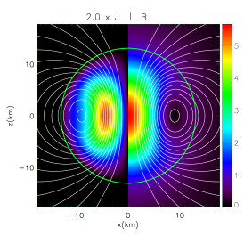
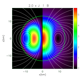
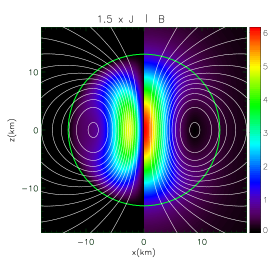
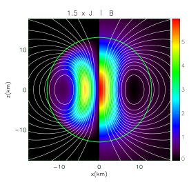
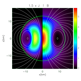
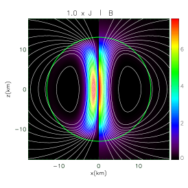
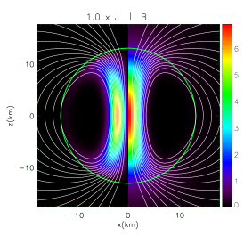
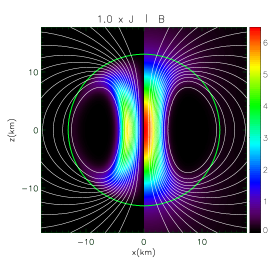
Figure 1: Purely poloidal field case. Strength of the azimuthal current in units of $10^{19}$G s^-1 (left half of each panel) and strength of the poloidal magnetic field in units $10^{14}$ G (right half of each panel). White contours represent magnetic field surfaces (isocontours of $A_{\phi}$). The left column represents cases with $\nu=1$, the central one those with $\nu=4$, the right one those with $\nu=10$. From top to bottom, rows represent cases with $\xi=-0.5,-0.9,-1.0$. The thick green line is the stellar surface. In all cases the surface magnetic field at the pole is $10^{14}$ G. Axes refer to a cartesian frame centered on the origin and with the $z$-axis corresponding to the symmetry axis.

In Fig. 1 we show the magnetic field and the current distribution for a series of models computed with different values of $\xi<0$ and different values for the poloidal index $\nu$. The effect of the nonlinear term is to suppress the currents in the outer part of the star, and to concentrate them in the inner region. The same holds for the magnetic field. As $\xi$ decreases, the interior of the star becomes progressively less magnetized, and the magnetic field is confined toward the axis. It is interesting to note that this effect becomes significative only as $\xi$ approaches $-1.0$ (for values of $\xi$ closer to $0$ deviations are marginal). Moreover it is evident that in the case of subtractive currents the magnetic field geometry that one finds is almost independent on the magnetization index $\nu$. Indeed the change in poloidal index seems only to produce marginal effects in the magnetic field distribution, with configurations that are slightly more concentrated toward the axis for smaller values of $\nu$. In particular we find that the unmagnetized and current free region extends to fill the outer half of the star (the magnetic field at the equator drops to zero at about half the stellar radius). One also finds, in general, that the ratio of the strength of the magnetic field at the pole, with respect to the one at the centre increases by about 30 to 50%, as $\xi$ approaches $-1$.

Interestingly, we were not able to obtain models with $\xi<-1$. This implies that we cannot find configurations where there is a current inversion (the sign of the current is always the same inside the star). Our relaxation scheme for the GS equation seems at first to converge to a metastable equilibrium with accuracy $\sim 10^{-4}$, but then the solution diverges. We want to stress here that the Grad-Shafranov equation, in cases where the currents are nonlinear in the vector potential $A_{\phi}$, becomes a nonlinear Poisson-like equation, that in principle might admit multiple solutions and bifurcations (local uniqueness is not guaranteed). This is a known problem (Ilgisonis & Pozdnyakov, 2003), and suggests that a very small tolerance (we adopt $10^{-8}$) is required to safely accept the convergence of a solution. This issue might be related to the problem of local uniqueness for nonlinear elliptical equations. It is well known that the nonlinear Poisson equations of the kind $\nabla^{2}\psi=k\psi^{a}$ satify local uniqueness only if $ka\geq 0$. It is evident that this depends on the relative sign of the coefficient and exponent of the nonliner source term: in our case the relative sign of $\xi$ and $\nu$. Given that $\nu$ is always positive, what matters is just the sign of $\xi$. This explains why we can obtain solutions with additive currents ($\xi>0$) even in the regime dominated by the nonlinear term, while solutions with subtractive currents ($\xi<0$) can only be built up to $\xi>-1$, where the contribution of the nonlinear current is still smaller than the linear one which act as a stabilizing term. However we want to recall here that the Grad-Shafranov is not a Poisson equation, and it is not proved that the same uniqueness criteria apply.

In Fig. 2 we show the opposite case of additive currents, $\xi>0$. The value of $\nu$ in this case establishes how much concentrated these currents are, and plays a major role in determining the properties of the resulting magnetic field. Rising the value of $\xi$ the nonlinear currents become progressively more important. We can define a nonlinear dominated regime in the limit of high $\xi$, where the magnetic field structure and distribution converge to a solution that is independent of $\xi$. The values of $\xi$, at which this limit is reached, depends on $\nu$. For $\nu=1$ the limit is achieved already at $\xi=20$ as can be inferred from Fig. 2, while for $\nu=10$ the limit is reached at $\xi\sim 1000$. As already noted (Pili, Bucciantini & Del Zanna, 2014a), in the case $\nu=1$ the presence of a nonlinear current term does not alter significantly the geometry of the magnetic field, or other global integrated quantities like the net global dipole moment. The ratio of the strength of the magnetic field at the centre with respect to the one at the pole diminishes slightly by about 10%. The location of the neutral current point, where the magnetic field vanishes is unchanged.

At higher values of $\nu$ the magnetic field geometry in the nonlinear dominated regime changes substantially. The overall current is strongly concentrated around the neutral point. The location of the neutral point itself shifts toward the surface of the NS, from about 0.7 stellar radii at $\xi=0$ to about 0.8 stellar radii in the nonlinear dominated limit. Moreover the maximum in the strength of the magnetic field is not reached at the centre any longer, but at intermediate radii where the nonlinear current is located. In this case the value of this local maximum can be a factor a few higher than the value at the centre. Configurations with two local maxima are also possible. This behavior is strongly reminiscent of what is found for the so-called TT configurations, where a toroidal component of the magnetic field is also present, inducing a current that behaves as the nonlinear term we have introduced here (see next section).

One can also look at the strength and distribution of the surface magnetic field, shown in Fig. 3. For decreasing values of $\xi<0$ the magnetic field tends to concentrate at the pole, in a region that is $\sim 30^{\circ}$ for $\xi=-1$. The radial magnetic field in the equatorial region is strongly suppressed, the field is almost parallel to the stellar surface, and the overall strength of the poloidal field is a factor 10 smaller with respect to the case with $\xi=0$ . In general these results are weakly dependent on the value of $\nu$, with higher values of $\nu$ leading to configurations where the field is slightly less concentrated toward the poles. A quite different behavior is seen for the cases of additive currents $\xi>0$. For $\nu=1$, the radial component of the magnetic field tends to be higher than in the case $\xi=0$, and it tends to be uniform in the polar region. The $\theta$ component of the magnetic field increases in the equatorial region by about a factor 2. The overall strength of the magnetic field becomes quite uniform over the stellar surface in the nonlinear dominated regime. These effects are further enhanced for increasing values of $\nu$. At $\nu=4$, in the nonlinear dominated regime, the radial component of the magnetic field reaches its maximum at $\sim\pm 25^{\circ}$ from the equator. The $\theta$ component, parallel to the NS surface, is instead strongly enhanced by about a factor 3 at the equator. The result is that for increasing $\xi$ there is a transition from configurations where the poloidal field strength is higher at the poles, to configurations where it is higher (by about 40%) at the equator, with intermediate cases where it can be almost uniform. At $\nu=10$ these effects are even stronger: the radial field now peaks very close to the equator, at $\sim\pm 10^{\circ}$, and the overall strength of the magnetic field can be higher at the equator by a factor $\sim 3$ with respect to the poles. This is the clear manifestation of a concentrated and localized peripheral current, close to the surface of the star.

To summarize the results in the fully saturated non-linear regime:

• subtractive currents, independent of their functional form, confine the magnetic field toward the axis, leaving large unmagnetized region inside the star;

• for subtractive currents, the surface magnetic field is concentrated in a polar region of $\sim 30^{\circ}$ from the pole, while at lower latitudes ($\pm 40^{\circ}$ from the equator) it can be a factor 10 smaller than at the pole (to be compared with one half for pure dipole);

• additive currents tend to concentrate the field in the outer layer of the star, the effect being stronger for higher values of the non-linearity; the field strength reaches its maximum closer to the surface, while its strength at the center can be even more than a factor 2 smaller;

• for additive current, the structure of the field at the equator can be qualitatively different than a dipole: higher at the equator than at the pole, even by a factor a few. A geometry similar to what is found in TT configurations.

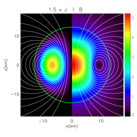
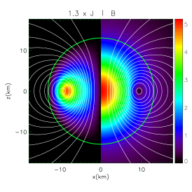
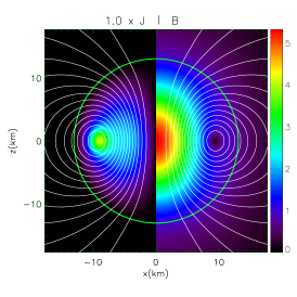
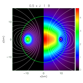
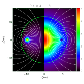
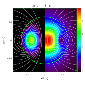
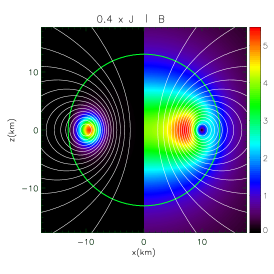
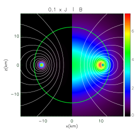
Figure 2: Purely poloidal field case. Strength of the azimuthal current in units of $10^{19}$G s^-1 (left half of each panel) and strength of the poloidal magnetic field in units $10^{14}$ G (right half of each panel). White contours represent magnetic field surfaces (isocontours of $A_{\phi}$). The left column represents cases with $\nu=1$, the central one those with $\nu=4$, the right one those with $\nu=10$. From top to bottom, rows represent cases with $\xi=2.0,10.0,200.0$. The thick green line is the stellar surface. In all cases the surface magnetic field at the pole is $10^{14}$ G. Axes refer to a cartesian frame centered on the origin and with the $z$-axis corresponding to the symmetry axis.

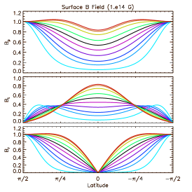
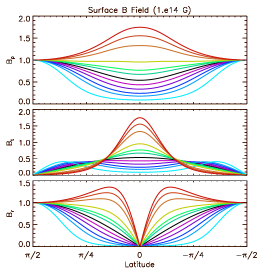
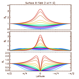
Figure 3: Purely poloidal field case. Magnetic field at the surface normalized to the value at the pole, for various values of $\xi$. Left column represents cases with $\nu=1$, central column cases with $\nu=4$ and right column cases with $\nu=10$. Upper panels display the total strength of the poloidal magnetic field, middle panels the strength of the parallel $\theta$ component, and lower panels the radial one.

3.2 Twisted Torus Configurations

Mixed geometries with poloidal and toroidal magnetic fields have been presented in the past in the so-called TT configurations (Ciolfi et al., 2009; Ciolfi, Ferrari & Gualtieri, 2010; Ciolfi & Rezzolla, 2013; Lander & Jones, 2009; Glampedakis, Andersson & Lander, 2012; Fujisawa, Yoshida & Eriguchi, 2012; Pili, Bucciantini & Del Zanna, 2014a, b). These configurations are characterized by a torus-like region, in the interior of the star, just under the stellar surface, where the toroidal field is confined. This geometry can be obtained if one chooses for the current function $\mathcal{I}$ the form of Eq. (13). In Fig.4 we show the magnetic field distribution for a typical TT solution.

Particular attention has been recently devoted to the study of this kind of systems, because there is evidence that magnetic field, in a fluid star, tends to relax toward a TT geometry, and that only mixed configurations can be dynamically stable (Braithwaite, 2009; Braithwaite & Nordlund, 2006; Braithwaite & Spruit, 2006). Motivated by these dynamical studies, efforts in the past have gone toward modeling systems where the equilibrium magnetic geometry was such that the magnetic energy was dominated by the toroidal component. Despite several attempts in various regimes (Ciolfi et al., 2009; Lander & Jones, 2009; Pili, Bucciantini & Del Zanna, 2014a), only configurations where the energetics was dominated by the poloidal component could be found. Recently Ciolfi & Rezzolla (2013) (CR13 hereafter) have shown that a very peculiar current distribution might be required in order to obtain toroidally dominated systems. This raises questions about the importance of the specific choice in the form of currents $\mathcal{I}$ and $\mathcal{M}$. More precisely one would like to know if previous failure to get toroidally dominated geometries is due to a limited sample of the parameter space, or if only very ad hoc choices for the current distribution satisfy this requirement. Moreover most of the efforts have concentrated onto understanding how this magnetic field acts on the star, and the amount of deformation that it induces. This is mostly motivated by searches for possible gravitational waves from neutron stars. Attention has focused on a limited set of models, and current distributions. In particular a deep investigation has been carried out only for the case $\zeta=0$ and $\zeta=0.1$ (Lander & Jones, 2009; Pili, Bucciantini & Del Zanna, 2014a).

Here we present a full investigation of TT configurations for various values of the parameter $\zeta$. This parameter regulates the shape of the current distribution inside the torus. For $\zeta\rightarrow-0.5$ the current becomes uniformly distributed within the torus, while for $\zeta>0$ it concentrates in the vicinity of the neutral line, where the poloidal field vanishes. It was shown that it is the integrated current associated with the current function $\mathcal{I}$ that prevents TT configurations to reach the toroidal dominated regime. As the strength of this current increases, the toroidal field rises, but the torus-like region shrinks toward the surface of the star and its volume diminishes.

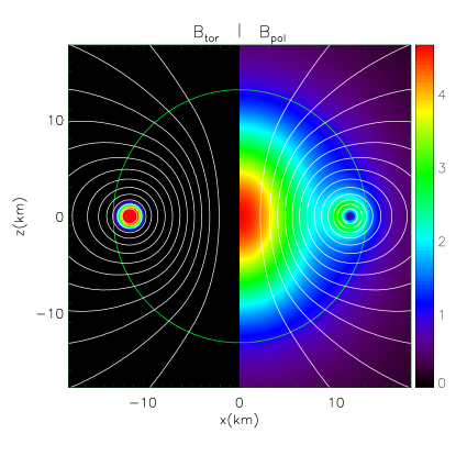
Figure 4: Magnetic field for a TT configuration with $\zeta=0$ and $a=1.5$ (corresponding to the maximum of the ratio $\mathcal{H}_{\rm tor}/\mathcal{H}$). Strength of the toroidal magnetic field (left), and poloidal magnetic field (right) normalized to the surface value at the pole. White contours represent magnetic field surfaces (isocontours of $A_{\phi}$). The thick green line is the stellar surface. Axes refer to a cartesian frame centered on the origin and with the $z$-axis corresponding to the symmetry axis.

In Fig. 5 we show how the ratio of magnetic energy associated to the toroidal field $\mathcal{H}_{\rm tor}$ over the total magnetic energy $\mathcal{H}$ changes with the parameter $a$ and $\zeta$. The maximum value of this ratio is always of the order of 0.06, slightly higher for smaller values of $\zeta$. In all cases we verified that at high values of $a$ the volume of the region containing the toroidal magnetic field is strongly reduced. For $\zeta=1$ we could not find equilibrium models (solution of the GS equation) all the way to the maximum (the algorithm failed to converge). Given that, for Eq. (13), both the energy of toroidal magnetic field and the associated current scale with $\mathcal{I}$, one cannot increase one without increasing the other. The systems seem always to self-regulate, with a maximum allowed current, implying a maximum allowed toroidal magnetic energy. The value of $\zeta$ affects the local value and distribution of the magnetic field, but does not play a relevant role for integrated quantities like currents and magnetic energy. Indeed by looking at Fig. 5, and Fig. 6, it is evident that for $\zeta<0$ it is not possible to have configurations where the maximum strength of the toroidal field exceeds the one of the poloidal field. For smaller $\zeta$ the same toroidal magnetic field energy, corresponds in general to weaker toroidal magnetic fields. For $\zeta>0$ instead we could reach configurations with a toroidal field stronger than the poloidal one. Interestingly the volume of the torus, for configurations where the ratio $\mathcal{H}_{\rm tor}/\mathcal{H}$ is maximal, does not depend on $\zeta$.

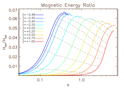
Figure 5: Value of the ratio $\mathcal{H}_{\rm tor}/\mathcal{H}$ for TT sequences characterized by different values for $\zeta$ as a function of $a$. The dashed lines correspond to configurations where the ratio between the maximum strength of the toroidal magnetic field $B_{\rm tor}^{\rm max}$, and the maximum strength of the poloidal component $B_{\rm pol}^{\rm max}$ is constant. From bottom to top $B_{\rm tor}^{\rm max}/B_{\rm pol}^{\rm max}=0.1,0.2,0.3,0.4,0.5,0.6,0.8,1.0,1.25$.

One can also look at the magnetic field distribution on the surface of the star. Given our previous results for purely poloidal configurations with nonlinear current terms, we expect strong deviations from the standard dipole, where the strength of the magnetic field at the pole is twice the one at the equator. In Fig. 6 we show the total strength of the magnetic field at the surface (where the field is purely poloidal), for configurations where the ratio $\mathcal{H}_{\rm tor}/\mathcal{H}$ is maximal. The presence of a current torus, just underneath the surface, is evident in the peak of the field strength at the equator. The peak is even narrower than what was found for purely poloidal cases with $\xi=10$, and the strength of the equatorial field can be more than twice the polar one. Again, there is little difference among cases with different $\zeta$. Higher values of $\zeta$ correspond to currents that are more concentrated around the neutral line, located at $\sim 0.85R_{\rm NS}$, and as such buried deeper within the star. Indeed the strength of the magnetic field at the equator with respect to the value at the pole, is higher for smaller $\zeta$.

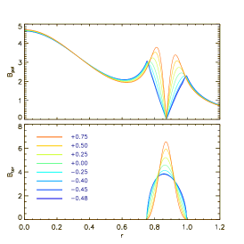
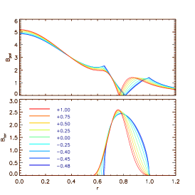
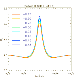
Figure 6: Left panel: strength of the poloidal magnetic field (top) and toroidal magnetic field (bottom) inside the star, on the equatorial plane, as a function of $r$, normalized to $R_{\rm NS}$, for models corresponding to the maximum of $\mathcal{H}_{\rm tor}/\mathcal{H}$, for various values of $\zeta$. Middle panel:strength of the poloidal magnetic field (top) and toroidal magnetic field (bottom) inside the star, on the equatorial plane, as a function of $r$, for models corresponding to $B_{\rm tor}^{\rm max}/B_{\rm pol}^{\rm max}=0.5$. Right panel: strength of the magnetic field at the surface for models corresponding to the maximum of $\mathcal{H}_{\rm tor}/\mathcal{H}$. In all cases the strength is normalized to the surface value at the pole.

Recently CR13 have presented results where the ratio $\mathcal{H}_{\rm tor}/\mathcal{H}$ is $>0.5$ and can reach value close to unity. However, in all of our models we get values $\mathcal{H}_{\rm tor}/\mathcal{H}$ always less than 0.1.

A precise comparison with CR13, is non trivial. For example, using the definition of current in their Eq.3, does not lead to converged solutions in the purely poloidal case (confirmed by Ciolfi, private communication). This because their formulation of Eq.3, with a non-linear term which introduces a subtractive currents with respect to the linear one, can lead to current inversions inside the NS. As we pointed out, our algorithm fails (diverges) every time we attempt to model systems with current inversions, and this might be related with uniqueness issue of the elliptical Grad-Shafranov equation. If this is indeed an issue with uniqueness then different numerical approaches might be more or less stable, and the robustness of the solution becomes questionable.

Note that CR13 impose that the field at the surface is a pure dipole, setting all other multipoles to zero. This might probably filter out and suppress the formation of localized currents at the edge of the NS and any effect associated to small scale structures, like the increase of the value of $A^{\phi}_{sur}$. As we show in this paper, the structure of the magnetic field at the surface, can dramatically differ from a pure dipole, depending on the current distribution. Even using the functional form by CR13, in the range where our code converges, we found that at the surface of the NS the magnetic field is far from a pure dipole.

Imposing a purely dipolar field outside the stellar surface may have been determinant in the results of CR13, but because we are not able to impose such a boundary condition, further independent verification is needed to resolve this issue.

3.3 Twisted Ring Configurations

In the previous section we have shown that in the case of TT geometry it is not possible to reach toroidally dominated configurations. This result is also independent on the particular shape of the current distribution $\mathcal{I}$. The system always self-regulates. As was pointed out by CR13 this is due to the one to one correspondence between integrated quantities, like the net current and magnetic field energy. Motivated by this, we can look for different forms for the equation $\mathcal{I}$ that allow a larger toroidal field, with a smaller net integrated current. The current given by Eq. (13) has always the same sign, and as shown, acts as an additive term. On the other hand, the current associated to Eq. (14) changes its sign within the toroidal region where it is defined. The field in this case has a geometry reminiscent of a Twisted Ring TR: its strength vanishes on the neutral line, where also the poloidal field goes to zero, and reaches a maximum in a shell around it. This can be clearly seen in Fig. 7. The net integrated currents in this case, is much less than in the case of Eq. (13), and it is globally subtractive.

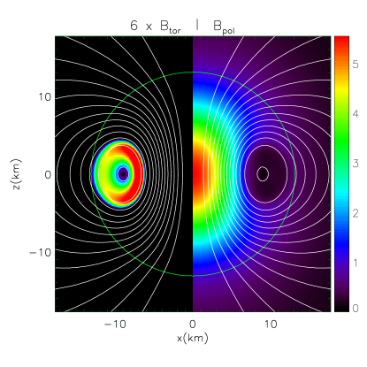
Figure 7: Magnetic field for a TR configuration with $\zeta=0$ and $a=12.6$ (corresponding to a ratio $B_{\rm tor}^{\rm max}/B_{\rm pol}^{\rm max}=0.15$ close to the maximum). Strength of the toroidal magnetic field (left) multiplied times a factor 6 for convenience, and poloidal magnetic field (right) normalized to the surface value at the pole. White contours represent magnetic field surfaces (isocontours of $A_{\phi}$). The thick green line is the stellar surface. Axes refer to distances in a cartesian frame centered on the origin and with the $z$-axis corresponding to the symmetry axis.

In Fig. 8 we show how the ratio of magnetic energy associated to the toroidal field $\mathcal{H}_{\rm tor}$ over the total magnetic energy $\mathcal{H}$ changes with the parameter $a$ and $\zeta$. Again we find that it is not possible to build models that are toroidally dominated. The maximum value of the ratio $\mathcal{H}_{\rm tor}/\mathcal{H}$ never exceeds 0.03 for all the values of $\zeta$ that we have investigated. The reason now is exactly the opposite of the one for TT configurations. The current of TR geometry, as anticipated, is subtractive. It acts like the nonlinear terms in the purely poloidal configurations with $\xi<0$. Its effect is to remove current from the interior of the star. This means that in the region where $\mathcal{I}\neq 0$, the vector potential $A_{\phi}$ becomes shallower: the quantity $[A_{\phi}^{\rm max}-A_{\phi}^{\rm sur}]$ diminishes. However, the strength of the toroidal magnetic field itself scales as $[A_{\phi}^{\rm max}-A_{\phi}^{\rm sur}]$. The nonlinearity of the problem manifests itself again as a self-regulating mechanism. Increasing $a$, in principle, implies a higher subtractive current, but this reduces the value of $[A_{\phi}^{\rm max}-A_{\phi}^{\rm sur}]$, and the net result is that subtractive current saturates, and the same holds for the toroidal magnetic field. This saturation is reached at small values of $\mathcal{H}_{\rm tor}/\mathcal{H}$. Indeed, in Fig. 8, a clear maximum is only visible for $\zeta<0$, while for $\zeta\geq 0$ the curves seem to saturate to an asymptotic value. Again we find that the value of $\zeta$ leads to small variations, with higher values of $\zeta$ leading to configurations with slightly higher value of $\mathcal{H}_{\rm tor}/\mathcal{H}$.

In all the parameter space we have investigated the strength of the toroidal magnetic field never exceeds the one of the poloidal component. At most, the toroidal magnetic field reaches values that are $\sim 0.15$ times the maximum value of the poloidal field. This is in sharp contrast with what was found for TT cases. Moreover, while in the TT cases the maximum strength of the toroidal field $B_{\rm tor}^{\rm max}$ was found to be a monotonically increasing function of the parameter $a$, along sequences at fixed $\zeta$, now $B_{\rm tor}^{\rm max}$ reaches a maximum $\sim 0.15B_{\rm pol}^{\rm max}$, and then slowly diminishes, as can be seen from Fig. 8. This is again a manifestation of the effect of subtractive currents. Interestingly, the region occupied by the toroidal magnetic field does not shrink as $a$ increases. The saturation of the toroidal magnetic energy is not due to a reduction of the volume filled by the toroidal field, but to a depletion of the currents.

As was done for the TT cases, we can also look at the distribution of magnetic field inside the star. In Fig. 9, we show the strength of the poloidal and toroidal components of the magnetic field along an equatorial cut. The effect of subtractive currents is evident in the suppression of the poloidal field in the TR region that extends from about half the star radius to its outer edge. It is also evident that the value of $\zeta$ plays only a minor role, and that differences are stronger at saturation than for intermediate values. Interestingly, there are very marginal effects concerning the strength of the magnetic field at the surface, which is essentially the same as the standard dipole. Again this can be partially understood recalling the behaviour of purely poloidal configurations with $\xi<0$. In those cases, substantial deviations from the dipolar case were achieved only in the limit $\xi\rightarrow 1$, when a large part of the star was unmagnetized. Here the size of the unmagnetized ring region remains more or less constant, and it does not affect the structure of the field at the surface. The global effect of the subtractive currents is small, and this reflects in the trend of the magnetic dipole moment, which diminishes only slightly by about 30-40%.

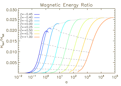
Figure 8: Value of the ratio $\mathcal{H}_{\rm tor}/\mathcal{H}$ for TR sequences characterized by different values for $\zeta$ as a function of $a$. The dashed lines correspond to configurations where the ratio between the maximum strength of the toroidal magnetic field $B_{\rm tor}^{\rm max}$, and the maximum strength of the poloidal component $B_{\rm pol}^{\rm max}$ is constant. From bottom to top $B_{\rm tor}^{\rm max}/B_{\rm pol}^{\rm max}=0.05,0.075,0.10,0.125,0.150$. The dotted line corresponds to configurations where $B_{\rm tor}^{\rm max}/B_{\rm pol}^{\rm max}=0.14$, indicating that the ratio of the magnetic field component is not monotonic.

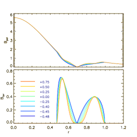
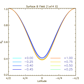
Figure 9: Left panel: strength of the poloidal magnetic field (top) and toroidal magnetic field (bottom) inside the star, on the equatorial plane, as a function of $r$, normalized to $R_{\rm NS}$,for models corresponding to the maximum of $\mathcal{H}_{\rm tor}/\mathcal{H}$, for various values of $\zeta$. Middle panel:strength of the poloidal magnetic field (top) and toroidal magnetic field (bottom) inside the star, on the equatorial plane, as a function of $r$, for models corresponding to $B_{\rm tor}^{\rm max}/B_{\rm pol}^{\rm max}=0.5$. Right panel: strength of the magnetic field at the surface for models corresponding to the maximum of $\mathcal{H}_{\rm tor}/\mathcal{H}$. In all cases the strength is normalized to the surface value at the pole.

3.4 Dependence on the stellar model

In the previous sections we have investigated in detail the role of two families of currents $\mathcal{I}$, that can be considered quite representative of a large class of current configurations. Our results show that in neither case we could obtain magnetic field distributions where the energetics was dominated by the toroidal component.

In this section we try to investigate the importance of the underlying stellar model. In general, previous studies have mainly focused on the distribution of currents, assuming a reference model for the NS: either a $1.4M_{\odot}$ (Ciolfi et al., 2009; Ciolfi, Ferrari & Gualtieri, 2010; Ciolfi & Rezzolla, 2013; Lander & Jones, 2009) or a $1.5M_{\odot}$ (Pili, Bucciantini & Del Zanna, 2014a) NS. Only Glampedakis, Andersson & Lander (2012) have partly investigated how the stellar structure might affect the energetics properties of the magnetic field. In particular they focused on the role of stable stratification, and showed that this might change the maximum amount of magnetic energy associated to the toroidal magnetic field, in standard TT configurations.

In Fig. 10 we show how the ratio $\mathcal{H}_{\rm tor}/\mathcal{H}$ changes as a function of $a$ for standard TT models with $\zeta=0$, but for NSs with different masses. For $K_{\rm a}=110$ the maximum mass for a NS is found to be $\sim 1.7M_{\odot}$. It is clear that models with a higher mass have a higher value of the ratio $\mathcal{H}_{\rm tor}/\mathcal{H}$ , for the same value of $a$. Interestingly, the maximum value reached by $\mathcal{H}_{\rm tor}/\mathcal{H}$ for a $1.7M_{\odot}$ NS, is about 0.08, compared to 0.06 for a $\sim 1.4M_{\odot}$ NS. This is a substantial relative increase, even if the magnetic energy is still dominated by the poloidal component. Moreover this increasing trend is stronger at higher masses.

We also investigated how much of this trend is related just to the total stellar mass (i.e. the compactness of the system) and how much depends on the value of rest mass density in the core of the NS. Indeed it was previously found the NSs with higher masses can harbor in principle stronger magnetic fields (Pili, Bucciantini & Del Zanna, 2014a). On the other hand, the current associated with $\mathcal{M}$, responsible for the structure of the poloidal field, scales as the rest mass density. For models built by keeping constant $K_{\rm a}=110$, a higher mass implies a higher central rest mass density, so that it is hard to disentangle them. In Fig. 10 we show also two models with different EoS: one that has the same central rest mass density as the $1.7M_{\odot}$ NS, but different values of the adiabatic constant $K_{\rm a}$, such that is total gravitational mass is $2.0M_{\odot}$; the other has the same mass of $1.7M_{\odot}$, but a lower central rest mass density (about one third). It is evident that models with a smaller total mass, given the same central rest mass density, correspond to lower maximum value for $\mathcal{H}_{\rm tor}/\mathcal{H}$. On the other hand, given the same central rest mass density, the ratio $\mathcal{H}_{\rm tor}/\mathcal{H}$ clearly increases with total mass. It appears that the rest mass density stratification (how much concentrated is the rest mass density distribution in the core and how much shallow is it in the outer layers), regulates the relative importance of $\mathcal{I}$ and $\mathcal{M}$, and the net outcome in terms of energetics of the toroidal and poloidal components.

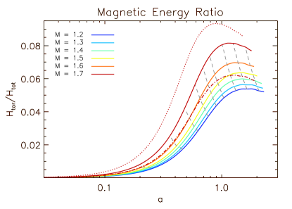
Figure 10: Value of the ratio $\mathcal{H}_{\rm tor}/\mathcal{H}$ for TT sequences with $\zeta=0$, characterized by different values for the gravitational mass as a function of $a$. The dashed grey lines corresponds to configurations where the ratio between the maximum strength of the toroidal magnetic field $B_{\rm tor}^{\rm max}$, and the maximum strength of the poloidal component $B_{\rm pol}^{\rm max}$ is constant. From bottom to top $B_{\rm tor}^{\rm max}/B_{\rm pol}^{\rm max}=0.1,0.2,0.3,0.4,0.5,0.6,0.8,1.0,1.25$. The dotted red line corresponds to a configuration with $M=2.0M_{\odot}$, and the same central rest mass density as the $1.7M_{\odot}$ case. The dot-dashed red line corresponds to a configuration with $M=1.7M_{\odot}$, but a lower central rest mass density with respect to the $K_{\rm a}=110$ case.

3.5 Mixed nonlinear currents

It was suggested by CR13 that a possible reason why TT configurations, computed using $\xi=0$ in $\mathcal{M}$, could not achieve the toroidally dominated regime, was due to the fact that the contribution to the azimuthal current from $\mathcal{I}$ soon dominates. As a consequence, the resulting poloidal configuration enters the nonlinear regime in which the size of the torus region, where the toroidal field is confined, shrinks. They show that, by introducing a current term in $\mathcal{M}$ to compensate for $\mathcal{I}$, it was possible to avoid this behaviour. However they also stressed the fact that a very peculiar form for $\mathcal{M}$ was needed to achieve significative results.

Here we investigate what happens to TT models, using for $\mathcal{I}$ the form of Eq. (13), if we retains nonlinear terms in the definition of $\mathcal{M}$, and what happens in cases where $\xi\neq 0$. In Fig. 11 we show how $\mathcal{H}_{\rm tor}/\mathcal{H}$ changes for TT configurations with $\zeta=0$ for various values of the parameter $\xi$ and for selected values of $\nu=1,4,10$. Naively, based on the idea that compensating currents are needed to achieve toroidally dominated configurations, one would expect that higher values of $\mathcal{H}_{\rm tor}/\mathcal{H}$ should be reached for $\xi<0$ (subtractive currents). Fig. 11 shows instead that the trend is the opposite. In general, lower values of $\mathcal{H}_{\rm tor}/\mathcal{H}$ are found for $\xi<0$ and higher for $\xi>0$, even if this is just a minor difference. The value of $\nu$ seems not to play a major role. Interestingly the effect is maximal for intermediate values of $\nu=4$, and marginal for $\nu=10$.

This counterintuitive trend is due to the fact that both the effects of the current term $\mathcal{I}$ and the contribution of nonlinear terms in $\mathcal{M}$, become important only in the fully nonlinear regime. For values of $\xi\sim 0$ the effect of the nonlinear current term in $\mathcal{M}$ is negligible. For higher values of $\xi$ this nonlinear term becomes more important. In the case $\xi<0$ they give rise to a compensating current (the net dipole grows less) but, as discussed, they also tend to suppress the vector potential and this effect is stronger, leading to a overall decrease of the magnetic field. In the case $\xi>0$, one would expect this additive current to lead to an even more pronounced reduction in the torus volume, however, this is not so. The net dipole increases but this additive currents enhance the vector potential and the net result is a higher $\mathcal{H}_{\rm tor}/\mathcal{H}$ (up to 30% higher for $\nu=4$ and $\xi=20$). The highly nontrivial behaviour of the nonlinear regime is apparent. It is however possible that different forms for the compensating current might lead to different results.

Interestingly, again we are not able to construct equilibrium model with current inversion. It is possible, for higher values of $\nu$, to build models with $\xi<-1$, but only as long as the current in the domain is always of the same sign. Indeed, cases with $\xi<-1$ are allowed by the presence of a current due to $\mathcal{I}$, given by Eq. (13), that is always additive. There appears to be a threshold value for $a$ below which cases with $\xi<-1$ are not realized. This is consistent with the argument about local uniqueness we discuss in the purely poloidal case. Solutions with subctractive currents can be built only as long as the nonlinear current term is subdominant, and other currents enforce stability. Given the presence of an extra current due to $\mathcal{I}$, associated with the toroidal magnetic field, now it is possible to build solutions with $\xi<-1$.

Similar results apply for the cases of TR configuration where $\mathcal{I}$ is given by Eq. (14). In Fig. 12 we show these results. For values of $\xi<0$ the ratio $\mathcal{H}_{\rm tor}/\mathcal{H}$ is essentially unchanged (it looks like the ratio is marginally smaller). For positive values of $\xi$ we found a substantial increase: $\mathcal{H}_{\rm tor}/\mathcal{H}$ can be a factor 2 higher than in the simple TR case. In this case, the additive non linear term in $\mathcal{M}$ compensates the subtractive current due to $\mathcal{I}$, and stronger values for the magnetic field are achieved. However, in the range of parameter investigated here, the ratio $\mathcal{H}_{\rm tor}/\mathcal{H}$ never exceeds 0.05. The energetics is still dominated by the poloidal magnetic field.

Given the opposite behaviour of the currents associated with $\mathcal{I}$, respectively from Eq. (13), and Eq. (14), we also investigated configurations where the current associated with $\mathcal{I}$, is given by a combination of TT and TR configurations. Based on the results discussed above, we expect that the additive term associated with the component of $\mathcal{I}$ from Eq. (13), should lead to results similar to what we found for TR configurations with nonlinear terms in $\mathcal{M}$ with $\xi>0$. Indeed this is confirmed. In general we find that the ratio $\mathcal{H}_{\rm tor}/\mathcal{H}$ is smaller than for the TT case, but larger than for TR case, even by a factor 2. It seems that additive currents, at least for the functional form adopted here, tend to dominate over subtractive ones.

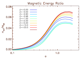
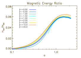
Figure 11: Values of the ratio $\mathcal{H}_{\rm tor}/\mathcal{H}$ for TT configurations with $\zeta=0$, in the presence of nonlinear terms in the definition of $\mathcal{M}$. Left panel: cases with $\nu=1$. Middle panel: cases with $\nu=4$. Right panel: cases with $\nu=10$.

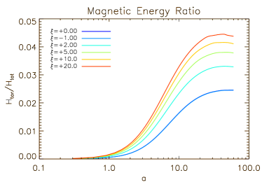
Figure 12: Values of the ratio $\mathcal{H}_{\rm tor}/\mathcal{H}$ for TR configurations with $\zeta=0$, in the presence of nonlinear terms in the definition of $\mathcal{M}$, with $\nu=4$.

4 Conclusion

In this work we investigated several equilibrium configurations for magnetized NSs, carrying out a detailed study of the parameter space. This allowed us to investigate general trends, and to sample the role of various current distributions. Interestingly we found that, almost insensitive of the chosen current distribution, the ratio $\mathcal{H}_{\rm tor}/\mathcal{H}$ never grows above 0.1.

We tried to use the same prescription for the current structure inside the star as the one used by CR13, but we, not only could not reproduce their results, but we got the opposite trend of a reduction in $\mathcal{H}_{\rm tor}/\mathcal{H}$, consistent with all the other results we have presented here. We pointed to a possible origin of this difference, related perhaps to the choice in the boundary conditions done by them, but because we are not able to impose such a boundary condition, further independent verification is needed to resolve this issue.

The failure to get toroidally dominated configurations, that are expected for stability in barotropic stars, might even point to the possibility that barotropicity does not hold in NS, and the entire stability problem is just related to entropy stratification (Reisenegger, 2009; Akgün et al., 2013), and not to the current distribution: a stably stratified NS can hold in place even a magnetic field out of MHD equilibrium.

On the other hand, the structure and strength of the magnetic field at the surface, is strongly influenced by the location and distribution of currents inside the star. We showed that magnetic field at the equator can in principle be much higher or much smaller than the value of the field at the pole. This means that the surface field can easily be dominated by higher multipoles than the dipole. It also implies that local processes, at or near the surface, might differ substantially, in their signatures, from the expectations of dipole dominated model, while on the other hand, processes related to the large scale field, as spin-down, will not. Interestingly, the result of the fully saturated non-linear regime, in the presence of subtractive currents, looks similar to what has recently been found in full time dependent MHD simulation of core collapse and Proto-NS formation in Supernovae by Obergaulinger, Janka & Aloy Toras (2014) (see the bottom panel of their Figure 14). The reason is due to the fact that turbulent eddies tend to expel magnetic field (Moffatt, 1978), which concentrates toward the axis, and becomes almost tangential at the proto-NS surface. Of course turbulence introduces also small scales, which however are likely to the first to be dissipated by any resistivity, leaving only the large scale structure at later times.

We also showed that mass and central rest mass density can affect the energetic properties of the magnetic field. In principle higher ratios of $\mathcal{H}_{\rm tor}/\mathcal{H}$ are reached for more massive and denser NSs. This might suggest that magnetars are NSs with higher mass than the average $1.4-1.5M_{\odot}$. It also stresses the importance and the role of the EoS, in determining possible electromagnetic properties and signatures of the NS.

Appendix A Antisymmetric Solutions

.

As we already discussed in Sect.3.1, the parity of the magnetic field, with respect to the equator, depends on the parity of the linear current term in the magnetization function $\mathcal{M}$. All the solutions that we have shown previously are symmetric (for $A_{\phi}$) with respect to the equator because this linear current term is proportional to the rest mass density. This is a requirement built into the integrability condition leading to the Bernoulli integral of Euler equation. It fixes the possible functional forms of $\mathcal{M}$. If one is willing to relax the global integrability condition, by allowing for example singular surface currents, it is possible to obtain antisymmetric solutions. Due to the presence of a surface current, there will be a jump in the parallel component of the magnetic field at the surface. However, introducing non linear current terms in $\mathcal{M}$, one can go to the fully non linear saturated regime, where the contribution of the linear current term becomes negligible, and make the residual jump in the magnetic field at the surface arbitrarily small. The non linear current term will preserve the parity of the surface current. We stress that, in this case, equilibrium and integrability hold inside the star, except at the surface itself.

If we choose for $\mathcal{M}$ the following functional form:

$$\mathcal{M}(A_{\phi})=k_{\rm pol}A_{\phi}\left[\frac{\xi}{\nu+1}\left(\frac{A_{\phi}}{A_{\phi}^{\rm max}}\right)^{\nu}\right],$$ (16)

and add to the current $J^{\phi}$ [see Eq. (8)], that enters the Grad-Shafranov Eq. (9), a singular current term:

$$k_{\rm pol}\cos{\theta}~{}\delta(r-R_{NS}),$$ (17)

by rising the value of $\xi$ one can find solutions that are independent of the strength of the surface current. We show in Fig. 13 the result in the case $\nu=1$, $\xi=50$. The jump at the surface is much smaller than the value of the magnetic field, and the solution can be assumed to be smooth. The result is dominated by the quadrupolar component.

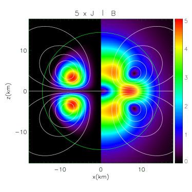
Figure 13: Antisymmetric solution, with $\nu=1$. Left panel: azimuthal current density normalized to 0.2 times its maximum. Right panel: magnetic field strength, normalized to the value at the pole. White contours represent magnetic field surfaces (isocontours of $A_{\phi}$). The thick green line is the stellar surface. Axes refer to a cartesian frame centered on the origin and with the $z$-axis corresponding to the symmetry axis.

Note that the symmetry of the current term only fixes the symmetry of the final solution. Every symmetric current will lead to the same symmetric field, which depends only on $\nu$, while every antisymmetric function will lead to the same antisymmetric field, which again depends on $\nu$ alone. With this approach it is not possible to produce for example octupolar models (where the dipole and quadrupole components are absent). Even the use of an octupolar surface current leads to dipolar configurations, in the fully saturated nonlinear regime. In the presence of non linear current term, multipoles are not eigenfunctions of the Grad Shafranov, and mode mixing is introduced. For the values of $\nu$ that we investigated, there is always a leading dipole component in the symmetric case, and a leading quadrupole component in the antisymmetric case, even if the strength of higher order multipoles at the surface can be relevant.

Appendix B Strong Field Regime

Our formalism allows us to extend the solutions computed in the weak field regime to the strong field regime to evaluate, for example, the related deformation induced by the magnetic field. In the strong field regime, however, the solution depends on the strength of the field. A detailed study of the induced deformation in the case of a purely poloidal field with $\xi=0$, and of TT configurations with $\zeta=0$, has already been presented by Pili, Bucciantini & Del Zanna (2014a). In that work there was also an investigation of the role of non linear current terms in $\mathcal{M}$, but only for $\nu=1$ and for small values of $\xi$ far from the fully non linear saturated regime. The present results, about TT configurations with various values of $\zeta$, show that $\mathcal{H}_{\rm tor}/\mathcal{H}$ have similar trends to the $\zeta=0$ case, and is always smaller than 0.1. We expect the deformation to be similar to what was found in Pili, Bucciantini & Del Zanna (2014a). On the other hand we have shown that, for purely poloidal fields, the non linear current term can substantially modify the field structure.

In Fig. 14 we plot the deformation rate $e$, and the relative variation of the circularization radius $\Delta R_{\rm circ}$, as defined by Pili, Bucciantini & Del Zanna (2014a), for purely poloidal configuration with various values of $\nu$, and with values of $\xi$ chosen such that the fully non linear regime is reached, both for subtractive and additive terms. Note that, for subtractive currents, the deformation rate is insensitive to the values of $\nu$, because, as we have shown, in the subtractive case, the resulting magnetic field is only very weakly dependent on $\nu$. On the other hand, substantial differences are observed in the case of additive currents.

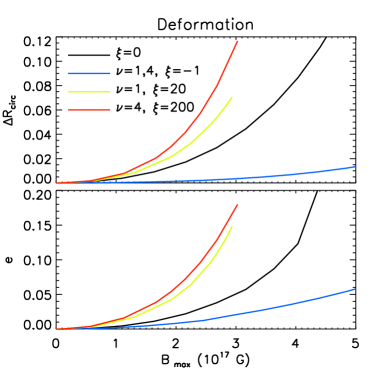
Figure 14: Upper panel: relative variation of the circularization radius as a function of the maximum strength of the magnetic field inside the star, for various values of $nu$ and $\xi$. Lower panel: deformation rate as a function of the maximum strength of the magnetic field inside the star. These sequences are done for a constant gravitational mass $M=1.4M_{\odot}$.

Subtractive currents tend to concentrate the field toward the center. This leads to significative changes of the rest mass density distribution limited to the core (structures with two rest mass density peaks can be reached) without affecting the rest of the star. As a consequence, the deformation rate, being related to the moment of inertia, changes less than in the case $\xi=0$, where a more uniformly distributed magnetic field affects also the outer layers. On the contrary, additive non linear currents tend to concentrate the field toward the edge of the star, and thus to produce a stronger deformation. This trend is evident in the circularization radius. This radius is almost unchanged for $\xi=-1$, while for $\xi>0$ the field causes a larger expansion of the outer layers of the star. Note that for $\xi=0,-1$ and for $\nu=1$ the maximum magnetic field strength is reached at the center. For $\nu=4$ and $\xi>>1$ it is reached half way trough the star (see Fig. 2).

References

- Akgün et al. (2013) Akgün T., Reisenegger A., Mastrano A., Marchant P., 2013, MNRAS, 433, 2445
- Armaza et al. (2014) Armaza C., Reisenegger A., Valdivia J. A., Marchant P., 2014, in IAU Symposium, Vol. 302, IAU Symposium, pp. 419–422
- Bocquet et al. (1995) Bocquet M., Bonazzola S., Gourgoulhon E., Novak J., 1995, A&A, 301, 757
- Bonanno, Rezzolla & Urpin (2003) Bonanno A., Rezzolla L., Urpin V., 2003, A&A, 410, L33
- Braithwaite (2009) Braithwaite J., 2009, MNRAS, 397, 763
- Braithwaite & Nordlund (2006) Braithwaite J., Nordlund Å., 2006, A&A, 450, 1077
- Braithwaite & Spruit (2006) Braithwaite J., Spruit H. C., 2006, A&A, 450, 1097
- Bucciantini & Del Zanna (2011) Bucciantini N., Del Zanna L., 2011, A&A, 528, A101
- Chamel & Haensel (2008) Chamel N., Haensel P., 2008, Living Reviews in Relativity, 11, 10
- Ciolfi, Ferrari & Gualtieri (2010) Ciolfi R., Ferrari V., Gualtieri L., 2010, MNRAS, 406, 2540
- Ciolfi et al. (2009) Ciolfi R., Ferrari V., Gualtieri L., Pons J. A., 2009, MNRAS, 397, 913
- Ciolfi & Rezzolla (2013) Ciolfi R., Rezzolla L., 2013, MNRAS
- Duncan & Thompson (1992) Duncan R. C., Thompson C., 1992, ApJLett, 392, L9
- Font (2008) Font J. A., 2008, Living Reviews in Relativity, 11, 7
- Frieben & Rezzolla (2012) Frieben J., Rezzolla L., 2012, MNRAS, 427, 3406
- Fujisawa, Yoshida & Eriguchi (2012) Fujisawa K., Yoshida S., Eriguchi Y., 2012, MNRAS, 422, 434
- Glampedakis, Andersson & Lander (2012) Glampedakis K., Andersson N., Lander S. K., 2012, MNRAS, 420, 1263
- Goldreich & Julian (1969) Goldreich P., Julian W. H., 1969, ApJ, 157, 869
- Haskell et al. (2008) Haskell B., Samuelsson L., Glampedakis K., Andersson N., 2008, MNRAS, 385, 531
- Ilgisonis & Pozdnyakov (2003) Ilgisonis V., Pozdnyakov Y., 2003, in APS Meeting Abstracts, p. 1107P
- Kiuchi, Kotake & Yoshida (2009) Kiuchi K., Kotake K., Yoshida S., 2009, ApJ, 698, 541
- Kiuchi & Yoshida (2008) Kiuchi K., Yoshida S., 2008, Phys. Rev. D, 78, 044045
- Konno (2001) Konno K., 2001, A&A, 372, 594
- Lander & Jones (2009) Lander S. K., Jones D. I., 2009, MNRAS, 395, 2162
- Lattimer (2012) Lattimer J. M., 2012, Annual Review of Nuclear and Particle Science, 62, 485
- Mereghetti (2008) Mereghetti S., 2008, A&A Rev., 15, 225
- Moffatt (1978) Moffatt H. K., 1978, Magnetic field generation in electrically conducting fluids
- Obergaulinger, Janka & Aloy Toras (2014) Obergaulinger M., Janka T., Aloy Toras M. A., 2014, ArXiv e-prints
- Pili, Bucciantini & Del Zanna (2014a) Pili A. G., Bucciantini N., Del Zanna L., 2014a, MNRAS, 439, 3541
- Pili, Bucciantini & Del Zanna (2014b) —, 2014b, International Journal of Modern Physics Conference Series, 28, 60202
- Pili, Bucciantini & Del Zanna (2014c) —, 2014c, ArXiv e-prints
- Pons et al. (1999) Pons J. A., Reddy S., Prakash M., Lattimer J. M., Miralles J. A., 1999, ApJ, 513, 780
- Reisenegger (2009) Reisenegger A., 2009, A&A, 499, 557
- Rheinhardt & Geppert (2005) Rheinhardt M., Geppert U., 2005, A&A, 435, 201
- Tchekhovskoy, Spitkovsky & Li (2013) Tchekhovskoy A., Spitkovsky A., Li J. G., 2013, MNRAS, 435, L1
- Thompson & Duncan (1993) Thompson C., Duncan R. C., 1993, ApJ, 408, 194
- Thompson, Burrows & Meyer (2001) Thompson T. A., Burrows A., Meyer B. S., 2001, ApJ, 562, 887
- Yakovlev et al. (2005) Yakovlev D. G., Gnedin O. Y., Gusakov M. E., Kaminker A. D., Levenfish K. P., Potekhin A. Y., 2005, Nuclear Physics A, 752, 590
- Yakovlev & Pethick (2004) Yakovlev D. G., Pethick C. J., 2004, ARA&A, 42, 169
- Yazadjiev (2012) Yazadjiev S. S., 2012, Phys. Rev. D, 85, 044030
- Yoshida, Yoshida & Eriguchi (2006) Yoshida S., Yoshida S., Eriguchi Y., 2006, ApJ, 651, 462