A sixth order averaged vector field method

Abstract

In this paper, based on the theory of rooted trees and B-series, we propose the concrete formulas of the substitution law for the trees of order $=5$. With the help of the new substitution law, we derive a B-series integrator extending the averaged vector field (AVF) method to high order. The new integrator turns out to be of order six and exactly preserves energy for Hamiltonian systems. Numerical experiments are presented to demonstrate the accuracy and the energy-preserving property of the sixth order AVF method.

Mathematics Subject Classfication  65D17 $\cdot$ 65L05 $\cdot$ 65P10

1 Introduction

Geometric numerical integration methods have come to the fore, partly as an alternative to traditional methods such as Runge-Kutta methods. A numerical method is called geometric if it preserves one or more physical/geometric properties of the system exactly (i.e. up to round-off error) Ref3 ; Ref1 ; Ref2 ; Ref4 . Examples of such geometric properties that can be preserved are (first) integrals, symplectic structures, symmetries and reversing symmetries, phase-space volumes, Lyapunov functions, foliations, etc. Geometric methods have applications in many areas of physics, including celestial mechanics, particle accelerators, molecular dynamics, fluid dynamics, pattern formation, plasma physics, reaction-diffusion equations, and meteorology Ref9 ; Ref5 ; Ref6 ; Ref10 ; RefQH ; Ref7 ; Ref8 ; RefW .

In fact, the conservation of the energy function is one of the most relevant features characterizing a Hamiltonian system. Methods that exactly preserve energy have been considered since several decades. Many energy-preserving methods have been proposed Ref14 ; Ref11 ; Ref13 ; Ref15 ; Ref12 . The discrete gradient method is among the most popular methods for designing integral preserving schemes for ordinary differential equations, which was perhaps first discussed by O. Gonzalez Ref16 . T. Matsuo proposed discrete variational method for nonlinear wave equation Ref17 . L. Brugnano and F. Iavernaro proposed Hamiltonian boundary value methods Ref18 ; Ref19 . More recently, the existence of energy-preserving B-series methods has been shown in Ref20 , and a practical integrator which is the averaged vector field (AVF) method of order two has been proposed Ref14 ; Ref11 ; Ref21 ; Ref22 . This method exactly preserves the energy of Hamiltonian systems, and in contrast to projection-type integrators, only requires evaluations of the vector field. It is symmetric and its Taylor series has the structure of a B-series. For polynomial Hamiltonians, the integral can be evaluated exactly, and the implementation is comparable to that of the implicit mid-point rule Ref12 .

In recent years, there has been growing interest in high-order AVF methods, and the second, third and fourth order AVF methods have been proposed Ref22 . It is shown that the theory of B-series and the substitution law obtained by substituting a B-series into the vector field appearing in another B-series play an important role in constructing high order methods Ref20 ; Ref5 . The substitution law for the trees of order $\leq 4$ has been shown in Ref23 ; Ref24 ; Ref5 . The fourth order AVF method is obtained by the concrete formulas of the substitution law for the trees of order $\leq 4$. To construct a B-series method which not only has high order accuracy but also preserves the Hamiltonian is an important and interesting topic. However, the concrete formulas of the substitution law for the trees of order $\geq 5$ have not been proposed, as the corresponding calculations are sufficiently complicated.

There are two aims in this paper. The first aim is to propose the concrete formulas of the substitution law for the trees of order $=5$. As we know, a low order B-series integrator can be extend to high order by the substitution law. Using the new obtained concrete formulas of the substitution law for the trees of order $=5$, one can extend a low order geometric B-series integrator to sixth order naturally, easily and automatically, such as the symplectic integrator, the energy-preserving integrator, the momentum-preserving integrator and so on. Using the new obtained substitution law, we also easily obtained the same sixth order symplectic integrator in Ref24 . The second aim is to derive a sixth order AVF method for Hamiltonian systems. By expanding the second order AVF method into a B-series and considering the substitution law for the trees of order $=5$, a new method can be constructed. The new method is derived by the concrete formulas of the substitution law for the trees of order $=5$. We prove that the new method is of order six and can also preserve the energy of Hamiltonian systems exactly.

The paper is organized as follows: In Sect. 2, we introduce the AVF method. In Sect. 3, we recall a few definitions and properties related to trees and B-series. The substitution law for the trees of order $\leq 4$ is shown and we obtain that for the trees of order $=5$. In Sect. 4, we derive the sixth order AVF method, and prove that the new method is of order six and it can preserve the Hamiltonian. A few numerical experiments are given in Sect. 5 to confirm the theoretical results. We finish the paper with conclusions in Sect. 6.

2 The AVF method and its energy conservation property

Here we briefly discuss the AVF method and its energy-conservation property. We consider a Hamiltonian differential equation, written in the form

$$\dot{z}=f(z)=S\nabla H(z),\quad z(0)=z_{0},\quad z\in\mathbb{R}^{n},$$ (1)

where $f(z):\mathbb{R}^{n}\rightarrow\mathbb{R}$, $S$ is a skew-symmetric constant matrix, $n$ is an even number, and the Hamiltonian $H(z)$ is assumed to be sufficiently differentiable. From system (1), we can get

$$\frac{dH(z(t))}{dt}=\nabla H(z)^{T}f(z)=\nabla H(z)^{T}S\nabla H(z)=0.$$ (2)

Therefore, the flow of the system (1) preserves the Hamiltonian $H(z)$ exactly.

The so-called AVF method Ref14 ; Ref22 is defined by

$$\frac{z_{1}-z_{0}}{h}=\int_{0}^{1}f(\xi z_{1}+(1-\xi)z_{0})d\xi,$$ (3)

where $h$ is the time step.

The AVF method (3) can be rewritten as

$$\frac{z_{1}-z_{0}}{h}=S\int_{0}^{1}\nabla H(\xi z_{1}+(1-\xi)z_{0})d\xi.$$

We can obtain

$$\frac{1}{h}(H(z_{1})-H(z_{0}))=\frac{1}{h}\int_{0}^{1}\frac{d}{d\xi}H(\xi z_{1}+(1-\xi)z_{0})d\xi$$

$$= (\int_{0}^{1}\nabla H(\xi z_{1}+(1-\xi)z_{0})d\xi)^{T}(\frac{z_{1}-z_{0}}{h})$$

$$= (\int_{0}^{1}\nabla H(\xi z_{1}+(1-\xi)z_{0})d\xi)^{T}S\int_{0}^{1}\nabla H(\xi z_{1}+(1-\xi)z_{0})d\xi=0.$$

It follows that the Hamiltonian $H$ is conserved at every time step.

R. I. McLachlan and G. R. W. Quispel also proposed a higher order energy-preserving method Ref22

$$\frac{z_{1}^{i}-z_{0}^{i}}{h}=(\delta_{j}^{i}+\alpha h^{2}f_{k}^{i}(\hat{z})f_{j}^{k}(\hat{z}))\int_{0}^{1}f^{j}(\xi z_{1}+(1-\xi)z_{0})d\xi,$$ (4)

where $\alpha$ is an arbitrary constant, $\delta_{i}^{j}$ is the Kronecker delta, and we can take e.g. $\hat{z}=z_{0}$ or $\hat{z}=\frac{z_{0}+z_{1}}{2}$. For $\alpha=0$, we recover the second order method (3). For $\alpha=-\frac{1}{12}$ and $\hat{z}=z_{0}$, the method is of order three. For $\alpha=-\frac{1}{12}$ and $\hat{z}=\frac{z_{0}+z_{1}}{2}$, the method is of order four.

The highest order of existing AVF method is four, and based on the theory of substitution law we can obtain a new AVF method of order six.

3 Preliminaries

In this section, we briefly recall a few definitions and properties related to rooted trees and B-series Ref25 ; Ref23 ; Ref24 ; Ref27 ; Ref20 ; Ref5 ; Ref6 ; Ref2 ; Ref26 .

3.1 Trees and B-series

Let $\emptyset$ denote the empty tree.

Definition 1 (Unordered trees Ref5 )

The set $\mathcal{T}$ of (rooted) unordered trees is recursively defined by

$$\begin{picture}(7.0,6.0)(0.0,0.0)\allinethickness{0.65pt} \put(3.5,2.5){\circle*{2.0}} \end{picture}\in\mathcal{T},\quad[\tau_{1},\ldots,\tau_{m}]\in\mathcal{T},\quad\forall~{}\tau_{1},\ldots,\tau_{m}\in\mathcal{T},$$ (5)

where is the tree with only one vertex, and $\tau=[\tau_{1},\ldots,\tau_{m}]$ represents the rooted tree obtained by grafting the roots of $\tau_{1},\ldots,\tau_{m}\in\mathcal{T}$ to a new vertex. Trees $\tau_{i}$ are called the branches of $\tau$.

We note that $\tau$ does not depend on the ordering of $\tau_{1},\ldots,\tau_{m}$. For instance, we do not distinguish between $[\begin{picture}(7.0,6.0)(0.0,0.0)\allinethickness{0.65pt} \put(3.5,2.5){\circle*{2.0}} \end{picture},[\begin{picture}(7.0,6.0)(0.0,0.0)\allinethickness{0.65pt} \put(3.5,2.5){\circle*{2.0}} \end{picture}]]$ and $[[\begin{picture}(7.0,6.0)(0.0,0.0)\allinethickness{0.65pt} \put(3.5,2.5){\circle*{2.0}} \end{picture}],\begin{picture}(7.0,6.0)(0.0,0.0)\allinethickness{0.65pt} \put(3.5,2.5){\circle*{2.0}} \end{picture}]$.

Definition 2 (Coefficients Ref2 )

The following coefficients are defined recursively for all trees $\tau=[\tau_{1},\ldots,\tau_{m}]\in\mathcal{T}$:

$$|\tau|~{}=~{} 1+\sum_{i=1}^{m}|\tau_{i}|\quad (the~{}order,~{}i.e.~{}the~{}number~{}of~{}vertices),$$

$$\alpha(\tau)~{}=~{} \frac{(|\tau|-1)!}{|\tau_{1}|!\cdot\ldots\cdot|\tau_{m}|!}\alpha(\tau_{1})\cdot\ldots\cdot\alpha(\tau_{m})\frac{1}{\mu_{1}!\mu_{2}!\ldots}\quad (Connes-Moscovici~{}weights),$$

$$\sigma(\tau)~{}=~{} \alpha(\tau_{1})\cdot\ldots\cdot\alpha(\tau_{m})\cdot\mu_{1}!\mu_{2}!\cdot\ldots\quad (symmetry),$$

$$\gamma(\tau)~{}=~{} |\tau|\gamma(\tau_{1})\cdot\ldots\cdot\gamma(\tau_{m})\quad (density),$$

where the integers $\mu_{1},\mu_{2},\ldots$ count equal trees among $\tau_{1},\ldots,\tau_{m}$.

Definition 3 (Elementary differentials Ref23 )

For a vector field $f:\mathbb{R}^{d}\rightarrow\mathbb{R}^{d}$, and for an unordered tree $\tau=[\tau_{1},\ldots,\tau_{m}]\in\mathcal{T}$, the so-called elementary differential is a mapping $F_{f}(\tau):\mathbb{R}^{d}\rightarrow\mathbb{R}^{d}$, recursively defined by

$$F_{f}(\begin{picture}(7.0,6.0)(0.0,0.0)\allinethickness{0.65pt} \put(3.5,2.5){\circle*{2.0}} \end{picture})(z)=f(z),\quad F_{f}(\tau)(z)=f^{m}(z)(F_{f}(\tau_{1})(z),\ldots,F_{f}(\tau_{m})(z)).$$

Definition 4 (B-series Ref26 )

For a mapping $a:\mathcal{T}\bigcup\{\emptyset\}\rightarrow\mathbb{R}$, a formal series of the form

$$B_{f}(a,z)=a(\emptyset)z+\sum_{\tau\in\mathcal{T}}\frac{h^{|\tau|}}{\sigma(\tau)}a(\tau)F_{f}(\tau)(z)$$

is called a B-series.

Theorem 3.1 (Exact solution Ref2 )

If $z(t)$ denotes the exact solution of (1), it holds for all $j\geq 1$,

$$\frac{1}{j!}z^{(j)}(0)=\sum_{\tau\in\mathcal{T},|\tau|=j}\frac{1}{\sigma(\tau)\gamma(\tau)}F_{f}(\tau)(z_{0}).$$

Therefore, letting $\gamma(\emptyset)=1$, the exact solution of (1) is (formally) given by

$$z(h)=B_{f}(\frac{1}{\gamma},z_{0}).$$

3.2 Basic tools for trees

3.2.1 Partitions and skeletons

In order to manipulate trees more conveniently, it is useful to consider the set $\mathcal{OT}$ of ordered trees defined below.

Definition 5 (Ordered trees Ref2 )

The set $\mathcal{OT}$ of ordered trees is recursively defined by

$$\begin{picture}(7.0,6.0)(0.0,0.0)\allinethickness{0.65pt} \put(3.5,2.5){\circle*{2.0}} \end{picture}\in\mathcal{OT},\quad(\omega_{1},\ldots,\omega_{m})\in\mathcal{OT},\quad\forall~{}\omega_{1},\ldots,\omega_{m}\in\mathcal{OT}.$$

In contrast to $\mathcal{T}$, the ordered tree $\omega$ depends on the ordering $\omega_{1},\ldots,\omega_{m}$.

Neglecting the ordering, a tree $\tau\in\mathcal{T}$ can be considered as an equivalent class of ordered trees, denoted $\tau=\overline{\omega}$. Therefore, any function $\psi$ defined on $\mathcal{T}$ (such as order, symmetry, density,…) can be extended to $\mathcal{OT}$ by putting $\psi(\omega)=\psi(\overline{\omega})$ for all $\omega\in\mathcal{OT}$. Moreover, for all $\tau\in\mathcal{T}$, we can choose a tree $\omega(\tau)\in\mathcal{OT}$ such as $\tau=\overline{\omega(\tau)}$ Ref23 .

Definition 6 (Partitions of a tree Ref23 )

A partition $p^{\theta}$ of an ordered tree $\theta\in\mathcal{OT}$ is the (ordered) tree obtained from $\theta$ by replacing some of its edges by dashed ones. We denote $P(p^{\theta})=\{s_{1},\ldots,s_{k}\}$ the list of subtrees $s_{i}\in\mathcal{T}$ obtained from $p^{\theta}$ by removing dashed edges and by neglecting the ordering of each subtree. We denote $\#(p^{\theta})=k$ the number of $s_{i}$’s. We observe that precisely one of the $s_{i}$’s contains the root of $\theta$. We denote this distinguished tree by $R(p^{\theta})\in\mathcal{T}$. We denote $P^{\ast}(p^{\theta})=P(p^{\theta})\backslash\{R(p^{\theta})\}$ the list of $s_{i}$’s that do not contain the root of $\theta$. Eventually, the set of all partitions $p^{\theta}$ of $\theta$ is denoted $\mathcal{P}(\theta)$. Finally, for $\tau\in\mathcal{T}$, we put $\mathcal{P}(\tau)=\mathcal{P}(\omega(\tau))$ where $\omega(\tau)\in\mathcal{OT}$ is given in definition 5.

We observe that any tree $\tau\in\mathcal{T}$ has exactly $2^{|\tau|-1}$ partitions $p^{\tau}\in\mathcal{P}(\tau)$, and that different partitions may lead to the same list of subtrees $P(p^{\tau})$.

Definition 7 (Skeleton of a partition Ref27 )

The skeleton $\chi(p^{\tau})\in\mathcal{T}$ of a partition $p^{\tau}\in\mathcal{P}(\tau)$ of a tree $\tau\in\mathcal{T}$ is the tree obtained by replacing in $p^{\tau}$ each tree of $P(p^{\tau})$ by a single vertex and then dashed edges by solid ones. We can notice that $|\chi(p^{\tau})|=\#(p^{\tau})$.

3.2.2 Substitution law

Theorem 3.2 (Substitution law Ref23 ; Ref24 ; Ref5 )

Let $a,b:\mathcal{T}\bigcup\{\emptyset\}\rightarrow\mathbb{R}$ be two mappings with $b(\emptyset)=0$. Given a field $f:\mathbb{R}^{d}\rightarrow\mathbb{R}^{d}$, consider the (h-dependent) field $g:\mathbb{R}^{d}\rightarrow\mathbb{R}^{d}$ defined by

$$hg(z)=B_{f}(b,z),$$

Then, there exists a mapping $b\star a:\mathcal{T}\bigcup\{\emptyset\}\rightarrow\mathbb{R}$ satisfying

$$B_{g}(a,z)=B_{f}(b\star a,z),$$

and $b\star a$ is defined by

$$b\star a(\emptyset)=a(\emptyset),\quad\forall\tau\in\mathcal{T},b\star a(\tau)=\sum_{p^{\tau}\in\mathcal{P}(\tau)}a(\chi(p^{\tau}))\prod_{\delta\in P(p^{\tau})}b(\delta).$$ (6)

in Ref23 ; Ref5 , the concrete formulas of the substitution law for the trees of order $\leq 4$ was proposed (see table 1). In this paper, we obtain the concrete formulas of the substitution law for the trees of order $=5$ (see table 2).

Table 1: The concrete formulas of the substitution law $\star$ defined in (6) for trees of order $\leq 4$

$$b\star a(\emptyset)=~{} a(\emptyset),$$

$$b\star a(\begin{picture}(7.0,6.0)(0.0,0.0)\allinethickness{0.65pt} \put(3.5,2.5){\circle*{2.0}} \end{picture})=~{} a(\begin{picture}(7.0,6.0)(0.0,0.0)\allinethickness{0.65pt} \put(3.5,2.5){\circle*{2.0}} \end{picture})b(\begin{picture}(7.0,6.0)(0.0,0.0)\allinethickness{0.65pt} \put(3.5,2.5){\circle*{2.0}} \end{picture}),$$

$$b\star a(\begin{picture}(9.0,7.0)(0.0,0.0)\allinethickness{0.65pt} \put(3.0,-1.5){\circle*{2.0}} \put(6.0,6.5){\circle*{2.0}} \put(3.0,-1.5){\line(3,8){3.0}} \end{picture})=~{} a(\begin{picture}(7.0,6.0)(0.0,0.0)\allinethickness{0.65pt} \put(3.5,2.5){\circle*{2.0}} \end{picture})b(\begin{picture}(9.0,7.0)(0.0,0.0)\allinethickness{0.65pt} \put(3.0,-1.5){\circle*{2.0}} \put(6.0,6.5){\circle*{2.0}} \put(3.0,-1.5){\line(3,8){3.0}} \end{picture})+a(\begin{picture}(9.0,7.0)(0.0,0.0)\allinethickness{0.65pt} \put(3.0,-1.5){\circle*{2.0}} \put(6.0,6.5){\circle*{2.0}} \put(3.0,-1.5){\line(3,8){3.0}} \end{picture})b(\begin{picture}(7.0,6.0)(0.0,0.0)\allinethickness{0.65pt} \put(3.5,2.5){\circle*{2.0}} \end{picture})^{2},$$

$$b\star a(\begin{picture}(11.5,7.0)(0.0,0.0)\allinethickness{0.65pt} \put(5.8,-1.5){\circle*{2.0}} \put(9.2,6.5){\circle*{2.0}} \put(2.4,6.5){\circle*{2.0}} \put(5.8,-1.5){\line(34,80){3.4}} \put(5.8,-1.5){\line(-34,80){3.4}} \end{picture})=~{} a(\begin{picture}(7.0,6.0)(0.0,0.0)\allinethickness{0.65pt} \put(3.5,2.5){\circle*{2.0}} \end{picture})b(\begin{picture}(11.5,7.0)(0.0,0.0)\allinethickness{0.65pt} \put(5.8,-1.5){\circle*{2.0}} \put(9.2,6.5){\circle*{2.0}} \put(2.4,6.5){\circle*{2.0}} \put(5.8,-1.5){\line(34,80){3.4}} \put(5.8,-1.5){\line(-34,80){3.4}} \end{picture})+2a(\begin{picture}(9.0,7.0)(0.0,0.0)\allinethickness{0.65pt} \put(3.0,-1.5){\circle*{2.0}} \put(6.0,6.5){\circle*{2.0}} \put(3.0,-1.5){\line(3,8){3.0}} \end{picture})b(\begin{picture}(7.0,6.0)(0.0,0.0)\allinethickness{0.65pt} \put(3.5,2.5){\circle*{2.0}} \end{picture})b(\begin{picture}(9.0,7.0)(0.0,0.0)\allinethickness{0.65pt} \put(3.0,-1.5){\circle*{2.0}} \put(6.0,6.5){\circle*{2.0}} \put(3.0,-1.5){\line(3,8){3.0}} \end{picture})+a(\begin{picture}(11.5,7.0)(0.0,0.0)\allinethickness{0.65pt} \put(5.8,-1.5){\circle*{2.0}} \put(9.2,6.5){\circle*{2.0}} \put(2.4,6.5){\circle*{2.0}} \put(5.8,-1.5){\line(34,80){3.4}} \put(5.8,-1.5){\line(-34,80){3.4}} \end{picture})b(\begin{picture}(7.0,6.0)(0.0,0.0)\allinethickness{0.65pt} \put(3.5,2.5){\circle*{2.0}} \end{picture})^{3},$$

$$b\star a(\begin{picture}(9.0,7.0)(0.0,0.0)\allinethickness{0.65pt} \put(3.0,-1.5){\circle*{2.0}} \put(6.0,6.5){\circle*{2.0}} \put(3.0,14.5){\circle*{2.0}} \put(3.0,-1.5){\line(3,8){3.0}} \put(6.0,6.5){\line(-3,8){3.0}} \end{picture})=~{} a(\begin{picture}(7.0,6.0)(0.0,0.0)\allinethickness{0.65pt} \put(3.5,2.5){\circle*{2.0}} \end{picture})b(\begin{picture}(9.0,7.0)(0.0,0.0)\allinethickness{0.65pt} \put(3.0,-1.5){\circle*{2.0}} \put(6.0,6.5){\circle*{2.0}} \put(3.0,14.5){\circle*{2.0}} \put(3.0,-1.5){\line(3,8){3.0}} \put(6.0,6.5){\line(-3,8){3.0}} \end{picture})+2a(\begin{picture}(9.0,7.0)(0.0,0.0)\allinethickness{0.65pt} \put(3.0,-1.5){\circle*{2.0}} \put(6.0,6.5){\circle*{2.0}} \put(3.0,-1.5){\line(3,8){3.0}} \end{picture})b(\begin{picture}(7.0,6.0)(0.0,0.0)\allinethickness{0.65pt} \put(3.5,2.5){\circle*{2.0}} \end{picture})b(\begin{picture}(9.0,7.0)(0.0,0.0)\allinethickness{0.65pt} \put(3.0,-1.5){\circle*{2.0}} \put(6.0,6.5){\circle*{2.0}} \put(3.0,-1.5){\line(3,8){3.0}} \end{picture})+a(\begin{picture}(9.0,7.0)(0.0,0.0)\allinethickness{0.65pt} \put(3.0,-1.5){\circle*{2.0}} \put(6.0,6.5){\circle*{2.0}} \put(3.0,14.5){\circle*{2.0}} \put(3.0,-1.5){\line(3,8){3.0}} \put(6.0,6.5){\line(-3,8){3.0}} \end{picture})b(\begin{picture}(7.0,6.0)(0.0,0.0)\allinethickness{0.65pt} \put(3.5,2.5){\circle*{2.0}} \end{picture})^{3},$$

$$b\star a(\begin{picture}(17.0,7.0)(-5.0,0.0)\allinethickness{0.65pt} \put(3.2,-1.5){\line(62,80){6.2}} \put(3.2,-1.5){\line(-62,80){6.2}} \put(3.2,-1.5){\line(0,1){8.0}} \put(3.2,-1.5){\circle*{2.0}} \put(9.4,6.5){\circle*{2.0}} \put(-3.0,6.5){\circle*{2.0}} \put(3.2,6.5){\circle*{2.0}} \end{picture})=~{} a(\begin{picture}(7.0,6.0)(0.0,0.0)\allinethickness{0.65pt} \put(3.5,2.5){\circle*{2.0}} \end{picture})b(\begin{picture}(17.0,7.0)(-5.0,0.0)\allinethickness{0.65pt} \put(3.2,-1.5){\line(62,80){6.2}} \put(3.2,-1.5){\line(-62,80){6.2}} \put(3.2,-1.5){\line(0,1){8.0}} \put(3.2,-1.5){\circle*{2.0}} \put(9.4,6.5){\circle*{2.0}} \put(-3.0,6.5){\circle*{2.0}} \put(3.2,6.5){\circle*{2.0}} \end{picture})+3a(\begin{picture}(9.0,7.0)(0.0,0.0)\allinethickness{0.65pt} \put(3.0,-1.5){\circle*{2.0}} \put(6.0,6.5){\circle*{2.0}} \put(3.0,-1.5){\line(3,8){3.0}} \end{picture})b(\begin{picture}(7.0,6.0)(0.0,0.0)\allinethickness{0.65pt} \put(3.5,2.5){\circle*{2.0}} \end{picture})b(\begin{picture}(11.5,7.0)(0.0,0.0)\allinethickness{0.65pt} \put(5.8,-1.5){\circle*{2.0}} \put(9.2,6.5){\circle*{2.0}} \put(2.4,6.5){\circle*{2.0}} \put(5.8,-1.5){\line(34,80){3.4}} \put(5.8,-1.5){\line(-34,80){3.4}} \end{picture})+3a(\begin{picture}(11.5,7.0)(0.0,0.0)\allinethickness{0.65pt} \put(5.8,-1.5){\circle*{2.0}} \put(9.2,6.5){\circle*{2.0}} \put(2.4,6.5){\circle*{2.0}} \put(5.8,-1.5){\line(34,80){3.4}} \put(5.8,-1.5){\line(-34,80){3.4}} \end{picture})b(\begin{picture}(7.0,6.0)(0.0,0.0)\allinethickness{0.65pt} \put(3.5,2.5){\circle*{2.0}} \end{picture})^{2}b(\begin{picture}(9.0,7.0)(0.0,0.0)\allinethickness{0.65pt} \put(3.0,-1.5){\circle*{2.0}} \put(6.0,6.5){\circle*{2.0}} \put(3.0,-1.5){\line(3,8){3.0}} \end{picture})+a(\begin{picture}(17.0,7.0)(-5.0,0.0)\allinethickness{0.65pt} \put(3.2,-1.5){\line(62,80){6.2}} \put(3.2,-1.5){\line(-62,80){6.2}} \put(3.2,-1.5){\line(0,1){8.0}} \put(3.2,-1.5){\circle*{2.0}} \put(9.4,6.5){\circle*{2.0}} \put(-3.0,6.5){\circle*{2.0}} \put(3.2,6.5){\circle*{2.0}} \end{picture})b(\begin{picture}(7.0,6.0)(0.0,0.0)\allinethickness{0.65pt} \put(3.5,2.5){\circle*{2.0}} \end{picture})^{4},$$

$$b\star a(\begin{picture}(12.0,7.0)(1.0,0.0)\allinethickness{0.65pt} \put(7.0,-1.5){\line(34,80){3.4}} \put(7.0,-1.5){\line(-34,80){3.4}} \put(10.4,6.5){\line(-34,80){3.4}} \put(7.0,-1.5){\circle*{2.0}} \put(10.4,6.5){\circle*{2.0}} \put(3.6,6.5){\circle*{2.0}} \put(7.0,14.5){\circle*{2.0}} \end{picture})=~{} a(\begin{picture}(7.0,6.0)(0.0,0.0)\allinethickness{0.65pt} \put(3.5,2.5){\circle*{2.0}} \end{picture})b(\begin{picture}(12.0,7.0)(1.0,0.0)\allinethickness{0.65pt} \put(7.0,-1.5){\line(34,80){3.4}} \put(7.0,-1.5){\line(-34,80){3.4}} \put(10.4,6.5){\line(-34,80){3.4}} \put(7.0,-1.5){\circle*{2.0}} \put(10.4,6.5){\circle*{2.0}} \put(3.6,6.5){\circle*{2.0}} \put(7.0,14.5){\circle*{2.0}} \end{picture})+a(\begin{picture}(9.0,7.0)(0.0,0.0)\allinethickness{0.65pt} \put(3.0,-1.5){\circle*{2.0}} \put(6.0,6.5){\circle*{2.0}} \put(3.0,-1.5){\line(3,8){3.0}} \end{picture})b(\begin{picture}(7.0,6.0)(0.0,0.0)\allinethickness{0.65pt} \put(3.5,2.5){\circle*{2.0}} \end{picture})b(\begin{picture}(9.0,7.0)(0.0,0.0)\allinethickness{0.65pt} \put(3.0,-1.5){\circle*{2.0}} \put(6.0,6.5){\circle*{2.0}} \put(3.0,14.5){\circle*{2.0}} \put(3.0,-1.5){\line(3,8){3.0}} \put(6.0,6.5){\line(-3,8){3.0}} \end{picture})+a(\begin{picture}(9.0,7.0)(0.0,0.0)\allinethickness{0.65pt} \put(3.0,-1.5){\circle*{2.0}} \put(6.0,6.5){\circle*{2.0}} \put(3.0,-1.5){\line(3,8){3.0}} \end{picture})b(\begin{picture}(9.0,7.0)(0.0,0.0)\allinethickness{0.65pt} \put(3.0,-1.5){\circle*{2.0}} \put(6.0,6.5){\circle*{2.0}} \put(3.0,-1.5){\line(3,8){3.0}} \end{picture})^{2}+a(\begin{picture}(9.0,7.0)(0.0,0.0)\allinethickness{0.65pt} \put(3.0,-1.5){\circle*{2.0}} \put(6.0,6.5){\circle*{2.0}} \put(3.0,-1.5){\line(3,8){3.0}} \end{picture})b(\begin{picture}(7.0,6.0)(0.0,0.0)\allinethickness{0.65pt} \put(3.5,2.5){\circle*{2.0}} \end{picture})b(\begin{picture}(11.5,7.0)(0.0,0.0)\allinethickness{0.65pt} \put(5.8,-1.5){\circle*{2.0}} \put(9.2,6.5){\circle*{2.0}} \put(2.4,6.5){\circle*{2.0}} \put(5.8,-1.5){\line(34,80){3.4}} \put(5.8,-1.5){\line(-34,80){3.4}} \end{picture})$$

$$+2a(\begin{picture}(11.5,7.0)(0.0,0.0)\allinethickness{0.65pt} \put(5.8,-1.5){\circle*{2.0}} \put(9.2,6.5){\circle*{2.0}} \put(2.4,6.5){\circle*{2.0}} \put(5.8,-1.5){\line(34,80){3.4}} \put(5.8,-1.5){\line(-34,80){3.4}} \end{picture})b(\begin{picture}(7.0,6.0)(0.0,0.0)\allinethickness{0.65pt} \put(3.5,2.5){\circle*{2.0}} \end{picture})^{2}b(\begin{picture}(9.0,7.0)(0.0,0.0)\allinethickness{0.65pt} \put(3.0,-1.5){\circle*{2.0}} \put(6.0,6.5){\circle*{2.0}} \put(3.0,-1.5){\line(3,8){3.0}} \end{picture})+a(\begin{picture}(9.0,7.0)(0.0,0.0)\allinethickness{0.65pt} \put(3.0,-1.5){\circle*{2.0}} \put(6.0,6.5){\circle*{2.0}} \put(3.0,14.5){\circle*{2.0}} \put(3.0,-1.5){\line(3,8){3.0}} \put(6.0,6.5){\line(-3,8){3.0}} \end{picture})b(\begin{picture}(7.0,6.0)(0.0,0.0)\allinethickness{0.65pt} \put(3.5,2.5){\circle*{2.0}} \end{picture}^{2})b(\begin{picture}(9.0,7.0)(0.0,0.0)\allinethickness{0.65pt} \put(3.0,-1.5){\circle*{2.0}} \put(6.0,6.5){\circle*{2.0}} \put(3.0,-1.5){\line(3,8){3.0}} \end{picture})+a(\begin{picture}(12.0,7.0)(1.0,0.0)\allinethickness{0.65pt} \put(7.0,-1.5){\line(34,80){3.4}} \put(7.0,-1.5){\line(-34,80){3.4}} \put(10.4,6.5){\line(-34,80){3.4}} \put(7.0,-1.5){\circle*{2.0}} \put(10.4,6.5){\circle*{2.0}} \put(3.6,6.5){\circle*{2.0}} \put(7.0,14.5){\circle*{2.0}} \end{picture})b(\begin{picture}(7.0,6.0)(0.0,0.0)\allinethickness{0.65pt} \put(3.5,2.5){\circle*{2.0}} \end{picture})^{4},$$

$$b\star a(\begin{picture}(12.0,7.0)(3.8,0.0)\allinethickness{0.65pt} \put(9.8,-1.5){\line(0,1){8.0}} \put(9.8,6.5){\line(34,80){3.4}} \put(9.8,6.5){\line(-34,80){3.4}} \put(9.8,-1.5){\circle*{2.0}} \put(9.8,6.5){\circle*{2.0}} \put(13.2,14.5){\circle*{2.0}} \put(6.4,14.5){\circle*{2.0}} \end{picture})=~{} a(\begin{picture}(7.0,6.0)(0.0,0.0)\allinethickness{0.65pt} \put(3.5,2.5){\circle*{2.0}} \end{picture})b(\begin{picture}(12.0,7.0)(3.8,0.0)\allinethickness{0.65pt} \put(9.8,-1.5){\line(0,1){8.0}} \put(9.8,6.5){\line(34,80){3.4}} \put(9.8,6.5){\line(-34,80){3.4}} \put(9.8,-1.5){\circle*{2.0}} \put(9.8,6.5){\circle*{2.0}} \put(13.2,14.5){\circle*{2.0}} \put(6.4,14.5){\circle*{2.0}} \end{picture})+a(\begin{picture}(9.0,7.0)(0.0,0.0)\allinethickness{0.65pt} \put(3.0,-1.5){\circle*{2.0}} \put(6.0,6.5){\circle*{2.0}} \put(3.0,-1.5){\line(3,8){3.0}} \end{picture})b(\begin{picture}(7.0,6.0)(0.0,0.0)\allinethickness{0.65pt} \put(3.5,2.5){\circle*{2.0}} \end{picture})b(\begin{picture}(11.5,7.0)(0.0,0.0)\allinethickness{0.65pt} \put(5.8,-1.5){\circle*{2.0}} \put(9.2,6.5){\circle*{2.0}} \put(2.4,6.5){\circle*{2.0}} \put(5.8,-1.5){\line(34,80){3.4}} \put(5.8,-1.5){\line(-34,80){3.4}} \end{picture})+2a(\begin{picture}(9.0,7.0)(0.0,0.0)\allinethickness{0.65pt} \put(3.0,-1.5){\circle*{2.0}} \put(6.0,6.5){\circle*{2.0}} \put(3.0,-1.5){\line(3,8){3.0}} \end{picture})b(\begin{picture}(7.0,6.0)(0.0,0.0)\allinethickness{0.65pt} \put(3.5,2.5){\circle*{2.0}} \end{picture})b(\begin{picture}(9.0,7.0)(0.0,0.0)\allinethickness{0.65pt} \put(3.0,-1.5){\circle*{2.0}} \put(6.0,6.5){\circle*{2.0}} \put(3.0,14.5){\circle*{2.0}} \put(3.0,-1.5){\line(3,8){3.0}} \put(6.0,6.5){\line(-3,8){3.0}} \end{picture})+a(\begin{picture}(11.5,7.0)(0.0,0.0)\allinethickness{0.65pt} \put(5.8,-1.5){\circle*{2.0}} \put(9.2,6.5){\circle*{2.0}} \put(2.4,6.5){\circle*{2.0}} \put(5.8,-1.5){\line(34,80){3.4}} \put(5.8,-1.5){\line(-34,80){3.4}} \end{picture})b(\begin{picture}(7.0,6.0)(0.0,0.0)\allinethickness{0.65pt} \put(3.5,2.5){\circle*{2.0}} \end{picture})^{2}b(\begin{picture}(9.0,7.0)(0.0,0.0)\allinethickness{0.65pt} \put(3.0,-1.5){\circle*{2.0}} \put(6.0,6.5){\circle*{2.0}} \put(3.0,-1.5){\line(3,8){3.0}} \end{picture})$$

$$+2a(\begin{picture}(9.0,7.0)(0.0,0.0)\allinethickness{0.65pt} \put(3.0,-1.5){\circle*{2.0}} \put(6.0,6.5){\circle*{2.0}} \put(3.0,14.5){\circle*{2.0}} \put(3.0,-1.5){\line(3,8){3.0}} \put(6.0,6.5){\line(-3,8){3.0}} \end{picture})b(\begin{picture}(7.0,6.0)(0.0,0.0)\allinethickness{0.65pt} \put(3.5,2.5){\circle*{2.0}} \end{picture})^{2}b(\begin{picture}(9.0,7.0)(0.0,0.0)\allinethickness{0.65pt} \put(3.0,-1.5){\circle*{2.0}} \put(6.0,6.5){\circle*{2.0}} \put(3.0,-1.5){\line(3,8){3.0}} \end{picture})+a(\begin{picture}(12.0,7.0)(3.8,0.0)\allinethickness{0.65pt} \put(9.8,-1.5){\line(0,1){8.0}} \put(9.8,6.5){\line(34,80){3.4}} \put(9.8,6.5){\line(-34,80){3.4}} \put(9.8,-1.5){\circle*{2.0}} \put(9.8,6.5){\circle*{2.0}} \put(13.2,14.5){\circle*{2.0}} \put(6.4,14.5){\circle*{2.0}} \end{picture})b(\begin{picture}(7.0,6.0)(0.0,0.0)\allinethickness{0.65pt} \put(3.5,2.5){\circle*{2.0}} \end{picture})^{4},$$

$$b\star a(\begin{picture}(9.0,7.0)(0.0,0.0)\allinethickness{0.65pt} \put(3.0,-1.5){\line(34,80){3.4}} \put(6.0,6.5){\line(-34,80){3.4}} \put(3.0,14.5){\line(34,80){3.4}} \put(3.0,-1.5){\circle*{2.0}} \put(6.0,6.5){\circle*{2.0}} \put(3.0,14.5){\circle*{2.0}} \put(6.0,22.5){\circle*{2.0}} \end{picture})=~{} a(\begin{picture}(7.0,6.0)(0.0,0.0)\allinethickness{0.65pt} \put(3.5,2.5){\circle*{2.0}} \end{picture})b(\begin{picture}(9.0,7.0)(0.0,0.0)\allinethickness{0.65pt} \put(3.0,-1.5){\line(34,80){3.4}} \put(6.0,6.5){\line(-34,80){3.4}} \put(3.0,14.5){\line(34,80){3.4}} \put(3.0,-1.5){\circle*{2.0}} \put(6.0,6.5){\circle*{2.0}} \put(3.0,14.5){\circle*{2.0}} \put(6.0,22.5){\circle*{2.0}} \end{picture})+2a(\begin{picture}(9.0,7.0)(0.0,0.0)\allinethickness{0.65pt} \put(3.0,-1.5){\circle*{2.0}} \put(6.0,6.5){\circle*{2.0}} \put(3.0,-1.5){\line(3,8){3.0}} \end{picture})b(\begin{picture}(7.0,6.0)(0.0,0.0)\allinethickness{0.65pt} \put(3.5,2.5){\circle*{2.0}} \end{picture})b(\begin{picture}(9.0,7.0)(0.0,0.0)\allinethickness{0.65pt} \put(3.0,-1.5){\circle*{2.0}} \put(6.0,6.5){\circle*{2.0}} \put(3.0,14.5){\circle*{2.0}} \put(3.0,-1.5){\line(3,8){3.0}} \put(6.0,6.5){\line(-3,8){3.0}} \end{picture})+a(\begin{picture}(9.0,7.0)(0.0,0.0)\allinethickness{0.65pt} \put(3.0,-1.5){\circle*{2.0}} \put(6.0,6.5){\circle*{2.0}} \put(3.0,-1.5){\line(3,8){3.0}} \end{picture})b(\begin{picture}(9.0,7.0)(0.0,0.0)\allinethickness{0.65pt} \put(3.0,-1.5){\circle*{2.0}} \put(6.0,6.5){\circle*{2.0}} \put(3.0,-1.5){\line(3,8){3.0}} \end{picture})^{2}+3a(\begin{picture}(9.0,7.0)(0.0,0.0)\allinethickness{0.65pt} \put(3.0,-1.5){\circle*{2.0}} \put(6.0,6.5){\circle*{2.0}} \put(3.0,14.5){\circle*{2.0}} \put(3.0,-1.5){\line(3,8){3.0}} \put(6.0,6.5){\line(-3,8){3.0}} \end{picture})b(\begin{picture}(7.0,6.0)(0.0,0.0)\allinethickness{0.65pt} \put(3.5,2.5){\circle*{2.0}} \end{picture})^{2}b(\begin{picture}(9.0,7.0)(0.0,0.0)\allinethickness{0.65pt} \put(3.0,-1.5){\circle*{2.0}} \put(6.0,6.5){\circle*{2.0}} \put(3.0,-1.5){\line(3,8){3.0}} \end{picture})$$

$$+a(\begin{picture}(9.0,7.0)(0.0,0.0)\allinethickness{0.65pt} \put(3.0,-1.5){\line(34,80){3.4}} \put(6.0,6.5){\line(-34,80){3.4}} \put(3.0,14.5){\line(34,80){3.4}} \put(3.0,-1.5){\circle*{2.0}} \put(6.0,6.5){\circle*{2.0}} \put(3.0,14.5){\circle*{2.0}} \put(6.0,22.5){\circle*{2.0}} \end{picture})b(\begin{picture}(7.0,6.0)(0.0,0.0)\allinethickness{0.65pt} \put(3.5,2.5){\circle*{2.0}} \end{picture})^{4}.$$

Table 2: The concrete formulas of the substitution law $\star$ defined in (6) for trees of order $=5$

$$b\star a(\begin{picture}(19.0,7.0)(0.0,0.0)\allinethickness{0.65pt} \put(9.5,-1.5){\line(-75,80){7.5}} \put(9.5,-1.5){\line(-25,80){2.5}} \put(9.5,-1.5){\line(25,80){2.5}} \put(9.5,-1.5){\line(75,80){7.5}} \put(9.5,-1.5){\circle*{2.0}} \put(2.0,6.5){\circle*{2.0}} \put(7.0,6.5){\circle*{2.0}} \put(12.0,6.5){\circle*{2.0}} \put(17.0,6.5){\circle*{2.0}} \end{picture})=~{} a(\begin{picture}(7.0,6.0)(0.0,0.0)\allinethickness{0.65pt} \put(3.5,2.5){\circle*{2.0}} \end{picture})b(\begin{picture}(19.0,7.0)(0.0,0.0)\allinethickness{0.65pt} \put(9.5,-1.5){\line(-75,80){7.5}} \put(9.5,-1.5){\line(-25,80){2.5}} \put(9.5,-1.5){\line(25,80){2.5}} \put(9.5,-1.5){\line(75,80){7.5}} \put(9.5,-1.5){\circle*{2.0}} \put(2.0,6.5){\circle*{2.0}} \put(7.0,6.5){\circle*{2.0}} \put(12.0,6.5){\circle*{2.0}} \put(17.0,6.5){\circle*{2.0}} \end{picture})+4a(\begin{picture}(9.0,7.0)(0.0,0.0)\allinethickness{0.65pt} \put(3.0,-1.5){\circle*{2.0}} \put(6.0,6.5){\circle*{2.0}} \put(3.0,-1.5){\line(3,8){3.0}} \end{picture})b(\begin{picture}(7.0,6.0)(0.0,0.0)\allinethickness{0.65pt} \put(3.5,2.5){\circle*{2.0}} \end{picture})b(\begin{picture}(17.0,7.0)(-5.0,0.0)\allinethickness{0.65pt} \put(3.2,-1.5){\line(62,80){6.2}} \put(3.2,-1.5){\line(-62,80){6.2}} \put(3.2,-1.5){\line(0,1){8.0}} \put(3.2,-1.5){\circle*{2.0}} \put(9.4,6.5){\circle*{2.0}} \put(-3.0,6.5){\circle*{2.0}} \put(3.2,6.5){\circle*{2.0}} \end{picture})+6a(\begin{picture}(11.5,7.0)(0.0,0.0)\allinethickness{0.65pt} \put(5.8,-1.5){\circle*{2.0}} \put(9.2,6.5){\circle*{2.0}} \put(2.4,6.5){\circle*{2.0}} \put(5.8,-1.5){\line(34,80){3.4}} \put(5.8,-1.5){\line(-34,80){3.4}} \end{picture})b(\begin{picture}(7.0,6.0)(0.0,0.0)\allinethickness{0.65pt} \put(3.5,2.5){\circle*{2.0}} \end{picture})^{2}b(\begin{picture}(11.5,7.0)(0.0,0.0)\allinethickness{0.65pt} \put(5.8,-1.5){\circle*{2.0}} \put(9.2,6.5){\circle*{2.0}} \put(2.4,6.5){\circle*{2.0}} \put(5.8,-1.5){\line(34,80){3.4}} \put(5.8,-1.5){\line(-34,80){3.4}} \end{picture})$$

$$+4a(\begin{picture}(17.0,7.0)(-5.0,0.0)\allinethickness{0.65pt} \put(3.2,-1.5){\line(62,80){6.2}} \put(3.2,-1.5){\line(-62,80){6.2}} \put(3.2,-1.5){\line(0,1){8.0}} \put(3.2,-1.5){\circle*{2.0}} \put(9.4,6.5){\circle*{2.0}} \put(-3.0,6.5){\circle*{2.0}} \put(3.2,6.5){\circle*{2.0}} \end{picture})b(\begin{picture}(7.0,6.0)(0.0,0.0)\allinethickness{0.65pt} \put(3.5,2.5){\circle*{2.0}} \end{picture})^{3}b(\begin{picture}(9.0,7.0)(0.0,0.0)\allinethickness{0.65pt} \put(3.0,-1.5){\circle*{2.0}} \put(6.0,6.5){\circle*{2.0}} \put(3.0,-1.5){\line(3,8){3.0}} \end{picture})+a(\begin{picture}(19.0,7.0)(0.0,0.0)\allinethickness{0.65pt} \put(9.5,-1.5){\line(-75,80){7.5}} \put(9.5,-1.5){\line(-25,80){2.5}} \put(9.5,-1.5){\line(25,80){2.5}} \put(9.5,-1.5){\line(75,80){7.5}} \put(9.5,-1.5){\circle*{2.0}} \put(2.0,6.5){\circle*{2.0}} \put(7.0,6.5){\circle*{2.0}} \put(12.0,6.5){\circle*{2.0}} \put(17.0,6.5){\circle*{2.0}} \end{picture})b(\begin{picture}(7.0,6.0)(0.0,0.0)\allinethickness{0.65pt} \put(3.5,2.5){\circle*{2.0}} \end{picture})^{5},$$

$$b\star a(\begin{picture}(16.4,7.0)(0.0,0.0)\allinethickness{0.65pt} \put(8.2,-1.5){\line(62,80){6.2}} \put(8.2,-1.5){\line(-62,80){6.2}} \put(8.2,-1.5){\line(0,1){8.0}} \put(2.0,6.5){\line(62,80){6.2}} \put(8.2,-1.5){\circle*{2.0}} \put(14.4,6.5){\circle*{2.0}} \put(2.0,6.5){\circle*{2.0}} \put(8.2,6.5){\circle*{2.0}} \put(8.2,14.5){\circle*{2.0}} \end{picture})=~{} a(\begin{picture}(7.0,6.0)(0.0,0.0)\allinethickness{0.65pt} \put(3.5,2.5){\circle*{2.0}} \end{picture})b(\begin{picture}(16.4,7.0)(0.0,0.0)\allinethickness{0.65pt} \put(8.2,-1.5){\line(62,80){6.2}} \put(8.2,-1.5){\line(-62,80){6.2}} \put(8.2,-1.5){\line(0,1){8.0}} \put(2.0,6.5){\line(62,80){6.2}} \put(8.2,-1.5){\circle*{2.0}} \put(14.4,6.5){\circle*{2.0}} \put(2.0,6.5){\circle*{2.0}} \put(8.2,6.5){\circle*{2.0}} \put(8.2,14.5){\circle*{2.0}} \end{picture})+a(\begin{picture}(9.0,7.0)(0.0,0.0)\allinethickness{0.65pt} \put(3.0,-1.5){\circle*{2.0}} \put(6.0,6.5){\circle*{2.0}} \put(3.0,-1.5){\line(3,8){3.0}} \end{picture})b(\begin{picture}(7.0,6.0)(0.0,0.0)\allinethickness{0.65pt} \put(3.5,2.5){\circle*{2.0}} \end{picture})b(\begin{picture}(17.0,7.0)(-5.0,0.0)\allinethickness{0.65pt} \put(3.2,-1.5){\line(62,80){6.2}} \put(3.2,-1.5){\line(-62,80){6.2}} \put(3.2,-1.5){\line(0,1){8.0}} \put(3.2,-1.5){\circle*{2.0}} \put(9.4,6.5){\circle*{2.0}} \put(-3.0,6.5){\circle*{2.0}} \put(3.2,6.5){\circle*{2.0}} \end{picture})+2a(\begin{picture}(9.0,7.0)(0.0,0.0)\allinethickness{0.65pt} \put(3.0,-1.5){\circle*{2.0}} \put(6.0,6.5){\circle*{2.0}} \put(3.0,-1.5){\line(3,8){3.0}} \end{picture})b(\begin{picture}(7.0,6.0)(0.0,0.0)\allinethickness{0.65pt} \put(3.5,2.5){\circle*{2.0}} \end{picture})b(\begin{picture}(12.0,7.0)(1.0,0.0)\allinethickness{0.65pt} \put(7.0,-1.5){\line(34,80){3.4}} \put(7.0,-1.5){\line(-34,80){3.4}} \put(10.4,6.5){\line(-34,80){3.4}} \put(7.0,-1.5){\circle*{2.0}} \put(10.4,6.5){\circle*{2.0}} \put(3.6,6.5){\circle*{2.0}} \put(7.0,14.5){\circle*{2.0}} \end{picture})+a(\begin{picture}(9.0,7.0)(0.0,0.0)\allinethickness{0.65pt} \put(3.0,-1.5){\circle*{2.0}} \put(6.0,6.5){\circle*{2.0}} \put(3.0,-1.5){\line(3,8){3.0}} \end{picture})b(\begin{picture}(9.0,7.0)(0.0,0.0)\allinethickness{0.65pt} \put(3.0,-1.5){\circle*{2.0}} \put(6.0,6.5){\circle*{2.0}} \put(3.0,-1.5){\line(3,8){3.0}} \end{picture})b(\begin{picture}(11.5,7.0)(0.0,0.0)\allinethickness{0.65pt} \put(5.8,-1.5){\circle*{2.0}} \put(9.2,6.5){\circle*{2.0}} \put(2.4,6.5){\circle*{2.0}} \put(5.8,-1.5){\line(34,80){3.4}} \put(5.8,-1.5){\line(-34,80){3.4}} \end{picture})$$

$$+a(\begin{picture}(9.0,7.0)(0.0,0.0)\allinethickness{0.65pt} \put(3.0,-1.5){\circle*{2.0}} \put(6.0,6.5){\circle*{2.0}} \put(3.0,14.5){\circle*{2.0}} \put(3.0,-1.5){\line(3,8){3.0}} \put(6.0,6.5){\line(-3,8){3.0}} \end{picture})b(\begin{picture}(7.0,6.0)(0.0,0.0)\allinethickness{0.65pt} \put(3.5,2.5){\circle*{2.0}} \end{picture})^{2}b(\begin{picture}(11.5,7.0)(0.0,0.0)\allinethickness{0.65pt} \put(5.8,-1.5){\circle*{2.0}} \put(9.2,6.5){\circle*{2.0}} \put(2.4,6.5){\circle*{2.0}} \put(5.8,-1.5){\line(34,80){3.4}} \put(5.8,-1.5){\line(-34,80){3.4}} \end{picture})+2a(\begin{picture}(11.5,7.0)(0.0,0.0)\allinethickness{0.65pt} \put(5.8,-1.5){\circle*{2.0}} \put(9.2,6.5){\circle*{2.0}} \put(2.4,6.5){\circle*{2.0}} \put(5.8,-1.5){\line(34,80){3.4}} \put(5.8,-1.5){\line(-34,80){3.4}} \end{picture})b(\begin{picture}(7.0,6.0)(0.0,0.0)\allinethickness{0.65pt} \put(3.5,2.5){\circle*{2.0}} \end{picture})^{2}b(\begin{picture}(11.5,7.0)(0.0,0.0)\allinethickness{0.65pt} \put(5.8,-1.5){\circle*{2.0}} \put(9.2,6.5){\circle*{2.0}} \put(2.4,6.5){\circle*{2.0}} \put(5.8,-1.5){\line(34,80){3.4}} \put(5.8,-1.5){\line(-34,80){3.4}} \end{picture})+a(\begin{picture}(11.5,7.0)(0.0,0.0)\allinethickness{0.65pt} \put(5.8,-1.5){\circle*{2.0}} \put(9.2,6.5){\circle*{2.0}} \put(2.4,6.5){\circle*{2.0}} \put(5.8,-1.5){\line(34,80){3.4}} \put(5.8,-1.5){\line(-34,80){3.4}} \end{picture})b(\begin{picture}(7.0,6.0)(0.0,0.0)\allinethickness{0.65pt} \put(3.5,2.5){\circle*{2.0}} \end{picture})^{2}b(\begin{picture}(9.0,7.0)(0.0,0.0)\allinethickness{0.65pt} \put(3.0,-1.5){\circle*{2.0}} \put(6.0,6.5){\circle*{2.0}} \put(3.0,14.5){\circle*{2.0}} \put(3.0,-1.5){\line(3,8){3.0}} \put(6.0,6.5){\line(-3,8){3.0}} \end{picture})$$

$$+2a(\begin{picture}(11.5,7.0)(0.0,0.0)\allinethickness{0.65pt} \put(5.8,-1.5){\circle*{2.0}} \put(9.2,6.5){\circle*{2.0}} \put(2.4,6.5){\circle*{2.0}} \put(5.8,-1.5){\line(34,80){3.4}} \put(5.8,-1.5){\line(-34,80){3.4}} \end{picture})b(\begin{picture}(7.0,6.0)(0.0,0.0)\allinethickness{0.65pt} \put(3.5,2.5){\circle*{2.0}} \end{picture})b(\begin{picture}(9.0,7.0)(0.0,0.0)\allinethickness{0.65pt} \put(3.0,-1.5){\circle*{2.0}} \put(6.0,6.5){\circle*{2.0}} \put(3.0,-1.5){\line(3,8){3.0}} \end{picture})^{2}+2a(\begin{picture}(17.0,7.0)(-5.0,0.0)\allinethickness{0.65pt} \put(3.2,-1.5){\line(62,80){6.2}} \put(3.2,-1.5){\line(-62,80){6.2}} \put(3.2,-1.5){\line(0,1){8.0}} \put(3.2,-1.5){\circle*{2.0}} \put(9.4,6.5){\circle*{2.0}} \put(-3.0,6.5){\circle*{2.0}} \put(3.2,6.5){\circle*{2.0}} \end{picture})b(\begin{picture}(7.0,6.0)(0.0,0.0)\allinethickness{0.65pt} \put(3.5,2.5){\circle*{2.0}} \end{picture})^{3}b(\begin{picture}(9.0,7.0)(0.0,0.0)\allinethickness{0.65pt} \put(3.0,-1.5){\circle*{2.0}} \put(6.0,6.5){\circle*{2.0}} \put(3.0,-1.5){\line(3,8){3.0}} \end{picture})+2a(\begin{picture}(12.0,7.0)(1.0,0.0)\allinethickness{0.65pt} \put(7.0,-1.5){\line(34,80){3.4}} \put(7.0,-1.5){\line(-34,80){3.4}} \put(10.4,6.5){\line(-34,80){3.4}} \put(7.0,-1.5){\circle*{2.0}} \put(10.4,6.5){\circle*{2.0}} \put(3.6,6.5){\circle*{2.0}} \put(7.0,14.5){\circle*{2.0}} \end{picture})b(\begin{picture}(7.0,6.0)(0.0,0.0)\allinethickness{0.65pt} \put(3.5,2.5){\circle*{2.0}} \end{picture})^{3}b(\begin{picture}(9.0,7.0)(0.0,0.0)\allinethickness{0.65pt} \put(3.0,-1.5){\circle*{2.0}} \put(6.0,6.5){\circle*{2.0}} \put(3.0,-1.5){\line(3,8){3.0}} \end{picture})$$

$$+a(\begin{picture}(16.4,7.0)(0.0,0.0)\allinethickness{0.65pt} \put(8.2,-1.5){\line(62,80){6.2}} \put(8.2,-1.5){\line(-62,80){6.2}} \put(8.2,-1.5){\line(0,1){8.0}} \put(2.0,6.5){\line(62,80){6.2}} \put(8.2,-1.5){\circle*{2.0}} \put(14.4,6.5){\circle*{2.0}} \put(2.0,6.5){\circle*{2.0}} \put(8.2,6.5){\circle*{2.0}} \put(8.2,14.5){\circle*{2.0}} \end{picture})b(\begin{picture}(7.0,6.0)(0.0,0.0)\allinethickness{0.65pt} \put(3.5,2.5){\circle*{2.0}} \end{picture})^{5},$$

$$b\star a(\begin{picture}(16.4,7.0)(0.0,0.0)\allinethickness{0.65pt} \put(8.2,-1.5){\line(62,80){6.2}} \put(8.2,-1.5){\line(-62,80){6.2}} \put(14.4,6.5){\line(-30,80){3.0}} \put(2.0,6.5){\line(30,80){3.0}} \put(8.2,-1.5){\circle*{2.0}} \put(14.4,6.5){\circle*{2.0}} \put(2.0,6.5){\circle*{2.0}} \put(5.2,14.5){\circle*{2.0}} \put(11.2,14.5){\circle*{2.0}} \end{picture})=~{} a(\begin{picture}(7.0,6.0)(0.0,0.0)\allinethickness{0.65pt} \put(3.5,2.5){\circle*{2.0}} \end{picture})b(\begin{picture}(16.4,7.0)(0.0,0.0)\allinethickness{0.65pt} \put(8.2,-1.5){\line(62,80){6.2}} \put(8.2,-1.5){\line(-62,80){6.2}} \put(14.4,6.5){\line(-30,80){3.0}} \put(2.0,6.5){\line(30,80){3.0}} \put(8.2,-1.5){\circle*{2.0}} \put(14.4,6.5){\circle*{2.0}} \put(2.0,6.5){\circle*{2.0}} \put(5.2,14.5){\circle*{2.0}} \put(11.2,14.5){\circle*{2.0}} \end{picture})+2a(\begin{picture}(9.0,7.0)(0.0,0.0)\allinethickness{0.65pt} \put(3.0,-1.5){\circle*{2.0}} \put(6.0,6.5){\circle*{2.0}} \put(3.0,-1.5){\line(3,8){3.0}} \end{picture})b(\begin{picture}(7.0,6.0)(0.0,0.0)\allinethickness{0.65pt} \put(3.5,2.5){\circle*{2.0}} \end{picture})b(\begin{picture}(12.0,7.0)(1.0,0.0)\allinethickness{0.65pt} \put(7.0,-1.5){\line(34,80){3.4}} \put(7.0,-1.5){\line(-34,80){3.4}} \put(10.4,6.5){\line(-34,80){3.4}} \put(7.0,-1.5){\circle*{2.0}} \put(10.4,6.5){\circle*{2.0}} \put(3.6,6.5){\circle*{2.0}} \put(7.0,14.5){\circle*{2.0}} \end{picture})+2a(\begin{picture}(9.0,7.0)(0.0,0.0)\allinethickness{0.65pt} \put(3.0,-1.5){\circle*{2.0}} \put(6.0,6.5){\circle*{2.0}} \put(3.0,-1.5){\line(3,8){3.0}} \end{picture})b(\begin{picture}(9.0,7.0)(0.0,0.0)\allinethickness{0.65pt} \put(3.0,-1.5){\circle*{2.0}} \put(6.0,6.5){\circle*{2.0}} \put(3.0,-1.5){\line(3,8){3.0}} \end{picture})b(\begin{picture}(9.0,7.0)(0.0,0.0)\allinethickness{0.65pt} \put(3.0,-1.5){\circle*{2.0}} \put(6.0,6.5){\circle*{2.0}} \put(3.0,14.5){\circle*{2.0}} \put(3.0,-1.5){\line(3,8){3.0}} \put(6.0,6.5){\line(-3,8){3.0}} \end{picture})$$

$$+a(\begin{picture}(11.5,7.0)(0.0,0.0)\allinethickness{0.65pt} \put(5.8,-1.5){\circle*{2.0}} \put(9.2,6.5){\circle*{2.0}} \put(2.4,6.5){\circle*{2.0}} \put(5.8,-1.5){\line(34,80){3.4}} \put(5.8,-1.5){\line(-34,80){3.4}} \end{picture})b(\begin{picture}(7.0,6.0)(0.0,0.0)\allinethickness{0.65pt} \put(3.5,2.5){\circle*{2.0}} \end{picture})^{2}b(\begin{picture}(11.5,7.0)(0.0,0.0)\allinethickness{0.65pt} \put(5.8,-1.5){\circle*{2.0}} \put(9.2,6.5){\circle*{2.0}} \put(2.4,6.5){\circle*{2.0}} \put(5.8,-1.5){\line(34,80){3.4}} \put(5.8,-1.5){\line(-34,80){3.4}} \end{picture})+2a(\begin{picture}(9.0,7.0)(0.0,0.0)\allinethickness{0.65pt} \put(3.0,-1.5){\circle*{2.0}} \put(6.0,6.5){\circle*{2.0}} \put(3.0,14.5){\circle*{2.0}} \put(3.0,-1.5){\line(3,8){3.0}} \put(6.0,6.5){\line(-3,8){3.0}} \end{picture})b(\begin{picture}(7.0,6.0)(0.0,0.0)\allinethickness{0.65pt} \put(3.5,2.5){\circle*{2.0}} \end{picture})^{2}b(\begin{picture}(9.0,7.0)(0.0,0.0)\allinethickness{0.65pt} \put(3.0,-1.5){\circle*{2.0}} \put(6.0,6.5){\circle*{2.0}} \put(3.0,14.5){\circle*{2.0}} \put(3.0,-1.5){\line(3,8){3.0}} \put(6.0,6.5){\line(-3,8){3.0}} \end{picture})+3a(\begin{picture}(11.5,7.0)(0.0,0.0)\allinethickness{0.65pt} \put(5.8,-1.5){\circle*{2.0}} \put(9.2,6.5){\circle*{2.0}} \put(2.4,6.5){\circle*{2.0}} \put(5.8,-1.5){\line(34,80){3.4}} \put(5.8,-1.5){\line(-34,80){3.4}} \end{picture})b(\begin{picture}(7.0,6.0)(0.0,0.0)\allinethickness{0.65pt} \put(3.5,2.5){\circle*{2.0}} \end{picture})b(\begin{picture}(9.0,7.0)(0.0,0.0)\allinethickness{0.65pt} \put(3.0,-1.5){\circle*{2.0}} \put(6.0,6.5){\circle*{2.0}} \put(3.0,-1.5){\line(3,8){3.0}} \end{picture})^{2}$$

$$+4a(\begin{picture}(12.0,7.0)(1.0,0.0)\allinethickness{0.65pt} \put(7.0,-1.5){\line(34,80){3.4}} \put(7.0,-1.5){\line(-34,80){3.4}} \put(10.4,6.5){\line(-34,80){3.4}} \put(7.0,-1.5){\circle*{2.0}} \put(10.4,6.5){\circle*{2.0}} \put(3.6,6.5){\circle*{2.0}} \put(7.0,14.5){\circle*{2.0}} \end{picture})b(\begin{picture}(7.0,6.0)(0.0,0.0)\allinethickness{0.65pt} \put(3.5,2.5){\circle*{2.0}} \end{picture})^{3}b(\begin{picture}(9.0,7.0)(0.0,0.0)\allinethickness{0.65pt} \put(3.0,-1.5){\circle*{2.0}} \put(6.0,6.5){\circle*{2.0}} \put(3.0,-1.5){\line(3,8){3.0}} \end{picture})+a(\begin{picture}(16.4,7.0)(0.0,0.0)\allinethickness{0.65pt} \put(8.2,-1.5){\line(62,80){6.2}} \put(8.2,-1.5){\line(-62,80){6.2}} \put(14.4,6.5){\line(-30,80){3.0}} \put(2.0,6.5){\line(30,80){3.0}} \put(8.2,-1.5){\circle*{2.0}} \put(14.4,6.5){\circle*{2.0}} \put(2.0,6.5){\circle*{2.0}} \put(5.2,14.5){\circle*{2.0}} \put(11.2,14.5){\circle*{2.0}} \end{picture})b(\begin{picture}(7.0,6.0)(0.0,0.0)\allinethickness{0.65pt} \put(3.5,2.5){\circle*{2.0}} \end{picture})^{5},$$

$$b\star a(\begin{picture}(16.4,7.0)(0.0,0.0)\allinethickness{0.65pt} \put(8.2,6.5){\line(62,80){6.2}} \put(8.2,6.5){\line(-62,80){6.2}} \put(8.2,6.5){\line(0,1){8.0}} \put(8.2,-1.5){\line(0,1){8.0}} \put(8.2,-1.5){\circle*{2.0}} \put(14.4,14.5){\circle*{2.0}} \put(2.0,14.5){\circle*{2.0}} \put(8.2,14.5){\circle*{2.0}} \put(8.2,6.5){\circle*{2.0}} \end{picture})=~{} a(\begin{picture}(7.0,6.0)(0.0,0.0)\allinethickness{0.65pt} \put(3.5,2.5){\circle*{2.0}} \end{picture})b(\begin{picture}(16.4,7.0)(0.0,0.0)\allinethickness{0.65pt} \put(8.2,6.5){\line(62,80){6.2}} \put(8.2,6.5){\line(-62,80){6.2}} \put(8.2,6.5){\line(0,1){8.0}} \put(8.2,-1.5){\line(0,1){8.0}} \put(8.2,-1.5){\circle*{2.0}} \put(14.4,14.5){\circle*{2.0}} \put(2.0,14.5){\circle*{2.0}} \put(8.2,14.5){\circle*{2.0}} \put(8.2,6.5){\circle*{2.0}} \end{picture})+a(\begin{picture}(9.0,7.0)(0.0,0.0)\allinethickness{0.65pt} \put(3.0,-1.5){\circle*{2.0}} \put(6.0,6.5){\circle*{2.0}} \put(3.0,-1.5){\line(3,8){3.0}} \end{picture})b(\begin{picture}(7.0,6.0)(0.0,0.0)\allinethickness{0.65pt} \put(3.5,2.5){\circle*{2.0}} \end{picture})b(\begin{picture}(17.0,7.0)(-5.0,0.0)\allinethickness{0.65pt} \put(3.2,-1.5){\line(62,80){6.2}} \put(3.2,-1.5){\line(-62,80){6.2}} \put(3.2,-1.5){\line(0,1){8.0}} \put(3.2,-1.5){\circle*{2.0}} \put(9.4,6.5){\circle*{2.0}} \put(-3.0,6.5){\circle*{2.0}} \put(3.2,6.5){\circle*{2.0}} \end{picture})+3a(\begin{picture}(9.0,7.0)(0.0,0.0)\allinethickness{0.65pt} \put(3.0,-1.5){\circle*{2.0}} \put(6.0,6.5){\circle*{2.0}} \put(3.0,-1.5){\line(3,8){3.0}} \end{picture})b(\begin{picture}(7.0,6.0)(0.0,0.0)\allinethickness{0.65pt} \put(3.5,2.5){\circle*{2.0}} \end{picture})b(\begin{picture}(12.0,7.0)(3.8,0.0)\allinethickness{0.65pt} \put(9.8,-1.5){\line(0,1){8.0}} \put(9.8,6.5){\line(34,80){3.4}} \put(9.8,6.5){\line(-34,80){3.4}} \put(9.8,-1.5){\circle*{2.0}} \put(9.8,6.5){\circle*{2.0}} \put(13.2,14.5){\circle*{2.0}} \put(6.4,14.5){\circle*{2.0}} \end{picture})$$

$$+3a(\begin{picture}(9.0,7.0)(0.0,0.0)\allinethickness{0.65pt} \put(3.0,-1.5){\circle*{2.0}} \put(6.0,6.5){\circle*{2.0}} \put(3.0,14.5){\circle*{2.0}} \put(3.0,-1.5){\line(3,8){3.0}} \put(6.0,6.5){\line(-3,8){3.0}} \end{picture})b(\begin{picture}(7.0,6.0)(0.0,0.0)\allinethickness{0.65pt} \put(3.5,2.5){\circle*{2.0}} \end{picture})^{2}b(\begin{picture}(11.5,7.0)(0.0,0.0)\allinethickness{0.65pt} \put(5.8,-1.5){\circle*{2.0}} \put(9.2,6.5){\circle*{2.0}} \put(2.4,6.5){\circle*{2.0}} \put(5.8,-1.5){\line(34,80){3.4}} \put(5.8,-1.5){\line(-34,80){3.4}} \end{picture})+3a(\begin{picture}(11.5,7.0)(0.0,0.0)\allinethickness{0.65pt} \put(5.8,-1.5){\circle*{2.0}} \put(9.2,6.5){\circle*{2.0}} \put(2.4,6.5){\circle*{2.0}} \put(5.8,-1.5){\line(34,80){3.4}} \put(5.8,-1.5){\line(-34,80){3.4}} \end{picture})b(\begin{picture}(7.0,6.0)(0.0,0.0)\allinethickness{0.65pt} \put(3.5,2.5){\circle*{2.0}} \end{picture})^{2}b(\begin{picture}(9.0,7.0)(0.0,0.0)\allinethickness{0.65pt} \put(3.0,-1.5){\circle*{2.0}} \put(6.0,6.5){\circle*{2.0}} \put(3.0,14.5){\circle*{2.0}} \put(3.0,-1.5){\line(3,8){3.0}} \put(6.0,6.5){\line(-3,8){3.0}} \end{picture})+a(\begin{picture}(17.0,7.0)(-5.0,0.0)\allinethickness{0.65pt} \put(3.2,-1.5){\line(62,80){6.2}} \put(3.2,-1.5){\line(-62,80){6.2}} \put(3.2,-1.5){\line(0,1){8.0}} \put(3.2,-1.5){\circle*{2.0}} \put(9.4,6.5){\circle*{2.0}} \put(-3.0,6.5){\circle*{2.0}} \put(3.2,6.5){\circle*{2.0}} \end{picture})b(\begin{picture}(7.0,6.0)(0.0,0.0)\allinethickness{0.65pt} \put(3.5,2.5){\circle*{2.0}} \end{picture})^{3}b(\begin{picture}(9.0,7.0)(0.0,0.0)\allinethickness{0.65pt} \put(3.0,-1.5){\circle*{2.0}} \put(6.0,6.5){\circle*{2.0}} \put(3.0,-1.5){\line(3,8){3.0}} \end{picture})$$

$$+3a(\begin{picture}(12.0,7.0)(3.8,0.0)\allinethickness{0.65pt} \put(9.8,-1.5){\line(0,1){8.0}} \put(9.8,6.5){\line(34,80){3.4}} \put(9.8,6.5){\line(-34,80){3.4}} \put(9.8,-1.5){\circle*{2.0}} \put(9.8,6.5){\circle*{2.0}} \put(13.2,14.5){\circle*{2.0}} \put(6.4,14.5){\circle*{2.0}} \end{picture})b(\begin{picture}(7.0,6.0)(0.0,0.0)\allinethickness{0.65pt} \put(3.5,2.5){\circle*{2.0}} \end{picture})^{3}b(\begin{picture}(9.0,7.0)(0.0,0.0)\allinethickness{0.65pt} \put(3.0,-1.5){\circle*{2.0}} \put(6.0,6.5){\circle*{2.0}} \put(3.0,-1.5){\line(3,8){3.0}} \end{picture})+a(\begin{picture}(16.4,7.0)(0.0,0.0)\allinethickness{0.65pt} \put(8.2,6.5){\line(62,80){6.2}} \put(8.2,6.5){\line(-62,80){6.2}} \put(8.2,6.5){\line(0,1){8.0}} \put(8.2,-1.5){\line(0,1){8.0}} \put(8.2,-1.5){\circle*{2.0}} \put(14.4,14.5){\circle*{2.0}} \put(2.0,14.5){\circle*{2.0}} \put(8.2,14.5){\circle*{2.0}} \put(8.2,6.5){\circle*{2.0}} \end{picture})b(\begin{picture}(7.0,6.0)(0.0,0.0)\allinethickness{0.65pt} \put(3.5,2.5){\circle*{2.0}} \end{picture})^{5},$$

$$b\star a(\begin{picture}(12.0,7.0)(3.8,0.0)\allinethickness{0.65pt} \put(9.8,-1.5){\line(0,1){8.0}} \put(9.8,6.5){\line(34,80){3.4}} \put(9.8,6.5){\line(-34,80){3.4}} \put(6.4,14.5){\line(34,80){3.4}} \put(9.8,-1.5){\circle*{2.0}} \put(9.8,6.5){\circle*{2.0}} \put(13.2,14.5){\circle*{2.0}} \put(6.4,14.5){\circle*{2.0}} \put(9.8,22.5){\circle*{2.0}} \end{picture})=~{} a(\begin{picture}(7.0,6.0)(0.0,0.0)\allinethickness{0.65pt} \put(3.5,2.5){\circle*{2.0}} \end{picture})b(\begin{picture}(12.0,7.0)(3.8,0.0)\allinethickness{0.65pt} \put(9.8,-1.5){\line(0,1){8.0}} \put(9.8,6.5){\line(34,80){3.4}} \put(9.8,6.5){\line(-34,80){3.4}} \put(6.4,14.5){\line(34,80){3.4}} \put(9.8,-1.5){\circle*{2.0}} \put(9.8,6.5){\circle*{2.0}} \put(13.2,14.5){\circle*{2.0}} \put(6.4,14.5){\circle*{2.0}} \put(9.8,22.5){\circle*{2.0}} \end{picture})+a(\begin{picture}(9.0,7.0)(0.0,0.0)\allinethickness{0.65pt} \put(3.0,-1.5){\circle*{2.0}} \put(6.0,6.5){\circle*{2.0}} \put(3.0,-1.5){\line(3,8){3.0}} \end{picture})b(\begin{picture}(7.0,6.0)(0.0,0.0)\allinethickness{0.65pt} \put(3.5,2.5){\circle*{2.0}} \end{picture})b(\begin{picture}(12.0,7.0)(1.0,0.0)\allinethickness{0.65pt} \put(7.0,-1.5){\line(34,80){3.4}} \put(7.0,-1.5){\line(-34,80){3.4}} \put(10.4,6.5){\line(-34,80){3.4}} \put(7.0,-1.5){\circle*{2.0}} \put(10.4,6.5){\circle*{2.0}} \put(3.6,6.5){\circle*{2.0}} \put(7.0,14.5){\circle*{2.0}} \end{picture})+a(\begin{picture}(9.0,7.0)(0.0,0.0)\allinethickness{0.65pt} \put(3.0,-1.5){\circle*{2.0}} \put(6.0,6.5){\circle*{2.0}} \put(3.0,-1.5){\line(3,8){3.0}} \end{picture})b(\begin{picture}(7.0,6.0)(0.0,0.0)\allinethickness{0.65pt} \put(3.5,2.5){\circle*{2.0}} \end{picture})b(\begin{picture}(9.0,7.0)(0.0,0.0)\allinethickness{0.65pt} \put(3.0,-1.5){\line(34,80){3.4}} \put(6.0,6.5){\line(-34,80){3.4}} \put(3.0,14.5){\line(34,80){3.4}} \put(3.0,-1.5){\circle*{2.0}} \put(6.0,6.5){\circle*{2.0}} \put(3.0,14.5){\circle*{2.0}} \put(6.0,22.5){\circle*{2.0}} \end{picture})+a(\begin{picture}(9.0,7.0)(0.0,0.0)\allinethickness{0.65pt} \put(3.0,-1.5){\circle*{2.0}} \put(6.0,6.5){\circle*{2.0}} \put(3.0,-1.5){\line(3,8){3.0}} \end{picture})b(\begin{picture}(7.0,6.0)(0.0,0.0)\allinethickness{0.65pt} \put(3.5,2.5){\circle*{2.0}} \end{picture})b(\begin{picture}(12.0,7.0)(3.8,0.0)\allinethickness{0.65pt} \put(9.8,-1.5){\line(0,1){8.0}} \put(9.8,6.5){\line(34,80){3.4}} \put(9.8,6.5){\line(-34,80){3.4}} \put(9.8,-1.5){\circle*{2.0}} \put(9.8,6.5){\circle*{2.0}} \put(13.2,14.5){\circle*{2.0}} \put(6.4,14.5){\circle*{2.0}} \end{picture})$$

$$+a(\begin{picture}(9.0,7.0)(0.0,0.0)\allinethickness{0.65pt} \put(3.0,-1.5){\circle*{2.0}} \put(6.0,6.5){\circle*{2.0}} \put(3.0,-1.5){\line(3,8){3.0}} \end{picture})b(\begin{picture}(9.0,7.0)(0.0,0.0)\allinethickness{0.65pt} \put(3.0,-1.5){\circle*{2.0}} \put(6.0,6.5){\circle*{2.0}} \put(3.0,-1.5){\line(3,8){3.0}} \end{picture})b(\begin{picture}(9.0,7.0)(0.0,0.0)\allinethickness{0.65pt} \put(3.0,-1.5){\circle*{2.0}} \put(6.0,6.5){\circle*{2.0}} \put(3.0,14.5){\circle*{2.0}} \put(3.0,-1.5){\line(3,8){3.0}} \put(6.0,6.5){\line(-3,8){3.0}} \end{picture})+2a(\begin{picture}(9.0,7.0)(0.0,0.0)\allinethickness{0.65pt} \put(3.0,-1.5){\circle*{2.0}} \put(6.0,6.5){\circle*{2.0}} \put(3.0,14.5){\circle*{2.0}} \put(3.0,-1.5){\line(3,8){3.0}} \put(6.0,6.5){\line(-3,8){3.0}} \end{picture})b(\begin{picture}(7.0,6.0)(0.0,0.0)\allinethickness{0.65pt} \put(3.5,2.5){\circle*{2.0}} \end{picture})^{2}b(\begin{picture}(9.0,7.0)(0.0,0.0)\allinethickness{0.65pt} \put(3.0,-1.5){\circle*{2.0}} \put(6.0,6.5){\circle*{2.0}} \put(3.0,14.5){\circle*{2.0}} \put(3.0,-1.5){\line(3,8){3.0}} \put(6.0,6.5){\line(-3,8){3.0}} \end{picture})+a(\begin{picture}(11.5,7.0)(0.0,0.0)\allinethickness{0.65pt} \put(5.8,-1.5){\circle*{2.0}} \put(9.2,6.5){\circle*{2.0}} \put(2.4,6.5){\circle*{2.0}} \put(5.8,-1.5){\line(34,80){3.4}} \put(5.8,-1.5){\line(-34,80){3.4}} \end{picture})b(\begin{picture}(7.0,6.0)(0.0,0.0)\allinethickness{0.65pt} \put(3.5,2.5){\circle*{2.0}} \end{picture})b(\begin{picture}(9.0,7.0)(0.0,0.0)\allinethickness{0.65pt} \put(3.0,-1.5){\circle*{2.0}} \put(6.0,6.5){\circle*{2.0}} \put(3.0,-1.5){\line(3,8){3.0}} \end{picture})^{2}$$

$$+a(\begin{picture}(9.0,7.0)(0.0,0.0)\allinethickness{0.65pt} \put(3.0,-1.5){\circle*{2.0}} \put(6.0,6.5){\circle*{2.0}} \put(3.0,14.5){\circle*{2.0}} \put(3.0,-1.5){\line(3,8){3.0}} \put(6.0,6.5){\line(-3,8){3.0}} \end{picture})b(\begin{picture}(7.0,6.0)(0.0,0.0)\allinethickness{0.65pt} \put(3.5,2.5){\circle*{2.0}} \end{picture})b(\begin{picture}(9.0,7.0)(0.0,0.0)\allinethickness{0.65pt} \put(3.0,-1.5){\circle*{2.0}} \put(6.0,6.5){\circle*{2.0}} \put(3.0,-1.5){\line(3,8){3.0}} \end{picture})^{2}+a(\begin{picture}(9.0,7.0)(0.0,0.0)\allinethickness{0.65pt} \put(3.0,-1.5){\circle*{2.0}} \put(6.0,6.5){\circle*{2.0}} \put(3.0,14.5){\circle*{2.0}} \put(3.0,-1.5){\line(3,8){3.0}} \put(6.0,6.5){\line(-3,8){3.0}} \end{picture})b(\begin{picture}(7.0,6.0)(0.0,0.0)\allinethickness{0.65pt} \put(3.5,2.5){\circle*{2.0}} \end{picture})^{2}b(\begin{picture}(11.5,7.0)(0.0,0.0)\allinethickness{0.65pt} \put(5.8,-1.5){\circle*{2.0}} \put(9.2,6.5){\circle*{2.0}} \put(2.4,6.5){\circle*{2.0}} \put(5.8,-1.5){\line(34,80){3.4}} \put(5.8,-1.5){\line(-34,80){3.4}} \end{picture})+a(\begin{picture}(11.5,7.0)(0.0,0.0)\allinethickness{0.65pt} \put(5.8,-1.5){\circle*{2.0}} \put(9.2,6.5){\circle*{2.0}} \put(2.4,6.5){\circle*{2.0}} \put(5.8,-1.5){\line(34,80){3.4}} \put(5.8,-1.5){\line(-34,80){3.4}} \end{picture})b(\begin{picture}(7.0,6.0)(0.0,0.0)\allinethickness{0.65pt} \put(3.5,2.5){\circle*{2.0}} \end{picture})^{2}b(\begin{picture}(9.0,7.0)(0.0,0.0)\allinethickness{0.65pt} \put(3.0,-1.5){\circle*{2.0}} \put(6.0,6.5){\circle*{2.0}} \put(3.0,14.5){\circle*{2.0}} \put(3.0,-1.5){\line(3,8){3.0}} \put(6.0,6.5){\line(-3,8){3.0}} \end{picture})$$

$$+a(\begin{picture}(12.0,7.0)(1.0,0.0)\allinethickness{0.65pt} \put(7.0,-1.5){\line(34,80){3.4}} \put(7.0,-1.5){\line(-34,80){3.4}} \put(10.4,6.5){\line(-34,80){3.4}} \put(7.0,-1.5){\circle*{2.0}} \put(10.4,6.5){\circle*{2.0}} \put(3.6,6.5){\circle*{2.0}} \put(7.0,14.5){\circle*{2.0}} \end{picture})b(\begin{picture}(7.0,6.0)(0.0,0.0)\allinethickness{0.65pt} \put(3.5,2.5){\circle*{2.0}} \end{picture})^{3}b(\begin{picture}(9.0,7.0)(0.0,0.0)\allinethickness{0.65pt} \put(3.0,-1.5){\circle*{2.0}} \put(6.0,6.5){\circle*{2.0}} \put(3.0,-1.5){\line(3,8){3.0}} \end{picture})+a(\begin{picture}(9.0,7.0)(0.0,0.0)\allinethickness{0.65pt} \put(3.0,-1.5){\line(34,80){3.4}} \put(6.0,6.5){\line(-34,80){3.4}} \put(3.0,14.5){\line(34,80){3.4}} \put(3.0,-1.5){\circle*{2.0}} \put(6.0,6.5){\circle*{2.0}} \put(3.0,14.5){\circle*{2.0}} \put(6.0,22.5){\circle*{2.0}} \end{picture})b(\begin{picture}(7.0,6.0)(0.0,0.0)\allinethickness{0.65pt} \put(3.5,2.5){\circle*{2.0}} \end{picture})^{3}b(\begin{picture}(9.0,7.0)(0.0,0.0)\allinethickness{0.65pt} \put(3.0,-1.5){\circle*{2.0}} \put(6.0,6.5){\circle*{2.0}} \put(3.0,-1.5){\line(3,8){3.0}} \end{picture})+2a(\begin{picture}(12.0,7.0)(3.8,0.0)\allinethickness{0.65pt} \put(9.8,-1.5){\line(0,1){8.0}} \put(9.8,6.5){\line(34,80){3.4}} \put(9.8,6.5){\line(-34,80){3.4}} \put(9.8,-1.5){\circle*{2.0}} \put(9.8,6.5){\circle*{2.0}} \put(13.2,14.5){\circle*{2.0}} \put(6.4,14.5){\circle*{2.0}} \end{picture})b(\begin{picture}(7.0,6.0)(0.0,0.0)\allinethickness{0.65pt} \put(3.5,2.5){\circle*{2.0}} \end{picture})^{3}b(\begin{picture}(9.0,7.0)(0.0,0.0)\allinethickness{0.65pt} \put(3.0,-1.5){\circle*{2.0}} \put(6.0,6.5){\circle*{2.0}} \put(3.0,-1.5){\line(3,8){3.0}} \end{picture})$$

$$+a(\begin{picture}(12.0,7.0)(3.8,0.0)\allinethickness{0.65pt} \put(9.8,-1.5){\line(0,1){8.0}} \put(9.8,6.5){\line(34,80){3.4}} \put(9.8,6.5){\line(-34,80){3.4}} \put(6.4,14.5){\line(34,80){3.4}} \put(9.8,-1.5){\circle*{2.0}} \put(9.8,6.5){\circle*{2.0}} \put(13.2,14.5){\circle*{2.0}} \put(6.4,14.5){\circle*{2.0}} \put(9.8,22.5){\circle*{2.0}} \end{picture})b(\begin{picture}(7.0,6.0)(0.0,0.0)\allinethickness{0.65pt} \put(3.5,2.5){\circle*{2.0}} \end{picture})^{5},$$

$$b\star a(\begin{picture}(12.0,7.0)(1.0,0.0)\allinethickness{0.65pt} \put(7.0,-1.5){\line(34,80){3.4}} \put(7.0,-1.5){\line(-34,80){3.4}} \put(10.4,6.5){\line(-34,80){3.4}} \put(7.0,14.5){\line(34,80){3.4}} \put(7.0,-1.5){\circle*{2.0}} \put(10.4,6.5){\circle*{2.0}} \put(3.6,6.5){\circle*{2.0}} \put(7.0,14.5){\circle*{2.0}} \put(10.4,22.5){\circle*{2.0}} \end{picture})=~{} a(\begin{picture}(7.0,6.0)(0.0,0.0)\allinethickness{0.65pt} \put(3.5,2.5){\circle*{2.0}} \end{picture})b(\begin{picture}(12.0,7.0)(1.0,0.0)\allinethickness{0.65pt} \put(7.0,-1.5){\line(34,80){3.4}} \put(7.0,-1.5){\line(-34,80){3.4}} \put(10.4,6.5){\line(-34,80){3.4}} \put(7.0,14.5){\line(34,80){3.4}} \put(7.0,-1.5){\circle*{2.0}} \put(10.4,6.5){\circle*{2.0}} \put(3.6,6.5){\circle*{2.0}} \put(7.0,14.5){\circle*{2.0}} \put(10.4,22.5){\circle*{2.0}} \end{picture})+a(\begin{picture}(9.0,7.0)(0.0,0.0)\allinethickness{0.65pt} \put(3.0,-1.5){\circle*{2.0}} \put(6.0,6.5){\circle*{2.0}} \put(3.0,-1.5){\line(3,8){3.0}} \end{picture})b(\begin{picture}(7.0,6.0)(0.0,0.0)\allinethickness{0.65pt} \put(3.5,2.5){\circle*{2.0}} \end{picture})b(\begin{picture}(12.0,7.0)(1.0,0.0)\allinethickness{0.65pt} \put(7.0,-1.5){\line(34,80){3.4}} \put(7.0,-1.5){\line(-34,80){3.4}} \put(10.4,6.5){\line(-34,80){3.4}} \put(7.0,-1.5){\circle*{2.0}} \put(10.4,6.5){\circle*{2.0}} \put(3.6,6.5){\circle*{2.0}} \put(7.0,14.5){\circle*{2.0}} \end{picture})+a(\begin{picture}(9.0,7.0)(0.0,0.0)\allinethickness{0.65pt} \put(3.0,-1.5){\circle*{2.0}} \put(6.0,6.5){\circle*{2.0}} \put(3.0,-1.5){\line(3,8){3.0}} \end{picture})b(\begin{picture}(9.0,7.0)(0.0,0.0)\allinethickness{0.65pt} \put(3.0,-1.5){\circle*{2.0}} \put(6.0,6.5){\circle*{2.0}} \put(3.0,-1.5){\line(3,8){3.0}} \end{picture})b(\begin{picture}(11.5,7.0)(0.0,0.0)\allinethickness{0.65pt} \put(5.8,-1.5){\circle*{2.0}} \put(9.2,6.5){\circle*{2.0}} \put(2.4,6.5){\circle*{2.0}} \put(5.8,-1.5){\line(34,80){3.4}} \put(5.8,-1.5){\line(-34,80){3.4}} \end{picture})+a(\begin{picture}(9.0,7.0)(0.0,0.0)\allinethickness{0.65pt} \put(3.0,-1.5){\circle*{2.0}} \put(6.0,6.5){\circle*{2.0}} \put(3.0,-1.5){\line(3,8){3.0}} \end{picture})b(\begin{picture}(9.0,7.0)(0.0,0.0)\allinethickness{0.65pt} \put(3.0,-1.5){\circle*{2.0}} \put(6.0,6.5){\circle*{2.0}} \put(3.0,-1.5){\line(3,8){3.0}} \end{picture})b(\begin{picture}(9.0,7.0)(0.0,0.0)\allinethickness{0.65pt} \put(3.0,-1.5){\circle*{2.0}} \put(6.0,6.5){\circle*{2.0}} \put(3.0,14.5){\circle*{2.0}} \put(3.0,-1.5){\line(3,8){3.0}} \put(6.0,6.5){\line(-3,8){3.0}} \end{picture})$$

$$+a(\begin{picture}(9.0,7.0)(0.0,0.0)\allinethickness{0.65pt} \put(3.0,-1.5){\circle*{2.0}} \put(6.0,6.5){\circle*{2.0}} \put(3.0,-1.5){\line(3,8){3.0}} \end{picture})b(\begin{picture}(7.0,6.0)(0.0,0.0)\allinethickness{0.65pt} \put(3.5,2.5){\circle*{2.0}} \end{picture})b(\begin{picture}(9.0,7.0)(0.0,0.0)\allinethickness{0.65pt} \put(3.0,-1.5){\line(34,80){3.4}} \put(6.0,6.5){\line(-34,80){3.4}} \put(3.0,14.5){\line(34,80){3.4}} \put(3.0,-1.5){\circle*{2.0}} \put(6.0,6.5){\circle*{2.0}} \put(3.0,14.5){\circle*{2.0}} \put(6.0,22.5){\circle*{2.0}} \end{picture})+a(\begin{picture}(9.0,7.0)(0.0,0.0)\allinethickness{0.65pt} \put(3.0,-1.5){\circle*{2.0}} \put(6.0,6.5){\circle*{2.0}} \put(3.0,14.5){\circle*{2.0}} \put(3.0,-1.5){\line(3,8){3.0}} \put(6.0,6.5){\line(-3,8){3.0}} \end{picture})b(\begin{picture}(7.0,6.0)(0.0,0.0)\allinethickness{0.65pt} \put(3.5,2.5){\circle*{2.0}} \end{picture})^{2}b(\begin{picture}(11.5,7.0)(0.0,0.0)\allinethickness{0.65pt} \put(5.8,-1.5){\circle*{2.0}} \put(9.2,6.5){\circle*{2.0}} \put(2.4,6.5){\circle*{2.0}} \put(5.8,-1.5){\line(34,80){3.4}} \put(5.8,-1.5){\line(-34,80){3.4}} \end{picture})+2a(\begin{picture}(9.0,7.0)(0.0,0.0)\allinethickness{0.65pt} \put(3.0,-1.5){\circle*{2.0}} \put(6.0,6.5){\circle*{2.0}} \put(3.0,14.5){\circle*{2.0}} \put(3.0,-1.5){\line(3,8){3.0}} \put(6.0,6.5){\line(-3,8){3.0}} \end{picture})b(\begin{picture}(7.0,6.0)(0.0,0.0)\allinethickness{0.65pt} \put(3.5,2.5){\circle*{2.0}} \end{picture})b(\begin{picture}(9.0,7.0)(0.0,0.0)\allinethickness{0.65pt} \put(3.0,-1.5){\circle*{2.0}} \put(6.0,6.5){\circle*{2.0}} \put(3.0,-1.5){\line(3,8){3.0}} \end{picture})^{2}$$

$$+a(\begin{picture}(11.5,7.0)(0.0,0.0)\allinethickness{0.65pt} \put(5.8,-1.5){\circle*{2.0}} \put(9.2,6.5){\circle*{2.0}} \put(2.4,6.5){\circle*{2.0}} \put(5.8,-1.5){\line(34,80){3.4}} \put(5.8,-1.5){\line(-34,80){3.4}} \end{picture})b(\begin{picture}(7.0,6.0)(0.0,0.0)\allinethickness{0.65pt} \put(3.5,2.5){\circle*{2.0}} \end{picture})b(\begin{picture}(9.0,7.0)(0.0,0.0)\allinethickness{0.65pt} \put(3.0,-1.5){\circle*{2.0}} \put(6.0,6.5){\circle*{2.0}} \put(3.0,-1.5){\line(3,8){3.0}} \end{picture})^{2}+2a(\begin{picture}(11.5,7.0)(0.0,0.0)\allinethickness{0.65pt} \put(5.8,-1.5){\circle*{2.0}} \put(9.2,6.5){\circle*{2.0}} \put(2.4,6.5){\circle*{2.0}} \put(5.8,-1.5){\line(34,80){3.4}} \put(5.8,-1.5){\line(-34,80){3.4}} \end{picture})b(\begin{picture}(7.0,6.0)(0.0,0.0)\allinethickness{0.65pt} \put(3.5,2.5){\circle*{2.0}} \end{picture})^{2}b(\begin{picture}(9.0,7.0)(0.0,0.0)\allinethickness{0.65pt} \put(3.0,-1.5){\circle*{2.0}} \put(6.0,6.5){\circle*{2.0}} \put(3.0,14.5){\circle*{2.0}} \put(3.0,-1.5){\line(3,8){3.0}} \put(6.0,6.5){\line(-3,8){3.0}} \end{picture})+a(\begin{picture}(9.0,7.0)(0.0,0.0)\allinethickness{0.65pt} \put(3.0,-1.5){\line(34,80){3.4}} \put(6.0,6.5){\line(-34,80){3.4}} \put(3.0,14.5){\line(34,80){3.4}} \put(3.0,-1.5){\circle*{2.0}} \put(6.0,6.5){\circle*{2.0}} \put(3.0,14.5){\circle*{2.0}} \put(6.0,22.5){\circle*{2.0}} \end{picture})b(\begin{picture}(7.0,6.0)(0.0,0.0)\allinethickness{0.65pt} \put(3.5,2.5){\circle*{2.0}} \end{picture})^{3}b(\begin{picture}(9.0,7.0)(0.0,0.0)\allinethickness{0.65pt} \put(3.0,-1.5){\circle*{2.0}} \put(6.0,6.5){\circle*{2.0}} \put(3.0,-1.5){\line(3,8){3.0}} \end{picture})$$

$$+3a(\begin{picture}(12.0,7.0)(1.0,0.0)\allinethickness{0.65pt} \put(7.0,-1.5){\line(34,80){3.4}} \put(7.0,-1.5){\line(-34,80){3.4}} \put(10.4,6.5){\line(-34,80){3.4}} \put(7.0,-1.5){\circle*{2.0}} \put(10.4,6.5){\circle*{2.0}} \put(3.6,6.5){\circle*{2.0}} \put(7.0,14.5){\circle*{2.0}} \end{picture})b(\begin{picture}(7.0,6.0)(0.0,0.0)\allinethickness{0.65pt} \put(3.5,2.5){\circle*{2.0}} \end{picture})^{3}b(\begin{picture}(9.0,7.0)(0.0,0.0)\allinethickness{0.65pt} \put(3.0,-1.5){\circle*{2.0}} \put(6.0,6.5){\circle*{2.0}} \put(3.0,-1.5){\line(3,8){3.0}} \end{picture})+a(\begin{picture}(12.0,7.0)(1.0,0.0)\allinethickness{0.65pt} \put(7.0,-1.5){\line(34,80){3.4}} \put(7.0,-1.5){\line(-34,80){3.4}} \put(10.4,6.5){\line(-34,80){3.4}} \put(7.0,14.5){\line(34,80){3.4}} \put(7.0,-1.5){\circle*{2.0}} \put(10.4,6.5){\circle*{2.0}} \put(3.6,6.5){\circle*{2.0}} \put(7.0,14.5){\circle*{2.0}} \put(10.4,22.5){\circle*{2.0}} \end{picture})b(\begin{picture}(7.0,6.0)(0.0,0.0)\allinethickness{0.65pt} \put(3.5,2.5){\circle*{2.0}} \end{picture})^{5},$$

$$b\star a(\begin{picture}(6.0,7.0)(0.0,0.0)\allinethickness{0.65pt} \put(3.0,-1.5){\line(34,80){3.4}} \put(6.0,6.5){\line(-34,80){3.4}} \put(3.0,14.5){\line(34,80){3.4}} \put(3.0,14.5){\line(-34,80){3.4}} \put(3.0,-1.5){\circle*{2.0}} \put(6.0,6.5){\circle*{2.0}} \put(3.0,14.5){\circle*{2.0}} \put(6.0,22.5){\circle*{2.0}} \put(0.0,22.5){\circle*{2.0}} \end{picture})=~{} a(\begin{picture}(7.0,6.0)(0.0,0.0)\allinethickness{0.65pt} \put(3.5,2.5){\circle*{2.0}} \end{picture})b(\begin{picture}(6.0,7.0)(0.0,0.0)\allinethickness{0.65pt} \put(3.0,-1.5){\line(34,80){3.4}} \put(6.0,6.5){\line(-34,80){3.4}} \put(3.0,14.5){\line(34,80){3.4}} \put(3.0,14.5){\line(-34,80){3.4}} \put(3.0,-1.5){\circle*{2.0}} \put(6.0,6.5){\circle*{2.0}} \put(3.0,14.5){\circle*{2.0}} \put(6.0,22.5){\circle*{2.0}} \put(0.0,22.5){\circle*{2.0}} \end{picture})+a(\begin{picture}(9.0,7.0)(0.0,0.0)\allinethickness{0.65pt} \put(3.0,-1.5){\circle*{2.0}} \put(6.0,6.5){\circle*{2.0}} \put(3.0,-1.5){\line(3,8){3.0}} \end{picture})b(\begin{picture}(7.0,6.0)(0.0,0.0)\allinethickness{0.65pt} \put(3.5,2.5){\circle*{2.0}} \end{picture})b(\begin{picture}(12.0,7.0)(3.8,0.0)\allinethickness{0.65pt} \put(9.8,-1.5){\line(0,1){8.0}} \put(9.8,6.5){\line(34,80){3.4}} \put(9.8,6.5){\line(-34,80){3.4}} \put(9.8,-1.5){\circle*{2.0}} \put(9.8,6.5){\circle*{2.0}} \put(13.2,14.5){\circle*{2.0}} \put(6.4,14.5){\circle*{2.0}} \end{picture})+2a(\begin{picture}(9.0,7.0)(0.0,0.0)\allinethickness{0.65pt} \put(3.0,-1.5){\circle*{2.0}} \put(6.0,6.5){\circle*{2.0}} \put(3.0,-1.5){\line(3,8){3.0}} \end{picture})b(\begin{picture}(7.0,6.0)(0.0,0.0)\allinethickness{0.65pt} \put(3.5,2.5){\circle*{2.0}} \end{picture})b(\begin{picture}(9.0,7.0)(0.0,0.0)\allinethickness{0.65pt} \put(3.0,-1.5){\line(34,80){3.4}} \put(6.0,6.5){\line(-34,80){3.4}} \put(3.0,14.5){\line(34,80){3.4}} \put(3.0,-1.5){\circle*{2.0}} \put(6.0,6.5){\circle*{2.0}} \put(3.0,14.5){\circle*{2.0}} \put(6.0,22.5){\circle*{2.0}} \end{picture})+a(\begin{picture}(9.0,7.0)(0.0,0.0)\allinethickness{0.65pt} \put(3.0,-1.5){\circle*{2.0}} \put(6.0,6.5){\circle*{2.0}} \put(3.0,-1.5){\line(3,8){3.0}} \end{picture})b(\begin{picture}(9.0,7.0)(0.0,0.0)\allinethickness{0.65pt} \put(3.0,-1.5){\circle*{2.0}} \put(6.0,6.5){\circle*{2.0}} \put(3.0,-1.5){\line(3,8){3.0}} \end{picture})b(\begin{picture}(11.5,7.0)(0.0,0.0)\allinethickness{0.65pt} \put(5.8,-1.5){\circle*{2.0}} \put(9.2,6.5){\circle*{2.0}} \put(2.4,6.5){\circle*{2.0}} \put(5.8,-1.5){\line(34,80){3.4}} \put(5.8,-1.5){\line(-34,80){3.4}} \end{picture})$$

$$+2a(\begin{picture}(9.0,7.0)(0.0,0.0)\allinethickness{0.65pt} \put(3.0,-1.5){\circle*{2.0}} \put(6.0,6.5){\circle*{2.0}} \put(3.0,14.5){\circle*{2.0}} \put(3.0,-1.5){\line(3,8){3.0}} \put(6.0,6.5){\line(-3,8){3.0}} \end{picture})b(\begin{picture}(7.0,6.0)(0.0,0.0)\allinethickness{0.65pt} \put(3.5,2.5){\circle*{2.0}} \end{picture})b(\begin{picture}(9.0,7.0)(0.0,0.0)\allinethickness{0.65pt} \put(3.0,-1.5){\circle*{2.0}} \put(6.0,6.5){\circle*{2.0}} \put(3.0,-1.5){\line(3,8){3.0}} \end{picture})^{2}+2a(\begin{picture}(9.0,7.0)(0.0,0.0)\allinethickness{0.65pt} \put(3.0,-1.5){\circle*{2.0}} \put(6.0,6.5){\circle*{2.0}} \put(3.0,14.5){\circle*{2.0}} \put(3.0,-1.5){\line(3,8){3.0}} \put(6.0,6.5){\line(-3,8){3.0}} \end{picture})b(\begin{picture}(7.0,6.0)(0.0,0.0)\allinethickness{0.65pt} \put(3.5,2.5){\circle*{2.0}} \end{picture})^{2}b(\begin{picture}(9.0,7.0)(0.0,0.0)\allinethickness{0.65pt} \put(3.0,-1.5){\circle*{2.0}} \put(6.0,6.5){\circle*{2.0}} \put(3.0,14.5){\circle*{2.0}} \put(3.0,-1.5){\line(3,8){3.0}} \put(6.0,6.5){\line(-3,8){3.0}} \end{picture})+a(\begin{picture}(9.0,7.0)(0.0,0.0)\allinethickness{0.65pt} \put(3.0,-1.5){\circle*{2.0}} \put(6.0,6.5){\circle*{2.0}} \put(3.0,14.5){\circle*{2.0}} \put(3.0,-1.5){\line(3,8){3.0}} \put(6.0,6.5){\line(-3,8){3.0}} \end{picture})b(\begin{picture}(7.0,6.0)(0.0,0.0)\allinethickness{0.65pt} \put(3.5,2.5){\circle*{2.0}} \end{picture})^{2}b(\begin{picture}(11.5,7.0)(0.0,0.0)\allinethickness{0.65pt} \put(5.8,-1.5){\circle*{2.0}} \put(9.2,6.5){\circle*{2.0}} \put(2.4,6.5){\circle*{2.0}} \put(5.8,-1.5){\line(34,80){3.4}} \put(5.8,-1.5){\line(-34,80){3.4}} \end{picture})$$

$$+a(\begin{picture}(11.5,7.0)(0.0,0.0)\allinethickness{0.65pt} \put(5.8,-1.5){\circle*{2.0}} \put(9.2,6.5){\circle*{2.0}} \put(2.4,6.5){\circle*{2.0}} \put(5.8,-1.5){\line(34,80){3.4}} \put(5.8,-1.5){\line(-34,80){3.4}} \end{picture})b(\begin{picture}(7.0,6.0)(0.0,0.0)\allinethickness{0.65pt} \put(3.5,2.5){\circle*{2.0}} \end{picture})^{2}b(\begin{picture}(9.0,7.0)(0.0,0.0)\allinethickness{0.65pt} \put(3.0,-1.5){\circle*{2.0}} \put(6.0,6.5){\circle*{2.0}} \put(3.0,14.5){\circle*{2.0}} \put(3.0,-1.5){\line(3,8){3.0}} \put(6.0,6.5){\line(-3,8){3.0}} \end{picture})+2a(\begin{picture}(12.0,7.0)(3.8,0.0)\allinethickness{0.65pt} \put(9.8,-1.5){\line(0,1){8.0}} \put(9.8,6.5){\line(34,80){3.4}} \put(9.8,6.5){\line(-34,80){3.4}} \put(9.8,-1.5){\circle*{2.0}} \put(9.8,6.5){\circle*{2.0}} \put(13.2,14.5){\circle*{2.0}} \put(6.4,14.5){\circle*{2.0}} \end{picture})b(\begin{picture}(7.0,6.0)(0.0,0.0)\allinethickness{0.65pt} \put(3.5,2.5){\circle*{2.0}} \end{picture})^{3}b(\begin{picture}(9.0,7.0)(0.0,0.0)\allinethickness{0.65pt} \put(3.0,-1.5){\circle*{2.0}} \put(6.0,6.5){\circle*{2.0}} \put(3.0,-1.5){\line(3,8){3.0}} \end{picture})+2a(\begin{picture}(9.0,7.0)(0.0,0.0)\allinethickness{0.65pt} \put(3.0,-1.5){\line(34,80){3.4}} \put(6.0,6.5){\line(-34,80){3.4}} \put(3.0,14.5){\line(34,80){3.4}} \put(3.0,-1.5){\circle*{2.0}} \put(6.0,6.5){\circle*{2.0}} \put(3.0,14.5){\circle*{2.0}} \put(6.0,22.5){\circle*{2.0}} \end{picture})b(\begin{picture}(7.0,6.0)(0.0,0.0)\allinethickness{0.65pt} \put(3.5,2.5){\circle*{2.0}} \end{picture})^{3}b(\begin{picture}(9.0,7.0)(0.0,0.0)\allinethickness{0.65pt} \put(3.0,-1.5){\circle*{2.0}} \put(6.0,6.5){\circle*{2.0}} \put(3.0,-1.5){\line(3,8){3.0}} \end{picture})$$

$$+a(\begin{picture}(6.0,7.0)(0.0,0.0)\allinethickness{0.65pt} \put(3.0,-1.5){\line(34,80){3.4}} \put(6.0,6.5){\line(-34,80){3.4}} \put(3.0,14.5){\line(34,80){3.4}} \put(3.0,14.5){\line(-34,80){3.4}} \put(3.0,-1.5){\circle*{2.0}} \put(6.0,6.5){\circle*{2.0}} \put(3.0,14.5){\circle*{2.0}} \put(6.0,22.5){\circle*{2.0}} \put(0.0,22.5){\circle*{2.0}} \end{picture})b(\begin{picture}(7.0,6.0)(0.0,0.0)\allinethickness{0.65pt} \put(3.5,2.5){\circle*{2.0}} \end{picture})^{5},$$

$$b\star a(\begin{picture}(9.0,7.0)(0.0,0.0)\allinethickness{0.65pt} \put(3.0,-1.5){\line(34,80){3.0}} \put(6.0,5.5){\line(-34,80){3.0}} \put(3.0,11.5){\line(34,80){3.0}} \put(6.0,17.5){\line(-34,80){3.0}} \put(3.0,-1.5){\circle*{2.0}} \put(6.0,5.5){\circle*{2.0}} \put(3.0,11.5){\circle*{2.0}} \put(6.0,17.5){\circle*{2.0}} \put(3.0,23.5){\circle*{2.0}} \end{picture})=~{} a(\begin{picture}(7.0,6.0)(0.0,0.0)\allinethickness{0.65pt} \put(3.5,2.5){\circle*{2.0}} \end{picture})b(\begin{picture}(9.0,7.0)(0.0,0.0)\allinethickness{0.65pt} \put(3.0,-1.5){\line(34,80){3.0}} \put(6.0,5.5){\line(-34,80){3.0}} \put(3.0,11.5){\line(34,80){3.0}} \put(6.0,17.5){\line(-34,80){3.0}} \put(3.0,-1.5){\circle*{2.0}} \put(6.0,5.5){\circle*{2.0}} \put(3.0,11.5){\circle*{2.0}} \put(6.0,17.5){\circle*{2.0}} \put(3.0,23.5){\circle*{2.0}} \end{picture})+2a(\begin{picture}(9.0,7.0)(0.0,0.0)\allinethickness{0.65pt} \put(3.0,-1.5){\circle*{2.0}} \put(6.0,6.5){\circle*{2.0}} \put(3.0,-1.5){\line(3,8){3.0}} \end{picture})b(\begin{picture}(7.0,6.0)(0.0,0.0)\allinethickness{0.65pt} \put(3.5,2.5){\circle*{2.0}} \end{picture})b(\begin{picture}(9.0,7.0)(0.0,0.0)\allinethickness{0.65pt} \put(3.0,-1.5){\line(34,80){3.4}} \put(6.0,6.5){\line(-34,80){3.4}} \put(3.0,14.5){\line(34,80){3.4}} \put(3.0,-1.5){\circle*{2.0}} \put(6.0,6.5){\circle*{2.0}} \put(3.0,14.5){\circle*{2.0}} \put(6.0,22.5){\circle*{2.0}} \end{picture})+2a(\begin{picture}(9.0,7.0)(0.0,0.0)\allinethickness{0.65pt} \put(3.0,-1.5){\circle*{2.0}} \put(6.0,6.5){\circle*{2.0}} \put(3.0,-1.5){\line(3,8){3.0}} \end{picture})b(\begin{picture}(9.0,7.0)(0.0,0.0)\allinethickness{0.65pt} \put(3.0,-1.5){\circle*{2.0}} \put(6.0,6.5){\circle*{2.0}} \put(3.0,-1.5){\line(3,8){3.0}} \end{picture})b(\begin{picture}(9.0,7.0)(0.0,0.0)\allinethickness{0.65pt} \put(3.0,-1.5){\circle*{2.0}} \put(6.0,6.5){\circle*{2.0}} \put(3.0,14.5){\circle*{2.0}} \put(3.0,-1.5){\line(3,8){3.0}} \put(6.0,6.5){\line(-3,8){3.0}} \end{picture})+3a(\begin{picture}(9.0,7.0)(0.0,0.0)\allinethickness{0.65pt} \put(3.0,-1.5){\circle*{2.0}} \put(6.0,6.5){\circle*{2.0}} \put(3.0,14.5){\circle*{2.0}} \put(3.0,-1.5){\line(3,8){3.0}} \put(6.0,6.5){\line(-3,8){3.0}} \end{picture})b(\begin{picture}(7.0,6.0)(0.0,0.0)\allinethickness{0.65pt} \put(3.5,2.5){\circle*{2.0}} \end{picture})^{2}b(\begin{picture}(9.0,7.0)(0.0,0.0)\allinethickness{0.65pt} \put(3.0,-1.5){\circle*{2.0}} \put(6.0,6.5){\circle*{2.0}} \put(3.0,14.5){\circle*{2.0}} \put(3.0,-1.5){\line(3,8){3.0}} \put(6.0,6.5){\line(-3,8){3.0}} \end{picture})$$

$$+3a(\begin{picture}(9.0,7.0)(0.0,0.0)\allinethickness{0.65pt} \put(3.0,-1.5){\circle*{2.0}} \put(6.0,6.5){\circle*{2.0}} \put(3.0,14.5){\circle*{2.0}} \put(3.0,-1.5){\line(3,8){3.0}} \put(6.0,6.5){\line(-3,8){3.0}} \end{picture})b(\begin{picture}(7.0,6.0)(0.0,0.0)\allinethickness{0.65pt} \put(3.5,2.5){\circle*{2.0}} \end{picture})b(\begin{picture}(9.0,7.0)(0.0,0.0)\allinethickness{0.65pt} \put(3.0,-1.5){\circle*{2.0}} \put(6.0,6.5){\circle*{2.0}} \put(3.0,-1.5){\line(3,8){3.0}} \end{picture})^{2}+4a(\begin{picture}(9.0,7.0)(0.0,0.0)\allinethickness{0.65pt} \put(3.0,-1.5){\line(34,80){3.4}} \put(6.0,6.5){\line(-34,80){3.4}} \put(3.0,14.5){\line(34,80){3.4}} \put(3.0,-1.5){\circle*{2.0}} \put(6.0,6.5){\circle*{2.0}} \put(3.0,14.5){\circle*{2.0}} \put(6.0,22.5){\circle*{2.0}} \end{picture})b(\begin{picture}(7.0,6.0)(0.0,0.0)\allinethickness{0.65pt} \put(3.5,2.5){\circle*{2.0}} \end{picture})^{3}b(\begin{picture}(9.0,7.0)(0.0,0.0)\allinethickness{0.65pt} \put(3.0,-1.5){\circle*{2.0}} \put(6.0,6.5){\circle*{2.0}} \put(3.0,-1.5){\line(3,8){3.0}} \end{picture})+a(\begin{picture}(9.0,7.0)(0.0,0.0)\allinethickness{0.65pt} \put(3.0,-1.5){\line(34,80){3.0}} \put(6.0,5.5){\line(-34,80){3.0}} \put(3.0,11.5){\line(34,80){3.0}} \put(6.0,17.5){\line(-34,80){3.0}} \put(3.0,-1.5){\circle*{2.0}} \put(6.0,5.5){\circle*{2.0}} \put(3.0,11.5){\circle*{2.0}} \put(6.0,17.5){\circle*{2.0}} \put(3.0,23.5){\circle*{2.0}} \end{picture})b(\begin{picture}(7.0,6.0)(0.0,0.0)\allinethickness{0.65pt} \put(3.5,2.5){\circle*{2.0}} \end{picture})^{5}$$

$$b\star a(\begin{picture}(9.0,6.0)(-7.0,0.0)\allinethickness{0.65pt} \put(0.0,6.5){\line(-34,80){3.4}} \put(0.0,6.5){\line(34,80){3.4}} \put(-3.0,-1.0){\line(34,80){3.4}} \put(-3.0,-1.0){\line(-34,80){3.4}} \put(-4.0,14.5){\circle*{2.0}} \put(0.0,6.5){\circle*{2.0}} \put(3.0,14.5){\circle*{2.0}} \put(-6.0,6.0){\circle*{2.0}} \put(-3.0,-1.0){\circle*{2.0}} \end{picture})=~{} a(\begin{picture}(7.0,6.0)(0.0,0.0)\allinethickness{0.65pt} \put(3.5,2.5){\circle*{2.0}} \end{picture})b(\begin{picture}(9.0,6.0)(-7.0,0.0)\allinethickness{0.65pt} \put(0.0,6.5){\line(-34,80){3.4}} \put(0.0,6.5){\line(34,80){3.4}} \put(-3.0,-1.0){\line(34,80){3.4}} \put(-3.0,-1.0){\line(-34,80){3.4}} \put(-4.0,14.5){\circle*{2.0}} \put(0.0,6.5){\circle*{2.0}} \put(3.0,14.5){\circle*{2.0}} \put(-6.0,6.0){\circle*{2.0}} \put(-3.0,-1.0){\circle*{2.0}} \end{picture})+2a(\begin{picture}(9.0,7.0)(0.0,0.0)\allinethickness{0.65pt} \put(3.0,-1.5){\circle*{2.0}} \put(6.0,6.5){\circle*{2.0}} \put(3.0,-1.5){\line(3,8){3.0}} \end{picture})b(\begin{picture}(7.0,6.0)(0.0,0.0)\allinethickness{0.65pt} \put(3.5,2.5){\circle*{2.0}} \end{picture})b(\begin{picture}(12.0,7.0)(1.0,0.0)\allinethickness{0.65pt} \put(7.0,-1.5){\line(34,80){3.4}} \put(7.0,-1.5){\line(-34,80){3.4}} \put(10.4,6.5){\line(-34,80){3.4}} \put(7.0,-1.5){\circle*{2.0}} \put(10.4,6.5){\circle*{2.0}} \put(3.6,6.5){\circle*{2.0}} \put(7.0,14.5){\circle*{2.0}} \end{picture})+a(\begin{picture}(9.0,7.0)(0.0,0.0)\allinethickness{0.65pt} \put(3.0,-1.5){\circle*{2.0}} \put(6.0,6.5){\circle*{2.0}} \put(3.0,-1.5){\line(3,8){3.0}} \end{picture})b(\begin{picture}(9.0,7.0)(0.0,0.0)\allinethickness{0.65pt} \put(3.0,-1.5){\circle*{2.0}} \put(6.0,6.5){\circle*{2.0}} \put(3.0,-1.5){\line(3,8){3.0}} \end{picture})b(\begin{picture}(11.5,7.0)(0.0,0.0)\allinethickness{0.65pt} \put(5.8,-1.5){\circle*{2.0}} \put(9.2,6.5){\circle*{2.0}} \put(2.4,6.5){\circle*{2.0}} \put(5.8,-1.5){\line(34,80){3.4}} \put(5.8,-1.5){\line(-34,80){3.4}} \end{picture})+a(\begin{picture}(9.0,7.0)(0.0,0.0)\allinethickness{0.65pt} \put(3.0,-1.5){\circle*{2.0}} \put(6.0,6.5){\circle*{2.0}} \put(3.0,-1.5){\line(3,8){3.0}} \end{picture})b(\begin{picture}(7.0,6.0)(0.0,0.0)\allinethickness{0.65pt} \put(3.5,2.5){\circle*{2.0}} \end{picture})b(\begin{picture}(12.0,7.0)(3.8,0.0)\allinethickness{0.65pt} \put(9.8,-1.5){\line(0,1){8.0}} \put(9.8,6.5){\line(34,80){3.4}} \put(9.8,6.5){\line(-34,80){3.4}} \put(9.8,-1.5){\circle*{2.0}} \put(9.8,6.5){\circle*{2.0}} \put(13.2,14.5){\circle*{2.0}} \put(6.4,14.5){\circle*{2.0}} \end{picture})$$

$$+2a(\begin{picture}(11.5,7.0)(0.0,0.0)\allinethickness{0.65pt} \put(5.8,-1.5){\circle*{2.0}} \put(9.2,6.5){\circle*{2.0}} \put(2.4,6.5){\circle*{2.0}} \put(5.8,-1.5){\line(34,80){3.4}} \put(5.8,-1.5){\line(-34,80){3.4}} \end{picture})b(\begin{picture}(7.0,6.0)(0.0,0.0)\allinethickness{0.65pt} \put(3.5,2.5){\circle*{2.0}} \end{picture})^{2}b(\begin{picture}(11.5,7.0)(0.0,0.0)\allinethickness{0.65pt} \put(5.8,-1.5){\circle*{2.0}} \put(9.2,6.5){\circle*{2.0}} \put(2.4,6.5){\circle*{2.0}} \put(5.8,-1.5){\line(34,80){3.4}} \put(5.8,-1.5){\line(-34,80){3.4}} \end{picture})+2a(\begin{picture}(11.5,7.0)(0.0,0.0)\allinethickness{0.65pt} \put(5.8,-1.5){\circle*{2.0}} \put(9.2,6.5){\circle*{2.0}} \put(2.4,6.5){\circle*{2.0}} \put(5.8,-1.5){\line(34,80){3.4}} \put(5.8,-1.5){\line(-34,80){3.4}} \end{picture})b(\begin{picture}(7.0,6.0)(0.0,0.0)\allinethickness{0.65pt} \put(3.5,2.5){\circle*{2.0}} \end{picture})^{2}b(\begin{picture}(9.0,7.0)(0.0,0.0)\allinethickness{0.65pt} \put(3.0,-1.5){\circle*{2.0}} \put(6.0,6.5){\circle*{2.0}} \put(3.0,14.5){\circle*{2.0}} \put(3.0,-1.5){\line(3,8){3.0}} \put(6.0,6.5){\line(-3,8){3.0}} \end{picture})+2a(\begin{picture}(9.0,7.0)(0.0,0.0)\allinethickness{0.65pt} \put(3.0,-1.5){\circle*{2.0}} \put(6.0,6.5){\circle*{2.0}} \put(3.0,14.5){\circle*{2.0}} \put(3.0,-1.5){\line(3,8){3.0}} \put(6.0,6.5){\line(-3,8){3.0}} \end{picture})b(\begin{picture}(7.0,6.0)(0.0,0.0)\allinethickness{0.65pt} \put(3.5,2.5){\circle*{2.0}} \end{picture})b(\begin{picture}(9.0,7.0)(0.0,0.0)\allinethickness{0.65pt} \put(3.0,-1.5){\circle*{2.0}} \put(6.0,6.5){\circle*{2.0}} \put(3.0,-1.5){\line(3,8){3.0}} \end{picture})^{2}$$

$$+a(\begin{picture}(12.0,7.0)(3.8,0.0)\allinethickness{0.65pt} \put(9.8,-1.5){\line(0,1){8.0}} \put(9.8,6.5){\line(34,80){3.4}} \put(9.8,6.5){\line(-34,80){3.4}} \put(9.8,-1.5){\circle*{2.0}} \put(9.8,6.5){\circle*{2.0}} \put(13.2,14.5){\circle*{2.0}} \put(6.4,14.5){\circle*{2.0}} \end{picture})b(\begin{picture}(7.0,6.0)(0.0,0.0)\allinethickness{0.65pt} \put(3.5,2.5){\circle*{2.0}} \end{picture})^{3}b(\begin{picture}(9.0,7.0)(0.0,0.0)\allinethickness{0.65pt} \put(3.0,-1.5){\circle*{2.0}} \put(6.0,6.5){\circle*{2.0}} \put(3.0,-1.5){\line(3,8){3.0}} \end{picture})+2a(\begin{picture}(12.0,7.0)(1.0,0.0)\allinethickness{0.65pt} \put(7.0,-1.5){\line(34,80){3.4}} \put(7.0,-1.5){\line(-34,80){3.4}} \put(10.4,6.5){\line(-34,80){3.4}} \put(7.0,-1.5){\circle*{2.0}} \put(10.4,6.5){\circle*{2.0}} \put(3.6,6.5){\circle*{2.0}} \put(7.0,14.5){\circle*{2.0}} \end{picture})b(\begin{picture}(7.0,6.0)(0.0,0.0)\allinethickness{0.65pt} \put(3.5,2.5){\circle*{2.0}} \end{picture})^{3}b(\begin{picture}(9.0,7.0)(0.0,0.0)\allinethickness{0.65pt} \put(3.0,-1.5){\circle*{2.0}} \put(6.0,6.5){\circle*{2.0}} \put(3.0,-1.5){\line(3,8){3.0}} \end{picture})+a(\begin{picture}(17.0,7.0)(-5.0,0.0)\allinethickness{0.65pt} \put(3.2,-1.5){\line(62,80){6.2}} \put(3.2,-1.5){\line(-62,80){6.2}} \put(3.2,-1.5){\line(0,1){8.0}} \put(3.2,-1.5){\circle*{2.0}} \put(9.4,6.5){\circle*{2.0}} \put(-3.0,6.5){\circle*{2.0}} \put(3.2,6.5){\circle*{2.0}} \end{picture})b(\begin{picture}(7.0,6.0)(0.0,0.0)\allinethickness{0.65pt} \put(3.5,2.5){\circle*{2.0}} \end{picture})^{3}b(\begin{picture}(9.0,7.0)(0.0,0.0)\allinethickness{0.65pt} \put(3.0,-1.5){\circle*{2.0}} \put(6.0,6.5){\circle*{2.0}} \put(3.0,-1.5){\line(3,8){3.0}} \end{picture})$$

$$+a(\begin{picture}(9.0,6.0)(-7.0,0.0)\allinethickness{0.65pt} \put(0.0,6.5){\line(-34,80){3.4}} \put(0.0,6.5){\line(34,80){3.4}} \put(-3.0,-1.0){\line(34,80){3.4}} \put(-3.0,-1.0){\line(-34,80){3.4}} \put(-4.0,14.5){\circle*{2.0}} \put(0.0,6.5){\circle*{2.0}} \put(3.0,14.5){\circle*{2.0}} \put(-6.0,6.0){\circle*{2.0}} \put(-3.0,-1.0){\circle*{2.0}} \end{picture})b(\begin{picture}(7.0,6.0)(0.0,0.0)\allinethickness{0.65pt} \put(3.5,2.5){\circle*{2.0}} \end{picture})^{5}.$$

4 Sixth order AVF method

4.1 The second order AVF method and its B-series

Consider an ordinary differential equation

$$\dot{z}=f(z),\quad z\in\mathbb{R}^{n},\quad z(t_{0})=z_{0},$$ (7)

and the second order AVF method

$$\Phi_{h}^{f}(z_{0})=z_{1}=z_{0}+h\int_{0}^{1}f(\xi z_{1}+(1-\xi)z_{0})d\xi.$$ (8)

Theorem 4.1

The AVF method (8) can be expanded into a B-series

$$\Phi_{h}^{f}(z_{0})=B_{f}(a,z_{0})=a(\emptyset)z_{0}+\sum_{\tau\in\mathcal{T}}\frac{h^{|\tau|}}{\sigma(\tau)}a(\tau)F_{f}(\tau)(z_{0}),$$ (9)

where $a(\emptyset)=a(\begin{picture}(7.0,6.0)(0.0,0.0)\allinethickness{0.65pt} \put(3.5,2.5){\circle*{2.0}} \end{picture})=1$, and for all $\tau=[\tau_{1},\ldots,\tau_{m}]\in\mathcal{T}$,

$$a(\tau)=\frac{1}{m+1}a(\tau_{1})\cdots a(\tau_{m}).$$

Proof

We develop the derivatives of (8), by Leibniz’s rule, and obtain

$$z_{1}^{(q)}=[h\int_{0}^{1}f(\xi z_{1}+(1-\xi)z_{0})d\xi]^{(q)}=h[\int_{0}^{1}f(\xi z_{1}+(1-\xi)z_{0})d\xi]^{(q)}+q[\int_{0}^{1}f(\xi z_{1}+(1-\xi)z_{0})d\xi]^{q-1}.$$

This gives, for $h=0$,

$$z^{(q)}:=z_{1}^{(q)}|_{h=0}=q[\int_{0}^{1}f(\xi z_{1}+(1-\xi)z_{0})d\xi]^{q-1}|_{h=0},\quad q\geq 1,$$

and considering $z_{1}|_{h=0}=z_{0}$, we can obtain

$$\dot{z}=~{} \int_{0}^{1}f(\xi z_{0}+(1-\xi)z_{0})d\xi=1\cdot 1\cdot 1\cdot f(z_{0}),$$

$$\ddot{z}=~{} 2\int_{0}^{1}\xi f^{\prime}(\xi z_{0}+(1-\xi)z_{0})\dot{z}d\xi=f(z_{0})=2\cdot 1\cdot\frac{1}{2}f^{\prime}(z_{0})\dot{z},$$

$$z^{(3)}=~{} 3\int_{0}^{1}(\xi^{2}f^{\prime\prime}(\xi z_{0}+(1-\xi)z_{0})(\dot{z},\dot{z})+\xi f^{\prime}(\xi z_{0}+(1-\xi)z_{0})\ddot{z})d\xi$$

$$=~{} 3\cdot(1\cdot\frac{1}{3}f^{\prime\prime}(z_{0})(\dot{z},\dot{z})+1\cdot\frac{1}{2}f^{\prime}(z_{0})\ddot{z}),$$ (10)

$$z^{(4)}=~{} 4\int_{0}^{1}(\xi^{3}f^{\prime\prime\prime}(\xi z_{0}+(1-\xi)z_{0})(\dot{z},\dot{z},\dot{z})+3\xi^{2}f^{\prime\prime}(\xi z_{0}+(1-\xi)z_{0})(\ddot{z},\dot{z})$$

$$+\xi f^{\prime}(\xi z_{0}+(1-\xi)z_{0})z^{(3)})d\xi$$

$$=~{} 4\cdot(1\cdot\frac{1}{4}f^{\prime\prime\prime}(z_{0})(\dot{z},\dot{z},\dot{z})+3\cdot\frac{1}{3}f^{\prime\prime}(z_{0})(\ddot{z},\dot{z})+1\cdot\frac{1}{2}f^{\prime}(z_{0})z^{(3)}),$$

and so on. We now insert in (4.1) recursively the computed derivatives $\dot{z},\ddot{z},\ldots$ into the right side of the subsequent formulas. Letting $f^{(q)}:=f^{(q)}(z_{0})$ and $F(\tau)=F_{f}(\tau)(z_{0})$, we can obtain

$$\dot{z}=~{} 1\cdot 1\cdot 1\cdot f=\gamma(\begin{picture}(7.0,6.0)(0.0,0.0)\allinethickness{0.65pt} \put(3.5,2.5){\circle*{2.0}} \end{picture})\alpha(\begin{picture}(7.0,6.0)(0.0,0.0)\allinethickness{0.65pt} \put(3.5,2.5){\circle*{2.0}} \end{picture})a(\begin{picture}(7.0,6.0)(0.0,0.0)\allinethickness{0.65pt} \put(3.5,2.5){\circle*{2.0}} \end{picture})F(\begin{picture}(7.0,6.0)(0.0,0.0)\allinethickness{0.65pt} \put(3.5,2.5){\circle*{2.0}} \end{picture}),$$

$$\ddot{z}=~{} 2\cdot 1\cdot\frac{1}{2}f^{\prime}f=\gamma(\begin{picture}(9.0,7.0)(0.0,0.0)\allinethickness{0.65pt} \put(3.0,-1.5){\circle*{2.0}} \put(6.0,6.5){\circle*{2.0}} \put(3.0,-1.5){\line(3,8){3.0}} \end{picture})\alpha(\begin{picture}(9.0,7.0)(0.0,0.0)\allinethickness{0.65pt} \put(3.0,-1.5){\circle*{2.0}} \put(6.0,6.5){\circle*{2.0}} \put(3.0,-1.5){\line(3,8){3.0}} \end{picture})a(\begin{picture}(9.0,7.0)(0.0,0.0)\allinethickness{0.65pt} \put(3.0,-1.5){\circle*{2.0}} \put(6.0,6.5){\circle*{2.0}} \put(3.0,-1.5){\line(3,8){3.0}} \end{picture})F(\begin{picture}(9.0,7.0)(0.0,0.0)\allinethickness{0.65pt} \put(3.0,-1.5){\circle*{2.0}} \put(6.0,6.5){\circle*{2.0}} \put(3.0,-1.5){\line(3,8){3.0}} \end{picture}),$$

$$z^{(3)}=~{} 3\cdot 1\cdot\frac{1}{3}f^{\prime\prime}(f,f)+(2\cdot 3)\cdot 1\cdot(\frac{1}{2}\cdot\frac{1}{2})f^{\prime}f^{\prime}f$$

$$=\gamma(\begin{picture}(11.5,7.0)(0.0,0.0)\allinethickness{0.65pt} \put(5.8,-1.5){\circle*{2.0}} \put(9.2,6.5){\circle*{2.0}} \put(2.4,6.5){\circle*{2.0}} \put(5.8,-1.5){\line(34,80){3.4}} \put(5.8,-1.5){\line(-34,80){3.4}} \end{picture})\alpha(\begin{picture}(11.5,7.0)(0.0,0.0)\allinethickness{0.65pt} \put(5.8,-1.5){\circle*{2.0}} \put(9.2,6.5){\circle*{2.0}} \put(2.4,6.5){\circle*{2.0}} \put(5.8,-1.5){\line(34,80){3.4}} \put(5.8,-1.5){\line(-34,80){3.4}} \end{picture})a(\begin{picture}(11.5,7.0)(0.0,0.0)\allinethickness{0.65pt} \put(5.8,-1.5){\circle*{2.0}} \put(9.2,6.5){\circle*{2.0}} \put(2.4,6.5){\circle*{2.0}} \put(5.8,-1.5){\line(34,80){3.4}} \put(5.8,-1.5){\line(-34,80){3.4}} \end{picture})F(\begin{picture}(11.5,7.0)(0.0,0.0)\allinethickness{0.65pt} \put(5.8,-1.5){\circle*{2.0}} \put(9.2,6.5){\circle*{2.0}} \put(2.4,6.5){\circle*{2.0}} \put(5.8,-1.5){\line(34,80){3.4}} \put(5.8,-1.5){\line(-34,80){3.4}} \end{picture})+\gamma(\begin{picture}(9.0,7.0)(0.0,0.0)\allinethickness{0.65pt} \put(3.0,-1.5){\circle*{2.0}} \put(6.0,6.5){\circle*{2.0}} \put(3.0,14.5){\circle*{2.0}} \put(3.0,-1.5){\line(3,8){3.0}} \put(6.0,6.5){\line(-3,8){3.0}} \end{picture})\alpha(\begin{picture}(9.0,7.0)(0.0,0.0)\allinethickness{0.65pt} \put(3.0,-1.5){\circle*{2.0}} \put(6.0,6.5){\circle*{2.0}} \put(3.0,14.5){\circle*{2.0}} \put(3.0,-1.5){\line(3,8){3.0}} \put(6.0,6.5){\line(-3,8){3.0}} \end{picture})a(\begin{picture}(9.0,7.0)(0.0,0.0)\allinethickness{0.65pt} \put(3.0,-1.5){\circle*{2.0}} \put(6.0,6.5){\circle*{2.0}} \put(3.0,14.5){\circle*{2.0}} \put(3.0,-1.5){\line(3,8){3.0}} \put(6.0,6.5){\line(-3,8){3.0}} \end{picture})F(\begin{picture}(9.0,7.0)(0.0,0.0)\allinethickness{0.65pt} \put(3.0,-1.5){\circle*{2.0}} \put(6.0,6.5){\circle*{2.0}} \put(3.0,14.5){\circle*{2.0}} \put(3.0,-1.5){\line(3,8){3.0}} \put(6.0,6.5){\line(-3,8){3.0}} \end{picture}),$$ (11)

$$z^{(4)}=~{} 4\cdot 1\cdot\frac{1}{4}f^{\prime\prime\prime}(f,f,f)+(2\cdot 4)\cdot 3\cdot(\frac{1}{2}\cdot\frac{1}{3})f^{\prime\prime}(f^{\prime}f,f)+(3\cdot 4)\cdot 1\cdot(\frac{1}{2}\cdot\frac{1}{3})f^{\prime}f^{\prime\prime}(f,f)$$

$$+(2\cdot 3\cdot 4)\cdot 1\cdot(\frac{1}{2}\cdot\frac{1}{2}\cdot\frac{1}{2})f^{\prime}f^{\prime}f^{\prime}f$$

$$=~{} \gamma(\begin{picture}(17.0,7.0)(-5.0,0.0)\allinethickness{0.65pt} \put(3.2,-1.5){\line(62,80){6.2}} \put(3.2,-1.5){\line(-62,80){6.2}} \put(3.2,-1.5){\line(0,1){8.0}} \put(3.2,-1.5){\circle*{2.0}} \put(9.4,6.5){\circle*{2.0}} \put(-3.0,6.5){\circle*{2.0}} \put(3.2,6.5){\circle*{2.0}} \end{picture})\alpha(\begin{picture}(17.0,7.0)(-5.0,0.0)\allinethickness{0.65pt} \put(3.2,-1.5){\line(62,80){6.2}} \put(3.2,-1.5){\line(-62,80){6.2}} \put(3.2,-1.5){\line(0,1){8.0}} \put(3.2,-1.5){\circle*{2.0}} \put(9.4,6.5){\circle*{2.0}} \put(-3.0,6.5){\circle*{2.0}} \put(3.2,6.5){\circle*{2.0}} \end{picture})a(\begin{picture}(17.0,7.0)(-5.0,0.0)\allinethickness{0.65pt} \put(3.2,-1.5){\line(62,80){6.2}} \put(3.2,-1.5){\line(-62,80){6.2}} \put(3.2,-1.5){\line(0,1){8.0}} \put(3.2,-1.5){\circle*{2.0}} \put(9.4,6.5){\circle*{2.0}} \put(-3.0,6.5){\circle*{2.0}} \put(3.2,6.5){\circle*{2.0}} \end{picture})F(\begin{picture}(17.0,7.0)(-5.0,0.0)\allinethickness{0.65pt} \put(3.2,-1.5){\line(62,80){6.2}} \put(3.2,-1.5){\line(-62,80){6.2}} \put(3.2,-1.5){\line(0,1){8.0}} \put(3.2,-1.5){\circle*{2.0}} \put(9.4,6.5){\circle*{2.0}} \put(-3.0,6.5){\circle*{2.0}} \put(3.2,6.5){\circle*{2.0}} \end{picture})+\gamma(\begin{picture}(12.0,7.0)(1.0,0.0)\allinethickness{0.65pt} \put(7.0,-1.5){\line(34,80){3.4}} \put(7.0,-1.5){\line(-34,80){3.4}} \put(10.4,6.5){\line(-34,80){3.4}} \put(7.0,-1.5){\circle*{2.0}} \put(10.4,6.5){\circle*{2.0}} \put(3.6,6.5){\circle*{2.0}} \put(7.0,14.5){\circle*{2.0}} \end{picture})\alpha(\begin{picture}(12.0,7.0)(1.0,0.0)\allinethickness{0.65pt} \put(7.0,-1.5){\line(34,80){3.4}} \put(7.0,-1.5){\line(-34,80){3.4}} \put(10.4,6.5){\line(-34,80){3.4}} \put(7.0,-1.5){\circle*{2.0}} \put(10.4,6.5){\circle*{2.0}} \put(3.6,6.5){\circle*{2.0}} \put(7.0,14.5){\circle*{2.0}} \end{picture})a(\begin{picture}(12.0,7.0)(1.0,0.0)\allinethickness{0.65pt} \put(7.0,-1.5){\line(34,80){3.4}} \put(7.0,-1.5){\line(-34,80){3.4}} \put(10.4,6.5){\line(-34,80){3.4}} \put(7.0,-1.5){\circle*{2.0}} \put(10.4,6.5){\circle*{2.0}} \put(3.6,6.5){\circle*{2.0}} \put(7.0,14.5){\circle*{2.0}} \end{picture})F(\begin{picture}(12.0,7.0)(1.0,0.0)\allinethickness{0.65pt} \put(7.0,-1.5){\line(34,80){3.4}} \put(7.0,-1.5){\line(-34,80){3.4}} \put(10.4,6.5){\line(-34,80){3.4}} \put(7.0,-1.5){\circle*{2.0}} \put(10.4,6.5){\circle*{2.0}} \put(3.6,6.5){\circle*{2.0}} \put(7.0,14.5){\circle*{2.0}} \end{picture})$$

$$+\gamma(\begin{picture}(12.0,7.0)(3.8,0.0)\allinethickness{0.65pt} \put(9.8,-1.5){\line(0,1){8.0}} \put(9.8,6.5){\line(34,80){3.4}} \put(9.8,6.5){\line(-34,80){3.4}} \put(9.8,-1.5){\circle*{2.0}} \put(9.8,6.5){\circle*{2.0}} \put(13.2,14.5){\circle*{2.0}} \put(6.4,14.5){\circle*{2.0}} \end{picture})\alpha(\begin{picture}(12.0,7.0)(3.8,0.0)\allinethickness{0.65pt} \put(9.8,-1.5){\line(0,1){8.0}} \put(9.8,6.5){\line(34,80){3.4}} \put(9.8,6.5){\line(-34,80){3.4}} \put(9.8,-1.5){\circle*{2.0}} \put(9.8,6.5){\circle*{2.0}} \put(13.2,14.5){\circle*{2.0}} \put(6.4,14.5){\circle*{2.0}} \end{picture})a(\begin{picture}(12.0,7.0)(3.8,0.0)\allinethickness{0.65pt} \put(9.8,-1.5){\line(0,1){8.0}} \put(9.8,6.5){\line(34,80){3.4}} \put(9.8,6.5){\line(-34,80){3.4}} \put(9.8,-1.5){\circle*{2.0}} \put(9.8,6.5){\circle*{2.0}} \put(13.2,14.5){\circle*{2.0}} \put(6.4,14.5){\circle*{2.0}} \end{picture})F(\begin{picture}(12.0,7.0)(3.8,0.0)\allinethickness{0.65pt} \put(9.8,-1.5){\line(0,1){8.0}} \put(9.8,6.5){\line(34,80){3.4}} \put(9.8,6.5){\line(-34,80){3.4}} \put(9.8,-1.5){\circle*{2.0}} \put(9.8,6.5){\circle*{2.0}} \put(13.2,14.5){\circle*{2.0}} \put(6.4,14.5){\circle*{2.0}} \end{picture})+\gamma(\begin{picture}(9.0,7.0)(0.0,0.0)\allinethickness{0.65pt} \put(3.0,-1.5){\line(34,80){3.4}} \put(6.0,6.5){\line(-34,80){3.4}} \put(3.0,14.5){\line(34,80){3.4}} \put(3.0,-1.5){\circle*{2.0}} \put(6.0,6.5){\circle*{2.0}} \put(3.0,14.5){\circle*{2.0}} \put(6.0,22.5){\circle*{2.0}} \end{picture})\alpha(\begin{picture}(9.0,7.0)(0.0,0.0)\allinethickness{0.65pt} \put(3.0,-1.5){\line(34,80){3.4}} \put(6.0,6.5){\line(-34,80){3.4}} \put(3.0,14.5){\line(34,80){3.4}} \put(3.0,-1.5){\circle*{2.0}} \put(6.0,6.5){\circle*{2.0}} \put(3.0,14.5){\circle*{2.0}} \put(6.0,22.5){\circle*{2.0}} \end{picture})a(\begin{picture}(9.0,7.0)(0.0,0.0)\allinethickness{0.65pt} \put(3.0,-1.5){\line(34,80){3.4}} \put(6.0,6.5){\line(-34,80){3.4}} \put(3.0,14.5){\line(34,80){3.4}} \put(3.0,-1.5){\circle*{2.0}} \put(6.0,6.5){\circle*{2.0}} \put(3.0,14.5){\circle*{2.0}} \put(6.0,22.5){\circle*{2.0}} \end{picture})F(\begin{picture}(9.0,7.0)(0.0,0.0)\allinethickness{0.65pt} \put(3.0,-1.5){\line(34,80){3.4}} \put(6.0,6.5){\line(-34,80){3.4}} \put(3.0,14.5){\line(34,80){3.4}} \put(3.0,-1.5){\circle*{2.0}} \put(6.0,6.5){\circle*{2.0}} \put(3.0,14.5){\circle*{2.0}} \put(6.0,22.5){\circle*{2.0}} \end{picture}),$$

and so on. For all $\tau=[\tau_{1},\ldots,\tau_{m}]\in\mathcal{T}$, letting $\alpha=\frac{(|\tau|-1)!}{|\tau_{1}|!\cdot\ldots\cdot|\tau_{m}|!}\frac{1}{\mu_{1}!\mu_{2}!\ldots}$, where the integers $\mu_{1},\mu_{2},\ldots$ count equal trees among $\tau_{1},\ldots,\tau_{m}$, we can obtain

$$\gamma(\tau)\alpha(\tau)a(\tau)F(\tau)$$

$$=~{} |\tau|\int_{0}^{1}\alpha\xi^{m}f^{m}(z_{0})(\gamma(\tau_{1})\alpha(\tau_{1})a(\tau_{1})F(\tau_{1}),\ldots,\gamma(\tau_{m})\alpha(\tau_{m})a(\tau_{m})F(\tau_{m}))d\xi$$

$$=~{} [|\tau|\gamma(\tau_{1})\cdot\ldots\cdot\gamma(\tau_{m})]\cdot[\alpha\alpha(\tau_{1})\cdot\ldots\cdot\alpha(\tau_{m})]\cdot[\frac{1}{m+1}a(\tau_{1})\cdots a(\tau_{m})]\cdot f^{m}(z_{0})(F(\tau_{1}),\ldots,F(\tau_{m}))$$

$$=~{} \gamma(\tau)\alpha(\tau)[\frac{1}{m+1}a(\tau_{1})\cdots a(\tau_{m})]F(\tau).$$

So we have

$$z^{(q)}=\sum_{\tau\in\mathcal{T},|\tau|=q}\gamma(\tau)\alpha(\tau)a(\tau)F(\tau),$$

where $a(\begin{picture}(7.0,6.0)(0.0,0.0)\allinethickness{0.65pt} \put(3.5,2.5){\circle*{2.0}} \end{picture})=1$, and for all $\tau=[\tau_{1},\ldots,\tau_{m}]\in\mathcal{T}$,

$$a(\tau)=\frac{1}{m+1}a(\tau_{1})\cdots a(\tau_{m}).$$

Letting $a(\emptyset)=1$, and considering $\sigma(\tau)=\frac{|\tau|!}{\alpha(\tau)\gamma(\tau)}$, we obtain

$$\Phi_{h}^{f}(z_{0})=z_{1}=a(\emptyset)z_{0}+\sum_{\tau\in\mathcal{T}}\frac{h^{|\tau|}}{\sigma(\tau)}a(\tau)F_{f}(\tau)=B_{f}(a,z_{0}).$$

The proof is completed.

The B-series (9) can be rewritten as

$$\Phi_{h}^{f}(z_{0})=~{} z_{0}+hf+\frac{1}{2}h^{2}f^{\prime}f+h^{3}(\frac{1}{2\cdot 3}f^{\prime\prime}(f,f)+\frac{1}{4}f^{\prime}f^{\prime}f)+h^{4}(\frac{1}{4\cdot 6}f^{\prime\prime\prime}(f,f,f)$$

$$+\frac{1}{6}f^{\prime\prime}(f^{\prime}f,f)+\frac{1}{2\cdot 6}f^{\prime}f^{\prime\prime}(f,f)+\frac{1}{8}f^{\prime}f^{\prime}f^{\prime}f)+\ldots$$

$$=~{} z_{0}+hF(\begin{picture}(7.0,6.0)(0.0,0.0)\allinethickness{0.65pt} \put(3.5,2.5){\circle*{2.0}} \end{picture})+\frac{1}{2}h^{2}F(\begin{picture}(9.0,7.0)(0.0,0.0)\allinethickness{0.65pt} \put(3.0,-1.5){\circle*{2.0}} \put(6.0,6.5){\circle*{2.0}} \put(3.0,-1.5){\line(3,8){3.0}} \end{picture})+h^{3}(\frac{1}{2\cdot 3}F(\begin{picture}(11.5,7.0)(0.0,0.0)\allinethickness{0.65pt} \put(5.8,-1.5){\circle*{2.0}} \put(9.2,6.5){\circle*{2.0}} \put(2.4,6.5){\circle*{2.0}} \put(5.8,-1.5){\line(34,80){3.4}} \put(5.8,-1.5){\line(-34,80){3.4}} \end{picture})+\frac{1}{4}F(\begin{picture}(9.0,7.0)(0.0,0.0)\allinethickness{0.65pt} \put(3.0,-1.5){\circle*{2.0}} \put(6.0,6.5){\circle*{2.0}} \put(3.0,14.5){\circle*{2.0}} \put(3.0,-1.5){\line(3,8){3.0}} \put(6.0,6.5){\line(-3,8){3.0}} \end{picture}))+h^{4}(\frac{1}{4\cdot 6}F(\begin{picture}(17.0,7.0)(-5.0,0.0)\allinethickness{0.65pt} \put(3.2,-1.5){\line(62,80){6.2}} \put(3.2,-1.5){\line(-62,80){6.2}} \put(3.2,-1.5){\line(0,1){8.0}} \put(3.2,-1.5){\circle*{2.0}} \put(9.4,6.5){\circle*{2.0}} \put(-3.0,6.5){\circle*{2.0}} \put(3.2,6.5){\circle*{2.0}} \end{picture})+\frac{1}{6}F(\begin{picture}(12.0,7.0)(1.0,0.0)\allinethickness{0.65pt} \put(7.0,-1.5){\line(34,80){3.4}} \put(7.0,-1.5){\line(-34,80){3.4}} \put(10.4,6.5){\line(-34,80){3.4}} \put(7.0,-1.5){\circle*{2.0}} \put(10.4,6.5){\circle*{2.0}} \put(3.6,6.5){\circle*{2.0}} \put(7.0,14.5){\circle*{2.0}} \end{picture})$$

$$+\frac{1}{2\cdot 6}F(\begin{picture}(12.0,7.0)(3.8,0.0)\allinethickness{0.65pt} \put(9.8,-1.5){\line(0,1){8.0}} \put(9.8,6.5){\line(34,80){3.4}} \put(9.8,6.5){\line(-34,80){3.4}} \put(9.8,-1.5){\circle*{2.0}} \put(9.8,6.5){\circle*{2.0}} \put(13.2,14.5){\circle*{2.0}} \put(6.4,14.5){\circle*{2.0}} \end{picture})+\frac{1}{8}F(\begin{picture}(9.0,7.0)(0.0,0.0)\allinethickness{0.65pt} \put(3.0,-1.5){\line(34,80){3.4}} \put(6.0,6.5){\line(-34,80){3.4}} \put(3.0,14.5){\line(34,80){3.4}} \put(3.0,-1.5){\circle*{2.0}} \put(6.0,6.5){\circle*{2.0}} \put(3.0,14.5){\circle*{2.0}} \put(6.0,22.5){\circle*{2.0}} \end{picture}))+h^{5}(\frac{1}{5\cdot 24}F(\begin{picture}(19.0,7.0)(0.0,0.0)\allinethickness{0.65pt} \put(9.5,-1.5){\line(-75,80){7.5}} \put(9.5,-1.5){\line(-25,80){2.5}} \put(9.5,-1.5){\line(25,80){2.5}} \put(9.5,-1.5){\line(75,80){7.5}} \put(9.5,-1.5){\circle*{2.0}} \put(2.0,6.5){\circle*{2.0}} \put(7.0,6.5){\circle*{2.0}} \put(12.0,6.5){\circle*{2.0}} \put(17.0,6.5){\circle*{2.0}} \end{picture})+\frac{1}{2\cdot 8}F(\begin{picture}(16.4,7.0)(0.0,0.0)\allinethickness{0.65pt} \put(8.2,-1.5){\line(62,80){6.2}} \put(8.2,-1.5){\line(-62,80){6.2}} \put(8.2,-1.5){\line(0,1){8.0}} \put(2.0,6.5){\line(62,80){6.2}} \put(8.2,-1.5){\circle*{2.0}} \put(14.4,6.5){\circle*{2.0}} \put(2.0,6.5){\circle*{2.0}} \put(8.2,6.5){\circle*{2.0}} \put(8.2,14.5){\circle*{2.0}} \end{picture})+\frac{1}{2\cdot 12}F(\begin{picture}(16.4,7.0)(0.0,0.0)\allinethickness{0.65pt} \put(8.2,-1.5){\line(62,80){6.2}} \put(8.2,-1.5){\line(-62,80){6.2}} \put(14.4,6.5){\line(-30,80){3.0}} \put(2.0,6.5){\line(30,80){3.0}} \put(8.2,-1.5){\circle*{2.0}} \put(14.4,6.5){\circle*{2.0}} \put(2.0,6.5){\circle*{2.0}} \put(5.2,14.5){\circle*{2.0}} \put(11.2,14.5){\circle*{2.0}} \end{picture})$$

$$+\frac{1}{6\cdot 8}F(\begin{picture}(16.4,7.0)(0.0,0.0)\allinethickness{0.65pt} \put(8.2,6.5){\line(62,80){6.2}} \put(8.2,6.5){\line(-62,80){6.2}} \put(8.2,6.5){\line(0,1){8.0}} \put(8.2,-1.5){\line(0,1){8.0}} \put(8.2,-1.5){\circle*{2.0}} \put(14.4,14.5){\circle*{2.0}} \put(2.0,14.5){\circle*{2.0}} \put(8.2,14.5){\circle*{2.0}} \put(8.2,6.5){\circle*{2.0}} \end{picture})+\frac{1}{12}F(\begin{picture}(12.0,7.0)(3.8,0.0)\allinethickness{0.65pt} \put(9.8,-1.5){\line(0,1){8.0}} \put(9.8,6.5){\line(34,80){3.4}} \put(9.8,6.5){\line(-34,80){3.4}} \put(6.4,14.5){\line(34,80){3.4}} \put(9.8,-1.5){\circle*{2.0}} \put(9.8,6.5){\circle*{2.0}} \put(13.2,14.5){\circle*{2.0}} \put(6.4,14.5){\circle*{2.0}} \put(9.8,22.5){\circle*{2.0}} \end{picture})+\frac{1}{12}F(\begin{picture}(12.0,7.0)(1.0,0.0)\allinethickness{0.65pt} \put(7.0,-1.5){\line(34,80){3.4}} \put(7.0,-1.5){\line(-34,80){3.4}} \put(10.4,6.5){\line(-34,80){3.4}} \put(7.0,14.5){\line(34,80){3.4}} \put(7.0,-1.5){\circle*{2.0}} \put(10.4,6.5){\circle*{2.0}} \put(3.6,6.5){\circle*{2.0}} \put(7.0,14.5){\circle*{2.0}} \put(10.4,22.5){\circle*{2.0}} \end{picture})+\frac{1}{2\cdot 12}F(\begin{picture}(6.0,7.0)(0.0,0.0)\allinethickness{0.65pt} \put(3.0,-1.5){\line(34,80){3.4}} \put(6.0,6.5){\line(-34,80){3.4}} \put(3.0,14.5){\line(34,80){3.4}} \put(3.0,14.5){\line(-34,80){3.4}} \put(3.0,-1.5){\circle*{2.0}} \put(6.0,6.5){\circle*{2.0}} \put(3.0,14.5){\circle*{2.0}} \put(6.0,22.5){\circle*{2.0}} \put(0.0,22.5){\circle*{2.0}} \end{picture})+\frac{1}{16}F(\begin{picture}(9.0,7.0)(0.0,0.0)\allinethickness{0.65pt} \put(3.0,-1.5){\line(34,80){3.0}} \put(6.0,5.5){\line(-34,80){3.0}} \put(3.0,11.5){\line(34,80){3.0}} \put(6.0,17.5){\line(-34,80){3.0}} \put(3.0,-1.5){\circle*{2.0}} \put(6.0,5.5){\circle*{2.0}} \put(3.0,11.5){\circle*{2.0}} \put(6.0,17.5){\circle*{2.0}} \put(3.0,23.5){\circle*{2.0}} \end{picture})+\frac{1}{2\cdot 9}F(\begin{picture}(9.0,6.0)(-7.0,0.0)\allinethickness{0.65pt} \put(0.0,6.5){\line(-34,80){3.4}} \put(0.0,6.5){\line(34,80){3.4}} \put(-3.0,-1.0){\line(34,80){3.4}} \put(-3.0,-1.0){\line(-34,80){3.4}} \put(-4.0,14.5){\circle*{2.0}} \put(0.0,6.5){\circle*{2.0}} \put(3.0,14.5){\circle*{2.0}} \put(-6.0,6.0){\circle*{2.0}} \put(-3.0,-1.0){\circle*{2.0}} \end{picture}))+\ldots$$

4.2 Sixth order AVF method

Let $a:\mathcal{T}\bigcup\{\emptyset\}\rightarrow\mathbb{R}$ be a mapping satisfying $a(\emptyset)=1$, $a(\begin{picture}(7.0,6.0)(0.0,0.0)\allinethickness{0.65pt} \put(3.5,2.5){\circle*{2.0}} \end{picture})\neq 0$, and let $f:\mathbb{R}^{d}\rightarrow\mathbb{R}^{d}$ be a field. We consider here the numerical flow $\Phi_{h}^{g}$, where $g:\mathbb{R}^{d}\rightarrow\mathbb{R}^{d}$ denotes the modified field of $f$, whose B-series expansion is

$$\Phi_{h}^{g}(z)=B_{g}(a,z).$$

The fundamental idea of obtaining sixth order AVF method consists in interpreting the numerical solution $z_{1}=\Phi_{h}^{g}$ of the initial value problem $z(0)=z_{0}$, $\dot{z}=g(z)$ as the exact solution of a modified differential equation $\dot{z}=f(z)$ Ref20 ; Ref5 .

Theorem 4.2

If $z_{1}=\Phi_{h}^{f}(z_{0})$, which is a numerical solution of (7), can be expanded into a B-series

$$\Phi_{h}^{f}(z_{0})=z_{1}=B_{f}(a,z_{0}),a(\emptyset)=1,$$

and $b:\mathcal{T}\bigcup\{\emptyset\}\rightarrow\mathbb{R}$ be a mapping with $b(\emptyset)=0$ satisfying

$$\forall\tau\in\mathcal{T},b\star a(\tau)=\frac{1}{\gamma(\tau)},$$ (12)

then we can obtain a new numerical solution $\Phi_{h}^{g}(z_{0})=B_{g}(a,z_{0})$, satisfying

$$\Phi_{h}^{g}(z_{0})=\varphi_{h}^{f}(z_{0}),$$

where $\varphi_{h}^{f}(z_{0})$ denotes the exact solution of (7), and $g:\mathbb{R}^{n}\rightarrow\mathbb{R}^{n}$ is a (h-dependent) field defined by

$$hg(y)=B_{f}(b,y).$$

Proof

From theorem 3.1, $\varphi_{h}^{f}(z_{0})=B_{f}(\frac{1}{\gamma},z_{0})$. And from theorem 3.2, we obtain

$$\Phi_{h}^{g}(z_{0})=B_{g}(a,z_{0})=B_{f}(b\star a,z_{0})=B_{f}(\frac{1}{\gamma},z_{0})=\varphi_{h}^{f}(z_{0}).$$

The proof is completed.

Letting $e(\tau)=\frac{1}{\gamma(\tau)}$, we can calculate $b(\tau)$ defined in (12) for trees of order $\leq 6$:

$$|\tau|=1,$$

$$a(\begin{picture}(7.0,6.0)(0.0,0.0)\allinethickness{0.65pt} \put(3.5,2.5){\circle*{2.0}} \end{picture})b(\begin{picture}(7.0,6.0)(0.0,0.0)\allinethickness{0.65pt} \put(3.5,2.5){\circle*{2.0}} \end{picture})=~{}e(\begin{picture}(7.0,6.0)(0.0,0.0)\allinethickness{0.65pt} \put(3.5,2.5){\circle*{2.0}} \end{picture}),\quad a(\begin{picture}(7.0,6.0)(0.0,0.0)\allinethickness{0.65pt} \put(3.5,2.5){\circle*{2.0}} \end{picture})=1,e(\begin{picture}(7.0,6.0)(0.0,0.0)\allinethickness{0.65pt} \put(3.5,2.5){\circle*{2.0}} \end{picture})=1, b(\begin{picture}(7.0,6.0)(0.0,0.0)\allinethickness{0.65pt} \put(3.5,2.5){\circle*{2.0}} \end{picture})=1,$$

$$|\tau|=2,$$

$$a(\begin{picture}(7.0,6.0)(0.0,0.0)\allinethickness{0.65pt} \put(3.5,2.5){\circle*{2.0}} \end{picture})b(\begin{picture}(9.0,7.0)(0.0,0.0)\allinethickness{0.65pt} \put(3.0,-1.5){\circle*{2.0}} \put(6.0,6.5){\circle*{2.0}} \put(3.0,-1.5){\line(3,8){3.0}} \end{picture})+a(\begin{picture}(9.0,7.0)(0.0,0.0)\allinethickness{0.65pt} \put(3.0,-1.5){\circle*{2.0}} \put(6.0,6.5){\circle*{2.0}} \put(3.0,-1.5){\line(3,8){3.0}} \end{picture})b(\begin{picture}(7.0,6.0)(0.0,0.0)\allinethickness{0.65pt} \put(3.5,2.5){\circle*{2.0}} \end{picture})^{2}=~{}e(\begin{picture}(9.0,7.0)(0.0,0.0)\allinethickness{0.65pt} \put(3.0,-1.5){\circle*{2.0}} \put(6.0,6.5){\circle*{2.0}} \put(3.0,-1.5){\line(3,8){3.0}} \end{picture}),$$

$$a(\begin{picture}(9.0,7.0)(0.0,0.0)\allinethickness{0.65pt} \put(3.0,-1.5){\circle*{2.0}} \put(6.0,6.5){\circle*{2.0}} \put(3.0,-1.5){\line(3,8){3.0}} \end{picture})=\frac{1}{2},e(\begin{picture}(9.0,7.0)(0.0,0.0)\allinethickness{0.65pt} \put(3.0,-1.5){\circle*{2.0}} \put(6.0,6.5){\circle*{2.0}} \put(3.0,-1.5){\line(3,8){3.0}} \end{picture})=\frac{1}{2}, b(\begin{picture}(9.0,7.0)(0.0,0.0)\allinethickness{0.65pt} \put(3.0,-1.5){\circle*{2.0}} \put(6.0,6.5){\circle*{2.0}} \put(3.0,-1.5){\line(3,8){3.0}} \end{picture})=0,$$

$$|\tau|=3,$$

$$a(\begin{picture}(7.0,6.0)(0.0,0.0)\allinethickness{0.65pt} \put(3.5,2.5){\circle*{2.0}} \end{picture})b(\begin{picture}(11.5,7.0)(0.0,0.0)\allinethickness{0.65pt} \put(5.8,-1.5){\circle*{2.0}} \put(9.2,6.5){\circle*{2.0}} \put(2.4,6.5){\circle*{2.0}} \put(5.8,-1.5){\line(34,80){3.4}} \put(5.8,-1.5){\line(-34,80){3.4}} \end{picture})+2a(\begin{picture}(9.0,7.0)(0.0,0.0)\allinethickness{0.65pt} \put(3.0,-1.5){\circle*{2.0}} \put(6.0,6.5){\circle*{2.0}} \put(3.0,-1.5){\line(3,8){3.0}} \end{picture})b(\begin{picture}(7.0,6.0)(0.0,0.0)\allinethickness{0.65pt} \put(3.5,2.5){\circle*{2.0}} \end{picture})b(\begin{picture}(9.0,7.0)(0.0,0.0)\allinethickness{0.65pt} \put(3.0,-1.5){\circle*{2.0}} \put(6.0,6.5){\circle*{2.0}} \put(3.0,-1.5){\line(3,8){3.0}} \end{picture})+a(\begin{picture}(11.5,7.0)(0.0,0.0)\allinethickness{0.65pt} \put(5.8,-1.5){\circle*{2.0}} \put(9.2,6.5){\circle*{2.0}} \put(2.4,6.5){\circle*{2.0}} \put(5.8,-1.5){\line(34,80){3.4}} \put(5.8,-1.5){\line(-34,80){3.4}} \end{picture})b(\begin{picture}(7.0,6.0)(0.0,0.0)\allinethickness{0.65pt} \put(3.5,2.5){\circle*{2.0}} \end{picture})^{3}=~{}e(\begin{picture}(11.5,7.0)(0.0,0.0)\allinethickness{0.65pt} \put(5.8,-1.5){\circle*{2.0}} \put(9.2,6.5){\circle*{2.0}} \put(2.4,6.5){\circle*{2.0}} \put(5.8,-1.5){\line(34,80){3.4}} \put(5.8,-1.5){\line(-34,80){3.4}} \end{picture}),$$

$$b(\begin{picture}(11.5,7.0)(0.0,0.0)\allinethickness{0.65pt} \put(5.8,-1.5){\circle*{2.0}} \put(9.2,6.5){\circle*{2.0}} \put(2.4,6.5){\circle*{2.0}} \put(5.8,-1.5){\line(34,80){3.4}} \put(5.8,-1.5){\line(-34,80){3.4}} \end{picture})+\frac{1}{3}=\frac{1}{3}, b(\begin{picture}(11.5,7.0)(0.0,0.0)\allinethickness{0.65pt} \put(5.8,-1.5){\circle*{2.0}} \put(9.2,6.5){\circle*{2.0}} \put(2.4,6.5){\circle*{2.0}} \put(5.8,-1.5){\line(34,80){3.4}} \put(5.8,-1.5){\line(-34,80){3.4}} \end{picture})=0,$$

$$a(\begin{picture}(7.0,6.0)(0.0,0.0)\allinethickness{0.65pt} \put(3.5,2.5){\circle*{2.0}} \end{picture})b(\begin{picture}(9.0,7.0)(0.0,0.0)\allinethickness{0.65pt} \put(3.0,-1.5){\circle*{2.0}} \put(6.0,6.5){\circle*{2.0}} \put(3.0,14.5){\circle*{2.0}} \put(3.0,-1.5){\line(3,8){3.0}} \put(6.0,6.5){\line(-3,8){3.0}} \end{picture})+2a(\begin{picture}(9.0,7.0)(0.0,0.0)\allinethickness{0.65pt} \put(3.0,-1.5){\circle*{2.0}} \put(6.0,6.5){\circle*{2.0}} \put(3.0,-1.5){\line(3,8){3.0}} \end{picture})b(\begin{picture}(7.0,6.0)(0.0,0.0)\allinethickness{0.65pt} \put(3.5,2.5){\circle*{2.0}} \end{picture})b(\begin{picture}(9.0,7.0)(0.0,0.0)\allinethickness{0.65pt} \put(3.0,-1.5){\circle*{2.0}} \put(6.0,6.5){\circle*{2.0}} \put(3.0,-1.5){\line(3,8){3.0}} \end{picture})+a(\begin{picture}(9.0,7.0)(0.0,0.0)\allinethickness{0.65pt} \put(3.0,-1.5){\circle*{2.0}} \put(6.0,6.5){\circle*{2.0}} \put(3.0,14.5){\circle*{2.0}} \put(3.0,-1.5){\line(3,8){3.0}} \put(6.0,6.5){\line(-3,8){3.0}} \end{picture})b(\begin{picture}(7.0,6.0)(0.0,0.0)\allinethickness{0.65pt} \put(3.5,2.5){\circle*{2.0}} \end{picture})^{3}=~{}e(\begin{picture}(9.0,7.0)(0.0,0.0)\allinethickness{0.65pt} \put(3.0,-1.5){\circle*{2.0}} \put(6.0,6.5){\circle*{2.0}} \put(3.0,14.5){\circle*{2.0}} \put(3.0,-1.5){\line(3,8){3.0}} \put(6.0,6.5){\line(-3,8){3.0}} \end{picture}),$$

$$b(\begin{picture}(9.0,7.0)(0.0,0.0)\allinethickness{0.65pt} \put(3.0,-1.5){\circle*{2.0}} \put(6.0,6.5){\circle*{2.0}} \put(3.0,14.5){\circle*{2.0}} \put(3.0,-1.5){\line(3,8){3.0}} \put(6.0,6.5){\line(-3,8){3.0}} \end{picture})+\frac{1}{4}=\frac{1}{6}, b(\begin{picture}(11.5,7.0)(0.0,0.0)\allinethickness{0.65pt} \put(5.8,-1.5){\circle*{2.0}} \put(9.2,6.5){\circle*{2.0}} \put(2.4,6.5){\circle*{2.0}} \put(5.8,-1.5){\line(34,80){3.4}} \put(5.8,-1.5){\line(-34,80){3.4}} \end{picture})=-\frac{1}{12},$$

$$|\tau|=4,$$

$$a(\begin{picture}(7.0,6.0)(0.0,0.0)\allinethickness{0.65pt} \put(3.5,2.5){\circle*{2.0}} \end{picture})b(\begin{picture}(17.0,7.0)(-5.0,0.0)\allinethickness{0.65pt} \put(3.2,-1.5){\line(62,80){6.2}} \put(3.2,-1.5){\line(-62,80){6.2}} \put(3.2,-1.5){\line(0,1){8.0}} \put(3.2,-1.5){\circle*{2.0}} \put(9.4,6.5){\circle*{2.0}} \put(-3.0,6.5){\circle*{2.0}} \put(3.2,6.5){\circle*{2.0}} \end{picture})+3a(\begin{picture}(9.0,7.0)(0.0,0.0)\allinethickness{0.65pt} \put(3.0,-1.5){\circle*{2.0}} \put(6.0,6.5){\circle*{2.0}} \put(3.0,-1.5){\line(3,8){3.0}} \end{picture})b(\begin{picture}(7.0,6.0)(0.0,0.0)\allinethickness{0.65pt} \put(3.5,2.5){\circle*{2.0}} \end{picture})b(\begin{picture}(11.5,7.0)(0.0,0.0)\allinethickness{0.65pt} \put(5.8,-1.5){\circle*{2.0}} \put(9.2,6.5){\circle*{2.0}} \put(2.4,6.5){\circle*{2.0}} \put(5.8,-1.5){\line(34,80){3.4}} \put(5.8,-1.5){\line(-34,80){3.4}} \end{picture})+3a(\begin{picture}(11.5,7.0)(0.0,0.0)\allinethickness{0.65pt} \put(5.8,-1.5){\circle*{2.0}} \put(9.2,6.5){\circle*{2.0}} \put(2.4,6.5){\circle*{2.0}} \put(5.8,-1.5){\line(34,80){3.4}} \put(5.8,-1.5){\line(-34,80){3.4}} \end{picture})b(\begin{picture}(7.0,6.0)(0.0,0.0)\allinethickness{0.65pt} \put(3.5,2.5){\circle*{2.0}} \end{picture})^{2}b(\begin{picture}(9.0,7.0)(0.0,0.0)\allinethickness{0.65pt} \put(3.0,-1.5){\circle*{2.0}} \put(6.0,6.5){\circle*{2.0}} \put(3.0,-1.5){\line(3,8){3.0}} \end{picture})+a(\begin{picture}(17.0,7.0)(-5.0,0.0)\allinethickness{0.65pt} \put(3.2,-1.5){\line(62,80){6.2}} \put(3.2,-1.5){\line(-62,80){6.2}} \put(3.2,-1.5){\line(0,1){8.0}} \put(3.2,-1.5){\circle*{2.0}} \put(9.4,6.5){\circle*{2.0}} \put(-3.0,6.5){\circle*{2.0}} \put(3.2,6.5){\circle*{2.0}} \end{picture})b(\begin{picture}(7.0,6.0)(0.0,0.0)\allinethickness{0.65pt} \put(3.5,2.5){\circle*{2.0}} \end{picture})^{4}=~{}e(\begin{picture}(17.0,7.0)(-5.0,0.0)\allinethickness{0.65pt} \put(3.2,-1.5){\line(62,80){6.2}} \put(3.2,-1.5){\line(-62,80){6.2}} \put(3.2,-1.5){\line(0,1){8.0}} \put(3.2,-1.5){\circle*{2.0}} \put(9.4,6.5){\circle*{2.0}} \put(-3.0,6.5){\circle*{2.0}} \put(3.2,6.5){\circle*{2.0}} \end{picture}),$$

$$b(\begin{picture}(17.0,7.0)(-5.0,0.0)\allinethickness{0.65pt} \put(3.2,-1.5){\line(62,80){6.2}} \put(3.2,-1.5){\line(-62,80){6.2}} \put(3.2,-1.5){\line(0,1){8.0}} \put(3.2,-1.5){\circle*{2.0}} \put(9.4,6.5){\circle*{2.0}} \put(-3.0,6.5){\circle*{2.0}} \put(3.2,6.5){\circle*{2.0}} \end{picture})+\frac{1}{4}=\frac{1}{4}, b(\begin{picture}(11.5,7.0)(0.0,0.0)\allinethickness{0.65pt} \put(5.8,-1.5){\circle*{2.0}} \put(9.2,6.5){\circle*{2.0}} \put(2.4,6.5){\circle*{2.0}} \put(5.8,-1.5){\line(34,80){3.4}} \put(5.8,-1.5){\line(-34,80){3.4}} \end{picture})=0,$$

$$a(\begin{picture}(7.0,6.0)(0.0,0.0)\allinethickness{0.65pt} \put(3.5,2.5){\circle*{2.0}} \end{picture})b(\begin{picture}(12.0,7.0)(1.0,0.0)\allinethickness{0.65pt} \put(7.0,-1.5){\line(34,80){3.4}} \put(7.0,-1.5){\line(-34,80){3.4}} \put(10.4,6.5){\line(-34,80){3.4}} \put(7.0,-1.5){\circle*{2.0}} \put(10.4,6.5){\circle*{2.0}} \put(3.6,6.5){\circle*{2.0}} \put(7.0,14.5){\circle*{2.0}} \end{picture})+a(\begin{picture}(9.0,7.0)(0.0,0.0)\allinethickness{0.65pt} \put(3.0,-1.5){\circle*{2.0}} \put(6.0,6.5){\circle*{2.0}} \put(3.0,-1.5){\line(3,8){3.0}} \end{picture})b(\begin{picture}(7.0,6.0)(0.0,0.0)\allinethickness{0.65pt} \put(3.5,2.5){\circle*{2.0}} \end{picture})b(\begin{picture}(9.0,7.0)(0.0,0.0)\allinethickness{0.65pt} \put(3.0,-1.5){\circle*{2.0}} \put(6.0,6.5){\circle*{2.0}} \put(3.0,14.5){\circle*{2.0}} \put(3.0,-1.5){\line(3,8){3.0}} \put(6.0,6.5){\line(-3,8){3.0}} \end{picture})+a(\begin{picture}(12.0,7.0)(1.0,0.0)\allinethickness{0.65pt} \put(7.0,-1.5){\line(34,80){3.4}} \put(7.0,-1.5){\line(-34,80){3.4}} \put(10.4,6.5){\line(-34,80){3.4}} \put(7.0,-1.5){\circle*{2.0}} \put(10.4,6.5){\circle*{2.0}} \put(3.6,6.5){\circle*{2.0}} \put(7.0,14.5){\circle*{2.0}} \end{picture})b(\begin{picture}(7.0,6.0)(0.0,0.0)\allinethickness{0.65pt} \put(3.5,2.5){\circle*{2.0}} \end{picture})^{4}=~{}e(\begin{picture}(12.0,7.0)(1.0,0.0)\allinethickness{0.65pt} \put(7.0,-1.5){\line(34,80){3.4}} \put(7.0,-1.5){\line(-34,80){3.4}} \put(10.4,6.5){\line(-34,80){3.4}} \put(7.0,-1.5){\circle*{2.0}} \put(10.4,6.5){\circle*{2.0}} \put(3.6,6.5){\circle*{2.0}} \put(7.0,14.5){\circle*{2.0}} \end{picture}),$$

$$b(\begin{picture}(12.0,7.0)(1.0,0.0)\allinethickness{0.65pt} \put(7.0,-1.5){\line(34,80){3.4}} \put(7.0,-1.5){\line(-34,80){3.4}} \put(10.4,6.5){\line(-34,80){3.4}} \put(7.0,-1.5){\circle*{2.0}} \put(10.4,6.5){\circle*{2.0}} \put(3.6,6.5){\circle*{2.0}} \put(7.0,14.5){\circle*{2.0}} \end{picture})-\frac{1}{24}+\frac{1}{6}=\frac{1}{8}, b(\begin{picture}(12.0,7.0)(1.0,0.0)\allinethickness{0.65pt} \put(7.0,-1.5){\line(34,80){3.4}} \put(7.0,-1.5){\line(-34,80){3.4}} \put(10.4,6.5){\line(-34,80){3.4}} \put(7.0,-1.5){\circle*{2.0}} \put(10.4,6.5){\circle*{2.0}} \put(3.6,6.5){\circle*{2.0}} \put(7.0,14.5){\circle*{2.0}} \end{picture})=0,$$

$$a(\begin{picture}(7.0,6.0)(0.0,0.0)\allinethickness{0.65pt} \put(3.5,2.5){\circle*{2.0}} \end{picture})b(\begin{picture}(12.0,7.0)(3.8,0.0)\allinethickness{0.65pt} \put(9.8,-1.5){\line(0,1){8.0}} \put(9.8,6.5){\line(34,80){3.4}} \put(9.8,6.5){\line(-34,80){3.4}} \put(9.8,-1.5){\circle*{2.0}} \put(9.8,6.5){\circle*{2.0}} \put(13.2,14.5){\circle*{2.0}} \put(6.4,14.5){\circle*{2.0}} \end{picture})+2a(\begin{picture}(9.0,7.0)(0.0,0.0)\allinethickness{0.65pt} \put(3.0,-1.5){\circle*{2.0}} \put(6.0,6.5){\circle*{2.0}} \put(3.0,-1.5){\line(3,8){3.0}} \end{picture})b(\begin{picture}(7.0,6.0)(0.0,0.0)\allinethickness{0.65pt} \put(3.5,2.5){\circle*{2.0}} \end{picture})b(\begin{picture}(9.0,7.0)(0.0,0.0)\allinethickness{0.65pt} \put(3.0,-1.5){\circle*{2.0}} \put(6.0,6.5){\circle*{2.0}} \put(3.0,14.5){\circle*{2.0}} \put(3.0,-1.5){\line(3,8){3.0}} \put(6.0,6.5){\line(-3,8){3.0}} \end{picture})+a(\begin{picture}(12.0,7.0)(3.8,0.0)\allinethickness{0.65pt} \put(9.8,-1.5){\line(0,1){8.0}} \put(9.8,6.5){\line(34,80){3.4}} \put(9.8,6.5){\line(-34,80){3.4}} \put(9.8,-1.5){\circle*{2.0}} \put(9.8,6.5){\circle*{2.0}} \put(13.2,14.5){\circle*{2.0}} \put(6.4,14.5){\circle*{2.0}} \end{picture})b(\begin{picture}(7.0,6.0)(0.0,0.0)\allinethickness{0.65pt} \put(3.5,2.5){\circle*{2.0}} \end{picture})^{4}=~{}e(\begin{picture}(12.0,7.0)(3.8,0.0)\allinethickness{0.65pt} \put(9.8,-1.5){\line(0,1){8.0}} \put(9.8,6.5){\line(34,80){3.4}} \put(9.8,6.5){\line(-34,80){3.4}} \put(9.8,-1.5){\circle*{2.0}} \put(9.8,6.5){\circle*{2.0}} \put(13.2,14.5){\circle*{2.0}} \put(6.4,14.5){\circle*{2.0}} \end{picture}),$$

$$b(\begin{picture}(12.0,7.0)(3.8,0.0)\allinethickness{0.65pt} \put(9.8,-1.5){\line(0,1){8.0}} \put(9.8,6.5){\line(34,80){3.4}} \put(9.8,6.5){\line(-34,80){3.4}} \put(9.8,-1.5){\circle*{2.0}} \put(9.8,6.5){\circle*{2.0}} \put(13.2,14.5){\circle*{2.0}} \put(6.4,14.5){\circle*{2.0}} \end{picture})-\frac{1}{12}+\frac{1}{6}=\frac{1}{12}, b(\begin{picture}(12.0,7.0)(3.8,0.0)\allinethickness{0.65pt} \put(9.8,-1.5){\line(0,1){8.0}} \put(9.8,6.5){\line(34,80){3.4}} \put(9.8,6.5){\line(-34,80){3.4}} \put(9.8,-1.5){\circle*{2.0}} \put(9.8,6.5){\circle*{2.0}} \put(13.2,14.5){\circle*{2.0}} \put(6.4,14.5){\circle*{2.0}} \end{picture})=0,$$

$$a(\begin{picture}(7.0,6.0)(0.0,0.0)\allinethickness{0.65pt} \put(3.5,2.5){\circle*{2.0}} \end{picture})b(\begin{picture}(9.0,7.0)(0.0,0.0)\allinethickness{0.65pt} \put(3.0,-1.5){\line(34,80){3.4}} \put(6.0,6.5){\line(-34,80){3.4}} \put(3.0,14.5){\line(34,80){3.4}} \put(3.0,-1.5){\circle*{2.0}} \put(6.0,6.5){\circle*{2.0}} \put(3.0,14.5){\circle*{2.0}} \put(6.0,22.5){\circle*{2.0}} \end{picture})+2a(\begin{picture}(9.0,7.0)(0.0,0.0)\allinethickness{0.65pt} \put(3.0,-1.5){\circle*{2.0}} \put(6.0,6.5){\circle*{2.0}} \put(3.0,-1.5){\line(3,8){3.0}} \end{picture})b(\begin{picture}(7.0,6.0)(0.0,0.0)\allinethickness{0.65pt} \put(3.5,2.5){\circle*{2.0}} \end{picture})b(\begin{picture}(9.0,7.0)(0.0,0.0)\allinethickness{0.65pt} \put(3.0,-1.5){\circle*{2.0}} \put(6.0,6.5){\circle*{2.0}} \put(3.0,14.5){\circle*{2.0}} \put(3.0,-1.5){\line(3,8){3.0}} \put(6.0,6.5){\line(-3,8){3.0}} \end{picture})+a(\begin{picture}(9.0,7.0)(0.0,0.0)\allinethickness{0.65pt} \put(3.0,-1.5){\line(34,80){3.4}} \put(6.0,6.5){\line(-34,80){3.4}} \put(3.0,14.5){\line(34,80){3.4}} \put(3.0,-1.5){\circle*{2.0}} \put(6.0,6.5){\circle*{2.0}} \put(3.0,14.5){\circle*{2.0}} \put(6.0,22.5){\circle*{2.0}} \end{picture})b(\begin{picture}(7.0,6.0)(0.0,0.0)\allinethickness{0.65pt} \put(3.5,2.5){\circle*{2.0}} \end{picture})^{4}=~{}e(\begin{picture}(9.0,7.0)(0.0,0.0)\allinethickness{0.65pt} \put(3.0,-1.5){\line(34,80){3.4}} \put(6.0,6.5){\line(-34,80){3.4}} \put(3.0,14.5){\line(34,80){3.4}} \put(3.0,-1.5){\circle*{2.0}} \put(6.0,6.5){\circle*{2.0}} \put(3.0,14.5){\circle*{2.0}} \put(6.0,22.5){\circle*{2.0}} \end{picture}),$$

$$b(\begin{picture}(9.0,7.0)(0.0,0.0)\allinethickness{0.65pt} \put(3.0,-1.5){\line(34,80){3.4}} \put(6.0,6.5){\line(-34,80){3.4}} \put(3.0,14.5){\line(34,80){3.4}} \put(3.0,-1.5){\circle*{2.0}} \put(6.0,6.5){\circle*{2.0}} \put(3.0,14.5){\circle*{2.0}} \put(6.0,22.5){\circle*{2.0}} \end{picture})-\frac{1}{12}+\frac{1}{8}=\frac{1}{24}, b(\begin{picture}(9.0,7.0)(0.0,0.0)\allinethickness{0.65pt} \put(3.0,-1.5){\line(34,80){3.4}} \put(6.0,6.5){\line(-34,80){3.4}} \put(3.0,14.5){\line(34,80){3.4}} \put(3.0,-1.5){\circle*{2.0}} \put(6.0,6.5){\circle*{2.0}} \put(3.0,14.5){\circle*{2.0}} \put(6.0,22.5){\circle*{2.0}} \end{picture})=0,$$

$$|\tau|=5,$$

$$a(\begin{picture}(7.0,6.0)(0.0,0.0)\allinethickness{0.65pt} \put(3.5,2.5){\circle*{2.0}} \end{picture})b(\begin{picture}(19.0,7.0)(0.0,0.0)\allinethickness{0.65pt} \put(9.5,-1.5){\line(-75,80){7.5}} \put(9.5,-1.5){\line(-25,80){2.5}} \put(9.5,-1.5){\line(25,80){2.5}} \put(9.5,-1.5){\line(75,80){7.5}} \put(9.5,-1.5){\circle*{2.0}} \put(2.0,6.5){\circle*{2.0}} \put(7.0,6.5){\circle*{2.0}} \put(12.0,6.5){\circle*{2.0}} \put(17.0,6.5){\circle*{2.0}} \end{picture})+a(\begin{picture}(19.0,7.0)(0.0,0.0)\allinethickness{0.65pt} \put(9.5,-1.5){\line(-75,80){7.5}} \put(9.5,-1.5){\line(-25,80){2.5}} \put(9.5,-1.5){\line(25,80){2.5}} \put(9.5,-1.5){\line(75,80){7.5}} \put(9.5,-1.5){\circle*{2.0}} \put(2.0,6.5){\circle*{2.0}} \put(7.0,6.5){\circle*{2.0}} \put(12.0,6.5){\circle*{2.0}} \put(17.0,6.5){\circle*{2.0}} \end{picture})b(\begin{picture}(7.0,6.0)(0.0,0.0)\allinethickness{0.65pt} \put(3.5,2.5){\circle*{2.0}} \end{picture})^{5}=~{}e(\begin{picture}(19.0,7.0)(0.0,0.0)\allinethickness{0.65pt} \put(9.5,-1.5){\line(-75,80){7.5}} \put(9.5,-1.5){\line(-25,80){2.5}} \put(9.5,-1.5){\line(25,80){2.5}} \put(9.5,-1.5){\line(75,80){7.5}} \put(9.5,-1.5){\circle*{2.0}} \put(2.0,6.5){\circle*{2.0}} \put(7.0,6.5){\circle*{2.0}} \put(12.0,6.5){\circle*{2.0}} \put(17.0,6.5){\circle*{2.0}} \end{picture}),$$

$$b(\begin{picture}(19.0,7.0)(0.0,0.0)\allinethickness{0.65pt} \put(9.5,-1.5){\line(-75,80){7.5}} \put(9.5,-1.5){\line(-25,80){2.5}} \put(9.5,-1.5){\line(25,80){2.5}} \put(9.5,-1.5){\line(75,80){7.5}} \put(9.5,-1.5){\circle*{2.0}} \put(2.0,6.5){\circle*{2.0}} \put(7.0,6.5){\circle*{2.0}} \put(12.0,6.5){\circle*{2.0}} \put(17.0,6.5){\circle*{2.0}} \end{picture})+\frac{1}{5}=\frac{1}{5}, b(\begin{picture}(19.0,7.0)(0.0,0.0)\allinethickness{0.65pt} \put(9.5,-1.5){\line(-75,80){7.5}} \put(9.5,-1.5){\line(-25,80){2.5}} \put(9.5,-1.5){\line(25,80){2.5}} \put(9.5,-1.5){\line(75,80){7.5}} \put(9.5,-1.5){\circle*{2.0}} \put(2.0,6.5){\circle*{2.0}} \put(7.0,6.5){\circle*{2.0}} \put(12.0,6.5){\circle*{2.0}} \put(17.0,6.5){\circle*{2.0}} \end{picture})=0,$$

$$a(\begin{picture}(7.0,6.0)(0.0,0.0)\allinethickness{0.65pt} \put(3.5,2.5){\circle*{2.0}} \end{picture})b(\begin{picture}(16.4,7.0)(0.0,0.0)\allinethickness{0.65pt} \put(8.2,-1.5){\line(62,80){6.2}} \put(8.2,-1.5){\line(-62,80){6.2}} \put(8.2,-1.5){\line(0,1){8.0}} \put(2.0,6.5){\line(62,80){6.2}} \put(8.2,-1.5){\circle*{2.0}} \put(14.4,6.5){\circle*{2.0}} \put(2.0,6.5){\circle*{2.0}} \put(8.2,6.5){\circle*{2.0}} \put(8.2,14.5){\circle*{2.0}} \end{picture})+a(\begin{picture}(9.0,7.0)(0.0,0.0)\allinethickness{0.65pt} \put(3.0,-1.5){\circle*{2.0}} \put(6.0,6.5){\circle*{2.0}} \put(3.0,-1.5){\line(3,8){3.0}} \end{picture})b(\begin{picture}(7.0,6.0)(0.0,0.0)\allinethickness{0.65pt} \put(3.5,2.5){\circle*{2.0}} \end{picture})b(\begin{picture}(17.0,7.0)(-5.0,0.0)\allinethickness{0.65pt} \put(3.2,-1.5){\line(62,80){6.2}} \put(3.2,-1.5){\line(-62,80){6.2}} \put(3.2,-1.5){\line(0,1){8.0}} \put(3.2,-1.5){\circle*{2.0}} \put(9.4,6.5){\circle*{2.0}} \put(-3.0,6.5){\circle*{2.0}} \put(3.2,6.5){\circle*{2.0}} \end{picture})+a(\begin{picture}(11.5,7.0)(0.0,0.0)\allinethickness{0.65pt} \put(5.8,-1.5){\circle*{2.0}} \put(9.2,6.5){\circle*{2.0}} \put(2.4,6.5){\circle*{2.0}} \put(5.8,-1.5){\line(34,80){3.4}} \put(5.8,-1.5){\line(-34,80){3.4}} \end{picture})b(\begin{picture}(7.0,6.0)(0.0,0.0)\allinethickness{0.65pt} \put(3.5,2.5){\circle*{2.0}} \end{picture})^{2}b(\begin{picture}(9.0,7.0)(0.0,0.0)\allinethickness{0.65pt} \put(3.0,-1.5){\circle*{2.0}} \put(6.0,6.5){\circle*{2.0}} \put(3.0,14.5){\circle*{2.0}} \put(3.0,-1.5){\line(3,8){3.0}} \put(6.0,6.5){\line(-3,8){3.0}} \end{picture})+a(\begin{picture}(16.4,7.0)(0.0,0.0)\allinethickness{0.65pt} \put(8.2,-1.5){\line(62,80){6.2}} \put(8.2,-1.5){\line(-62,80){6.2}} \put(8.2,-1.5){\line(0,1){8.0}} \put(2.0,6.5){\line(62,80){6.2}} \put(8.2,-1.5){\circle*{2.0}} \put(14.4,6.5){\circle*{2.0}} \put(2.0,6.5){\circle*{2.0}} \put(8.2,6.5){\circle*{2.0}} \put(8.2,14.5){\circle*{2.0}} \end{picture})b(\begin{picture}(7.0,6.0)(0.0,0.0)\allinethickness{0.65pt} \put(3.5,2.5){\circle*{2.0}} \end{picture})^{5}=~{}e(\begin{picture}(16.4,7.0)(0.0,0.0)\allinethickness{0.65pt} \put(8.2,-1.5){\line(62,80){6.2}} \put(8.2,-1.5){\line(-62,80){6.2}} \put(8.2,-1.5){\line(0,1){8.0}} \put(2.0,6.5){\line(62,80){6.2}} \put(8.2,-1.5){\circle*{2.0}} \put(14.4,6.5){\circle*{2.0}} \put(2.0,6.5){\circle*{2.0}} \put(8.2,6.5){\circle*{2.0}} \put(8.2,14.5){\circle*{2.0}} \end{picture}),$$

$$b(\begin{picture}(16.4,7.0)(0.0,0.0)\allinethickness{0.65pt} \put(8.2,-1.5){\line(62,80){6.2}} \put(8.2,-1.5){\line(-62,80){6.2}} \put(8.2,-1.5){\line(0,1){8.0}} \put(2.0,6.5){\line(62,80){6.2}} \put(8.2,-1.5){\circle*{2.0}} \put(14.4,6.5){\circle*{2.0}} \put(2.0,6.5){\circle*{2.0}} \put(8.2,6.5){\circle*{2.0}} \put(8.2,14.5){\circle*{2.0}} \end{picture})-\frac{1}{36}+\frac{1}{8}=\frac{1}{10}, b(\begin{picture}(16.4,7.0)(0.0,0.0)\allinethickness{0.65pt} \put(8.2,-1.5){\line(62,80){6.2}} \put(8.2,-1.5){\line(-62,80){6.2}} \put(8.2,-1.5){\line(0,1){8.0}} \put(2.0,6.5){\line(62,80){6.2}} \put(8.2,-1.5){\circle*{2.0}} \put(14.4,6.5){\circle*{2.0}} \put(2.0,6.5){\circle*{2.0}} \put(8.2,6.5){\circle*{2.0}} \put(8.2,14.5){\circle*{2.0}} \end{picture})=\frac{1}{360},$$

$$a(\begin{picture}(7.0,6.0)(0.0,0.0)\allinethickness{0.65pt} \put(3.5,2.5){\circle*{2.0}} \end{picture})b(\begin{picture}(16.4,7.0)(0.0,0.0)\allinethickness{0.65pt} \put(8.2,-1.5){\line(62,80){6.2}} \put(8.2,-1.5){\line(-62,80){6.2}} \put(14.4,6.5){\line(-30,80){3.0}} \put(2.0,6.5){\line(30,80){3.0}} \put(8.2,-1.5){\circle*{2.0}} \put(14.4,6.5){\circle*{2.0}} \put(2.0,6.5){\circle*{2.0}} \put(5.2,14.5){\circle*{2.0}} \put(11.2,14.5){\circle*{2.0}} \end{picture})+2a(\begin{picture}(9.0,7.0)(0.0,0.0)\allinethickness{0.65pt} \put(3.0,-1.5){\circle*{2.0}} \put(6.0,6.5){\circle*{2.0}} \put(3.0,-1.5){\line(3,8){3.0}} \end{picture})b(\begin{picture}(9.0,7.0)(0.0,0.0)\allinethickness{0.65pt} \put(3.0,-1.5){\circle*{2.0}} \put(6.0,6.5){\circle*{2.0}} \put(3.0,-1.5){\line(3,8){3.0}} \end{picture})b(\begin{picture}(9.0,7.0)(0.0,0.0)\allinethickness{0.65pt} \put(3.0,-1.5){\circle*{2.0}} \put(6.0,6.5){\circle*{2.0}} \put(3.0,14.5){\circle*{2.0}} \put(3.0,-1.5){\line(3,8){3.0}} \put(6.0,6.5){\line(-3,8){3.0}} \end{picture})+a(\begin{picture}(16.4,7.0)(0.0,0.0)\allinethickness{0.65pt} \put(8.2,-1.5){\line(62,80){6.2}} \put(8.2,-1.5){\line(-62,80){6.2}} \put(14.4,6.5){\line(-30,80){3.0}} \put(2.0,6.5){\line(30,80){3.0}} \put(8.2,-1.5){\circle*{2.0}} \put(14.4,6.5){\circle*{2.0}} \put(2.0,6.5){\circle*{2.0}} \put(5.2,14.5){\circle*{2.0}} \put(11.2,14.5){\circle*{2.0}} \end{picture})b(\begin{picture}(7.0,6.0)(0.0,0.0)\allinethickness{0.65pt} \put(3.5,2.5){\circle*{2.0}} \end{picture})^{5}=~{}e(\begin{picture}(16.4,7.0)(0.0,0.0)\allinethickness{0.65pt} \put(8.2,-1.5){\line(62,80){6.2}} \put(8.2,-1.5){\line(-62,80){6.2}} \put(14.4,6.5){\line(-30,80){3.0}} \put(2.0,6.5){\line(30,80){3.0}} \put(8.2,-1.5){\circle*{2.0}} \put(14.4,6.5){\circle*{2.0}} \put(2.0,6.5){\circle*{2.0}} \put(5.2,14.5){\circle*{2.0}} \put(11.2,14.5){\circle*{2.0}} \end{picture}),$$

$$b(\begin{picture}(16.4,7.0)(0.0,0.0)\allinethickness{0.65pt} \put(8.2,-1.5){\line(62,80){6.2}} \put(8.2,-1.5){\line(-62,80){6.2}} \put(14.4,6.5){\line(-30,80){3.0}} \put(2.0,6.5){\line(30,80){3.0}} \put(8.2,-1.5){\circle*{2.0}} \put(14.4,6.5){\circle*{2.0}} \put(2.0,6.5){\circle*{2.0}} \put(5.2,14.5){\circle*{2.0}} \put(11.2,14.5){\circle*{2.0}} \end{picture})-\frac{1}{24}+\frac{1}{12}=\frac{1}{20}, b(\begin{picture}(16.4,7.0)(0.0,0.0)\allinethickness{0.65pt} \put(8.2,-1.5){\line(62,80){6.2}} \put(8.2,-1.5){\line(-62,80){6.2}} \put(14.4,6.5){\line(-30,80){3.0}} \put(2.0,6.5){\line(30,80){3.0}} \put(8.2,-1.5){\circle*{2.0}} \put(14.4,6.5){\circle*{2.0}} \put(2.0,6.5){\circle*{2.0}} \put(5.2,14.5){\circle*{2.0}} \put(11.2,14.5){\circle*{2.0}} \end{picture})=\frac{1}{120},$$

$$a(\begin{picture}(7.0,6.0)(0.0,0.0)\allinethickness{0.65pt} \put(3.5,2.5){\circle*{2.0}} \end{picture})b(\begin{picture}(16.4,7.0)(0.0,0.0)\allinethickness{0.65pt} \put(8.2,6.5){\line(62,80){6.2}} \put(8.2,6.5){\line(-62,80){6.2}} \put(8.2,6.5){\line(0,1){8.0}} \put(8.2,-1.5){\line(0,1){8.0}} \put(8.2,-1.5){\circle*{2.0}} \put(14.4,14.5){\circle*{2.0}} \put(2.0,14.5){\circle*{2.0}} \put(8.2,14.5){\circle*{2.0}} \put(8.2,6.5){\circle*{2.0}} \end{picture})+3a(\begin{picture}(11.5,7.0)(0.0,0.0)\allinethickness{0.65pt} \put(5.8,-1.5){\circle*{2.0}} \put(9.2,6.5){\circle*{2.0}} \put(2.4,6.5){\circle*{2.0}} \put(5.8,-1.5){\line(34,80){3.4}} \put(5.8,-1.5){\line(-34,80){3.4}} \end{picture})b(\begin{picture}(7.0,6.0)(0.0,0.0)\allinethickness{0.65pt} \put(3.5,2.5){\circle*{2.0}} \end{picture})^{2}b(\begin{picture}(9.0,7.0)(0.0,0.0)\allinethickness{0.65pt} \put(3.0,-1.5){\circle*{2.0}} \put(6.0,6.5){\circle*{2.0}} \put(3.0,14.5){\circle*{2.0}} \put(3.0,-1.5){\line(3,8){3.0}} \put(6.0,6.5){\line(-3,8){3.0}} \end{picture})+a(\begin{picture}(16.4,7.0)(0.0,0.0)\allinethickness{0.65pt} \put(8.2,6.5){\line(62,80){6.2}} \put(8.2,6.5){\line(-62,80){6.2}} \put(8.2,6.5){\line(0,1){8.0}} \put(8.2,-1.5){\line(0,1){8.0}} \put(8.2,-1.5){\circle*{2.0}} \put(14.4,14.5){\circle*{2.0}} \put(2.0,14.5){\circle*{2.0}} \put(8.2,14.5){\circle*{2.0}} \put(8.2,6.5){\circle*{2.0}} \end{picture})b(\begin{picture}(7.0,6.0)(0.0,0.0)\allinethickness{0.65pt} \put(3.5,2.5){\circle*{2.0}} \end{picture})^{5}=~{}e(\begin{picture}(16.4,7.0)(0.0,0.0)\allinethickness{0.65pt} \put(8.2,6.5){\line(62,80){6.2}} \put(8.2,6.5){\line(-62,80){6.2}} \put(8.2,6.5){\line(0,1){8.0}} \put(8.2,-1.5){\line(0,1){8.0}} \put(8.2,-1.5){\circle*{2.0}} \put(14.4,14.5){\circle*{2.0}} \put(2.0,14.5){\circle*{2.0}} \put(8.2,14.5){\circle*{2.0}} \put(8.2,6.5){\circle*{2.0}} \end{picture}),$$

$$b(\begin{picture}(16.4,7.0)(0.0,0.0)\allinethickness{0.65pt} \put(8.2,6.5){\line(62,80){6.2}} \put(8.2,6.5){\line(-62,80){6.2}} \put(8.2,6.5){\line(0,1){8.0}} \put(8.2,-1.5){\line(0,1){8.0}} \put(8.2,-1.5){\circle*{2.0}} \put(14.4,14.5){\circle*{2.0}} \put(2.0,14.5){\circle*{2.0}} \put(8.2,14.5){\circle*{2.0}} \put(8.2,6.5){\circle*{2.0}} \end{picture})-\frac{1}{12}+\frac{1}{8}=\frac{1}{20}, b(\begin{picture}(16.4,7.0)(0.0,0.0)\allinethickness{0.65pt} \put(8.2,6.5){\line(62,80){6.2}} \put(8.2,6.5){\line(-62,80){6.2}} \put(8.2,6.5){\line(0,1){8.0}} \put(8.2,-1.5){\line(0,1){8.0}} \put(8.2,-1.5){\circle*{2.0}} \put(14.4,14.5){\circle*{2.0}} \put(2.0,14.5){\circle*{2.0}} \put(8.2,14.5){\circle*{2.0}} \put(8.2,6.5){\circle*{2.0}} \end{picture})=\frac{1}{120},$$

$$a(\begin{picture}(7.0,6.0)(0.0,0.0)\allinethickness{0.65pt} \put(3.5,2.5){\circle*{2.0}} \end{picture})b(\begin{picture}(12.0,7.0)(3.8,0.0)\allinethickness{0.65pt} \put(9.8,-1.5){\line(0,1){8.0}} \put(9.8,6.5){\line(34,80){3.4}} \put(9.8,6.5){\line(-34,80){3.4}} \put(6.4,14.5){\line(34,80){3.4}} \put(9.8,-1.5){\circle*{2.0}} \put(9.8,6.5){\circle*{2.0}} \put(13.2,14.5){\circle*{2.0}} \put(6.4,14.5){\circle*{2.0}} \put(9.8,22.5){\circle*{2.0}} \end{picture})+2a(\begin{picture}(9.0,7.0)(0.0,0.0)\allinethickness{0.65pt} \put(3.0,-1.5){\circle*{2.0}} \put(6.0,6.5){\circle*{2.0}} \put(3.0,14.5){\circle*{2.0}} \put(3.0,-1.5){\line(3,8){3.0}} \put(6.0,6.5){\line(-3,8){3.0}} \end{picture})b(\begin{picture}(7.0,6.0)(0.0,0.0)\allinethickness{0.65pt} \put(3.5,2.5){\circle*{2.0}} \end{picture})^{2}b(\begin{picture}(9.0,7.0)(0.0,0.0)\allinethickness{0.65pt} \put(3.0,-1.5){\circle*{2.0}} \put(6.0,6.5){\circle*{2.0}} \put(3.0,14.5){\circle*{2.0}} \put(3.0,-1.5){\line(3,8){3.0}} \put(6.0,6.5){\line(-3,8){3.0}} \end{picture})+a(\begin{picture}(11.5,7.0)(0.0,0.0)\allinethickness{0.65pt} \put(5.8,-1.5){\circle*{2.0}} \put(9.2,6.5){\circle*{2.0}} \put(2.4,6.5){\circle*{2.0}} \put(5.8,-1.5){\line(34,80){3.4}} \put(5.8,-1.5){\line(-34,80){3.4}} \end{picture})b(\begin{picture}(7.0,6.0)(0.0,0.0)\allinethickness{0.65pt} \put(3.5,2.5){\circle*{2.0}} \end{picture})^{2}b(\begin{picture}(9.0,7.0)(0.0,0.0)\allinethickness{0.65pt} \put(3.0,-1.5){\circle*{2.0}} \put(6.0,6.5){\circle*{2.0}} \put(3.0,14.5){\circle*{2.0}} \put(3.0,-1.5){\line(3,8){3.0}} \put(6.0,6.5){\line(-3,8){3.0}} \end{picture})+a(\begin{picture}(12.0,7.0)(3.8,0.0)\allinethickness{0.65pt} \put(9.8,-1.5){\line(0,1){8.0}} \put(9.8,6.5){\line(34,80){3.4}} \put(9.8,6.5){\line(-34,80){3.4}} \put(6.4,14.5){\line(34,80){3.4}} \put(9.8,-1.5){\circle*{2.0}} \put(9.8,6.5){\circle*{2.0}} \put(13.2,14.5){\circle*{2.0}} \put(6.4,14.5){\circle*{2.0}} \put(9.8,22.5){\circle*{2.0}} \end{picture})b(\begin{picture}(7.0,6.0)(0.0,0.0)\allinethickness{0.65pt} \put(3.5,2.5){\circle*{2.0}} \end{picture})^{5}=~{}e(\begin{picture}(12.0,7.0)(3.8,0.0)\allinethickness{0.65pt} \put(9.8,-1.5){\line(0,1){8.0}} \put(9.8,6.5){\line(34,80){3.4}} \put(9.8,6.5){\line(-34,80){3.4}} \put(6.4,14.5){\line(34,80){3.4}} \put(9.8,-1.5){\circle*{2.0}} \put(9.8,6.5){\circle*{2.0}} \put(13.2,14.5){\circle*{2.0}} \put(6.4,14.5){\circle*{2.0}} \put(9.8,22.5){\circle*{2.0}} \end{picture}),$$

$$b(\begin{picture}(12.0,7.0)(3.8,0.0)\allinethickness{0.65pt} \put(9.8,-1.5){\line(0,1){8.0}} \put(9.8,6.5){\line(34,80){3.4}} \put(9.8,6.5){\line(-34,80){3.4}} \put(6.4,14.5){\line(34,80){3.4}} \put(9.8,-1.5){\circle*{2.0}} \put(9.8,6.5){\circle*{2.0}} \put(13.2,14.5){\circle*{2.0}} \put(6.4,14.5){\circle*{2.0}} \put(9.8,22.5){\circle*{2.0}} \end{picture})-\frac{1}{24}-\frac{1}{36}+\frac{1}{12}=\frac{1}{40}, b(\begin{picture}(12.0,7.0)(3.8,0.0)\allinethickness{0.65pt} \put(9.8,-1.5){\line(0,1){8.0}} \put(9.8,6.5){\line(34,80){3.4}} \put(9.8,6.5){\line(-34,80){3.4}} \put(6.4,14.5){\line(34,80){3.4}} \put(9.8,-1.5){\circle*{2.0}} \put(9.8,6.5){\circle*{2.0}} \put(13.2,14.5){\circle*{2.0}} \put(6.4,14.5){\circle*{2.0}} \put(9.8,22.5){\circle*{2.0}} \end{picture})=\frac{1}{90},$$

$$a(\begin{picture}(7.0,6.0)(0.0,0.0)\allinethickness{0.65pt} \put(3.5,2.5){\circle*{2.0}} \end{picture})b(\begin{picture}(12.0,7.0)(1.0,0.0)\allinethickness{0.65pt} \put(7.0,-1.5){\line(34,80){3.4}} \put(7.0,-1.5){\line(-34,80){3.4}} \put(10.4,6.5){\line(-34,80){3.4}} \put(7.0,14.5){\line(34,80){3.4}} \put(7.0,-1.5){\circle*{2.0}} \put(10.4,6.5){\circle*{2.0}} \put(3.6,6.5){\circle*{2.0}} \put(7.0,14.5){\circle*{2.0}} \put(10.4,22.5){\circle*{2.0}} \end{picture})+2a(\begin{picture}(11.5,7.0)(0.0,0.0)\allinethickness{0.65pt} \put(5.8,-1.5){\circle*{2.0}} \put(9.2,6.5){\circle*{2.0}} \put(2.4,6.5){\circle*{2.0}} \put(5.8,-1.5){\line(34,80){3.4}} \put(5.8,-1.5){\line(-34,80){3.4}} \end{picture})b(\begin{picture}(7.0,6.0)(0.0,0.0)\allinethickness{0.65pt} \put(3.5,2.5){\circle*{2.0}} \end{picture})^{2}b(\begin{picture}(9.0,7.0)(0.0,0.0)\allinethickness{0.65pt} \put(3.0,-1.5){\circle*{2.0}} \put(6.0,6.5){\circle*{2.0}} \put(3.0,14.5){\circle*{2.0}} \put(3.0,-1.5){\line(3,8){3.0}} \put(6.0,6.5){\line(-3,8){3.0}} \end{picture})+a(\begin{picture}(12.0,7.0)(1.0,0.0)\allinethickness{0.65pt} \put(7.0,-1.5){\line(34,80){3.4}} \put(7.0,-1.5){\line(-34,80){3.4}} \put(10.4,6.5){\line(-34,80){3.4}} \put(7.0,14.5){\line(34,80){3.4}} \put(7.0,-1.5){\circle*{2.0}} \put(10.4,6.5){\circle*{2.0}} \put(3.6,6.5){\circle*{2.0}} \put(7.0,14.5){\circle*{2.0}} \put(10.4,22.5){\circle*{2.0}} \end{picture})b(\begin{picture}(7.0,6.0)(0.0,0.0)\allinethickness{0.65pt} \put(3.5,2.5){\circle*{2.0}} \end{picture})^{5}=~{}e(\begin{picture}(12.0,7.0)(1.0,0.0)\allinethickness{0.65pt} \put(7.0,-1.5){\line(34,80){3.4}} \put(7.0,-1.5){\line(-34,80){3.4}} \put(10.4,6.5){\line(-34,80){3.4}} \put(7.0,14.5){\line(34,80){3.4}} \put(7.0,-1.5){\circle*{2.0}} \put(10.4,6.5){\circle*{2.0}} \put(3.6,6.5){\circle*{2.0}} \put(7.0,14.5){\circle*{2.0}} \put(10.4,22.5){\circle*{2.0}} \end{picture}),$$

$$b(\begin{picture}(12.0,7.0)(1.0,0.0)\allinethickness{0.65pt} \put(7.0,-1.5){\line(34,80){3.4}} \put(7.0,-1.5){\line(-34,80){3.4}} \put(10.4,6.5){\line(-34,80){3.4}} \put(7.0,14.5){\line(34,80){3.4}} \put(7.0,-1.5){\circle*{2.0}} \put(10.4,6.5){\circle*{2.0}} \put(3.6,6.5){\circle*{2.0}} \put(7.0,14.5){\circle*{2.0}} \put(10.4,22.5){\circle*{2.0}} \end{picture})-\frac{1}{18}+\frac{1}{12}=\frac{1}{30}, b(\begin{picture}(12.0,7.0)(1.0,0.0)\allinethickness{0.65pt} \put(7.0,-1.5){\line(34,80){3.4}} \put(7.0,-1.5){\line(-34,80){3.4}} \put(10.4,6.5){\line(-34,80){3.4}} \put(7.0,14.5){\line(34,80){3.4}} \put(7.0,-1.5){\circle*{2.0}} \put(10.4,6.5){\circle*{2.0}} \put(3.6,6.5){\circle*{2.0}} \put(7.0,14.5){\circle*{2.0}} \put(10.4,22.5){\circle*{2.0}} \end{picture})=\frac{1}{180},$$

$$a(\begin{picture}(7.0,6.0)(0.0,0.0)\allinethickness{0.65pt} \put(3.5,2.5){\circle*{2.0}} \end{picture})b(\begin{picture}(6.0,7.0)(0.0,0.0)\allinethickness{0.65pt} \put(3.0,-1.5){\line(34,80){3.4}} \put(6.0,6.5){\line(-34,80){3.4}} \put(3.0,14.5){\line(34,80){3.4}} \put(3.0,14.5){\line(-34,80){3.4}} \put(3.0,-1.5){\circle*{2.0}} \put(6.0,6.5){\circle*{2.0}} \put(3.0,14.5){\circle*{2.0}} \put(6.0,22.5){\circle*{2.0}} \put(0.0,22.5){\circle*{2.0}} \end{picture})+2a(\begin{picture}(9.0,7.0)(0.0,0.0)\allinethickness{0.65pt} \put(3.0,-1.5){\circle*{2.0}} \put(6.0,6.5){\circle*{2.0}} \put(3.0,14.5){\circle*{2.0}} \put(3.0,-1.5){\line(3,8){3.0}} \put(6.0,6.5){\line(-3,8){3.0}} \end{picture})b(\begin{picture}(7.0,6.0)(0.0,0.0)\allinethickness{0.65pt} \put(3.5,2.5){\circle*{2.0}} \end{picture})^{2}b(\begin{picture}(9.0,7.0)(0.0,0.0)\allinethickness{0.65pt} \put(3.0,-1.5){\circle*{2.0}} \put(6.0,6.5){\circle*{2.0}} \put(3.0,14.5){\circle*{2.0}} \put(3.0,-1.5){\line(3,8){3.0}} \put(6.0,6.5){\line(-3,8){3.0}} \end{picture})+a(\begin{picture}(11.5,7.0)(0.0,0.0)\allinethickness{0.65pt} \put(5.8,-1.5){\circle*{2.0}} \put(9.2,6.5){\circle*{2.0}} \put(2.4,6.5){\circle*{2.0}} \put(5.8,-1.5){\line(34,80){3.4}} \put(5.8,-1.5){\line(-34,80){3.4}} \end{picture})b(\begin{picture}(7.0,6.0)(0.0,0.0)\allinethickness{0.65pt} \put(3.5,2.5){\circle*{2.0}} \end{picture})^{2}b(\begin{picture}(9.0,7.0)(0.0,0.0)\allinethickness{0.65pt} \put(3.0,-1.5){\circle*{2.0}} \put(6.0,6.5){\circle*{2.0}} \put(3.0,14.5){\circle*{2.0}} \put(3.0,-1.5){\line(3,8){3.0}} \put(6.0,6.5){\line(-3,8){3.0}} \end{picture})+a(\begin{picture}(6.0,7.0)(0.0,0.0)\allinethickness{0.65pt} \put(3.0,-1.5){\line(34,80){3.4}} \put(6.0,6.5){\line(-34,80){3.4}} \put(3.0,14.5){\line(34,80){3.4}} \put(3.0,14.5){\line(-34,80){3.4}} \put(3.0,-1.5){\circle*{2.0}} \put(6.0,6.5){\circle*{2.0}} \put(3.0,14.5){\circle*{2.0}} \put(6.0,22.5){\circle*{2.0}} \put(0.0,22.5){\circle*{2.0}} \end{picture})b(\begin{picture}(7.0,6.0)(0.0,0.0)\allinethickness{0.65pt} \put(3.5,2.5){\circle*{2.0}} \end{picture})^{5}=~{}e(\begin{picture}(6.0,7.0)(0.0,0.0)\allinethickness{0.65pt} \put(3.0,-1.5){\line(34,80){3.4}} \put(6.0,6.5){\line(-34,80){3.4}} \put(3.0,14.5){\line(34,80){3.4}} \put(3.0,14.5){\line(-34,80){3.4}} \put(3.0,-1.5){\circle*{2.0}} \put(6.0,6.5){\circle*{2.0}} \put(3.0,14.5){\circle*{2.0}} \put(6.0,22.5){\circle*{2.0}} \put(0.0,22.5){\circle*{2.0}} \end{picture}),$$

$$b(\begin{picture}(6.0,7.0)(0.0,0.0)\allinethickness{0.65pt} \put(3.0,-1.5){\line(34,80){3.4}} \put(6.0,6.5){\line(-34,80){3.4}} \put(3.0,14.5){\line(34,80){3.4}} \put(3.0,14.5){\line(-34,80){3.4}} \put(3.0,-1.5){\circle*{2.0}} \put(6.0,6.5){\circle*{2.0}} \put(3.0,14.5){\circle*{2.0}} \put(6.0,22.5){\circle*{2.0}} \put(0.0,22.5){\circle*{2.0}} \end{picture})-\frac{1}{24}-\frac{1}{36}+\frac{1}{12}=\frac{1}{60}, b(\begin{picture}(6.0,7.0)(0.0,0.0)\allinethickness{0.65pt} \put(3.0,-1.5){\line(34,80){3.4}} \put(6.0,6.5){\line(-34,80){3.4}} \put(3.0,14.5){\line(34,80){3.4}} \put(3.0,14.5){\line(-34,80){3.4}} \put(3.0,-1.5){\circle*{2.0}} \put(6.0,6.5){\circle*{2.0}} \put(3.0,14.5){\circle*{2.0}} \put(6.0,22.5){\circle*{2.0}} \put(0.0,22.5){\circle*{2.0}} \end{picture})=\frac{1}{360},$$

$$a(\begin{picture}(7.0,6.0)(0.0,0.0)\allinethickness{0.65pt} \put(3.5,2.5){\circle*{2.0}} \end{picture})b(\begin{picture}(9.0,7.0)(0.0,0.0)\allinethickness{0.65pt} \put(3.0,-1.5){\line(34,80){3.0}} \put(6.0,5.5){\line(-34,80){3.0}} \put(3.0,11.5){\line(34,80){3.0}} \put(6.0,17.5){\line(-34,80){3.0}} \put(3.0,-1.5){\circle*{2.0}} \put(6.0,5.5){\circle*{2.0}} \put(3.0,11.5){\circle*{2.0}} \put(6.0,17.5){\circle*{2.0}} \put(3.0,23.5){\circle*{2.0}} \end{picture})+3a(\begin{picture}(9.0,7.0)(0.0,0.0)\allinethickness{0.65pt} \put(3.0,-1.5){\circle*{2.0}} \put(6.0,6.5){\circle*{2.0}} \put(3.0,14.5){\circle*{2.0}} \put(3.0,-1.5){\line(3,8){3.0}} \put(6.0,6.5){\line(-3,8){3.0}} \end{picture})b(\begin{picture}(7.0,6.0)(0.0,0.0)\allinethickness{0.65pt} \put(3.5,2.5){\circle*{2.0}} \end{picture})^{2}b(\begin{picture}(9.0,7.0)(0.0,0.0)\allinethickness{0.65pt} \put(3.0,-1.5){\circle*{2.0}} \put(6.0,6.5){\circle*{2.0}} \put(3.0,14.5){\circle*{2.0}} \put(3.0,-1.5){\line(3,8){3.0}} \put(6.0,6.5){\line(-3,8){3.0}} \end{picture})+a(\begin{picture}(9.0,7.0)(0.0,0.0)\allinethickness{0.65pt} \put(3.0,-1.5){\line(34,80){3.0}} \put(6.0,5.5){\line(-34,80){3.0}} \put(3.0,11.5){\line(34,80){3.0}} \put(6.0,17.5){\line(-34,80){3.0}} \put(3.0,-1.5){\circle*{2.0}} \put(6.0,5.5){\circle*{2.0}} \put(3.0,11.5){\circle*{2.0}} \put(6.0,17.5){\circle*{2.0}} \put(3.0,23.5){\circle*{2.0}} \end{picture})b(\begin{picture}(7.0,6.0)(0.0,0.0)\allinethickness{0.65pt} \put(3.5,2.5){\circle*{2.0}} \end{picture})^{5}=~{}e(\begin{picture}(9.0,7.0)(0.0,0.0)\allinethickness{0.65pt} \put(3.0,-1.5){\line(34,80){3.0}} \put(6.0,5.5){\line(-34,80){3.0}} \put(3.0,11.5){\line(34,80){3.0}} \put(6.0,17.5){\line(-34,80){3.0}} \put(3.0,-1.5){\circle*{2.0}} \put(6.0,5.5){\circle*{2.0}} \put(3.0,11.5){\circle*{2.0}} \put(6.0,17.5){\circle*{2.0}} \put(3.0,23.5){\circle*{2.0}} \end{picture}),$$

$$b(\begin{picture}(9.0,7.0)(0.0,0.0)\allinethickness{0.65pt} \put(3.0,-1.5){\line(34,80){3.0}} \put(6.0,5.5){\line(-34,80){3.0}} \put(3.0,11.5){\line(34,80){3.0}} \put(6.0,17.5){\line(-34,80){3.0}} \put(3.0,-1.5){\circle*{2.0}} \put(6.0,5.5){\circle*{2.0}} \put(3.0,11.5){\circle*{2.0}} \put(6.0,17.5){\circle*{2.0}} \put(3.0,23.5){\circle*{2.0}} \end{picture})-\frac{1}{16}+\frac{1}{16}=\frac{1}{120}, b(\begin{picture}(9.0,7.0)(0.0,0.0)\allinethickness{0.65pt} \put(3.0,-1.5){\line(34,80){3.0}} \put(6.0,5.5){\line(-34,80){3.0}} \put(3.0,11.5){\line(34,80){3.0}} \put(6.0,17.5){\line(-34,80){3.0}} \put(3.0,-1.5){\circle*{2.0}} \put(6.0,5.5){\circle*{2.0}} \put(3.0,11.5){\circle*{2.0}} \put(6.0,17.5){\circle*{2.0}} \put(3.0,23.5){\circle*{2.0}} \end{picture})=\frac{1}{120},$$

$$a(\begin{picture}(7.0,6.0)(0.0,0.0)\allinethickness{0.65pt} \put(3.5,2.5){\circle*{2.0}} \end{picture})b(\begin{picture}(9.0,6.0)(-7.0,0.0)\allinethickness{0.65pt} \put(0.0,6.5){\line(-34,80){3.4}} \put(0.0,6.5){\line(34,80){3.4}} \put(-3.0,-1.0){\line(34,80){3.4}} \put(-3.0,-1.0){\line(-34,80){3.4}} \put(-4.0,14.5){\circle*{2.0}} \put(0.0,6.5){\circle*{2.0}} \put(3.0,14.5){\circle*{2.0}} \put(-6.0,6.0){\circle*{2.0}} \put(-3.0,-1.0){\circle*{2.0}} \end{picture})+2a(\begin{picture}(11.5,7.0)(0.0,0.0)\allinethickness{0.65pt} \put(5.8,-1.5){\circle*{2.0}} \put(9.2,6.5){\circle*{2.0}} \put(2.4,6.5){\circle*{2.0}} \put(5.8,-1.5){\line(34,80){3.4}} \put(5.8,-1.5){\line(-34,80){3.4}} \end{picture})b(\begin{picture}(7.0,6.0)(0.0,0.0)\allinethickness{0.65pt} \put(3.5,2.5){\circle*{2.0}} \end{picture})^{2}b(\begin{picture}(9.0,7.0)(0.0,0.0)\allinethickness{0.65pt} \put(3.0,-1.5){\circle*{2.0}} \put(6.0,6.5){\circle*{2.0}} \put(3.0,14.5){\circle*{2.0}} \put(3.0,-1.5){\line(3,8){3.0}} \put(6.0,6.5){\line(-3,8){3.0}} \end{picture})+a(\begin{picture}(9.0,6.0)(-7.0,0.0)\allinethickness{0.65pt} \put(0.0,6.5){\line(-34,80){3.4}} \put(0.0,6.5){\line(34,80){3.4}} \put(-3.0,-1.0){\line(34,80){3.4}} \put(-3.0,-1.0){\line(-34,80){3.4}} \put(-4.0,14.5){\circle*{2.0}} \put(0.0,6.5){\circle*{2.0}} \put(3.0,14.5){\circle*{2.0}} \put(-6.0,6.0){\circle*{2.0}} \put(-3.0,-1.0){\circle*{2.0}} \end{picture})b(\begin{picture}(7.0,6.0)(0.0,0.0)\allinethickness{0.65pt} \put(3.5,2.5){\circle*{2.0}} \end{picture})^{5}=~{}e(\begin{picture}(9.0,6.0)(-7.0,0.0)\allinethickness{0.65pt} \put(0.0,6.5){\line(-34,80){3.4}} \put(0.0,6.5){\line(34,80){3.4}} \put(-3.0,-1.0){\line(34,80){3.4}} \put(-3.0,-1.0){\line(-34,80){3.4}} \put(-4.0,14.5){\circle*{2.0}} \put(0.0,6.5){\circle*{2.0}} \put(3.0,14.5){\circle*{2.0}} \put(-6.0,6.0){\circle*{2.0}} \put(-3.0,-1.0){\circle*{2.0}} \end{picture}),$$

$$b(\begin{picture}(9.0,6.0)(-7.0,0.0)\allinethickness{0.65pt} \put(0.0,6.5){\line(-34,80){3.4}} \put(0.0,6.5){\line(34,80){3.4}} \put(-3.0,-1.0){\line(34,80){3.4}} \put(-3.0,-1.0){\line(-34,80){3.4}} \put(-4.0,14.5){\circle*{2.0}} \put(0.0,6.5){\circle*{2.0}} \put(3.0,14.5){\circle*{2.0}} \put(-6.0,6.0){\circle*{2.0}} \put(-3.0,-1.0){\circle*{2.0}} \end{picture})-\frac{1}{18}+\frac{1}{9}=\frac{1}{15}, b(\begin{picture}(9.0,6.0)(-7.0,0.0)\allinethickness{0.65pt} \put(0.0,6.5){\line(-34,80){3.4}} \put(0.0,6.5){\line(34,80){3.4}} \put(-3.0,-1.0){\line(34,80){3.4}} \put(-3.0,-1.0){\line(-34,80){3.4}} \put(-4.0,14.5){\circle*{2.0}} \put(0.0,6.5){\circle*{2.0}} \put(3.0,14.5){\circle*{2.0}} \put(-6.0,6.0){\circle*{2.0}} \put(-3.0,-1.0){\circle*{2.0}} \end{picture})=\frac{1}{90},$$

and in the same way, for all trees of order $=6$, we can obtain $b(\tau)=0$.

Then we obtain the exact modified field $g(z_{0})=\frac{1}{h}B_{f}(b,z_{0})$ and the sixth order modified field

$$\breve{g}(z_{0})=~{} f(z_{0})-\frac{h^{2}}{12}F(\begin{picture}(9.0,7.0)(0.0,0.0)\allinethickness{0.65pt} \put(3.0,-1.5){\circle*{2.0}} \put(6.0,6.5){\circle*{2.0}} \put(3.0,14.5){\circle*{2.0}} \put(3.0,-1.5){\line(3,8){3.0}} \put(6.0,6.5){\line(-3,8){3.0}} \end{picture})+\frac{h^{4}}{720}[6F(\begin{picture}(9.0,7.0)(0.0,0.0)\allinethickness{0.65pt} \put(3.0,-1.5){\line(34,80){3.0}} \put(6.0,5.5){\line(-34,80){3.0}} \put(3.0,11.5){\line(34,80){3.0}} \put(6.0,17.5){\line(-34,80){3.0}} \put(3.0,-1.5){\circle*{2.0}} \put(6.0,5.5){\circle*{2.0}} \put(3.0,11.5){\circle*{2.0}} \put(6.0,17.5){\circle*{2.0}} \put(3.0,23.5){\circle*{2.0}} \end{picture})+4F(\begin{picture}(9.0,6.0)(-7.0,0.0)\allinethickness{0.65pt} \put(0.0,6.5){\line(-34,80){3.4}} \put(0.0,6.5){\line(34,80){3.4}} \put(-3.0,-1.0){\line(34,80){3.4}} \put(-3.0,-1.0){\line(-34,80){3.4}} \put(-4.0,14.5){\circle*{2.0}} \put(0.0,6.5){\circle*{2.0}} \put(3.0,14.5){\circle*{2.0}} \put(-6.0,6.0){\circle*{2.0}} \put(-3.0,-1.0){\circle*{2.0}} \end{picture})+F(\begin{picture}(6.0,7.0)(0.0,0.0)\allinethickness{0.65pt} \put(3.0,-1.5){\line(34,80){3.4}} \put(6.0,6.5){\line(-34,80){3.4}} \put(3.0,14.5){\line(34,80){3.4}} \put(3.0,14.5){\line(-34,80){3.4}} \put(3.0,-1.5){\circle*{2.0}} \put(6.0,6.5){\circle*{2.0}} \put(3.0,14.5){\circle*{2.0}} \put(6.0,22.5){\circle*{2.0}} \put(0.0,22.5){\circle*{2.0}} \end{picture})+4F(\begin{picture}(12.0,7.0)(1.0,0.0)\allinethickness{0.65pt} \put(7.0,-1.5){\line(34,80){3.4}} \put(7.0,-1.5){\line(-34,80){3.4}} \put(10.4,6.5){\line(-34,80){3.4}} \put(7.0,14.5){\line(34,80){3.4}} \put(7.0,-1.5){\circle*{2.0}} \put(10.4,6.5){\circle*{2.0}} \put(3.6,6.5){\circle*{2.0}} \put(7.0,14.5){\circle*{2.0}} \put(10.4,22.5){\circle*{2.0}} \end{picture})+F(\begin{picture}(16.4,7.0)(0.0,0.0)\allinethickness{0.65pt} \put(8.2,6.5){\line(62,80){6.2}} \put(8.2,6.5){\line(-62,80){6.2}} \put(8.2,6.5){\line(0,1){8.0}} \put(8.2,-1.5){\line(0,1){8.0}} \put(8.2,-1.5){\circle*{2.0}} \put(14.4,14.5){\circle*{2.0}} \put(2.0,14.5){\circle*{2.0}} \put(8.2,14.5){\circle*{2.0}} \put(8.2,6.5){\circle*{2.0}} \end{picture})$$

$$+F(\begin{picture}(16.4,7.0)(0.0,0.0)\allinethickness{0.65pt} \put(8.2,-1.5){\line(62,80){6.2}} \put(8.2,-1.5){\line(-62,80){6.2}} \put(8.2,-1.5){\line(0,1){8.0}} \put(2.0,6.5){\line(62,80){6.2}} \put(8.2,-1.5){\circle*{2.0}} \put(14.4,6.5){\circle*{2.0}} \put(2.0,6.5){\circle*{2.0}} \put(8.2,6.5){\circle*{2.0}} \put(8.2,14.5){\circle*{2.0}} \end{picture})+3F(\begin{picture}(16.4,7.0)(0.0,0.0)\allinethickness{0.65pt} \put(8.2,-1.5){\line(62,80){6.2}} \put(8.2,-1.5){\line(-62,80){6.2}} \put(14.4,6.5){\line(-30,80){3.0}} \put(2.0,6.5){\line(30,80){3.0}} \put(8.2,-1.5){\circle*{2.0}} \put(14.4,6.5){\circle*{2.0}} \put(2.0,6.5){\circle*{2.0}} \put(5.2,14.5){\circle*{2.0}} \put(11.2,14.5){\circle*{2.0}} \end{picture})+8F(\begin{picture}(12.0,7.0)(3.8,0.0)\allinethickness{0.65pt} \put(9.8,-1.5){\line(0,1){8.0}} \put(9.8,6.5){\line(34,80){3.4}} \put(9.8,6.5){\line(-34,80){3.4}} \put(6.4,14.5){\line(34,80){3.4}} \put(9.8,-1.5){\circle*{2.0}} \put(9.8,6.5){\circle*{2.0}} \put(13.2,14.5){\circle*{2.0}} \put(6.4,14.5){\circle*{2.0}} \put(9.8,22.5){\circle*{2.0}} \end{picture})],$$

satisfying $g(z_{0})=\breve{g}(z_{0})+\mathcal{O}(h^{6})$ and $\Phi_{h}^{g}(z_{0})=\varphi_{h}^{f}(z_{0})$. And considering $\Phi_{h}^{\check{g}}(z_{0})=z_{1}=z_{0}+h\int_{0}^{1}\check{g}(\xi z_{1}+(1-\xi)z_{0})d\xi$, we have

$$z_{1}-z_{0}=h\int_{0}^{1}f(\xi z_{1}+(1-\xi)z_{0})d\xi+\mathcal{O}(h^{3}).$$

Letting $\hat{z}:=\frac{z_{1}+z_{0}}{2}$, $f^{(q)}:=f^{(q)}(\hat{z})$, $F:=\int_{0}^{1}f(\xi z_{1}+(1-\xi)z_{0})d\xi$ and $\eta=\xi-\frac{1}{2}$, we have $F=\int_{-\frac{1}{2}}^{\frac{1}{2}}f(\hat{z}+\eta(z_{1}-z_{0}))d\eta$ and for all $\tau\in\mathcal{T}$

$$\int_{0}^{1}F_{f}(\tau)(\xi z_{1}+(1-\xi)z_{0})d\xi=\int_{-\frac{1}{2}}^{\frac{1}{2}}F_{f}(\tau)(\hat{z}+\eta(z_{1}-z_{0}))d\eta.$$

Considering $|\tau|=1$, we have $\tau=\begin{picture}(7.0,6.0)(0.0,0.0)\allinethickness{0.65pt} \put(3.5,2.5){\circle*{2.0}} \end{picture}$ and

$$\int_{0}^{1}F_{f}(\tau)(\xi z_{1}+(1-\xi)z_{0})d\xi=\int_{0}^{1}f(\xi z_{1}+(1-\xi)z_{0})d\xi=F.$$

We consider $\int_{-\frac{1}{2}}^{\frac{1}{2}}\eta d\eta=\int_{-\frac{1}{2}}^{\frac{1}{2}}\eta^{3}d\eta=0$, $\int_{-\frac{1}{2}}^{\frac{1}{2}}\eta^{2}d\eta=\frac{1}{12}$. For $|\tau|=3$, we have $\tau=\begin{picture}(9.0,7.0)(0.0,0.0)\allinethickness{0.65pt} \put(3.0,-1.5){\circle*{2.0}} \put(6.0,6.5){\circle*{2.0}} \put(3.0,14.5){\circle*{2.0}} \put(3.0,-1.5){\line(3,8){3.0}} \put(6.0,6.5){\line(-3,8){3.0}} \end{picture}$ and

$$z_{1}-z_{0}=~{} h\int_{-\frac{1}{2}}^{\frac{1}{2}}f(\hat{z}+\eta(z_{1}-z_{0}))d\eta+\mathcal{O}(h^{3})=~{}hF+\mathcal{O}(h^{3})$$ (13)

$$or\quad z_{1}-z_{0}=~{} h\int_{-\frac{1}{2}}^{\frac{1}{2}}[f(\hat{z})+\eta f^{\prime}(\hat{z})(z_{1}-z_{0})+\mathcal{O}(h^{2})]d\eta+\mathcal{O}(h^{3})$$ (14)

$$=~{} hf(\hat{z})+\mathcal{O}(h^{3})=~{}hf+\mathcal{O}(h^{3})$$

$$or\quad z_{1}-z_{0}=~{} \mathcal{O}(h).$$ (15)

So we can obtain

$$\int_{-\frac{1}{2}}^{\frac{1}{2}}F_{f}(\begin{picture}(9.0,7.0)(0.0,0.0)\allinethickness{0.65pt} \put(3.0,-1.5){\circle*{2.0}} \put(6.0,6.5){\circle*{2.0}} \put(3.0,14.5){\circle*{2.0}} \put(3.0,-1.5){\line(3,8){3.0}} \put(6.0,6.5){\line(-3,8){3.0}} \end{picture})(\hat{z}+\eta(z_{1}-z_{0}))d\eta$$

$$=~{} \int_{-\frac{1}{2}}^{\frac{1}{2}}f^{\prime}(\hat{z}+\eta(z_{1}-z_{0}))f^{\prime}(\hat{z}+\eta(z_{1}-z_{0}))f(\hat{z}+\eta(z_{1}-z_{0}))d\eta$$

$$=~{} \int_{-\frac{1}{2}}^{\frac{1}{2}}[f^{\prime}(\hat{z})+\eta f^{\prime\prime}(\hat{z})(z_{1}-z_{0})+\frac{\eta^{2}}{2!}f^{\prime\prime\prime}(\hat{z})(z_{1}-z_{0},z_{1}-z_{0})$$

$$+\frac{\eta^{3}}{3!}f^{(4)}(\hat{z})(z_{1}-z_{0},z_{1}-z_{0},z_{1}-z_{0})+\mathcal{O}(h^{4})]\cdot[f^{\prime}(\hat{z})+\eta f^{\prime\prime}(\hat{z})(z_{1}-z_{0})$$

$$+\frac{\eta^{2}}{2!}f^{\prime\prime\prime}(\hat{z})(z_{1}-z_{0},z_{1}-z_{0})+\frac{\eta^{3}}{3!}f^{(4)}(\hat{z})(z_{1}-z_{0},z_{1}-z_{0},z_{1}-z_{0})+\mathcal{O}(h^{4})]$$

$$\cdot f(\hat{z}+\eta(z_{1}-z_{0}))d\eta$$

$$=~{} \int_{-\frac{1}{2}}^{\frac{1}{2}}\{f^{\prime}(\hat{z})f^{\prime}(\hat{z})f(\hat{z}+\eta(z_{1}-z_{0}))+f^{\prime}(\hat{z})[\eta f^{\prime\prime}(\hat{z})(z_{1}-z_{0})+\frac{\eta^{2}}{2!}f^{\prime\prime\prime}(\hat{z})(z_{1}-z_{0},z_{1}-z_{0})$$

$$+\frac{\eta^{3}}{3!}f^{(4)}(\hat{z})(z_{1}-z_{0},z_{1}-z_{0},z_{1}-z_{0})]\cdot[f(\hat{z})+\eta f^{\prime}(\hat{z})(z_{1}-z_{0})$$

$$+\frac{\eta^{2}}{2!}f^{\prime\prime}(\hat{z})(z_{1}-z_{0},z_{1}-z_{0})+\mathcal{O}(h^{3})]+[\eta f^{\prime\prime}(\hat{z})(z_{1}-z_{0})+\frac{\eta^{2}}{2!}f^{\prime\prime\prime}(\hat{z})(z_{1}-z_{0},z_{1}-z_{0})$$

$$+\frac{\eta^{3}}{3!}f^{(4)}(\hat{z})(z_{1}-z_{0},z_{1}-z_{0},z_{1}-z_{0})]\cdot[f^{\prime}(\hat{z})+\eta f^{\prime\prime}(\hat{z})(z_{1}-z_{0})$$

$$+\frac{\eta^{2}}{2!}f^{\prime\prime\prime}(\hat{z})(z_{1}-z_{0},z_{1}-z_{0})+\frac{\eta^{3}}{3!}f^{(4)}(\hat{z})(z_{1}-z_{0},z_{1}-z_{0},z_{1}-z_{0})]$$

$$\cdot[f(\hat{z})+\eta f^{\prime}(\hat{z})(z_{1}-z_{0})+\frac{\eta^{2}}{2!}f^{\prime\prime}(\hat{z})(z_{1}-z_{0},z_{1}-z_{0})+\mathcal{O}(h^{3})]\}d\eta+\mathcal{O}(h^{4})$$

$$=~{} f^{\prime}(\hat{z})f^{\prime}(\hat{z})\int_{-\frac{1}{2}}^{\frac{1}{2}}f(\hat{z}+\eta(z_{1}-z_{0}))d\eta+\int_{-\frac{1}{2}}^{\frac{1}{2}}[\eta^{2}f^{\prime}(\hat{z})f^{\prime\prime}(\hat{z})(z_{1}-z_{0},f^{\prime}(\hat{z})(z_{1}-z_{0}))$$

$$+\frac{\eta^{2}}{2!}f^{\prime}(\hat{z})f^{\prime\prime\prime}(\hat{z})(z_{1}-z_{0},z_{1}-z_{0},f(\hat{z}))+\eta^{2}f^{\prime\prime}(\hat{z})(z_{1}-z_{0},f^{\prime}(\hat{z})f^{\prime}(\hat{z})(z_{1}-z_{0}))$$

$$+\eta^{2}f^{\prime\prime}(\hat{z})(z_{1}-z_{0},f^{\prime\prime}(\hat{z})(z_{1}-z_{0},f(\hat{z})))+\frac{\eta^{2}}{2!}f^{\prime\prime\prime}(\hat{z})(z_{1}-z_{0},z_{1}-z_{0},f^{\prime}(\hat{z})f(\hat{z}))]d\eta+\mathcal{O}(h^{4})$$

$$=~{} f^{\prime}f^{\prime}F+\frac{h^{2}}{12}[f^{\prime}f^{\prime\prime}(f^{\prime}f,F)+f^{\prime\prime}(f^{\prime}f^{\prime}f,F)+f^{\prime\prime}(f^{\prime\prime}(f,f),F)+\frac{1}{2}f^{\prime}f^{\prime\prime\prime}(f,f,F)$$

$$+\frac{1}{2}f^{\prime\prime\prime}(f^{\prime}f,f,F)]+\mathcal{O}(h^{4}).$$

Considering $|\tau|=5$, we have

$$\int_{-\frac{1}{2}}^{\frac{1}{2}}F_{f}(\begin{picture}(9.0,7.0)(0.0,0.0)\allinethickness{0.65pt} \put(3.0,-1.5){\line(34,80){3.0}} \put(6.0,5.5){\line(-34,80){3.0}} \put(3.0,11.5){\line(34,80){3.0}} \put(6.0,17.5){\line(-34,80){3.0}} \put(3.0,-1.5){\circle*{2.0}} \put(6.0,5.5){\circle*{2.0}} \put(3.0,11.5){\circle*{2.0}} \put(6.0,17.5){\circle*{2.0}} \put(3.0,23.5){\circle*{2.0}} \end{picture})(\hat{z}+\eta(z_{1}-z_{0}))d\eta$$

$$=~{} \int_{-\frac{1}{2}}^{\frac{1}{2}}f^{\prime}(\hat{z}+\eta(z_{1}-z_{0}))f^{\prime}(\hat{z}+\eta(z_{1}-z_{0}))f^{\prime}(\hat{z}+\eta(z_{1}-z_{0}))f^{\prime}(\hat{z}+\eta(z_{1}-z_{0}))f(\hat{z}+\eta(z_{1}-z_{0}))d\eta$$

$$=~{} \int_{-\frac{1}{2}}^{\frac{1}{2}}[f^{\prime}(\hat{z})+\eta f^{\prime\prime}(\hat{z})(z_{1}-z_{0})+\mathcal{O}(h^{2})]\cdot[f^{\prime}(\hat{z})+\eta f^{\prime\prime}(\hat{z})(z_{1}-z_{0})+\mathcal{O}(h^{2})]$$

$$\cdot[f^{\prime}(\hat{z})+\eta f^{\prime\prime}(\hat{z})(z_{1}-z_{0})+\mathcal{O}(h^{2})]\cdot[f^{\prime}(\hat{z})+\eta f^{\prime\prime}(\hat{z})(z_{1}-z_{0})+\mathcal{O}(h^{2})]$$

$$\cdot[f(\hat{z})+\eta f^{\prime}(\hat{z})(z_{1}-z_{0})+\mathcal{O}(h^{2})]d\eta$$

$$=~{} \int_{-\frac{1}{2}}^{\frac{1}{2}}f^{\prime}(\hat{z})f^{\prime}(\hat{z})f^{\prime}(\hat{z})f^{\prime}(\hat{z})f(\hat{z}+\eta(z_{1}-z_{0}))d\eta+\mathcal{O}(h^{2})$$

$$=~{} f^{\prime}f^{\prime}f^{\prime}f^{\prime}F+\mathcal{O}(h^{2}):=A(\begin{picture}(9.0,7.0)(0.0,0.0)\allinethickness{0.65pt} \put(3.0,-1.5){\line(34,80){3.0}} \put(6.0,5.5){\line(-34,80){3.0}} \put(3.0,11.5){\line(34,80){3.0}} \put(6.0,17.5){\line(-34,80){3.0}} \put(3.0,-1.5){\circle*{2.0}} \put(6.0,5.5){\circle*{2.0}} \put(3.0,11.5){\circle*{2.0}} \put(6.0,17.5){\circle*{2.0}} \put(3.0,23.5){\circle*{2.0}} \end{picture})F+\mathcal{O}(h^{2}),$$

where the coefficient matrix $A(\begin{picture}(9.0,7.0)(0.0,0.0)\allinethickness{0.65pt} \put(3.0,-1.5){\line(34,80){3.0}} \put(6.0,5.5){\line(-34,80){3.0}} \put(3.0,11.5){\line(34,80){3.0}} \put(6.0,17.5){\line(-34,80){3.0}} \put(3.0,-1.5){\circle*{2.0}} \put(6.0,5.5){\circle*{2.0}} \put(3.0,11.5){\circle*{2.0}} \put(6.0,17.5){\circle*{2.0}} \put(3.0,23.5){\circle*{2.0}} \end{picture})$ is defined by $f^{\prime}f^{\prime}f^{\prime}f^{\prime}F=A(\begin{picture}(9.0,7.0)(0.0,0.0)\allinethickness{0.65pt} \put(3.0,-1.5){\line(34,80){3.0}} \put(6.0,5.5){\line(-34,80){3.0}} \put(3.0,11.5){\line(34,80){3.0}} \put(6.0,17.5){\line(-34,80){3.0}} \put(3.0,-1.5){\circle*{2.0}} \put(6.0,5.5){\circle*{2.0}} \put(3.0,11.5){\circle*{2.0}} \put(6.0,17.5){\circle*{2.0}} \put(3.0,23.5){\circle*{2.0}} \end{picture})F$. In the same way, we can obtain

$$\int_{-\frac{1}{2}}^{\frac{1}{2}}F_{f}(\begin{picture}(9.0,6.0)(-7.0,0.0)\allinethickness{0.65pt} \put(0.0,6.5){\line(-34,80){3.4}} \put(0.0,6.5){\line(34,80){3.4}} \put(-3.0,-1.0){\line(34,80){3.4}} \put(-3.0,-1.0){\line(-34,80){3.4}} \put(-4.0,14.5){\circle*{2.0}} \put(0.0,6.5){\circle*{2.0}} \put(3.0,14.5){\circle*{2.0}} \put(-6.0,6.0){\circle*{2.0}} \put(-3.0,-1.0){\circle*{2.0}} \end{picture})(\hat{z}+\eta(z_{1}-z_{0}))d\eta=~{}f^{\prime\prime}(f^{\prime\prime}(F,f),f)+\mathcal{O}(h^{2}):=A(\begin{picture}(9.0,6.0)(-7.0,0.0)\allinethickness{0.65pt} \put(0.0,6.5){\line(-34,80){3.4}} \put(0.0,6.5){\line(34,80){3.4}} \put(-3.0,-1.0){\line(34,80){3.4}} \put(-3.0,-1.0){\line(-34,80){3.4}} \put(-4.0,14.5){\circle*{2.0}} \put(0.0,6.5){\circle*{2.0}} \put(3.0,14.5){\circle*{2.0}} \put(-6.0,6.0){\circle*{2.0}} \put(-3.0,-1.0){\circle*{2.0}} \end{picture})F+\mathcal{O}(h^{2}),$$

$$\int_{-\frac{1}{2}}^{\frac{1}{2}}F_{f}(\begin{picture}(6.0,7.0)(0.0,0.0)\allinethickness{0.65pt} \put(3.0,-1.5){\line(34,80){3.4}} \put(6.0,6.5){\line(-34,80){3.4}} \put(3.0,14.5){\line(34,80){3.4}} \put(3.0,14.5){\line(-34,80){3.4}} \put(3.0,-1.5){\circle*{2.0}} \put(6.0,6.5){\circle*{2.0}} \put(3.0,14.5){\circle*{2.0}} \put(6.0,22.5){\circle*{2.0}} \put(0.0,22.5){\circle*{2.0}} \end{picture})(\hat{z}+\eta(z_{1}-z_{0}))d\eta=~{}f^{\prime}f^{\prime}f^{\prime\prime}(F,f)+\mathcal{O}(h^{2}):=A(\begin{picture}(6.0,7.0)(0.0,0.0)\allinethickness{0.65pt} \put(3.0,-1.5){\line(34,80){3.4}} \put(6.0,6.5){\line(-34,80){3.4}} \put(3.0,14.5){\line(34,80){3.4}} \put(3.0,14.5){\line(-34,80){3.4}} \put(3.0,-1.5){\circle*{2.0}} \put(6.0,6.5){\circle*{2.0}} \put(3.0,14.5){\circle*{2.0}} \put(6.0,22.5){\circle*{2.0}} \put(0.0,22.5){\circle*{2.0}} \end{picture})F+\mathcal{O}(h^{2}),$$

$$\int_{-\frac{1}{2}}^{\frac{1}{2}}F_{f}(\begin{picture}(12.0,7.0)(1.0,0.0)\allinethickness{0.65pt} \put(7.0,-1.5){\line(34,80){3.4}} \put(7.0,-1.5){\line(-34,80){3.4}} \put(10.4,6.5){\line(-34,80){3.4}} \put(7.0,14.5){\line(34,80){3.4}} \put(7.0,-1.5){\circle*{2.0}} \put(10.4,6.5){\circle*{2.0}} \put(3.6,6.5){\circle*{2.0}} \put(7.0,14.5){\circle*{2.0}} \put(10.4,22.5){\circle*{2.0}} \end{picture})(\hat{z}+\eta(z_{1}-z_{0}))d\eta=~{}f^{\prime\prime}(f^{\prime}f^{\prime}F,f)+\mathcal{O}(h^{2}):=A(\begin{picture}(12.0,7.0)(1.0,0.0)\allinethickness{0.65pt} \put(7.0,-1.5){\line(34,80){3.4}} \put(7.0,-1.5){\line(-34,80){3.4}} \put(10.4,6.5){\line(-34,80){3.4}} \put(7.0,14.5){\line(34,80){3.4}} \put(7.0,-1.5){\circle*{2.0}} \put(10.4,6.5){\circle*{2.0}} \put(3.6,6.5){\circle*{2.0}} \put(7.0,14.5){\circle*{2.0}} \put(10.4,22.5){\circle*{2.0}} \end{picture})F+\mathcal{O}(h^{2}),$$

$$\int_{-\frac{1}{2}}^{\frac{1}{2}}F_{f}(\begin{picture}(16.4,7.0)(0.0,0.0)\allinethickness{0.65pt} \put(8.2,6.5){\line(62,80){6.2}} \put(8.2,6.5){\line(-62,80){6.2}} \put(8.2,6.5){\line(0,1){8.0}} \put(8.2,-1.5){\line(0,1){8.0}} \put(8.2,-1.5){\circle*{2.0}} \put(14.4,14.5){\circle*{2.0}} \put(2.0,14.5){\circle*{2.0}} \put(8.2,14.5){\circle*{2.0}} \put(8.2,6.5){\circle*{2.0}} \end{picture})(\hat{z}+\eta(z_{1}-z_{0}))d\eta=~{}f^{\prime}f^{\prime\prime\prime}(F,f,f)+\mathcal{O}(h^{2}):=A(\begin{picture}(16.4,7.0)(0.0,0.0)\allinethickness{0.65pt} \put(8.2,6.5){\line(62,80){6.2}} \put(8.2,6.5){\line(-62,80){6.2}} \put(8.2,6.5){\line(0,1){8.0}} \put(8.2,-1.5){\line(0,1){8.0}} \put(8.2,-1.5){\circle*{2.0}} \put(14.4,14.5){\circle*{2.0}} \put(2.0,14.5){\circle*{2.0}} \put(8.2,14.5){\circle*{2.0}} \put(8.2,6.5){\circle*{2.0}} \end{picture})F+\mathcal{O}(h^{2}),$$

$$\int_{-\frac{1}{2}}^{\frac{1}{2}}F_{f}(\begin{picture}(16.4,7.0)(0.0,0.0)\allinethickness{0.65pt} \put(8.2,-1.5){\line(62,80){6.2}} \put(8.2,-1.5){\line(-62,80){6.2}} \put(8.2,-1.5){\line(0,1){8.0}} \put(2.0,6.5){\line(62,80){6.2}} \put(8.2,-1.5){\circle*{2.0}} \put(14.4,6.5){\circle*{2.0}} \put(2.0,6.5){\circle*{2.0}} \put(8.2,6.5){\circle*{2.0}} \put(8.2,14.5){\circle*{2.0}} \end{picture})(\hat{z}+\eta(z_{1}-z_{0}))d\eta=~{}f^{\prime\prime\prime}(f^{\prime}F,f,f)+\mathcal{O}(h^{2}):=A(\begin{picture}(16.4,7.0)(0.0,0.0)\allinethickness{0.65pt} \put(8.2,-1.5){\line(62,80){6.2}} \put(8.2,-1.5){\line(-62,80){6.2}} \put(8.2,-1.5){\line(0,1){8.0}} \put(2.0,6.5){\line(62,80){6.2}} \put(8.2,-1.5){\circle*{2.0}} \put(14.4,6.5){\circle*{2.0}} \put(2.0,6.5){\circle*{2.0}} \put(8.2,6.5){\circle*{2.0}} \put(8.2,14.5){\circle*{2.0}} \end{picture})F+\mathcal{O}(h^{2}),$$

$$\int_{-\frac{1}{2}}^{\frac{1}{2}}F_{f}(\begin{picture}(16.4,7.0)(0.0,0.0)\allinethickness{0.65pt} \put(8.2,-1.5){\line(62,80){6.2}} \put(8.2,-1.5){\line(-62,80){6.2}} \put(14.4,6.5){\line(-30,80){3.0}} \put(2.0,6.5){\line(30,80){3.0}} \put(8.2,-1.5){\circle*{2.0}} \put(14.4,6.5){\circle*{2.0}} \put(2.0,6.5){\circle*{2.0}} \put(5.2,14.5){\circle*{2.0}} \put(11.2,14.5){\circle*{2.0}} \end{picture})(\hat{z}+\eta(z_{1}-z_{0}))d\eta=~{}f^{\prime\prime}(f^{\prime}F,f^{\prime}f)+\mathcal{O}(h^{2}):=A(\begin{picture}(16.4,7.0)(0.0,0.0)\allinethickness{0.65pt} \put(8.2,-1.5){\line(62,80){6.2}} \put(8.2,-1.5){\line(-62,80){6.2}} \put(14.4,6.5){\line(-30,80){3.0}} \put(2.0,6.5){\line(30,80){3.0}} \put(8.2,-1.5){\circle*{2.0}} \put(14.4,6.5){\circle*{2.0}} \put(2.0,6.5){\circle*{2.0}} \put(5.2,14.5){\circle*{2.0}} \put(11.2,14.5){\circle*{2.0}} \end{picture})F+\mathcal{O}(h^{2}),$$

$$\int_{-\frac{1}{2}}^{\frac{1}{2}}F_{f}(\begin{picture}(12.0,7.0)(3.8,0.0)\allinethickness{0.65pt} \put(9.8,-1.5){\line(0,1){8.0}} \put(9.8,6.5){\line(34,80){3.4}} \put(9.8,6.5){\line(-34,80){3.4}} \put(6.4,14.5){\line(34,80){3.4}} \put(9.8,-1.5){\circle*{2.0}} \put(9.8,6.5){\circle*{2.0}} \put(13.2,14.5){\circle*{2.0}} \put(6.4,14.5){\circle*{2.0}} \put(9.8,22.5){\circle*{2.0}} \end{picture})(\hat{z}+\eta(z_{1}-z_{0}))d\eta=~{}f^{\prime}f^{\prime\prime}(F,f^{\prime}f)+\mathcal{O}(h^{2}):=A(\begin{picture}(12.0,7.0)(3.8,0.0)\allinethickness{0.65pt} \put(9.8,-1.5){\line(0,1){8.0}} \put(9.8,6.5){\line(34,80){3.4}} \put(9.8,6.5){\line(-34,80){3.4}} \put(6.4,14.5){\line(34,80){3.4}} \put(9.8,-1.5){\circle*{2.0}} \put(9.8,6.5){\circle*{2.0}} \put(13.2,14.5){\circle*{2.0}} \put(6.4,14.5){\circle*{2.0}} \put(9.8,22.5){\circle*{2.0}} \end{picture})F+\mathcal{O}(h^{2}).$$

So we have

$$\int_{0}^{1}\check{g}(\xi z_{1}+(1-\xi)z_{0}))d\xi=~{}\int_{-\frac{1}{2}}^{\frac{1}{2}}\check{g}(\hat{z}+\eta(z_{1}-z_{0}))d\eta$$

$$=~{} \{I-\frac{h^{2}}{12}A(\begin{picture}(9.0,7.0)(0.0,0.0)\allinethickness{0.65pt} \put(3.0,-1.5){\circle*{2.0}} \put(6.0,6.5){\circle*{2.0}} \put(3.0,14.5){\circle*{2.0}} \put(3.0,-1.5){\line(3,8){3.0}} \put(6.0,6.5){\line(-3,8){3.0}} \end{picture})-\frac{h^{4}}{720}[5A(\begin{picture}(12.0,7.0)(3.8,0.0)\allinethickness{0.65pt} \put(9.8,-1.5){\line(0,1){8.0}} \put(9.8,6.5){\line(34,80){3.4}} \put(9.8,6.5){\line(-34,80){3.4}} \put(6.4,14.5){\line(34,80){3.4}} \put(9.8,-1.5){\circle*{2.0}} \put(9.8,6.5){\circle*{2.0}} \put(13.2,14.5){\circle*{2.0}} \put(6.4,14.5){\circle*{2.0}} \put(9.8,22.5){\circle*{2.0}} \end{picture})+5A(\begin{picture}(12.0,7.0)(1.0,0.0)\allinethickness{0.65pt} \put(7.0,-1.5){\line(34,80){3.4}} \put(7.0,-1.5){\line(-34,80){3.4}} \put(10.4,6.5){\line(-34,80){3.4}} \put(7.0,14.5){\line(34,80){3.4}} \put(7.0,-1.5){\circle*{2.0}} \put(10.4,6.5){\circle*{2.0}} \put(3.6,6.5){\circle*{2.0}} \put(7.0,14.5){\circle*{2.0}} \put(10.4,22.5){\circle*{2.0}} \end{picture})+5A(\begin{picture}(9.0,6.0)(-7.0,0.0)\allinethickness{0.65pt} \put(0.0,6.5){\line(-34,80){3.4}} \put(0.0,6.5){\line(34,80){3.4}} \put(-3.0,-1.0){\line(34,80){3.4}} \put(-3.0,-1.0){\line(-34,80){3.4}} \put(-4.0,14.5){\circle*{2.0}} \put(0.0,6.5){\circle*{2.0}} \put(3.0,14.5){\circle*{2.0}} \put(-6.0,6.0){\circle*{2.0}} \put(-3.0,-1.0){\circle*{2.0}} \end{picture})+\frac{5}{2}A(\begin{picture}(16.4,7.0)(0.0,0.0)\allinethickness{0.65pt} \put(8.2,6.5){\line(62,80){6.2}} \put(8.2,6.5){\line(-62,80){6.2}} \put(8.2,6.5){\line(0,1){8.0}} \put(8.2,-1.5){\line(0,1){8.0}} \put(8.2,-1.5){\circle*{2.0}} \put(14.4,14.5){\circle*{2.0}} \put(2.0,14.5){\circle*{2.0}} \put(8.2,14.5){\circle*{2.0}} \put(8.2,6.5){\circle*{2.0}} \end{picture})+\frac{5}{2}A(\begin{picture}(16.4,7.0)(0.0,0.0)\allinethickness{0.65pt} \put(8.2,-1.5){\line(62,80){6.2}} \put(8.2,-1.5){\line(-62,80){6.2}} \put(8.2,-1.5){\line(0,1){8.0}} \put(2.0,6.5){\line(62,80){6.2}} \put(8.2,-1.5){\circle*{2.0}} \put(14.4,6.5){\circle*{2.0}} \put(2.0,6.5){\circle*{2.0}} \put(8.2,6.5){\circle*{2.0}} \put(8.2,14.5){\circle*{2.0}} \end{picture})]$$

$$+\frac{h^{4}}{720}[6A(\begin{picture}(9.0,7.0)(0.0,0.0)\allinethickness{0.65pt} \put(3.0,-1.5){\line(34,80){3.0}} \put(6.0,5.5){\line(-34,80){3.0}} \put(3.0,11.5){\line(34,80){3.0}} \put(6.0,17.5){\line(-34,80){3.0}} \put(3.0,-1.5){\circle*{2.0}} \put(6.0,5.5){\circle*{2.0}} \put(3.0,11.5){\circle*{2.0}} \put(6.0,17.5){\circle*{2.0}} \put(3.0,23.5){\circle*{2.0}} \end{picture})+4A(\begin{picture}(9.0,6.0)(-7.0,0.0)\allinethickness{0.65pt} \put(0.0,6.5){\line(-34,80){3.4}} \put(0.0,6.5){\line(34,80){3.4}} \put(-3.0,-1.0){\line(34,80){3.4}} \put(-3.0,-1.0){\line(-34,80){3.4}} \put(-4.0,14.5){\circle*{2.0}} \put(0.0,6.5){\circle*{2.0}} \put(3.0,14.5){\circle*{2.0}} \put(-6.0,6.0){\circle*{2.0}} \put(-3.0,-1.0){\circle*{2.0}} \end{picture})+A(\begin{picture}(6.0,7.0)(0.0,0.0)\allinethickness{0.65pt} \put(3.0,-1.5){\line(34,80){3.4}} \put(6.0,6.5){\line(-34,80){3.4}} \put(3.0,14.5){\line(34,80){3.4}} \put(3.0,14.5){\line(-34,80){3.4}} \put(3.0,-1.5){\circle*{2.0}} \put(6.0,6.5){\circle*{2.0}} \put(3.0,14.5){\circle*{2.0}} \put(6.0,22.5){\circle*{2.0}} \put(0.0,22.5){\circle*{2.0}} \end{picture})+4A(\begin{picture}(12.0,7.0)(1.0,0.0)\allinethickness{0.65pt} \put(7.0,-1.5){\line(34,80){3.4}} \put(7.0,-1.5){\line(-34,80){3.4}} \put(10.4,6.5){\line(-34,80){3.4}} \put(7.0,14.5){\line(34,80){3.4}} \put(7.0,-1.5){\circle*{2.0}} \put(10.4,6.5){\circle*{2.0}} \put(3.6,6.5){\circle*{2.0}} \put(7.0,14.5){\circle*{2.0}} \put(10.4,22.5){\circle*{2.0}} \end{picture})+A(\begin{picture}(16.4,7.0)(0.0,0.0)\allinethickness{0.65pt} \put(8.2,6.5){\line(62,80){6.2}} \put(8.2,6.5){\line(-62,80){6.2}} \put(8.2,6.5){\line(0,1){8.0}} \put(8.2,-1.5){\line(0,1){8.0}} \put(8.2,-1.5){\circle*{2.0}} \put(14.4,14.5){\circle*{2.0}} \put(2.0,14.5){\circle*{2.0}} \put(8.2,14.5){\circle*{2.0}} \put(8.2,6.5){\circle*{2.0}} \end{picture})+A(\begin{picture}(16.4,7.0)(0.0,0.0)\allinethickness{0.65pt} \put(8.2,-1.5){\line(62,80){6.2}} \put(8.2,-1.5){\line(-62,80){6.2}} \put(8.2,-1.5){\line(0,1){8.0}} \put(2.0,6.5){\line(62,80){6.2}} \put(8.2,-1.5){\circle*{2.0}} \put(14.4,6.5){\circle*{2.0}} \put(2.0,6.5){\circle*{2.0}} \put(8.2,6.5){\circle*{2.0}} \put(8.2,14.5){\circle*{2.0}} \end{picture})+3A(\begin{picture}(16.4,7.0)(0.0,0.0)\allinethickness{0.65pt} \put(8.2,-1.5){\line(62,80){6.2}} \put(8.2,-1.5){\line(-62,80){6.2}} \put(14.4,6.5){\line(-30,80){3.0}} \put(2.0,6.5){\line(30,80){3.0}} \put(8.2,-1.5){\circle*{2.0}} \put(14.4,6.5){\circle*{2.0}} \put(2.0,6.5){\circle*{2.0}} \put(5.2,14.5){\circle*{2.0}} \put(11.2,14.5){\circle*{2.0}} \end{picture})+8A(\begin{picture}(12.0,7.0)(3.8,0.0)\allinethickness{0.65pt} \put(9.8,-1.5){\line(0,1){8.0}} \put(9.8,6.5){\line(34,80){3.4}} \put(9.8,6.5){\line(-34,80){3.4}} \put(6.4,14.5){\line(34,80){3.4}} \put(9.8,-1.5){\circle*{2.0}} \put(9.8,6.5){\circle*{2.0}} \put(13.2,14.5){\circle*{2.0}} \put(6.4,14.5){\circle*{2.0}} \put(9.8,22.5){\circle*{2.0}} \end{picture})]\}F+\mathcal{O}(h^{6})$$

$$=~{} \{I-\frac{h^{2}}{12}A(\begin{picture}(9.0,7.0)(0.0,0.0)\allinethickness{0.65pt} \put(3.0,-1.5){\circle*{2.0}} \put(6.0,6.5){\circle*{2.0}} \put(3.0,14.5){\circle*{2.0}} \put(3.0,-1.5){\line(3,8){3.0}} \put(6.0,6.5){\line(-3,8){3.0}} \end{picture})+\frac{h^{4}}{720}[6A(\begin{picture}(9.0,7.0)(0.0,0.0)\allinethickness{0.65pt} \put(3.0,-1.5){\line(34,80){3.0}} \put(6.0,5.5){\line(-34,80){3.0}} \put(3.0,11.5){\line(34,80){3.0}} \put(6.0,17.5){\line(-34,80){3.0}} \put(3.0,-1.5){\circle*{2.0}} \put(6.0,5.5){\circle*{2.0}} \put(3.0,11.5){\circle*{2.0}} \put(6.0,17.5){\circle*{2.0}} \put(3.0,23.5){\circle*{2.0}} \end{picture})-A(\begin{picture}(9.0,6.0)(-7.0,0.0)\allinethickness{0.65pt} \put(0.0,6.5){\line(-34,80){3.4}} \put(0.0,6.5){\line(34,80){3.4}} \put(-3.0,-1.0){\line(34,80){3.4}} \put(-3.0,-1.0){\line(-34,80){3.4}} \put(-4.0,14.5){\circle*{2.0}} \put(0.0,6.5){\circle*{2.0}} \put(3.0,14.5){\circle*{2.0}} \put(-6.0,6.0){\circle*{2.0}} \put(-3.0,-1.0){\circle*{2.0}} \end{picture})+A(\begin{picture}(6.0,7.0)(0.0,0.0)\allinethickness{0.65pt} \put(3.0,-1.5){\line(34,80){3.4}} \put(6.0,6.5){\line(-34,80){3.4}} \put(3.0,14.5){\line(34,80){3.4}} \put(3.0,14.5){\line(-34,80){3.4}} \put(3.0,-1.5){\circle*{2.0}} \put(6.0,6.5){\circle*{2.0}} \put(3.0,14.5){\circle*{2.0}} \put(6.0,22.5){\circle*{2.0}} \put(0.0,22.5){\circle*{2.0}} \end{picture})-A(\begin{picture}(12.0,7.0)(1.0,0.0)\allinethickness{0.65pt} \put(7.0,-1.5){\line(34,80){3.4}} \put(7.0,-1.5){\line(-34,80){3.4}} \put(10.4,6.5){\line(-34,80){3.4}} \put(7.0,14.5){\line(34,80){3.4}} \put(7.0,-1.5){\circle*{2.0}} \put(10.4,6.5){\circle*{2.0}} \put(3.6,6.5){\circle*{2.0}} \put(7.0,14.5){\circle*{2.0}} \put(10.4,22.5){\circle*{2.0}} \end{picture})-\frac{3}{2}A(\begin{picture}(16.4,7.0)(0.0,0.0)\allinethickness{0.65pt} \put(8.2,6.5){\line(62,80){6.2}} \put(8.2,6.5){\line(-62,80){6.2}} \put(8.2,6.5){\line(0,1){8.0}} \put(8.2,-1.5){\line(0,1){8.0}} \put(8.2,-1.5){\circle*{2.0}} \put(14.4,14.5){\circle*{2.0}} \put(2.0,14.5){\circle*{2.0}} \put(8.2,14.5){\circle*{2.0}} \put(8.2,6.5){\circle*{2.0}} \end{picture})-\frac{3}{2}A(\begin{picture}(16.4,7.0)(0.0,0.0)\allinethickness{0.65pt} \put(8.2,-1.5){\line(62,80){6.2}} \put(8.2,-1.5){\line(-62,80){6.2}} \put(8.2,-1.5){\line(0,1){8.0}} \put(2.0,6.5){\line(62,80){6.2}} \put(8.2,-1.5){\circle*{2.0}} \put(14.4,6.5){\circle*{2.0}} \put(2.0,6.5){\circle*{2.0}} \put(8.2,6.5){\circle*{2.0}} \put(8.2,14.5){\circle*{2.0}} \end{picture})$$

$$+3A(\begin{picture}(16.4,7.0)(0.0,0.0)\allinethickness{0.65pt} \put(8.2,-1.5){\line(62,80){6.2}} \put(8.2,-1.5){\line(-62,80){6.2}} \put(14.4,6.5){\line(-30,80){3.0}} \put(2.0,6.5){\line(30,80){3.0}} \put(8.2,-1.5){\circle*{2.0}} \put(14.4,6.5){\circle*{2.0}} \put(2.0,6.5){\circle*{2.0}} \put(5.2,14.5){\circle*{2.0}} \put(11.2,14.5){\circle*{2.0}} \end{picture})+3A(\begin{picture}(12.0,7.0)(3.8,0.0)\allinethickness{0.65pt} \put(9.8,-1.5){\line(0,1){8.0}} \put(9.8,6.5){\line(34,80){3.4}} \put(9.8,6.5){\line(-34,80){3.4}} \put(6.4,14.5){\line(34,80){3.4}} \put(9.8,-1.5){\circle*{2.0}} \put(9.8,6.5){\circle*{2.0}} \put(13.2,14.5){\circle*{2.0}} \put(6.4,14.5){\circle*{2.0}} \put(9.8,22.5){\circle*{2.0}} \end{picture})]\}F+\mathcal{O}(h^{6}).$$

We obtain the sixth order AVF method

$$\Phi_{h}(z_{0})=z_{1}= c(\emptyset)z_{0}+(\sum_{\tau\in\mathcal{T}}h^{|\tau|}c(\tau)A(\tau))\int_{0}^{1}f(\xi z_{1}+(1-\xi)z_{0}))d\xi$$

$$= z_{0}+\{hI-\frac{h^{3}}{12}A(\begin{picture}(9.0,7.0)(0.0,0.0)\allinethickness{0.65pt} \put(3.0,-1.5){\circle*{2.0}} \put(6.0,6.5){\circle*{2.0}} \put(3.0,14.5){\circle*{2.0}} \put(3.0,-1.5){\line(3,8){3.0}} \put(6.0,6.5){\line(-3,8){3.0}} \end{picture})+\frac{h^{5}}{720}[6A(\begin{picture}(9.0,7.0)(0.0,0.0)\allinethickness{0.65pt} \put(3.0,-1.5){\line(34,80){3.0}} \put(6.0,5.5){\line(-34,80){3.0}} \put(3.0,11.5){\line(34,80){3.0}} \put(6.0,17.5){\line(-34,80){3.0}} \put(3.0,-1.5){\circle*{2.0}} \put(6.0,5.5){\circle*{2.0}} \put(3.0,11.5){\circle*{2.0}} \put(6.0,17.5){\circle*{2.0}} \put(3.0,23.5){\circle*{2.0}} \end{picture})-A(\begin{picture}(9.0,6.0)(-7.0,0.0)\allinethickness{0.65pt} \put(0.0,6.5){\line(-34,80){3.4}} \put(0.0,6.5){\line(34,80){3.4}} \put(-3.0,-1.0){\line(34,80){3.4}} \put(-3.0,-1.0){\line(-34,80){3.4}} \put(-4.0,14.5){\circle*{2.0}} \put(0.0,6.5){\circle*{2.0}} \put(3.0,14.5){\circle*{2.0}} \put(-6.0,6.0){\circle*{2.0}} \put(-3.0,-1.0){\circle*{2.0}} \end{picture})+A(\begin{picture}(6.0,7.0)(0.0,0.0)\allinethickness{0.65pt} \put(3.0,-1.5){\line(34,80){3.4}} \put(6.0,6.5){\line(-34,80){3.4}} \put(3.0,14.5){\line(34,80){3.4}} \put(3.0,14.5){\line(-34,80){3.4}} \put(3.0,-1.5){\circle*{2.0}} \put(6.0,6.5){\circle*{2.0}} \put(3.0,14.5){\circle*{2.0}} \put(6.0,22.5){\circle*{2.0}} \put(0.0,22.5){\circle*{2.0}} \end{picture})-A(\begin{picture}(12.0,7.0)(1.0,0.0)\allinethickness{0.65pt} \put(7.0,-1.5){\line(34,80){3.4}} \put(7.0,-1.5){\line(-34,80){3.4}} \put(10.4,6.5){\line(-34,80){3.4}} \put(7.0,14.5){\line(34,80){3.4}} \put(7.0,-1.5){\circle*{2.0}} \put(10.4,6.5){\circle*{2.0}} \put(3.6,6.5){\circle*{2.0}} \put(7.0,14.5){\circle*{2.0}} \put(10.4,22.5){\circle*{2.0}} \end{picture})-\frac{3}{2}A(\begin{picture}(16.4,7.0)(0.0,0.0)\allinethickness{0.65pt} \put(8.2,6.5){\line(62,80){6.2}} \put(8.2,6.5){\line(-62,80){6.2}} \put(8.2,6.5){\line(0,1){8.0}} \put(8.2,-1.5){\line(0,1){8.0}} \put(8.2,-1.5){\circle*{2.0}} \put(14.4,14.5){\circle*{2.0}} \put(2.0,14.5){\circle*{2.0}} \put(8.2,14.5){\circle*{2.0}} \put(8.2,6.5){\circle*{2.0}} \end{picture})$$

$$-\frac{3}{2}A(\begin{picture}(16.4,7.0)(0.0,0.0)\allinethickness{0.65pt} \put(8.2,-1.5){\line(62,80){6.2}} \put(8.2,-1.5){\line(-62,80){6.2}} \put(8.2,-1.5){\line(0,1){8.0}} \put(2.0,6.5){\line(62,80){6.2}} \put(8.2,-1.5){\circle*{2.0}} \put(14.4,6.5){\circle*{2.0}} \put(2.0,6.5){\circle*{2.0}} \put(8.2,6.5){\circle*{2.0}} \put(8.2,14.5){\circle*{2.0}} \end{picture})+3A(\begin{picture}(16.4,7.0)(0.0,0.0)\allinethickness{0.65pt} \put(8.2,-1.5){\line(62,80){6.2}} \put(8.2,-1.5){\line(-62,80){6.2}} \put(14.4,6.5){\line(-30,80){3.0}} \put(2.0,6.5){\line(30,80){3.0}} \put(8.2,-1.5){\circle*{2.0}} \put(14.4,6.5){\circle*{2.0}} \put(2.0,6.5){\circle*{2.0}} \put(5.2,14.5){\circle*{2.0}} \put(11.2,14.5){\circle*{2.0}} \end{picture})+3A(\begin{picture}(12.0,7.0)(3.8,0.0)\allinethickness{0.65pt} \put(9.8,-1.5){\line(0,1){8.0}} \put(9.8,6.5){\line(34,80){3.4}} \put(9.8,6.5){\line(-34,80){3.4}} \put(6.4,14.5){\line(34,80){3.4}} \put(9.8,-1.5){\circle*{2.0}} \put(9.8,6.5){\circle*{2.0}} \put(13.2,14.5){\circle*{2.0}} \put(6.4,14.5){\circle*{2.0}} \put(9.8,22.5){\circle*{2.0}} \end{picture})]\}\int_{0}^{1}f(\xi z_{1}+(1-\xi)z_{0}))d\xi,$$ (16)

where $A(\tau)=A(\tau)(\frac{z_{1}+z_{0}}{2})$ are coefficient matrices of $F=\int_{0}^{1}f(\xi z_{1}+(1-\xi)z_{0}))d\xi$.

Theorem 4.3

The sixth order AVF method $\Phi_{h}(z_{0})$ satisfies

$$||\Phi_{h}(z_{0})-\varphi_{h}^{f}(z_{0})||=\mathcal{O}(h^{7}).$$

Proof

Now we have

$$\Phi_{h}^{\check{g}}(z_{0})=\Phi_{h}(z_{0})+\mathcal{O}(h^{7}),~{}and\quad\Phi_{h}^{g}(z_{0})=\varphi_{h}^{f}(z_{0}),$$

so we can obtain

$$||\Phi_{h}(z_{0})-\varphi_{h}^{f}(z_{0})||=||\Phi_{h}(z_{0})-\Phi_{h}^{g}(z_{0})||=||(\Phi_{h}^{\check{g}}(z_{0})+\mathcal{O}(h^{7}))-\Phi_{h}^{g}(z_{0})||$$

$$= ||(z_{1}-z_{0})+h\int_{-1}^{1}[\check{g}(\xi z_{1}+(1-\xi)z_{0}))-g(\xi z_{1}+(1-\xi)z_{0}))]d\xi+\mathcal{O}(h^{7})||$$

$$= \mathcal{O}(h^{7}).$$

The proof is complete.

Theorem 4.4

If (7) is a Hamiltonian system, the sixth order AVF method $\Phi_{h}(z_{0})$ can preserve the discrete energy of it, i.e.

$$\frac{1}{h}(H(z_{1})-H(z_{0}))=0.$$

Proof

(7) can be rewritten as

$$\dot{z}=f(z)=S\nabla H(z),$$

where $S$ denotes an arbitrary constant skew-symmetric matrix and $H$ denotes the Hamiltonian. So the sixth order AVF method (4.2) can be rewritten as

$$\frac{z_{1}-z_{0}}{h}=~{}\tilde{S}\int_{0}^{1}\nabla H(\xi z_{1}+(1-\xi)z_{0}))d\xi,$$ (17)

where

$$\tilde{S}=~{} \{I-\frac{h^{2}}{12}A(\begin{picture}(9.0,7.0)(0.0,0.0)\allinethickness{0.65pt} \put(3.0,-1.5){\circle*{2.0}} \put(6.0,6.5){\circle*{2.0}} \put(3.0,14.5){\circle*{2.0}} \put(3.0,-1.5){\line(3,8){3.0}} \put(6.0,6.5){\line(-3,8){3.0}} \end{picture})+\frac{h^{4}}{720}[6A(\begin{picture}(9.0,7.0)(0.0,0.0)\allinethickness{0.65pt} \put(3.0,-1.5){\line(34,80){3.0}} \put(6.0,5.5){\line(-34,80){3.0}} \put(3.0,11.5){\line(34,80){3.0}} \put(6.0,17.5){\line(-34,80){3.0}} \put(3.0,-1.5){\circle*{2.0}} \put(6.0,5.5){\circle*{2.0}} \put(3.0,11.5){\circle*{2.0}} \put(6.0,17.5){\circle*{2.0}} \put(3.0,23.5){\circle*{2.0}} \end{picture})-A(\begin{picture}(9.0,6.0)(-7.0,0.0)\allinethickness{0.65pt} \put(0.0,6.5){\line(-34,80){3.4}} \put(0.0,6.5){\line(34,80){3.4}} \put(-3.0,-1.0){\line(34,80){3.4}} \put(-3.0,-1.0){\line(-34,80){3.4}} \put(-4.0,14.5){\circle*{2.0}} \put(0.0,6.5){\circle*{2.0}} \put(3.0,14.5){\circle*{2.0}} \put(-6.0,6.0){\circle*{2.0}} \put(-3.0,-1.0){\circle*{2.0}} \end{picture})+A(\begin{picture}(6.0,7.0)(0.0,0.0)\allinethickness{0.65pt} \put(3.0,-1.5){\line(34,80){3.4}} \put(6.0,6.5){\line(-34,80){3.4}} \put(3.0,14.5){\line(34,80){3.4}} \put(3.0,14.5){\line(-34,80){3.4}} \put(3.0,-1.5){\circle*{2.0}} \put(6.0,6.5){\circle*{2.0}} \put(3.0,14.5){\circle*{2.0}} \put(6.0,22.5){\circle*{2.0}} \put(0.0,22.5){\circle*{2.0}} \end{picture})-A(\begin{picture}(12.0,7.0)(1.0,0.0)\allinethickness{0.65pt} \put(7.0,-1.5){\line(34,80){3.4}} \put(7.0,-1.5){\line(-34,80){3.4}} \put(10.4,6.5){\line(-34,80){3.4}} \put(7.0,14.5){\line(34,80){3.4}} \put(7.0,-1.5){\circle*{2.0}} \put(10.4,6.5){\circle*{2.0}} \put(3.6,6.5){\circle*{2.0}} \put(7.0,14.5){\circle*{2.0}} \put(10.4,22.5){\circle*{2.0}} \end{picture})$$

$$-\frac{3}{2}A(\begin{picture}(16.4,7.0)(0.0,0.0)\allinethickness{0.65pt} \put(8.2,6.5){\line(62,80){6.2}} \put(8.2,6.5){\line(-62,80){6.2}} \put(8.2,6.5){\line(0,1){8.0}} \put(8.2,-1.5){\line(0,1){8.0}} \put(8.2,-1.5){\circle*{2.0}} \put(14.4,14.5){\circle*{2.0}} \put(2.0,14.5){\circle*{2.0}} \put(8.2,14.5){\circle*{2.0}} \put(8.2,6.5){\circle*{2.0}} \end{picture})-\frac{3}{2}A(\begin{picture}(16.4,7.0)(0.0,0.0)\allinethickness{0.65pt} \put(8.2,-1.5){\line(62,80){6.2}} \put(8.2,-1.5){\line(-62,80){6.2}} \put(8.2,-1.5){\line(0,1){8.0}} \put(2.0,6.5){\line(62,80){6.2}} \put(8.2,-1.5){\circle*{2.0}} \put(14.4,6.5){\circle*{2.0}} \put(2.0,6.5){\circle*{2.0}} \put(8.2,6.5){\circle*{2.0}} \put(8.2,14.5){\circle*{2.0}} \end{picture})+3A(\begin{picture}(16.4,7.0)(0.0,0.0)\allinethickness{0.65pt} \put(8.2,-1.5){\line(62,80){6.2}} \put(8.2,-1.5){\line(-62,80){6.2}} \put(14.4,6.5){\line(-30,80){3.0}} \put(2.0,6.5){\line(30,80){3.0}} \put(8.2,-1.5){\circle*{2.0}} \put(14.4,6.5){\circle*{2.0}} \put(2.0,6.5){\circle*{2.0}} \put(5.2,14.5){\circle*{2.0}} \put(11.2,14.5){\circle*{2.0}} \end{picture})+3A(\begin{picture}(12.0,7.0)(3.8,0.0)\allinethickness{0.65pt} \put(9.8,-1.5){\line(0,1){8.0}} \put(9.8,6.5){\line(34,80){3.4}} \put(9.8,6.5){\line(-34,80){3.4}} \put(6.4,14.5){\line(34,80){3.4}} \put(9.8,-1.5){\circle*{2.0}} \put(9.8,6.5){\circle*{2.0}} \put(13.2,14.5){\circle*{2.0}} \put(6.4,14.5){\circle*{2.0}} \put(9.8,22.5){\circle*{2.0}} \end{picture})]\}S,$$

is a skew-symmetric matrix. It is given by

$$IS=S,\quad A(\begin{picture}(9.0,7.0)(0.0,0.0)\allinethickness{0.65pt} \put(3.0,-1.5){\circle*{2.0}} \put(6.0,6.5){\circle*{2.0}} \put(3.0,14.5){\circle*{2.0}} \put(3.0,-1.5){\line(3,8){3.0}} \put(6.0,6.5){\line(-3,8){3.0}} \end{picture})S=S\mathcal{H}S\mathcal{H}S,$$

$$A(\begin{picture}(9.0,7.0)(0.0,0.0)\allinethickness{0.65pt} \put(3.0,-1.5){\line(34,80){3.0}} \put(6.0,5.5){\line(-34,80){3.0}} \put(3.0,11.5){\line(34,80){3.0}} \put(6.0,17.5){\line(-34,80){3.0}} \put(3.0,-1.5){\circle*{2.0}} \put(6.0,5.5){\circle*{2.0}} \put(3.0,11.5){\circle*{2.0}} \put(6.0,17.5){\circle*{2.0}} \put(3.0,23.5){\circle*{2.0}} \end{picture})S=S\mathcal{H}S\mathcal{H}S\mathcal{H}S\mathcal{H}S,\quad A(\begin{picture}(9.0,6.0)(-7.0,0.0)\allinethickness{0.65pt} \put(0.0,6.5){\line(-34,80){3.4}} \put(0.0,6.5){\line(34,80){3.4}} \put(-3.0,-1.0){\line(34,80){3.4}} \put(-3.0,-1.0){\line(-34,80){3.4}} \put(-4.0,14.5){\circle*{2.0}} \put(0.0,6.5){\circle*{2.0}} \put(3.0,14.5){\circle*{2.0}} \put(-6.0,6.0){\circle*{2.0}} \put(-3.0,-1.0){\circle*{2.0}} \end{picture})S=S\mathcal{T}S\mathcal{T}S,$$

$$A(\begin{picture}(6.0,7.0)(0.0,0.0)\allinethickness{0.65pt} \put(3.0,-1.5){\line(34,80){3.4}} \put(6.0,6.5){\line(-34,80){3.4}} \put(3.0,14.5){\line(34,80){3.4}} \put(3.0,14.5){\line(-34,80){3.4}} \put(3.0,-1.5){\circle*{2.0}} \put(6.0,6.5){\circle*{2.0}} \put(3.0,14.5){\circle*{2.0}} \put(6.0,22.5){\circle*{2.0}} \put(0.0,22.5){\circle*{2.0}} \end{picture})S=S\mathcal{H}S\mathcal{H}S\mathcal{T}S,\quad A(\begin{picture}(12.0,7.0)(1.0,0.0)\allinethickness{0.65pt} \put(7.0,-1.5){\line(34,80){3.4}} \put(7.0,-1.5){\line(-34,80){3.4}} \put(10.4,6.5){\line(-34,80){3.4}} \put(7.0,14.5){\line(34,80){3.4}} \put(7.0,-1.5){\circle*{2.0}} \put(10.4,6.5){\circle*{2.0}} \put(3.6,6.5){\circle*{2.0}} \put(7.0,14.5){\circle*{2.0}} \put(10.4,22.5){\circle*{2.0}} \end{picture})S=S\mathcal{T}S\mathcal{H}S\mathcal{H}S,$$

$$A(\begin{picture}(16.4,7.0)(0.0,0.0)\allinethickness{0.65pt} \put(8.2,6.5){\line(62,80){6.2}} \put(8.2,6.5){\line(-62,80){6.2}} \put(8.2,6.5){\line(0,1){8.0}} \put(8.2,-1.5){\line(0,1){8.0}} \put(8.2,-1.5){\circle*{2.0}} \put(14.4,14.5){\circle*{2.0}} \put(2.0,14.5){\circle*{2.0}} \put(8.2,14.5){\circle*{2.0}} \put(8.2,6.5){\circle*{2.0}} \end{picture})S=S\mathcal{H}S\mathcal{L}S,\quad A(\begin{picture}(16.4,7.0)(0.0,0.0)\allinethickness{0.65pt} \put(8.2,-1.5){\line(62,80){6.2}} \put(8.2,-1.5){\line(-62,80){6.2}} \put(8.2,-1.5){\line(0,1){8.0}} \put(2.0,6.5){\line(62,80){6.2}} \put(8.2,-1.5){\circle*{2.0}} \put(14.4,6.5){\circle*{2.0}} \put(2.0,6.5){\circle*{2.0}} \put(8.2,6.5){\circle*{2.0}} \put(8.2,14.5){\circle*{2.0}} \end{picture})S=S\mathcal{L}S\mathcal{H}S,$$

$$A(\begin{picture}(16.4,7.0)(0.0,0.0)\allinethickness{0.65pt} \put(8.2,-1.5){\line(62,80){6.2}} \put(8.2,-1.5){\line(-62,80){6.2}} \put(14.4,6.5){\line(-30,80){3.0}} \put(2.0,6.5){\line(30,80){3.0}} \put(8.2,-1.5){\circle*{2.0}} \put(14.4,6.5){\circle*{2.0}} \put(2.0,6.5){\circle*{2.0}} \put(5.2,14.5){\circle*{2.0}} \put(11.2,14.5){\circle*{2.0}} \end{picture})S=S\mathcal{R}S\mathcal{H}S,\quad A(\begin{picture}(12.0,7.0)(3.8,0.0)\allinethickness{0.65pt} \put(9.8,-1.5){\line(0,1){8.0}} \put(9.8,6.5){\line(34,80){3.4}} \put(9.8,6.5){\line(-34,80){3.4}} \put(6.4,14.5){\line(34,80){3.4}} \put(9.8,-1.5){\circle*{2.0}} \put(9.8,6.5){\circle*{2.0}} \put(13.2,14.5){\circle*{2.0}} \put(6.4,14.5){\circle*{2.0}} \put(9.8,22.5){\circle*{2.0}} \end{picture})S=S\mathcal{H}S\mathcal{R}S,$$

with the symmetric matrices $\mathcal{H}(z)$, $\mathcal{T}(z)$, $\mathcal{L}(z)$ and $\mathcal{R}(z)$ being given by

$$\mathcal{H}_{ij}:=\frac{\partial^{2}H}{\partial z_{i}\partial z_{j}},\quad\mathcal{T}_{ij}:=\frac{\partial^{3}H}{\partial z_{i}\partial z_{j}\partial z_{k}}S^{kl}\frac{\partial H}{\partial z_{l}},$$

$$\mathcal{L}_{ij}:=\frac{\partial^{4}H}{\partial z_{i}\partial z_{j}\partial z_{k}\partial z_{l}}S^{km}\frac{\partial H}{\partial z_{m}}S^{ln}\frac{\partial H}{\partial z_{n}},\quad\mathcal{R}_{ij}:=\frac{\partial^{3}H}{\partial z_{i}\partial z_{j}\partial z_{k}}S^{kl}\frac{\partial^{2}H}{\partial z_{l}\partial z_{m}}S^{mn}\frac{\partial H}{\partial z_{n}},$$

and

$$(S\mathcal{H}S\mathcal{H}S\mathcal{T}S-S\mathcal{T}S\mathcal{H}S\mathcal{H}S)^{T}=S\mathcal{T}S\mathcal{H}S\mathcal{H}S-S\mathcal{H}S\mathcal{H}S\mathcal{T}S=-(S\mathcal{H}S\mathcal{H}S\mathcal{T}S-S\mathcal{T}S\mathcal{H}S\mathcal{H}S),$$

$$(S\mathcal{H}S\mathcal{L}S+S\mathcal{L}S\mathcal{H}S)^{T}=-S\mathcal{L}S\mathcal{H}S-S\mathcal{H}S\mathcal{L}S=-(S\mathcal{H}S\mathcal{L}S+S\mathcal{L}S\mathcal{H}S),$$

$$(S\mathcal{R}S\mathcal{H}S+S\mathcal{H}S\mathcal{R}S)^{T}=-S\mathcal{H}S\mathcal{R}S-S\mathcal{R}S\mathcal{H}S=-(S\mathcal{R}S\mathcal{H}S+S\mathcal{H}S\mathcal{R}S).$$

We can obtain

$$\frac{1}{h}(H(z_{1})-H(z_{0}))=\frac{1}{h}\int_{0}^{1}\frac{d}{d\xi}H(\xi z_{1}+(1-\xi)z_{0})d\xi$$

$$= (\int_{0}^{1}\nabla H(\xi z_{1}+(1-\xi)z_{0})d\xi)^{T}(\frac{z_{1}-z_{0}}{h})$$

$$= (\int_{0}^{1}\nabla H(\xi z_{1}+(1-\xi)z_{0})d\xi)^{T}\tilde{S}\int_{0}^{1}\nabla H(\xi z_{1}+(1-\xi)z_{0})d\xi=0.$$

It follows that the Hamiltonian $H$ is conserved at every time step.

Remark 1

In the same way, we can also obtain a fifth order method

$$\tilde{\Phi}_{h}(z_{0})=z_{1}=~{}z_{0}+\{hI-\frac{h^{3}}{12}A(\begin{picture}(9.0,7.0)(0.0,0.0)\allinethickness{0.65pt} \put(3.0,-1.5){\circle*{2.0}} \put(6.0,6.5){\circle*{2.0}} \put(3.0,14.5){\circle*{2.0}} \put(3.0,-1.5){\line(3,8){3.0}} \put(6.0,6.5){\line(-3,8){3.0}} \end{picture})-\frac{h^{4}}{24}[A(\begin{picture}(12.0,7.0)(1.0,0.0)\allinethickness{0.65pt} \put(7.0,-1.5){\line(34,80){3.4}} \put(7.0,-1.5){\line(-34,80){3.4}} \put(10.4,6.5){\line(-34,80){3.4}} \put(7.0,-1.5){\circle*{2.0}} \put(10.4,6.5){\circle*{2.0}} \put(3.6,6.5){\circle*{2.0}} \put(7.0,14.5){\circle*{2.0}} \end{picture})+A(\begin{picture}(12.0,7.0)(3.8,0.0)\allinethickness{0.65pt} \put(9.8,-1.5){\line(0,1){8.0}} \put(9.8,6.5){\line(34,80){3.4}} \put(9.8,6.5){\line(-34,80){3.4}} \put(9.8,-1.5){\circle*{2.0}} \put(9.8,6.5){\circle*{2.0}} \put(13.2,14.5){\circle*{2.0}} \put(6.4,14.5){\circle*{2.0}} \end{picture})]+\frac{h^{5}}{720}[6A(\begin{picture}(9.0,7.0)(0.0,0.0)\allinethickness{0.65pt} \put(3.0,-1.5){\line(34,80){3.0}} \put(6.0,5.5){\line(-34,80){3.0}} \put(3.0,11.5){\line(34,80){3.0}} \put(6.0,17.5){\line(-34,80){3.0}} \put(3.0,-1.5){\circle*{2.0}} \put(6.0,5.5){\circle*{2.0}} \put(3.0,11.5){\circle*{2.0}} \put(6.0,17.5){\circle*{2.0}} \put(3.0,23.5){\circle*{2.0}} \end{picture})-16A(\begin{picture}(9.0,6.0)(-7.0,0.0)\allinethickness{0.65pt} \put(0.0,6.5){\line(-34,80){3.4}} \put(0.0,6.5){\line(34,80){3.4}} \put(-3.0,-1.0){\line(34,80){3.4}} \put(-3.0,-1.0){\line(-34,80){3.4}} \put(-4.0,14.5){\circle*{2.0}} \put(0.0,6.5){\circle*{2.0}} \put(3.0,14.5){\circle*{2.0}} \put(-6.0,6.0){\circle*{2.0}} \put(-3.0,-1.0){\circle*{2.0}} \end{picture})+A(\begin{picture}(6.0,7.0)(0.0,0.0)\allinethickness{0.65pt} \put(3.0,-1.5){\line(34,80){3.4}} \put(6.0,6.5){\line(-34,80){3.4}} \put(3.0,14.5){\line(34,80){3.4}} \put(3.0,14.5){\line(-34,80){3.4}} \put(3.0,-1.5){\circle*{2.0}} \put(6.0,6.5){\circle*{2.0}} \put(3.0,14.5){\circle*{2.0}} \put(6.0,22.5){\circle*{2.0}} \put(0.0,22.5){\circle*{2.0}} \end{picture})$$ (18)

$$-16A(\begin{picture}(12.0,7.0)(1.0,0.0)\allinethickness{0.65pt} \put(7.0,-1.5){\line(34,80){3.4}} \put(7.0,-1.5){\line(-34,80){3.4}} \put(10.4,6.5){\line(-34,80){3.4}} \put(7.0,14.5){\line(34,80){3.4}} \put(7.0,-1.5){\circle*{2.0}} \put(10.4,6.5){\circle*{2.0}} \put(3.6,6.5){\circle*{2.0}} \put(7.0,14.5){\circle*{2.0}} \put(10.4,22.5){\circle*{2.0}} \end{picture})-9A(\begin{picture}(16.4,7.0)(0.0,0.0)\allinethickness{0.65pt} \put(8.2,6.5){\line(62,80){6.2}} \put(8.2,6.5){\line(-62,80){6.2}} \put(8.2,6.5){\line(0,1){8.0}} \put(8.2,-1.5){\line(0,1){8.0}} \put(8.2,-1.5){\circle*{2.0}} \put(14.4,14.5){\circle*{2.0}} \put(2.0,14.5){\circle*{2.0}} \put(8.2,14.5){\circle*{2.0}} \put(8.2,6.5){\circle*{2.0}} \end{picture})-9A(\begin{picture}(16.4,7.0)(0.0,0.0)\allinethickness{0.65pt} \put(8.2,-1.5){\line(62,80){6.2}} \put(8.2,-1.5){\line(-62,80){6.2}} \put(8.2,-1.5){\line(0,1){8.0}} \put(2.0,6.5){\line(62,80){6.2}} \put(8.2,-1.5){\circle*{2.0}} \put(14.4,6.5){\circle*{2.0}} \put(2.0,6.5){\circle*{2.0}} \put(8.2,6.5){\circle*{2.0}} \put(8.2,14.5){\circle*{2.0}} \end{picture})+3A(\begin{picture}(16.4,7.0)(0.0,0.0)\allinethickness{0.65pt} \put(8.2,-1.5){\line(62,80){6.2}} \put(8.2,-1.5){\line(-62,80){6.2}} \put(14.4,6.5){\line(-30,80){3.0}} \put(2.0,6.5){\line(30,80){3.0}} \put(8.2,-1.5){\circle*{2.0}} \put(14.4,6.5){\circle*{2.0}} \put(2.0,6.5){\circle*{2.0}} \put(5.2,14.5){\circle*{2.0}} \put(11.2,14.5){\circle*{2.0}} \end{picture})-12A(\begin{picture}(12.0,7.0)(3.8,0.0)\allinethickness{0.65pt} \put(9.8,-1.5){\line(0,1){8.0}} \put(9.8,6.5){\line(34,80){3.4}} \put(9.8,6.5){\line(-34,80){3.4}} \put(6.4,14.5){\line(34,80){3.4}} \put(9.8,-1.5){\circle*{2.0}} \put(9.8,6.5){\circle*{2.0}} \put(13.2,14.5){\circle*{2.0}} \put(6.4,14.5){\circle*{2.0}} \put(9.8,22.5){\circle*{2.0}} \end{picture})]\}\int_{0}^{1}f(\xi z_{1}+(1-\xi)z_{0}))d\xi,$$

where $A(\tau)=A(\tau)(z_{0})$ are coefficient matrices of $F=\int_{0}^{1}f(\xi z_{1}+(1-\xi)z_{0}))d\xi$. This method is of order five, but it can not preserve the Hamiltonian, because $\tilde{S}$ which is the corresponding total coefficient matrix of $F$ turns out to be not skew-symmetric when expanding $F_{f}(\tau)(\xi z_{1}+(1-\xi)z_{0})$ in a Taylor series about $z=z_{0}$.

Remark 2

Omitting the items containing $h^{5}$ in (4.2), the method

$$z_{1}=z_{0}+(hI-\frac{h^{3}}{12}A(\begin{picture}(9.0,7.0)(0.0,0.0)\allinethickness{0.65pt} \put(3.0,-1.5){\circle*{2.0}} \put(6.0,6.5){\circle*{2.0}} \put(3.0,14.5){\circle*{2.0}} \put(3.0,-1.5){\line(3,8){3.0}} \put(6.0,6.5){\line(-3,8){3.0}} \end{picture}))\int_{0}^{1}f(\xi z_{1}+(1-\xi)z_{0}))d\xi$$

is the fourth order method (4), where $A(\begin{picture}(9.0,7.0)(0.0,0.0)\allinethickness{0.65pt} \put(3.0,-1.5){\circle*{2.0}} \put(6.0,6.5){\circle*{2.0}} \put(3.0,14.5){\circle*{2.0}} \put(3.0,-1.5){\line(3,8){3.0}} \put(6.0,6.5){\line(-3,8){3.0}} \end{picture})$ is defined in (4.2).

Table 3: Coefficients $\sigma(\tau)$, $\gamma(\tau)$, $a(\tau)$, $b(\tau)$ and $c(\tau)$ for trees of order $\leqslant 5$

$\tau$	$\emptyset$
$\sigma(\tau)$		1	1	2	1	6	1	2	1
$\gamma(\tau)$		1	2	3	6	4	8	12	24
$a(\tau)$	1	1	1/2	1/3	1/4	1/4	1/6	1/6	1/8
$b(\tau)$	0	1	0	0	-1/12	0	0	0	0
$c(\tau)$	1	1	0	0	-1/12	0	0	0	0
$\tau$
$\sigma(\tau)$	24	2	2	6	1	1	2	1	2
$\gamma(\tau)$	5	10	20	20	40	30	60	120	15
$a(\tau)$	1/5	1/8	1/12	1/8	1/12	1/12	1/12	1/16	1/9
$b(\tau)$	0	1/360	1/120	1/120	1/90	1/180	1/360	1/120	1/90
$c(\tau)$	0	-1/480	1/240	-1/480	1/240	-1/720	1/720	1/120	-1/720

5 Numerical simulations

We here report a few numerical experiments, in order to illustrate our results presented in the previous section.

The relative energy error at $t=t_{j}$ is defined as

$$RH_{j}=\frac{|H_{j}-H_{0}|}{|H_{0}|},$$

where $H_{j}$ denotes the Hamiltonian at $t=t_{j}$, $j=0,1,\ldots$
The solution error at $t=t_{j}$ is defined as

$$error_{j}(h)=||z_{j}-z(t_{j})||_{\infty},$$

where $h$ is the time step.
We define

$$order=log_{2}(\frac{error_{j}(h)}{error_{j}(h/2)}),$$

and recall that for a $p$-order accurate scheme

$$\frac{error_{j}(h)}{error_{j}(h/2)}\approx 2^{p}(h\rightarrow 0).$$

5.1 Numerical example 1

First, we consider the initial value problem

$$\dot{z}=-10(z-1)^{2},$$ (19)

$$z(0)=2,$$

which has the exact solution $z=1/(1+10t)+1$. We can obtain the sixth order AVF method of (19)

$$z_{1}=~{} z_{0}+[h-\frac{h^{3}}{12}400(\frac{z_{1}+z_{0}}{2}-1)^{2}+\frac{h^{5}}{720}(14\times 10^{5})(\frac{z_{1}+z_{0}}{2}-1)^{4}]\cdot$$

$$[-\frac{10}{3}((z_{1})^{2}+z_{1}z_{0}+(z_{0})^{2})+10(z_{1}+z_{0})-10].$$ (20)

The second, fourth and sixth order AVF methods and the second order trapezoidal method are applied to solve the problem (19) in the interval $[0,5]$ with different time steps. Table 4 shows the comparison of the solution errors of the four methods. We can see that the solution errors of the second order AVF method and the second order trapezoidal method have little difference, and the three AVF methods are of order two, four and six respectively when solving the example 1.

Table 4: The convergence order of the second, fourth and sixth order AVF methods and the second order trapezoidal method

$t=5$	$h$	error	order
second order AVF	0.04	2.0458e-5	-
	0.02	5.0474e-6	2.0191
	0.01	1.2578e-6	2.0046
	0.005	3.1419e-7	2.0012
fourth order AVF	0.04	6.6634e-7	-
	0.02	4.0323e-8	4.0466
	0.01	2.4990e-9	4.0122
	0.005	1.5586e-10	4.0030
sixth order AVF	0.04	4.2320e-8	-
	0.02	6.6074e-10	6.0011
	0.01	1.0325e-11	5.9999
	0.005	1.6231e-13	5.9912
trapezoidal	0.04	3.0981e-5	-
	0.02	7.5878e-6	2.0296
	0.01	1.8877e-6	2.0071
	0.005	4.7135e-7	2.0018

5.2 Numerical example 2

Second, we consider a linear Hamiltonian system

$$\dot{z}=J^{-1}\nabla H,H(z)=\frac{1}{2}(p^{2}+q^{2}),$$ (21)

$$z=\left(\begin{array}[]{c}p\\ q\end{array}\right),z_{0}=\left(\begin{array}[]{c}1\\ 0\end{array}\right),J=\left(\begin{array}[]{cc}0&1\\ -1&0\end{array}\right),$$

which has the exact solution

$$p(t)=cos(t),$$

$$q(t)=sin(t).$$

We can obtain the sixth order AVF method of (21)

$$\left(\begin{array}[]{c}p_{1}\\ q_{1}\end{array}\right)=\left(\begin{array}[]{c}p_{0}\\ q_{0}\end{array}\right)+(h+\frac{h^{3}}{12}+\frac{h^{5}}{120})\left(\begin{array}[]{c}-\frac{q_{1}+q_{0}}{2}\\ \frac{p_{1}+p_{0}}{2}\end{array}\right)$$

We use the second, fourth and sixth order AVF methods to resolve the problem in the interval $[0,200]$.

Fig. 1 shows the solution error and the relative energy error of the numerical solution of the sixth order method with time evolution in the interval $[0,200]$ respectively. From Fig. 1a we observe that the solution error of the sixth order AVF method shows a slow linear growth. From Fig. 1b we can see that the sixth order AVF method preserves the discrete Hamiltonian very well. So we can conclude that the sixth order AVF method has a good numerical performance for linear Hamiltonian systems in long time.

Table 5 shows the numerical solutions of three AVF methods with time steps $h_{1}=0.02$ and $h_{2}=0.01$. First, we can see that higher order method has higher accuracy. Second, the convergence order of the three AVF methods are 2, 4 and 6 respectively. Third, the relative energy error of the three methods is up to round-off error.

Table 6 shows the convergence order of the sixth order AVF methods with different time steps. We can conclude that the new method is of order six when solving the linear Hamiltonian system.

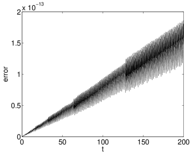
(a) (b)

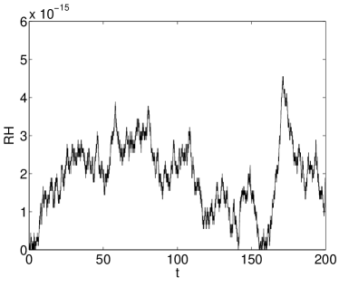
Figure 1: The numerical solution of the sixth order method with $h=0.01$ from $t=0$ to $t=20000$. a Solution error. b Relative energy error

Table 5: The numerical solutions of three AVF methods for example 2

$t=20000$	second order method	fourth order method	sixth order method
$h_{1}=0.02,error(h_{1})$	5.8324 $\times 10^{-3}$	2.3287 $\times 10^{-7}$	9.4389 $\times 10^{-12}$
$h_{2}=0.01,error(h_{2})$	1.4562 $\times 10^{-3}$	1.4554 $\times 10^{-8}$	1.4611 $\times 10^{-13}$
$order$	2.0019	4.0000	6.0135
$max(RH(h_{1}))$	2.5535 $\times 10^{-15}$	2.2204 $\times 10^{-15}$	3.6638 $\times 10^{-15}$

Table 6: The convergence order of the sixth order AVF method with different time steps, $h_{1}=0.2,h_{2}=0.1,h_{3}=0.05,h_{4}=0.025,h_{5}=0.0125$

	$\frac{error(h_{1})}{error(h_{2})}$	$\frac{error(h_{2})}{error(h_{3})}$	$\frac{error(h_{3})}{error(h_{4})}$	$\frac{error(h_{4})}{error(h_{5})}$
$t=1$	63.7145	63.9285	63.8679	74.4285
$t=2$	63.7132	63.9320	63.9419	60.7933
$t=3$	63.7142	63.9287	63.9125	66.0209
$t=4$	63.7138	63.9287	63.9132	67.6980
$t=5$	63.7141	63.9298	63.9419	63.3118
$t=200$	63.7162	63.9280	63.9409	62.9838

5.3 Numerical example 3

Third, we consider a nonlinear Hamiltonian system

$$\dot{z}=J^{-1}\nabla H,H(z)=\frac{1}{4}(p^{2}+q^{2})^{2},$$ (22)

$$z=\left(\begin{array}[]{c}p\\ q\end{array}\right),z_{0}=\left(\begin{array}[]{c}1\\ 0\end{array}\right),J=\left(\begin{array}[]{cc}0&1\\ -1&0\end{array}\right),$$

which has the exact solution

$$p(t)=cos(t),$$

$$q(t)=sin(t).$$

We can obtain the sixth order AVF method of (22)

$$\left(\begin{array}[]{c}p_{1}\\ q_{1}\end{array}\right)=\left(\begin{array}[]{c}p_{0}\\ q_{0}\end{array}\right)+\{hI-\frac{h^{3}}{12}A(\begin{picture}(9.0,7.0)(0.0,0.0)\allinethickness{0.65pt} \put(3.0,-1.5){\circle*{2.0}} \put(6.0,6.5){\circle*{2.0}} \put(3.0,14.5){\circle*{2.0}} \put(3.0,-1.5){\line(3,8){3.0}} \put(6.0,6.5){\line(-3,8){3.0}} \end{picture})+\frac{h^{5}}{720}[6A(\begin{picture}(9.0,7.0)(0.0,0.0)\allinethickness{0.65pt} \put(3.0,-1.5){\line(34,80){3.0}} \put(6.0,5.5){\line(-34,80){3.0}} \put(3.0,11.5){\line(34,80){3.0}} \put(6.0,17.5){\line(-34,80){3.0}} \put(3.0,-1.5){\circle*{2.0}} \put(6.0,5.5){\circle*{2.0}} \put(3.0,11.5){\circle*{2.0}} \put(6.0,17.5){\circle*{2.0}} \put(3.0,23.5){\circle*{2.0}} \end{picture})-A(\begin{picture}(9.0,6.0)(-7.0,0.0)\allinethickness{0.65pt} \put(0.0,6.5){\line(-34,80){3.4}} \put(0.0,6.5){\line(34,80){3.4}} \put(-3.0,-1.0){\line(34,80){3.4}} \put(-3.0,-1.0){\line(-34,80){3.4}} \put(-4.0,14.5){\circle*{2.0}} \put(0.0,6.5){\circle*{2.0}} \put(3.0,14.5){\circle*{2.0}} \put(-6.0,6.0){\circle*{2.0}} \put(-3.0,-1.0){\circle*{2.0}} \end{picture})+A(\begin{picture}(6.0,7.0)(0.0,0.0)\allinethickness{0.65pt} \put(3.0,-1.5){\line(34,80){3.4}} \put(6.0,6.5){\line(-34,80){3.4}} \put(3.0,14.5){\line(34,80){3.4}} \put(3.0,14.5){\line(-34,80){3.4}} \put(3.0,-1.5){\circle*{2.0}} \put(6.0,6.5){\circle*{2.0}} \put(3.0,14.5){\circle*{2.0}} \put(6.0,22.5){\circle*{2.0}} \put(0.0,22.5){\circle*{2.0}} \end{picture})-A(\begin{picture}(12.0,7.0)(1.0,0.0)\allinethickness{0.65pt} \put(7.0,-1.5){\line(34,80){3.4}} \put(7.0,-1.5){\line(-34,80){3.4}} \put(10.4,6.5){\line(-34,80){3.4}} \put(7.0,14.5){\line(34,80){3.4}} \put(7.0,-1.5){\circle*{2.0}} \put(10.4,6.5){\circle*{2.0}} \put(3.6,6.5){\circle*{2.0}} \put(7.0,14.5){\circle*{2.0}} \put(10.4,22.5){\circle*{2.0}} \end{picture})-\frac{3}{2}A(\begin{picture}(16.4,7.0)(0.0,0.0)\allinethickness{0.65pt} \put(8.2,6.5){\line(62,80){6.2}} \put(8.2,6.5){\line(-62,80){6.2}} \put(8.2,6.5){\line(0,1){8.0}} \put(8.2,-1.5){\line(0,1){8.0}} \put(8.2,-1.5){\circle*{2.0}} \put(14.4,14.5){\circle*{2.0}} \put(2.0,14.5){\circle*{2.0}} \put(8.2,14.5){\circle*{2.0}} \put(8.2,6.5){\circle*{2.0}} \end{picture})$$

$$-\frac{3}{2}A(\begin{picture}(16.4,7.0)(0.0,0.0)\allinethickness{0.65pt} \put(8.2,-1.5){\line(62,80){6.2}} \put(8.2,-1.5){\line(-62,80){6.2}} \put(8.2,-1.5){\line(0,1){8.0}} \put(2.0,6.5){\line(62,80){6.2}} \put(8.2,-1.5){\circle*{2.0}} \put(14.4,6.5){\circle*{2.0}} \put(2.0,6.5){\circle*{2.0}} \put(8.2,6.5){\circle*{2.0}} \put(8.2,14.5){\circle*{2.0}} \end{picture})+3A(\begin{picture}(16.4,7.0)(0.0,0.0)\allinethickness{0.65pt} \put(8.2,-1.5){\line(62,80){6.2}} \put(8.2,-1.5){\line(-62,80){6.2}} \put(14.4,6.5){\line(-30,80){3.0}} \put(2.0,6.5){\line(30,80){3.0}} \put(8.2,-1.5){\circle*{2.0}} \put(14.4,6.5){\circle*{2.0}} \put(2.0,6.5){\circle*{2.0}} \put(5.2,14.5){\circle*{2.0}} \put(11.2,14.5){\circle*{2.0}} \end{picture})+3A(\begin{picture}(12.0,7.0)(3.8,0.0)\allinethickness{0.65pt} \put(9.8,-1.5){\line(0,1){8.0}} \put(9.8,6.5){\line(34,80){3.4}} \put(9.8,6.5){\line(-34,80){3.4}} \put(6.4,14.5){\line(34,80){3.4}} \put(9.8,-1.5){\circle*{2.0}} \put(9.8,6.5){\circle*{2.0}} \put(13.2,14.5){\circle*{2.0}} \put(6.4,14.5){\circle*{2.0}} \put(9.8,22.5){\circle*{2.0}} \end{picture})]\}F,$$

where $A(\tau)=A(\tau)(\frac{z_{1}+z_{0}}{2})$ are coefficient matrices of $F=\int_{0}^{1}f(\xi z_{1}+(1-\xi)z_{0}))d\xi$, and

$$F=\left(\begin{array}[]{c}F^{1}\\ F^{2}\end{array}\right)=\left(\begin{array}[]{c}\int_{0}^{1}f^{1}(\xi z_{1}+(1-\xi)z_{0}))d\xi\\ \int_{0}^{1}f^{2}(\xi z_{1}+(1-\xi)z_{0}))d\xi\end{array}\right)$$

$$=\left(\begin{array}[]{c}-[((p_{0})^{2}+\frac{1}{3}(p_{1}-p_{0})^{2}+p_{0}(p_{1}-p_{0}))q_{0}\\ +(\frac{1}{2}(p_{0})^{2}+\frac{1}{4}(p_{1}-p_{0})^{2}+\frac{2}{3}p_{0}(p_{1}-p_{0}))(q_{1}-q_{0})\\ +((q_{0})^{2}+\frac{1}{3}(q_{1}-q_{0})^{2}+q_{0}(q_{1}-q_{0}))q_{0}\\ +(\frac{1}{2}(q_{0})^{2}+\frac{1}{4}(q_{1}-q_{0})^{2}+\frac{2}{3}q_{0}(q_{1}-q_{0}))(q_{1}-q_{0})],\\ ((p_{0})^{2}+\frac{1}{3}(p_{1}-p_{0})^{2}+p_{0}(p_{1}-p_{0}))p_{0}\\ +(\frac{1}{2}(p_{0})^{2}+\frac{1}{4}(p_{1}-p_{0})^{2}+\frac{2}{3}p_{0}(p_{1}-p_{0}))(p_{1}-p_{0})\\ +((q_{0})^{2}+\frac{1}{3}(q_{1}-q_{0})^{2}+q_{0}(q_{1}-q_{0}))p_{0}\\ +(\frac{1}{2}(q_{0})^{2}+\frac{1}{4}(q_{1}-q_{0})^{2}+\frac{2}{3}q_{0}(q_{1}-q_{0}))(p_{1}-p_{0}).\end{array}\right)$$

We use the three AVF methods to resolve the problem from $t=0$ to $t=200$.

Fig. 2 shows the solution error and the relative energy error of and the numerical solution of the sixth order method with time evolution in the interval $[0,200]$ respectively. From Fig. 2a we observe that the solution error of the sixth order AVF method shows a slow linear growth. From Fig. 2b we can see that the sixth order AVF method preserves the discrete Hamiltonian very well. So we can conclude that the sixth order AVF method has a good numerical performance for nonlinear Hamiltonian systems in long time.

Table 7 shows the numerical solutions of three AVF methods with time steps $h_{1}=0.02$ and $h_{2}=0.01$. First, we can see that higher order method has higher accuracy. Second, the convergence order of the three AVF methods are 2, 4 and 6 respectively. Third, the relative energy error of the three methods is up to round-off error.

Table 8 shows the convergence order of the sixth order AVF methods with different time steps. We can conclude that the new method is of order six when solving the nonlinear Hamiltonian system.

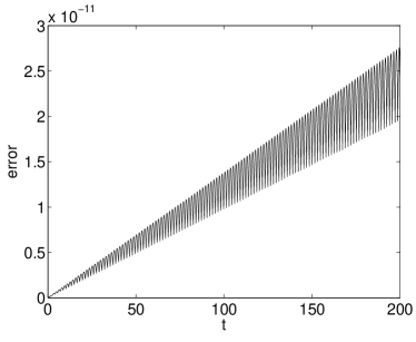
(a) (b)

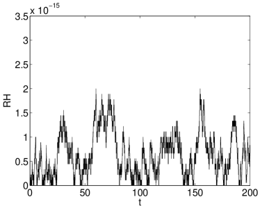
Figure 2: The numerical solution of the sixth order method with $h=0.01$. a Solution error. b Relative energy error

Table 7: The numerical solutions of three AVF methods for example 3

$t=20000$	second order method	fourth order method	sixth order method
$h_{1}=0.02,error(h_{1})$	1.7558 $\times 10^{-2}$	4.5007 $\times 10^{-6}$	1.5495 $\times 10^{-9}$
$h_{2}=0.01,error(h_{2})$	4.3723 $\times 10^{-3}$	2.8137 $\times 10^{-7}$	2.4127 $\times 10^{-11}$
$order$	2.0057	3.9996	6.0050
$max(RH(h_{1}))$	5.2180 $\times 10^{-15}$	1.9984 $\times 10^{-15}$	1.9984 $\times 10^{-15}$

Table 8: The convergence order of the sixth order AVF method with different time steps, $h_{1}=0.2,h_{2}=0.1,h_{3}=0.05,h_{4}=0.025,h_{5}=0.0125$

	$\frac{error(h_{1})}{error(h_{2})}$	$\frac{error(h_{2})}{error(h_{3})}$	$\frac{error(h_{3})}{error(h_{4})}$	$\frac{error(h_{4})}{error(h_{5})}$
$t=1$	61.6174	63.3983	63.8492	63.9435
$t=2$	61.6178	63.3983	63.8497	63.9583
$t=3$	61.6174	63.3982	63.8503	63.9302
$t=4$	61.6167	63.3982	63.8504	63.9213
$t=5$	61.6179	63.3982	63.8515	63.9314
$t=200$	61.6461	63.3975	63.9348	63.4203

5.4 Numerical example 4

Next, we consider the 2-D nonlinear Huygens system

$$\dot{z}=J^{-1}\nabla H,H(z)=p^{2}-q^{2}+q^{4},$$ (23)

$$z=\left(\begin{array}[]{c}p\\ q\end{array}\right),z_{0}=\left(\begin{array}[]{c}0\\ 1.1\end{array}\right),J=\left(\begin{array}[]{cc}0&1\\ -1&0\end{array}\right).$$

We use the sixth order AVF method to resolve the problem from in the interval $[0,500]$. Fig. 3 shows the numerical solution of the sixth order method for the Huygens system with $h=0.005$. From Fig. 3a we can see that the sixth order AVF method can solve the problem very well. From Fig. 3b we can conclude that the Hamiltonian is preserved exactly.

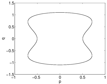
(a) (b)

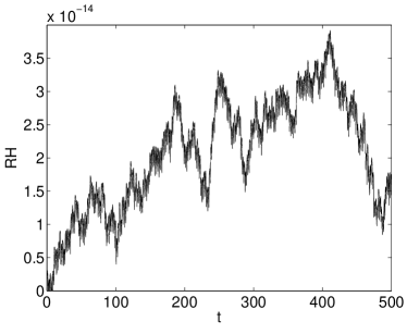
Figure 3: The numerical solution of the sixth order method for the Huygens system with $h=0.005$. a Numerical solution. b Relative energy error

5.5 Numerical example 5

Finally, we consider the pendulum problem, which can be written as a Hamiltonian system

$$\dot{z}=J^{-1}\nabla H,H(z)=\frac{1}{2}p^{2}-cos(q),$$ (24)

$$z=\left(\begin{array}[]{c}p\\ q\end{array}\right),z_{0}=\left(\begin{array}[]{c}0.7\\ 0\end{array}\right),J=\left(\begin{array}[]{cc}0&1\\ -1&0\end{array}\right).$$

We use the sixth order AVF method to resolve the problem in the interval $[0,500]$. Fig. 4 shows the numerical solution of the sixth order method for the Huygens system with $h=0.005$. From Fig. 4a we can see that the sixth order AVF method can solve the problem very well. From Fig. 4b we can conclude that the Hamiltonian is preserved exactly.

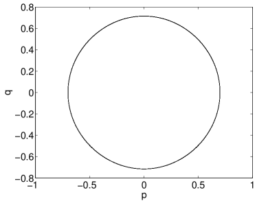
(a) (b)

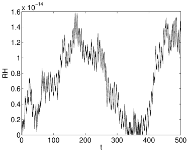
Figure 4: The numerical solution of the sixth order method for the pendulum problem with $h=0.01$. a Numerical solution. b Relative energy error

6 Conclusions

In this paper, we have proposed the concrete formulas of the substitution law for the trees of order $=5$. Based on the new obtained substitution law, we have derived a B-series integrator extending the second order AVF method to sixth order. This approach that we expand a low order B-series integrator into a sixth order integrator can also be used in other geometric B-series integrators naturally, easily and automatically. We have proved that the new method is of order six and it can preserve the energy of Hamiltonian systems. In Ref20 , Faou et al have derived the conditions a B-series method must satisfy in order to be energy-preserving. This new method is a practical integrator of order six. We use the sixth order AVF method to solve linear and nonlinear Hamiltonian systems to test the accuracy and the energy-preserving ability of it. Numerical results confirm the theoretical results.

- (1) Brugnano, L., Iavernaro, F., Trigiante, D.: Hamiltonian boundary value methods(Energy preserving discrete line integral methods). J. Numer. Anal. Ind. Appl. Math. 5,17-37 (2010)
- (2) Bridges, T.J., Reich, S.: Numerical methods for Hamiltonian PDEs. J. Phys. A: Math. Gen. 39, 5287-5320 (2006)
- (3) Butcher, J.C.: The numerical analysis of ordinary differential equations: Runge-Kutta and general linear methods. Wiley, New York (1987)
- (4) Cai, J.X., Wang, Y.S.: Local structure-preserving algorithms for the “good” Boussinesq equation. J. Comp. Phys. 239, 72-89 (2013)
- (5) Celledoni, E., Grimm, V., McLachlan, R.I., McLaren, D.I., O’Neale, D., Owren, B., Quispel, G.R.W.: Preserving energy resp. dissipation in numerical PDEs using the “Average Vector Field” method. J. Comp. Phys. 231, 6770-6789 (2012)
- (6) Celledoni, E., McLachlan, R.I., McLaren, D.I., Owren, B., Quispel, G.R.W., Wright, W.M.: Energy-preserving Runge-Kutta methods. Math. Model. Numer. Anal. 43, 645-649 (2009)
- (7) Chartier, P., Faou, E., Murua, A.: An algebraic approach to invariant preserving integators: the case of quadratic and Hamiltonian invariants. Numer. Math. 103, 575-590 (2006)
- (8) Chartier, P., Hairer, E., Vilmart, G.: A substitution law for B-series vector fields. INRIA report, No. 5498 (2005)
- (9) Chartier, P., Hairer, E., Vilmart, G.: Numerical integration based on modified differential equation. Math. Comp. 76, 1941-1953 (2007)
- (10) Chartier, P., Lapôtre, E.: Reversible B-series. INRIA report, No. 1221 (1988)
- (11) Chen, Y., Sun, Y.J., Tang, Y.F.: Energy-preserving numerical methods for Landau-Lifshitz equation. J. Phys. A: Math. Theor. 44, 295207 (2011)
- (12) Feng, K.: Collected Works of Feng Kang II. National Defence Industry Press, Beijing (1994)
- (13) Faou, E., Hairer, E., Pham, T.-L.: Energy conservation with non-Symplectic methods: examples and counter-examples. BIT Numer. Math. 44, 699-709 (2004)
- (14) Feng, K., Qin, M.Z.: Symplectic Geometric Algorithms for Hamiltonian Systems. Springer/Zhejiang Science and Technology Publishing House, Berlin/Hangzhou (2010)
- (15) Gonzalez, O.: Time integration and discrete Hamiltonian systems. J. Nonlinear Sci. 6, 449-467 (1996)
- (16) Hairer, E.: Energy-preserving variant of collocation methods. J. Numer. Anal. Ind. Appl. Math. 5, 73-84 (2010)
- (17) Hairer, E., Lubich, C., Wanner, G.: Geometric Numerical Integration: Structure Preserving Algorithms for Ordinary Differential Equations. Springer, Berlin (2002)
- (18) Hairer, E., Norsett, S.P., Wanner, G.: Solving Ordinary Differential Equations I, Nonstiff Problems (2nd Edition). Springer, Berlin (1993)
- (19) Hairer, E., Wanner, G.: On the Butcher group and general multi-value methods. Computing 13, 1-15 (1974)
- (20) Iavernaro, F., Trigiante, D.: High-order symmetric schemes for the energy conservation of polynomial Hamiltonian problems. J. Numer. Anal. Ind. Appl. Math. 4, 87-101 (2009)
- (21) Marsden, J.E., Patrick, G.W., Shkoller, S.: Mulltisymplectic geometry, variational integrators, and nonlinear PDEs. Comm. Math. Phys. 199, 351-395 (1998)
- (22) Matsuo, T.: High-order schemes for conservative or dissipative systems. J. Comput. Appl. Math. 152, 305-317 (2003)
- (23) McLachlan, R.I., Quispel, G.R.W., Robidoux, N.: Geometric integration using discrete gradients. Phil. Trans. R. Soc. A. 357, 1021-1045 (1999)
- (24) Qin, H., Zhang, S.X., Xiao, J.Y., Liu, J., Sun, Y.J., Tang, W.M.: Why is Boris algorithm so good?. Phys. Plasmas 20, 084503 (2013)
- (25) Quispel, G.R.W., McLaren, D.I.: A new class of energy-preserving numerical integration methods. J. Phys. A: Math. Theor. 41, 045206 (2008)
- (26) Sanz-Serna, J.M., Calvo, M.P.: Numerical Hamiltonian Problems. Chapman and Hall, London (1994)
- (27) Sun, J.Q., Qin, M.Z.: Multi-symplectic methods for the coupled 1D nonlinear Schrödinger system. Comp. Phys. Comm. 155, 221-235 (2003)
- (28) Wang, Y.S., Hong, J.L.: Multi-symplectic algorithms for Hamiltonian partial differential equations. Comm. Appl. Math. Comput. 27, 163-230 (2013)
- (29) Webb, S.D.: Symplectic integration of magnetic systems. J. Comp. Phys. 270, 570-576 (2014)