The distribution of “time of flight” in three dimensional stationary chaotic advection

Abstract

The distributions of “time of flight” (time spent by a single fluid particle between two crossings of the Poincaré section) are investigated for five different 3D stationary chaotic mixers. Above all, we study the large tails of those distributions, and show that mainly two types of behaviors are encountered. In the case of slipping walls, as expected, we obtain an exponential decay, which, however, does not scale with the Lyapunov exponent. Using a simple model, we suggest that this decay is related to the negative eigenvalues of the fixed points of the flow. When no-slip walls are considered, as predicted by the model, the behavior is radically different, with a very large tail following a power law with an exponent close to $-3$.

I Introduction

Mixing in fluids comes with two mechanisms: stirring, which consists in moving the fluid particles as efficiently as possible so as to create high gradients of concentration that are smoothed by molecular diffusion thereafter. Although mixing generally implies turbulent flows, it is now very well-known that chaotic advection enables efficient stirring even when the flow is laminar bib:aref84 ; bib:ottino89 .

Many recent studies, mostly in 2D flows, have shown how mixing in chaotic advection (and more especially the variance decay of a diffusive tracer) is controlled by regions of low stretching rate: in the presence of walls bib:chertkovlebedev03 ; bib:salmanhaynes07 ; bib:gouillartetal07 ; bib:gouillartetal08 , an algebraic decay of the variance, rather than the rapidly predominant exponential decay expected from early numerical simulations is observed bib:pierrehumbert94 ; bib:toussaintetal95 ; bib:antonsenetal96 (associated with the notion of strange eigenmode introduced by Ray Pierrehumbert bib:pierrehumbert94 , see also Giona et al. bib:gionaetal04a ; bib:gionaetal04b ). More recently, in a 3D implementation of the randomized sine map bib:pierrehumbert94 ; bib:pierrehumbert00 (therefore without walls), Ngan and Vanneste bib:nganVanneste2011 suggest that the exponential variance decay is controlled by a few small fluid blobs that remain unstretched for long times.

When dealing with realistic geometries of chaotic three dimensional flows, solving the advection-diffusion equation at high Péclet number is out of reach. Because purely Lagrangian measures are easier to obtain bib:carriere07 , it is natural to search for a characterization of the influence of those regions of poor stretching in the usual tools of dynamical systems. The first idea which comes to mind is to consider Poincaré sections: since the velocity field vanishes at fixed walls, the density of points is lower in the vicinity of the walls than in the bulk; but it is also lower in regions where the velocity component perpendicular to the Poincaré section vanishes. The second simplest idea is to consider the Lyapunov exponents, another classical tool of dynamical systems theory; but, as we will see in the paper, they fail to detect the presence of walls. Jones & Young considered the axial dispersion of a perfect or diffusive tracer along a twisted pipe bib:jonesyoung94 . For instance, they showed that in the case of the perfect tracer, the asymptotic ($t\rightarrow\infty$) shear dispersion $\sigma(t)$ varies like $t\ln t$ in the case of global chaos, whereas it varies like $t^{2}$ in other cases (not global chaos, regular regime or straight pipes); with a simple argument, they related this logarithmic behavior to the presence of walls. Then this measure of chaos is interesting since it can “feel” the presence of walls, while the other tools cited previously cannot. However, it has a major drawback when realistic geometries are under study: indeed, in order to detect the logarithmic behavior, they averaged 10 runs over long times, each run consisting of ensembles of $10^{5}$ particles. They used an analytical solution of their flow, which made the calculation “affordable”. Otherwise, the computational cost would be too high for this parameter to be used systematically. Lobe dynamics bib:romkedaretal90 ; bib:raynalgence95 ; bib:raynalwiggins2006 is a geometrical approach that gives interesting insights on mass exchange between different regions of the chaotic flow, but is quite restricted to 2D flows. More recently, the linked twist map formalism bib:sturman2006 ; bib:sturman2008 , available in 2 and 3D flows, has been proved to be a useful theoretical tool for design principles of efficient mixers available in many technological applications, and was extended for an idealized model of a class of fluid mixing devices of 2D flows to show how scalar decay is related to the presence of boundaries bib:SturmanSpringham2013 . Finally, the purely probabilistic transfer operator approach, available in 2D and 3D flows, determines almost-invariant regions that minimally mix with their surroundings, and, unlike lobe dynamics, is able to detect regions with very small mass leakage bib:froylandpadberg2009 ; the connection with topological chaos was done by Stremler et al. bib:stremleretal2011 .

In the present work, we propose to follow a simpler idea, that is to consider the time of flight, lapse of time spent by a fluid particle between two consecutive crossings of Poincaré sections. Since a fluid particle has a very slow motion when it is located in a region of low stretching, it spends more time between two crossings of the Poincaré section than it would otherwise, resulting in very long times of flight. As a particle wanders almost everywhere in the chaotic region, the histogram of times of flight may be considered as a global rather than local distribution; therefore an expected salient feature is that a satisfactory convergence (especially for the tail of the histogram) is obtained with only a reasonable amount of Poincaré section points (of order 10000, say), much less than for the axial dispersion discussed before. In practice, the histogram of times of flight may be smoothed by considering different initial points in the chaotic region, so as to obtain a reasonable tail for the statistics; note however that the statistics (Lyapunov exponents, Poincaré sections) of each unique trajectory have to be sufficiently converged so that they do not depend on the choice of the initial point.

Using the time of flight is all the more interesting as it is already calculated in preparing the Poincaré section: once a chaotic mixer is under numerical study, it is expected at least to obtain a Poincaré section and see if chaos is global, so as to decide whether the mixer is efficient or not; the knowledge of the time of flight only requires to store the times at which the Poincaré section is crossed, or directly the difference between two consecutive crossing times.

II Time of flight and residence time distributions

The distribution of time of flight has some reminiscences with the distribution of residence time first introduced by Danckwerts bib:danckwerts53 ; bib:danckwerts58a , a very usual tool in chemical engineering sciences; however, as we explain thereafter, they are definitively different.

II.1 Time of flight

As defined previously, the time of flight is the lapse of time between two crossings of Poincaré sections when following a single fluid particle; it is directly connected to dynamical systems theory, since it is linked to the very definition of the Poincaré section. Let $P$ denote the Poincaré map: starting from an initial point located at $\mathbf{x}_{0}$ in the Poincaré section, the ordered set of points is obtained as

$$\mathbf{x}_{n}=P(\mathbf{x_{n-1}}),\ n\geq 0,$$ (1)

where $n$ denotes the ordinal number of the Poincaré section when following the given trajectory (orbit), with an associated ordered set of times of first return, $\tau_{P}$, in a time-continuous dynamical system (see Eckmann and Ruelle, section II.H bib:eckmannruelle85 ):

$$t_{\mathrm{f}}(n)=\tau_{P}(\mathbf{x_{n-1}}),\ n>0\,.$$ (2)

$t_{\mathrm{f}}$ is what we hereafter name “time of flight”, while $\overline{t}_{\mathrm{f}}$ denotes the time of flight averaged over $n$.

Note that we refer to a section in space. This may be contrasted with the time-periodic, 2D case, in which Poincaré sections based on the time-period are often used. Time of flight is intended for steady, 3D flows and, unlike the residence time (defined below), is a purely Lagrangian measure.

Let us calculate the time of flight in an elementary flow like a cylindrical Poiseuille laminar flow: we suppose that two successive Poincaré sections are separated by a length $L$. Because the flow is parabolic, a fluid particle will travel forever on the same straight streamline, at a velocity

$${\bf v}=v_{x}(r){\bf e_{x}},\hbox{ with }v_{x}(r)=U_{\mathrm{max}}\,(1-(r/R)^{2})$$ (3)

where $r$ is the radius at which the fluid particle is initially located, $U_{\mathrm{max}}=2U_{\mathrm{mean}}$ is the (maximum) velocity at the center of the pipe, and $U_{\mathrm{mean}}$ the mean velocity in a transverse section. Then the lapse of time between two crossings of Poincaré sections is always identical, equal to $L/v_{x}(r)$, and the corresponding time of flight distribution is a Dirac function at $t=L/v_{x}(r)$, only depending on the initial location of the given fluid particle.

Finally, note that the notion of time of flight is close to that of waiting time bib:artuso_etal2008 , used in other branches of dynamical system community: the waiting time distribution $\psi_{\cal D}(t)$ over a domain ${\cal D}$ is the probability that a given particle entering ${\cal D}$ remains inside for a duration $t$ (waiting time); like the time of flight, it is a Lagrangian quantity, computed by running a single long trajectory and recording waiting times. We will use the waiting time later in the paper.

II.2 Residence time

As defined by Danckwerts in his seminal paper of 1953 bib:danckwerts53 :
“Suppose some property of the inflowing fluid undergoes a sudden change from one steady value to another: for instance, let the color change from white to red. Call the fraction of red material in the outflow at time $[t]$ later be $F([t])$.” The residence time distribution (RTD) $E(t)$ is the derivative of $F(t)$, as defined in equation (3) of his paper. Note that

$$\int_{0}^{\infty}E(t)\,dt=1,\ \hbox{ and that}\int_{0}^{\infty}t\;E(t)\,dt=t_{\mathrm{mean}}={\cal{V}}/q,$$ (4)

where $\cal{V}$ is the volume of the mixer and $q$ is the flow-rate. Moreover, the residence time is an Eulerian quantity, involving all the fluid (not just a single fluid particle) for the entire mixer (and not for a single slice of it).

Danckwerts calculates RTD for a slice of cylindrical Poiseuille flow of length $L$ (in a non-diffusive case); for $t>L/U_{\mathrm{max}}$ (minimal time needed by the fluid to appear at the outlet), we have:

$$E(t)=\frac{L^{2}}{2U_{\mathrm{mean}}^{2}t^{3}}\ .$$ (5)

Note finally that

$$\int_{t_{\textrm{min}}}^{\infty}E(t)\,dt=1,\quad\text{ and that}\int_{t_{\textrm{min}}}^{\infty}t\;E(t)\,dt=t_{\textrm{mean}}=L/U_{\mathrm{mean}}$$ (6)

One could wonder how to evaluate it in practice in a numerical work: a rather simple idea would be to seed some particles uniformly in the inlet section of the mixer bib:khakharOttino87 ; bib:mezic_etal99 , as for a pulse of concentration. In his other paper cited above bib:danckwerts58a , Danckwerts shows, using a result from Spalding bib:spalding58 , that computing the RTD as a response of a pulse at inlet is only valid for a diffusive tracer. However, following numerically a diffusive particle near a wall is tricky, since the particle is likely to end in the walls…

Residence time is sometimes used as a generic term for many different quantities; in order to avoid confusion, this term will not be used in what follows.

III Mixing systems and numerical approach

In the following, we restrict our study to Stokes flows, and consider flows where chaos is global (no apparent regular regions, i.e. the ergodic region covers the whole fluid domain), which are the cases of practical interest for efficient mixing. In order to investigate the time of flight distribution, we consider five different chaotic mixers, described in details later. The first one is the slipping wall cavity flow, for which an analytical solution exists. For all the other ones (another confined model flow and three realistic open-flow mixers, including the well known Kenics${}^{\textrm{\textregistered}}$ bib:armeniadesetal66 ), the flow-field is solved numerically via finite element method (FEM hereafter).

The determination of time of flight distribution requires long asymptotic evaluations, which, in such complicated geometries, is a hard task. For instance, the loss of particles (that may end in the walls due to intrinsically limited numerical accuracy) must be as small as possible: indeed, particles with very long asymptotic time of flight are those that spend a lot of time near the walls. Moreover, for the three open-flows, our results must not depend on the boundary conditions imposed at the inlet and the outlet. Thus we checked our numerical results on two configurations: first of all, we simulated the first flow (the slipping wall cavity flow) via FEM, and found a perfect match with the results obtained with the analytical solution. In order to have more comparisons, we also used the Kenics${}^{\textrm{\textregistered}}$, for which accurate numerical solutions are available in the literature. The numerical method, together with the method used for computing the Lyapunov exponents, are detailed in Ref. bib:carriere06 ; comparisons with other results (pressure loss, particle loss, etc.) for the Kenics${}^{\textrm{\textregistered}}$ can be found in appendix A: our results agree reasonably well with the existing literature.

In the following, we briefly detail the different configurations and the results obtained in terms of Poincaré sections and Lyapunov exponents. Note that, strictly speaking, “Poincaré section” is somewhat improperly used here, although the extension is classical: for the cavity flows considered here, points with both positive or negative normal velocities are taken into account. For the in-line mixers, intersections are considered at points at cross-sectional planes, spaced according to the basic element, rather than following spatial periodicity, which would have twice this spacing. Except when stated differently, hereafter, Lyapunov exponent means “asymptotic” Lyapunov exponents, by contrast with the so-called “finite-time” Lyapunov exponent we also discuss in the following. We recall that, in a steady 3-D flow, there are three ordered Lyapunov exponents of a Poincaré section $\lambda_{1}\geq\lambda_{2}\geq\lambda_{3}$ satisfying

$$\lambda_{1}+\lambda_{2}+\lambda_{3}=0,$$ (7)

owing to incompressibility and

$$\lambda_{2}=0,$$ (8)

because the dynamical system corresponding to particle fluid trajectory is continuous in time. It is easily deduced that:

$$\lambda_{3}=-\lambda_{1}=-\lambda,$$ (9)

so that only the positive Lyapunov exponent (which may be zero) is required. The Lyapunov exponent of the map $\widehat{\lambda}$ is then given by

$$\widehat{\lambda}=\frac{\lambda}{\overline{t}_{\mathrm{f}}}\,.$$ (10)

III.1 Slipping wall cavity flow

The velocity-field is that of stationary 3-D flow in a cube with slipping boundaries, a case we have used in the past for numerical simulation of the advection-diffusion equation at high Péclet number bib:toussaintetal95 ; bib:toussaintcarriere99 ; bib:toussaintetal00 . We recall that it is the sum of a steady main vortex, $\vec{U}_{1}$, of the Taylor kind whose axis is parallel to a side of the box, and of two counter-rotating steady plane vortices ($\vec{U}_{2}$) with equal amplitudes, see Figure 1$a$.

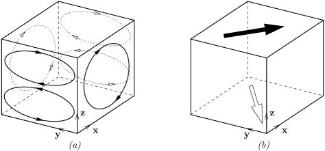
Figure 1: Sketch of the two confined flow-fields: (a) the slipping wall cavity flow (b) the no-slip wall cavity flow (with moving upper and lower walls); the second mimics the first more realistically.

The velocity field is:

$$v_{x} = -U_{1}\sin\pi x\cos\pi z$$ (11)

$$v_{y} = -2\,U_{2}\sin\pi y\cos 2\pi z$$ (12)

$$v_{z} = U_{1}\cos\pi x\sin\pi z+U_{2}\cos\pi y\sin 2\pi z$$ (13)

where the constants $U_{1}$ and $U_{2}$ satisfy the normalization condition $U_{1}^{2}+5U_{2}^{2}/2=1$. We recall that this flow is globally chaotic for $U_{1}\leq 0.25$, and that values of $U_{1}$ such that $U_{1}\leq 0.15$ correspond to cases of global chaos with transadiabatic drift bib:bajermoffatt90 . The case $U_{1}=0.25$ is the flow for which both chaos is global and the Lyapunov exponent is maximum ($\widehat{\lambda}=\ln 7.22$). The corresponding Poincaré section (50,000 points here), calculated in a plane of constant $x$ passing through the center of the box, is reproduced in figure 2.$a$. The empty region near the middle plane corresponds to vanishing of the velocity component perpendicular to the Poincaré section.

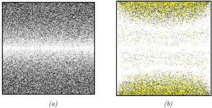
Figure 2: Poincaré sections (plane $(x=0.5)$) for: (a) the slipping wall cavity flow in the case of global chaos $U_{1}=0.25$; (b) the no-slip walls cavity flow: in this case, two Poincaré sections are superimposed, represented by two different colors in the online version.

III.2 No-slip walls cavity flow

In order to check the effect of a no-slip velocity field on the behavior of the time of flight distribution, we propose a second configuration, which mimics the preceding one, but in a more realistic manner: the flow is induced by the stationary motion of the upper and lower walls ($z$ defining the vertical coordinate), co-moving in the $y$-direction and counter-moving in the $x$-direction bib:carriere06 (figure 1(b)). Somehow, it may be seen as a (stationary) three dimensional implementation of the time-periodic 2D cavity flow studied by Leong and Ottino bib:leongottino89 . As for the flow of the preceding section, Lagrangian properties depend on the relative amplitude of the velocity components in the $x$- and $y$-direction; with the same ratio than herein, the chaotic region densely covers the whole domain. In this case, we expect an additional empty region in the Poincaré section at the vicinity of the fixed vertical walls. However, as can be noticed when looking at figure 2.$b$, some more empty regions are visible: two counter-recirculating vortices parallel to the $y$-axis are present rather than the single vortex of the slipping-walls case. It may be inferred that the mixing efficiency of such a flow is lower than for the first one, with a Lyapunov number $\widehat{\lambda}=\ln 3.57$. Note finally that the number of section points we were able to calculate is lower than for the analytical flow: two sections are here superimposed, the first one with 14,734 points, the second one with 10,850, that clearly overlay each other.

III.3 Kenics${}^{\textrm{\textregistered}}$ Mixer

The Kenics${}^{\textrm{\textregistered}}$ mixer is probably the most famous and widely used static mixer. It is composed of a series of internal blades inside a circular pipe of diameter $d$, each blade consisting of a short helix of length $L$ with a twist angle $\phi$. The series is a succession of right- and left-handed blades, arranged alternately so that the leading edge of a given blade is at right angle of the trailing edge of the preceding blade, thus with a spatial period of length $2L$. A commercial model is shown in figure 3.$a$.

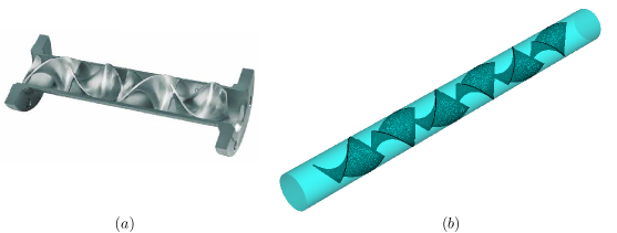
Figure 3: $(a)$ A Kenics${}^{\textrm{\textregistered}}$ KM static mixer supplied by Chemineer, Inc.; $(b)$ Computational geometry.

Hobbs and Muzzio performed simulations in this configuration using a commercial code for both flow simulation and particle tracking bib:hobbsmuzzio97 (see also Ref. bib:hobbsetal98 ), while accurate numerical simulations for a large range of Reynolds number were performed by Byrde and Sawley bib:byrde97 ; bib:byrdesawley99 ; bib:byrdesawley99b . More references of experimental or numerical works are also available in the recent article by Kumar et al. bib:kumaretal08 . In order to use part of the existing results as a check for our own calculations, we used the same parameters as O. Byrde bib:byrde97 , i.e. $L=3d/2$ and $\phi=180^{\mathrm{o}}$.

The geometry used for our FEM simulations is plotted in figure 3.$b$ Although a real mixer would involve about 12 or 16 successive blades, this 6-blades configuration is a good compromise between a realistic mixer and reasonable calculation time.

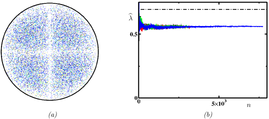
Figure 4: Kenics mixer: (a) Poincaré sections (four sections are superimposed); (b) convergence of the positive Lyapunov exponent with the number of mixing elements $n$; the dot-dashed line is $\ln(2)$.

The Poincaré section (figure 4.$a$) shows a quite homogeneous global chaos away from the walls: four Poincaré sections are superimposed on the plot, containing 2720, 3238, 3191 and 7737 points, respectively, corresponding to different initial locations, which clearly overlay each other.

Note that the Lyapunov exponent converges towards $0.56\approx\ln 1.75$ (figure 4.$b$), that is, a quite lower value than for the baker’s map. This is finally the point on which our result disagree the most with the existing literature. Byrde and Sawley determined values slightly higher than $\ln 2$; however, their calculations were performed in a context of non-negligible inertial effects (Reynolds number $25$ and $100$) which may enhance the resulting stretching: incidentally, the value they predict for $R=100$ is largely higher than the one at $R=25$. Also they dealt with finite time Lyapunov exponents, that depend on the initial location of the particle, thus requiring some far from obvious averaging: At the opposite, the present asymptotic Lyapunov exponents are naturally averaged over the domain and de facto include the probability density function of each point in the Poincaré section. Note finally that our numerical simulations predict a rapid and clear convergence towards $\ln(2)$ for the two following static mixers (figure 6). Thus the value of $\ln 1.75$ for a Stokes flow is indeed a measure of efficiency, and, in the case of creeping flows, mixing in this Kenics configuration is not as efficient as for the baker’s map.

III.4 Multi-level laminating mixer and ”F” mixer

In a previous paper bib:carriere07 , a three-dimensional flow configuration, which tries to mimic as close as possible the baker’s map, was proposed and studied. The corresponding geometry, here in the more realistic variant of an open flow composed of 6 basic “mixing elements”, is given in figure 5.$a$ together with a plot of an iso-surface of velocity modulus for illustrating the separation–stacking process. The design is close to the multi-level laminating mixer (MLLM) proposed by Gray et al. bib:grayetal99 .

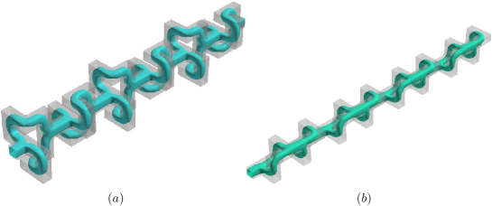
Figure 5: Geometry and iso-surface of velocity modulus plot for a Stokes flow inside: ($a$) the Multi-level laminating mixer (6 elements); ($b$) the ”F” mixer of Chen and Meiners bib:chenmeiners04 (8 elements).

The successive elements are inverted so as to break the symmetry of the flow and eliminate small residual islands in the Poincaré section. Such a mixer configuration is sometimes named “baker’s flow” bib:lesteretal2012 ; bib:lesteretal2013 . Because the results, in the present context, are very similar, we present simultaneously the case of the “F” mixer of Chen and Meiners bib:chenetal09 ; bib:chenmeiners04 , whose geometry is given in figure 5.$b$.

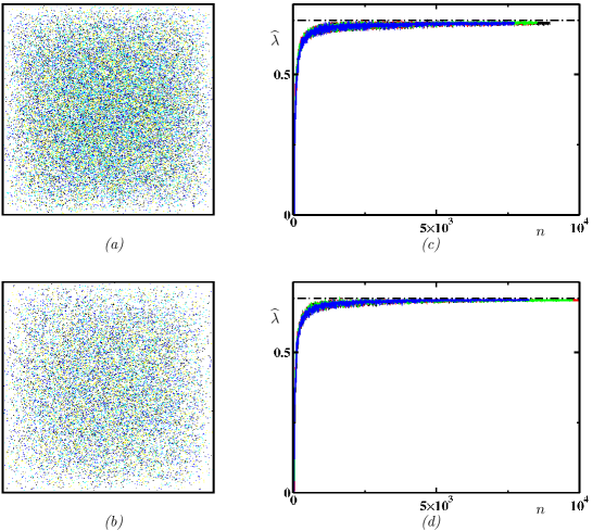
Figure 6: Left: Poincaré sections (four sections are superimposed) for ($a$) the Multi-level laminating mixer; ($b$) the “F” mixer. Right: convergence of the positive Lyapunov exponent with the number of mixing elements $n$ for ($c$) the Multi-level laminating mixer; ($d$) the “F” mixer.

It may appear somewhat surprising to retrieve that, as alluded before, the Lyapunov exponent is $\ln 2$ within the accuracy of the numerical method (figures 6.$c$ and 6.$d$). Thus, despite the walls, these two mixers succeed in approaching the mean behavior of the baker’s map. Figure 6 shows Poincaré sections for each mixer: four Poincaré sections having 8959, 8387, 8508 and 7716 points are superimposed in Fig. 6.$a$ and sections with 5000, 4989, 4877 and 4121 points in 6.$b$.

IV Time of flight

As defined earlier, time of flight $t_{\mathrm{f}}$ is the time spent by a single particle between two consecutive intersections with the Poincaré plane. We denote by $n$ the ordinal number of Poincaré section when following the given trajectory, and by $\overline{t}_{\mathrm{f}}$ the time of flight averaged over $n$. Figure 7$a$ shows a typical plot of the behavior of the “reduced time of flight” $t_{\mathrm{f}}/\overline{t}_{\mathrm{f}}$ as a function of $n$ in a mixer with fixed no-slip boundaries (here the multi-level laminating mixer).

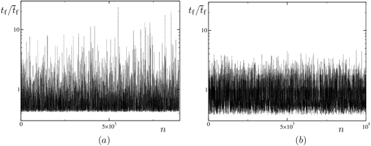
Figure 7: Non-dimensional time of flight, $t_{\mathrm{f}}/\overline{t}_{\mathrm{f}}$, versus the ordinal number of Poincaré section points, $n$ for a unique trajectory, corresponding to: $(a)$ one of the Poincaré sections in figure 6.$a$ (multi-level laminating mixer); $(b)$ the trajectory in figure 2.$a$ (slipping-walls cavity flow).

As expected for a chaotic trajectory, it exhibits highly random behavior. Note the use of a logarithmic scale for the vertical axis, so as to allow for extreme events (large departures from the mean), corresponding to situations where the particle is trapped for a long time in the near vicinity of walls, before escaping to the core of the flow. In this respect, it is clear that the statistics in cases $a$ and $b$ (respectively no-slip and slipping boundaries) are dissimilar. As a consequence, the tails of the distributions of time of flight are expected to be quite different depending on the presence or not of no-slip walls: in figure 8, we compare the probability density functions (pdf) of the reduced time of flight $t_{\mathrm{f}}/\overline{t}_{\mathrm{f}}$ for the two preceding cases; the two pictures are plotted with the same lin-log scale.

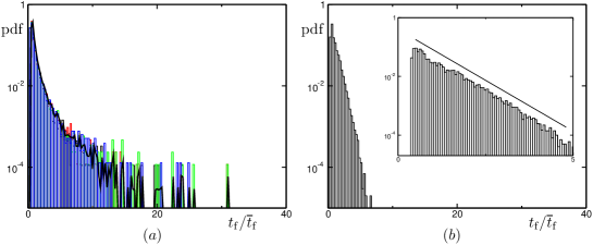
Figure 8: Distribution of reduced time of flight for: $(a)$ the multi-level laminating mixer; $(b)$ the slipping-walls cavity flow. In the former case, four histograms corresponding to the four trajectories of figure 6.$a$ are superimposed; the thick black solid line represents the distribution averaged over these four histograms. In the second case, the distribution is shown at another scale, so as to see clearly the exponential decay.

As one would expect in a globally chaotic flow, the distribution of time of flight indeed reveals an exponential decay with $t_{\mathrm{f}}/\overline{t}_{\mathrm{f}}$ in the slipping wall cavity flow, but the result is completely different concerning the no-slip walls flow. Thus we will consider those two cases separately thereafter.

IV.1 No-slip boundaries

IV.1.1 Theoretical model

In order to understand this non-exponential behavior in the presence of walls, we propose to mimic the trajectory of a single fluid particle in such chaotic flows as follows:

• the flow in an element of the mixer is modeled by a non-chaotic flow, here possessing no-slip boundaries;

• the effect of global chaos on the trajectory of the fluid particle is modeled by random reinjection at the entry to the next element with a non uniform probability distribution, that takes into account the fact that the particle randomly samples the whole section, but less near the walls;

• in order to preserve mass conservation, the probability density function of the location of reinjection is taken proportional to the velocity rate.

For instance, a mixing element of the Kenics${}^{\textrm{\textregistered}}$ is replaced by a piece of cylindrical pipe, or the no-slip walls cavity flow is modeled by a piece of plane Couette flow; in each element of the model, the trajectory is thus a straight segment following a streamline of the flow, while the location of the particle changes at each new element. The shape of the distribution can be further explained as follows: during a lapse of time $dt$, less particles of the flow cross the section near the walls than in the core where the velocity is maximum; therefore the probability density for the single particle to cross the section at a given point must also follow this flux of particles. This last property was also used in a 3D-model of chaotic flow with sources and sinks in a Hele-Shaw cell, where the flow was calculated first in 2D, and the $z$-dependence was modeled by a parabolic reinjection rate from the source, with surprisingly good agreement between the model and 3D-calculations bib:raynaletal2013 . Using these model flows, it is possible to obtain an analytical expression for the distributions of time of flight. We present hereafter the calculations in a cylindrical pipe (Poiseuille flow, see figure 9), with velocity-field given by equation (3).

Figure 9: Poiseuille flow: the time of flight is calculated with Poincaré sections being separated by a length $L$.

The calculation for the plane Couette flow is developed in Appendix B.

Let $G(t)$ be the probability density to have a time of flight of duration $t$ for an element of length $L$; $G(t)dt$ is therefore the probability to have a time of flight in between $t$ and $t+dt$. Given

$$t=L/v_{x}(r)\;,$$ (14)

$t$ depends only on $r$, so this probability is equal to that of having a particle between $r$ and $r+dr$, with $r$ the radius related to time of flight $t$ by equation (14). Thus the probability of having a particle reinjected in between $r$ and $r+dr$ is such that

$$G(t)dt\propto v_{x}(r)2\pi rdr.$$ (15)

From equations 3 and 14, we have:

$$1-(r/R)^{2}=\frac{L}{U_{\mathrm{max}}\,t}$$ (16)

that can be differentiated into

$$-2r/R^{2}dr=-\frac{L}{U_{\mathrm{max}}\,t^{2}}dt.$$ (17)

We finally obtain:

$$G(t)\propto t^{-3}.$$ (18)

We also obtain a $t^{-3}$ tail in the case of plane Couette flow (see Appendix B), and plane Poiseuille flow (calculation not given here).

IV.1.2 Time of Flight histograms

Figure 10: Distribution of time of flight for: $(a)$ the no-slip walls cavity flow; $(b)$ the Kenics${}^{\textrm{\textregistered}}$ mixer; $(c)$ the multi-level laminating mixer; $(d)$ the ”F” mixer. The histogram is averaged over two trajectories (used to plot figure 2.$b$) in plot $(a)$, and those in plots $(b$–$d)$ are averaged over four trajectories (similarly those used to plot the corresponding Poincaré sections); in all cases the smallest count is the inverse of the number of times of flights calculated, of the order of: $(a)$: $4\,10^{-5}$; $(b)$: $6\,10^{-5}$; $(c)$: $3\,10^{-5}$; $(d)$: $5\,10^{-5}$. The dotted line stands for the $t^{-3}$ power law.

In order to compare the predictions from our model with our numerical results, we plot in figure 10 the histograms of time of flights (calculated together with the Poincaré sections shown in figures 2$b$, 4.$a$, and 6.$a$-$b$ respectively), in log-log scales, for all the mixers with no-slip boundaries described in section III (namely, the no-slip walls cavity flow, the multi-level laminating mixer, the “F” mixer, and the Kenics${}^{\textrm{\textregistered}}$ mixer): even in the case of the no-slip walls cavity, which may be considered as different from the three more realistic static mixers, the histograms exhibit a power law with an exponent close to $-3$. Although the details of the flow may influence the short time statistics, and therefore, because of mass conservation, the amplitude of the tail, note that those histograms have a very similar shape, with close values of absolute amplitude of the algebraic tails. The fact that we recover the same type of behavior for the distribution of time of flight from numerical results and with our model favors the hypothesis that the shape of the distribution of time of flight is a signature of the presence (or not) of solid fixed walls inside the flow.

IV.2 The slipping-walls (TCR) flow

As shown in figure 7.$b$, the tail of the histogram is clearly exponential, as one would expect in a fully chaotic flow; however, it does not scale with the Lyapunov exponent. Indeed, the Lyapunov exponent can be seen as a “mean stretching rate”, that takes into account regions of high or low stretching visited by the fluid particle, while the tails of histograms correspond to long time of flights, connected to trapping of the particle in regions of low stretching rates. Thus the reason for this exponential decay is not completely entangled in the chaotic nature of the flow, but rather may be explained by the presence of hyperbolic fixed points: it requires infinite time for a point located exactly on the stable manifold of an hyperbolic fixed point to reach this fixed point; thus it may take arbitrary long time for a fluid particle very close to the stable manifold to reach the vicinity of the fixed point before escaping along the unstable manifold. Those “trappings” along a stable manifold, although scarce, may lead to those rare long time events for the time of flight. Simulations available as supplementary material bib:carriere02a ; bib:carriere02b support this hypothesis.

IV.2.1 Theoretical model

If long times of flight are due to a trapping near a fixed point of the flow, then distributions of times of flight $t_{\mathrm{f}}$ have the same long time behavior as waiting times $\tau$ (defined at the end of paragraph II.1) in a domain around this fixed point. Similarly to the case of flows with walls, we propose a model flow that evaluates the waiting time in the vicinity of a fixed point, constructed as follows:

• the flow around a fixed point is modeled by a non-chaotic flow in a domain ${\cal D}=(-L\leq x\leq 0)\times(r\leq R)$, here possessing a hyperbolic fixed point, like depicted in figure 11;

• Chaos is modeled by a random reinjection in the plane $(x=-L)$, with reinjection probability distribution proportional to the local velocity rate.

Figure 11: Flow in the vicinity of an hyperbolic point (located here at $(x=r=0)$). We define a domain ${\cal D}=(-L\leq x\leq 0)\times(r\leq R)$ around this fixed point; the waiting time in ${\cal D}$, denoted by $\tau$, is the time it takes to move from the plane $(x=-L)$ up to the cylinder $(r=R)$.

Using this model, we can first calculate the waiting time of a given fluid particle, then obtain the corresponding distribution.

Waiting time $\tau$ of a particle with given entrance location $r=r_{0}$: in the domain $\cal{D}$, the velocity field is well-described by the equations

$$v_{x} = -\lambda x$$ (19)

$$v_{r} = \lambda r/2\,.$$ (20)

Consider an individual particle that enters the domain ${\cal D}$ at $t=0$ at point $(x_{0},r_{0})$, and leaves it at $t=\tau$ at point $(x(\tau),r(\tau))$. Using the boundary conditions $x_{0}=-L$ and $r(\tau)=R$, and equations (19) and (20), we obtain:

$$x(\tau) = -L\,\exp(-\lambda\,\tau)$$ (21)

$$R = r_{0}\,\exp(\lambda\tau/2)$$ (22)

so that $\tau$ is well defined by the knowledge of $r_{0}$ using equation (22).

Distribution of waiting times in the domain ${\cal D}$: let $\psi_{{\cal D}}(\tau)$ be the probability density to have a waiting time $\tau$, and $\psi_{{\cal D}}(\tau)d\tau$ the probability to have a waiting time in between $\tau$ and $\tau+d\tau$. Thus $\psi_{{\cal D}}(\tau)$ verifies, for all particles entering the domain at $x_{0}=-L$ through the circlet between $r=r_{0}$ and $r=r_{0}+dr_{0}$:

$$\psi_{{\cal D}}(\tau)\,d\tau\propto v_{x}|_{{}_{x=-L}}\,2\pi r_{0}\,dr_{0}\,;$$ (23)

from equation (19), and using $dr=(\lambda/2)\,rd\tau$ (from equation (20)), we obtain

$$\psi_{{\cal D}}(\tau)\propto L\lambda^{2}\pi\,r_{0}^{2},$$ (24)

and finally, from equation (22)

$$\psi_{{\cal D}}(\tau)\propto\pi R^{2}\,L\,\lambda^{2}\exp(-\lambda\tau).$$ (25)

Note that the same analysis, carried on particles that leave $\cal{D}$ at $r=R$, changes equation (23) into

$$\psi_{{\cal D}}(\tau)\,d\tau\propto v_{r}|_{{}_{r=R}}\,2\pi R\,dx\,,$$ (26)

which, using equations (21) and (19), naturally leads to the same result as in equation (25).

Times of flights: as explained before, we are mainly interested in the long-range decay of $t_{\mathrm{f}}$ (long times of flights), for which we can consider that $t_{\mathrm{f}}\sim\tau$. Thus the time of flight $t_{\mathrm{f}}$ should also have an exponential probability distribution, scaling with negative eigenvalue of fixed point:

$$G(t)\propto\exp(-\lambda t)\,.$$ (27)

IV.2.2 Time of flight histograms

In the model above we have shown that the time of flight distribution in the presence of a single hyperbolic point should decay exponentially, following the negative eigenvalue of this given fixed point. However, in the whole flow, there are many different fixed points, associated with many different negative eigenvalues. We could wonder therefore what the time of flight histograms will look like.

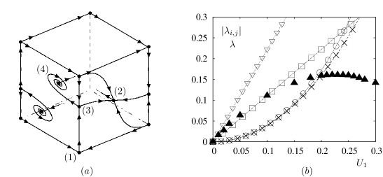
Figure 12: $(a)$: sketch of fixed points in the case of global chaos $U_{1}=0.25$. Fixed points are marked with a filled circle and stable/unstable manifolds are indicated with arrows; for“non-trivial” manifolds, not located on the sides of the cubes, only a very small piece is drawn, ended by a dashed line. Fixed points belonging to the rear sides are omitted for sake of clarity, and may be deduced from symmetry arguments. A fixed point denoted by $(i)$ ($i=1,2,3$ or $4$) on the figure has eigenvalues named $\lambda_{i,j}$ thereafter. $(b)$: absolute values of negative eigenvalues of fixed points for $U_{1}\leq 0.3$ from appendix C, together with the Lyapunov exponents of the flow. For sake of clarity, only those nearer to zero are shown in the figure. ($\blacktriangle$): Lyapunov exponent $\lambda$; ($\times$): $\lambda_{3,1}$; ($\square$): $\lambda_{4,3}$; ($\triangledown$): $\lambda_{3,2}$; ($\circ$): $\lambda_{2,3}$.

The locations and eigenvalues of the fixed points of the TCR flow are calculated in appendix C. A sketch showing those stagnation points in the case of global chaos $U_{1}=0.25$ is given in figure 12$a$: there are 18 stagnation points, all located on the boundary of the cavity, each with one or two directions of stability (possibly of the spiral kind, i.e. associated with complex conjugate eigenvalues). Note that those fixed points exist for all cases studied here ($U_{1}\leq 0.25$), although their location may change for points of type $(3)$ and $(4)$. For most of the cases studied here ($U_{1}\leq 0.25$), as seen in figure 12$b$, the negative eigenvalues nearer to zero are such that

$$0>\lambda_{3,1}\approx\lambda_{2,3}>\lambda_{4,3}>\lambda_{4,1}\,.$$ (28)

Figure 13: Distribution of time of flight for: $(a)$ $U_{1}=0.02$; $(b)$ $U_{1}=0.05$; $(c)$ $U_{1}=0.15$; $(d)$ $U_{1}=0.25$. The symbols correspond to fits with negative eigenvalues; ($\times$): $\lambda_{3,1}$; ($\square$): $\lambda_{4,3}$; ($\triangledown$): $\lambda_{4,1}$.

In the case of global chaos $U_{1}=0.25$ (without transadiabatic drift nor elliptic fixed points), if all hyperbolic points give rise to an exponential decay, then at long times, only the decay with the negative eigenvalue nearer to zero (the one with the slower decay) should be visible. This is exactly what is observed in figure 13$d$, where the decay scales with $\lambda_{3,1}$ (equation (28)).

When transadiabatic drift is present (here for $U_{1}\leq 0.15$), the trajectory of a given particle is almost closed (because the flow is almost regular), so that two successive intersection points $\mathbf{x_{n-1}}$ and $\mathbf{x}_{n}$ in the Poincaré section, linked by equation (1), are very near to each other. This means that a fluid particle remains for a long time in a given region of the flow (where it “visits” some given fixed points), before visiting another region (associated with other fixed points). After very long times it has visited the whole domain, and it is necessary to make statistics over a very large number of Poincaré intersection points (here about $10^{6}$) for a reasonable convergence. As seen in figures 13.$a-c$, in that case the statistics are rather different than what is observed for $U_{1}=0.25$ (figure 13.$d$): the decay is still exponential, but not governed by a single eigenvalue (different slopes are visible in the log-lin plots). This particular behavior is all the more pronounced as $U_{1}$ is small (and the transadiabatic drift phenomenon is important). Moreover, the long time decay does not scale with the smallest negative exponent $\lambda_{3,1}$, but rather with $\lambda_{4,3}$, even with $\lambda_{4,1}$ for very small values of $U_{1}$. This could be explained by the fact that the particle spends longer time in regions visiting the spiraling points of type $(4)$ (figure (12.$a$)) than in the rest of the domain. Finally, note that the shortest times of flight seem to be rather governed by the smallest eigenvalue $\lambda_{3,1}$ for all histograms corresponding to $U_{1}\leq 0.2$ (also on those not shown here).

V Summary and conclusion

In this article we have studied different 3D chaotic stationary mixers with global chaos (no apparent regular regions nor KAM tori), and characterized them in terms of Poincaré sections and Lyapunov exponents. In the case of real mixers, the Lyapunov exponent fails in detecting the presence of solid walls, while the Poincaré sections do not allow to decide between walls or lines of zero normal-velocity. We have proposed to use the histograms of time of flight (lapse of time between two crossings of consecutive Poincaré sections) to study 3D chaotic systems; this tool costs basically nothing more than the calculation of the Poincaré section of the flow. The time of flight results from a single fluid particle that wanders in the whole chaotic region. However, the tail of the distribution (long times of flight) results from regions where the fluid particle remains locally trapped for a while, like in the vicinity of fixed walls, or in regions of poor stretching.

In our numerical investigations, the histograms of time of flight reveal two very different behaviors, depending on whether the chaotic mixer possesses walls or not: whenever fixed solid boundaries are present, a very large tail with a $t^{-3}$ power law decay is observed, while we obtain an exponential law decay in the model case with slipping boundaries. We have proposed a simple model which relates this power law behavior to the presence of walls in the first case; in the case of slipping boundaries, the model shows that the exponential decay is governed by the negative eigenvalues of fixed points of the flow nearer to zero, as shown also by the numerical simulations.

Note finally that, because mixing is also limited in the end by regions where stirring is poor, the shape of time of flight distributions could be somehow related to mixing efficiency, with an algebraic tail when scalar variance decays algebraically, and an exponential tail when scalar variance decays exponentially.

Appendix A Numerical details for the Kenics mixer

Because Lagrangian tracking requires great accuracy, we used 368,951 pressure nodes and 2,770,011 velocity nodes (Eulerian quantities would be satisfactorily obtained with a much lower resolution).

A.1 Inlet and outlet boundary conditions

An important issue in open flows is the imposed boundary conditions at the inlet and the outlet. Firstly, instead of the imposed pressure drop between inlet and outlet, we use a zero pressure drop and add a prescribed volume forcing term to momentum equations in a small part of the domain near the inlet. This produces the same flow as an imposed pressure drop (Ref. bib:carriere07 ). Secondly, rather than using periodic conditions on the velocity field, we imposed zero azimuthal and radial components and a Neumann condition on the axial component at both inlet and outlet. Then we checked that, owing to the short characteristic length for establishing a Stokes flow, the values obtained for the axial components of the velocity at the outlet only slightly deviate from the ones at inlet: this is true to a relative error less than $0.5$ ‰, which is small enough to avoid negative effects on long time integration of trajectories.

A.2 Pressure drop

The pressure drop, or more properly speaking, the hydraulic resistance is an unavoidable point of comparison. Kumar et al. bib:kumaretal08 give some review of experimental and numerical correlations with the Reynolds number from the literature. Following the usual trend, we compute the ratio $K$ between the hydraulic resistance of the mixer and that of a circular pipe with equal diameter, flow rate and length. Even for vanishing Reynolds numbers, there is a large scattering in the results, typically $4.86$ in Ref. bib:grace71 to $7$ in Ref. bib:pahlmuschelknautz80 , while Byrde and Sawley obtained $3.59$. Here we obtained $K=4.67$: given that the depth of the blade is 2 % of the pipe diameter (rather 5–10 % in the industrial configuration and $0$ for Byrde and Sawley simulations), this is in accordance with the discussion in Ref. bib:byrde97 on the importance of the blade depth on the hydraulic resistance.

A.3 Particle tracking

Figure 14 shows colored particle tracking, i.e. the distribution of marked particles in successive planes located at the end of each six elements (together with the leading edge of the first element).

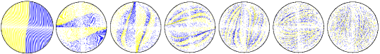
Figure 14: Fluid particles distribution in cross-planes located at, from left to right, the leading edge of the first elements and the end of each of the six elements for the Kenics mixer (figure 3).

The figure may be compared favorably to the ones presented in Ref. bib:byrde97 for a Reynolds number value of $0.01$ and also to experimental visualizations by Grace bib:grace71 (also reported in Ref. bib:byrde97 and bib:middleman77 ). The striation process appears well reproduced even if the comparison is essentially qualitative, looking like a $2^{n}$ process (where $n$ is the number of mixing elements) as reported in the literature bib:grace71 ; bib:middleman77 ; bib:hobbsmuzzio97 .

A.4 Loss of particles

As previously mentioned, numerical limitations are especially severe in the present case. In a few words (see Ref. bib:carriere06 for more details), usual formulations of the discrete pressure–velocity problem (the so-called $P_{1}$-$P_{2}$ element bib:giraultraviart86 in the present FEM method) in three dimensions require some smoothness properties for the pressure field ($p\in H^{1}(\Omega)$ so that its derivatives must be piecewise square integrable) which cannot be satisfied in the vicinity of a “corner”, for instance. Here, this is obviously the case near the leading edge of a blade, where visualization of the pressure field (not shown here) shows ripples of small amplitude; this is also the case along the entire surface of a blade (a succession of triangles), although this appears less critical. This impacts the satisfaction of incompressibility, and explains why following a trajectory for a sufficiently long time is indeed difficult.

Hobbs and Muzzio reported about 5% loss at the end of a 6-elements geometry, and Byrde and Sawley bib:byrdesawley99 about 1-5 % for the tracking of 20,000 and 262,656 particles, respectively. Here we computed the trajectory of 31,630 particles, and obtained about 0.54 % loss (note however that it depends much on the choice of the initial location of particles).

Appendix B Time of flight distribution in a plane Couette flow

Let us consider the laminar flow between two parallel planes, the upper one moving at constant speed ${\bf U}=U\,{\bf e_{x}}$. The velocity-field is such that (figure 15):

$${\bf v}=v_{x}(z)\,{\bf e_{x}},\hbox{ with }v_{x}(z)=Uz/h,\ \hbox{with }0\leq z\leq h$$ (29)

where $h$ is the distance between the walls.

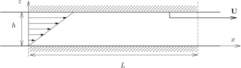
Figure 15: Plane Couette flow: the time of flight is calculated with Poincaré sections being separated by a length $L$.

As before, we let $G(t)$ the probability density to have a time of flight of duration $t$ for a section of length $L$; $G(t)dt$ is therefore the probability to have a time of flight in between $t$ and $t+dt$, which, since ${\bf v}$ depends only on $z$, is equal to the probability of being in between $z$ and $z+dz$, with $z$ the height corresponding to time of flight $t$ such that

$$t=L/v_{x}(z).$$ (30)

Since the reinjection rate is proportional to the velocity, we have

$$G(t)dt\propto v_{x}(z)dz$$ (31)

from equations (30) and (29), we finally obtain:

$$G(t)\propto{t^{-3}}.$$ (32)

Appendix C Fixed points for the slipping wall cavity flow

C.1 location of the fixed points

The locations of the fixed points of the slipping wall cavity flow are given by:

$$\frac{dx}{dt}= -U_{1}\sin\pi x\cos\pi z =0$$ (33)

$$\frac{dy}{dt}= -2U_{2}\sin\pi y\cos 2\pi z =0$$ (34)

$$\frac{dz}{dt}= U_{1}\cos\pi x\sin\pi z+U_{2}\cos\pi y\sin 2\pi z =0$$ (35)

with

$$U_{1}^{2}+\frac{25}{4}U_{2}^{2}=1.$$ (36)

Equations (33) and (34) lead to

$$x=0\hbox{ or } x=1\hbox{ or }z=1/2$$ (37)

$$y=0\hbox{ or } y=1\hbox{ or }z=1/4\hbox{ or }z=3/4.$$ (38)

hence:

1. 8 fixed points located each at a corner of the cube;

2. 2 fixed points located at the center of two opposite walls ($x=1/2$, $y=0$, $z=1/2$ and $x=1/2$, $y=1$, $z=1/2$);

3. If $\xi_{0}=U_{1}/(2U_{2})<1$, which is equivalent to $U_{1}<4/\sqrt{41}\approx 0.625$, there are 4 additional points located on the vertical sides, at $x=0$, $y=0$, $z=1-z_{0}$ and $x=0$, $y=1$, $z=z_{0}$ and $x=1$, $y=1$, $z=1-z_{0}$ and $x=1$, $y=0$, $z=z_{0}$, with $\cos\pi z_{0}=\xi_{0}$;

4. If $\xi_{1}=U_{1}/(\sqrt{2}U_{2})<1$, which is equivalent to $U_{1}<4/\sqrt{66}\approx 0.492$, there are four additional points on two opposite sides of the cubes, at $x=0$, $y=1-y_{1}$, $z=1/4$, and $x=0$, $y=y_{1}$, $z=3/4$ and $x=1$, $y=1-y_{1}$, $z=1/4$ and $x=1$, $y=y_{1}$, $z=3/4$, with $\cos\pi y_{1}=\xi_{1}$.

Fixed points of type $i$ ($i=1,2,3$ or $4$) are indicated by $(i)$ on figure 12. Their eigenvalues are denoted thereafter by $\lambda_{i,j}$

C.2 Eigenvalues of the fixed points

C.2.1 Fixed points located at the corners ($x=\ell$, $y=m$, $z=n$, with $\ell$, $m$, and $n$ equal to $0$ or $1$)

We let $x=\ell+X$, $y=m+Y$ and $z=n+Z$. We obtain the following linearized system for small $X$, $Y$ and $Z$:

$$\frac{dX}{dt} = (-1)^{1+\ell+n}\ U_{1}\pi X$$ (39)

$$\frac{dY}{dt} = (-1)^{1+m}\ 2U_{2}\pi Y$$ (40)

$$\frac{dZ}{dt} = (-1)^{\ell+n}\ U_{1}\pi Z+(-1)^{m}2U_{2}\pi Z$$ (41)

and therefore, 3 real eigenvalues:

$$\lambda_{1,1} = (-1)^{1+\ell+n}\ \pi U_{1}$$ (42)

$$\lambda_{1,2} = (-1)^{1+m}\ 2\pi U_{2}$$ (43)

$$\lambda_{1,3} = (-1)^{\ell+n}\ \pi U_{1}+(-1)^{m}2\pi U_{2}$$ (44)

C.2.2 Fixed points located at the center of two opposite walls ($x=1/2$, $y=m$, $z=1/2$, with $m=0$ or $1$)

We let $x=1/2+X$, $y=m+Y$ and $z=1/2+Z$. We obtain the following linearized system for small $X$, $Y$ and $Z$:

$$\frac{dX}{dt} = U_{1}\pi Z$$ (45)

$$\frac{dY}{dt} = (-1)^{m}\ 2U_{2}\pi Y$$ (46)

$$\frac{dZ}{dt} = -U_{1}\pi X+(-1)^{m+1}\ 2U_{2}\pi Z$$ (47)

and therefore, 3 eigenvalues (2 of which whether real or complex depending on the sign of $U_{2}^{2}-U_{1}^{2}$):

$$\lambda_{2,1} = (-1)^{m}\ \pi 2U_{2}$$ (48)

$$\lambda_{2,2} = (-1)^{1+m}\ \pi\left[U_{2}+(U_{2}^{2}-U_{1}^{2})^{\frac{1}{2}}\right]$$ (49)

$$\lambda_{2,3} = (-1)^{1+m}\ \pi\left[U_{2}-(U_{2}^{2}-U_{1}^{2})^{\frac{1}{2}}\right]$$ (50)

C.2.3 Fixed points located on the vertical sides of the cube ($x=\ell$, $y=m$, $z=Z_{0}$, with $\ell$ or $m=0$ or $1$, and $\cos\pi Z_{0}=(-1)^{1+\ell+m}U_{1}/(2U_{2})$), which exist when $U_{1}<4/\sqrt{41}$

We let $x=\ell+X$, $y=m+Y$ and $z=Z_{0}+Z$. We obtain the following linearized system for small $X$, $Y$ and $Z$:

$$\frac{dX}{dt} = (-1)^{m}\ \left[U_{1}^{2}/(2U_{2})\right]\pi X$$ (51)

$$\frac{dY}{dt} = (-1)^{m}\ 2U_{2}\left[1-U_{1}^{2}/(2U_{2}^{2})\right]\pi Y$$ (52)

$$\frac{dZ}{dt} = (-1)^{m+1}\ 2U_{2}\left[1-U_{1}^{2}/(4U_{2}^{2})\right]\pi Z$$ (53)

and therefore, 3 real eigenvalues:

$$\lambda_{3,1} = (-1)^{m}\ \pi U_{1}^{2}/(2U_{2})$$ (54)

$$\lambda_{3,2} = (-1)^{m}\ \pi 2U_{2}\left[1-U_{1}^{2}/(2U_{2}^{2})\right]$$ (55)

$$\lambda_{3,3} = (-1)^{1+m}\ \pi 2U_{2}\left[1-U_{1}^{2}/(4U_{2}^{2})\right]$$ (56)

C.2.4 Fixed points located on two opposite sides of the cube, which exist when $U_{1}<4/\sqrt{66}$

We let $x=\ell+X$, $y=Y_{1}+Y$, $z=Z_{1}+Z$, with $\ell$ and $n=0$ or $1$, $Z_{1}$ such that $\cos\pi Z_{1}=(-1)^{n}\ \sqrt{2}/2$ and $\cos\pi Y_{1}=(-1)^{1+\ell+n}\ \sqrt{2}U_{1}/(2U_{2})$. We obtain the following linearized system for small $X$, $Y$ and $Z$:

$$\frac{dX}{dt} = (-1)^{1+\ell+n}\ \sqrt{2}/2\,U_{1}\ \pi X$$ (57)

$$\frac{dY}{dt} = (-1)^{n}\ 4U_{2}\ \sin\pi Y_{1}\ \pi Z$$ (58)

$$\frac{dZ}{dt} = (-1)^{n+1}\ U_{2}\ \sin\pi Y_{1}\ \pi Y+(-1)^{\ell+n}\ U_{1}\sqrt{2}/2\pi Z$$ (59)

and therefore, 3 eigenvalues, two of which whether real or complex depending on the sign of $17/8U_{1}^{2}-4U_{2}^{2}$:

$$\lambda_{4,1} = (-1)^{1+\ell+n}\ \pi\sqrt{2}/2\,U_{1}$$ (60)

$$\lambda_{4,2} = (-1)^{\ell+n}\ \pi\left[U_{1}\sqrt{2}/4+(17/8U_{1}^{2}-4U_{2}^{2})^{\frac{1}{2}}\right]$$ (61)

$$\lambda_{4,3} = (-1)^{\ell+n}\ \pi\left[U_{1}\sqrt{2}/4-(17/8U_{1}^{2}-4U_{2}^{2})^{\frac{1}{2}}\right]$$ (62)

References

- (1) H. Aref. Stirring by chaotic advection. J. Fluid Mech., 143:1–21, 1984.
- (2) J.M. Ottino. The Kinematics of Mixing: Stretching, Chaos and Transport. Cambridge University Press, New-York, 1989.
- (3) M. Chertkov and V. Lebedev. Decay of scalar turbulence revisited. Phys. Rev. Lett., 90(3):034501, 2003.
- (4) H. Salman and P. H. Haynes. A numerical study of passive scalar evolution in peripheral regions. Phys. Fluids, 19(6):067101, 2007.
- (5) E. Gouillart, N. Kuncio, O. Dauchot, B. Dubrulle, S.Roux, and J.-L. Thiffeault. Walls Inhibit Chaotic Mixing. Phys. Rev. Let., 99(11):114501, 2007.
- (6) E. Gouillart, O. Dauchot, B. Dubrulle, S. Roux, and J.-L. Thiffeault. Slow decay of concentration variance due to no-slip walls in chaotic mixing. Phys. Rev. E., 78:026211, 2008.
- (7) R. Pierrehumbert. On tracer microstructure in the large-eddy dominated regime. Chaos, Solitons fractals, 4:1091–1110, 1994.
- (8) V. Toussaint, Ph. Carrière, and F. Raynal. A numerical Eulerian approach to mixing by chaotic advection. Phys. Fluids, 7:2587–2600, 1995.
- (9) T. M. Antonsen, Z. Fan, E. Ott, and E. Garcia-Lopez. The role of chaotic orbits in the determination of power spectra of passive scalars. Phys. Fluids, 8(11):3094–3104, 1996.
- (10) M. Giona, A. Adrover, S. Cerbelli, and V. Vitacolonna. Spectral properties and transport mechanisms of partially chaotic bounded flows in the presence of diffusion. Phys. Rev. Lett., 92(11):114101–1–4, 2004.
- (11) M. Giona, S. Cerbelli, and V. Vitacolonna. Universality and imaginary potentials in advection–diffusion equations in closed flows. J. Fluid Mech., 513:221–237, 2004.
- (12) R. T. Pierrehumbert. Lattice modes of advection-diffusion. Chaos, 10(1):61–73, 2000.
- (13) K. Ngan and J. Vanneste. Scalar decay in a three-dimensional chaotic flow. Phys. Rev. E, 83:056306, May 2011.
- (14) Ph. Carrière. On a three-dimensional implementation of the baker’s map. Phys. Fluids, 19:118110, 2007.
- (15) S.W. Jones and W.R. Young. Shear dispersion and anomalous diffusion by chaotic advection. J. Fluid Mech, 1994.
- (16) V. Rom-Kedar, A. Leonard, and S. Wiggins. An analytical study of the transport, mixing and chaos in an unsteady vortical flow. J. Fluid Mech., 214:347–394, 1990.
- (17) F. Raynal and J.N. Gence. Efficient stirring in planar, time-periodic laminar flows. Chem. Eng. Science, 50(4):631–640, 1995.
- (18) F. Raynal and S. Wiggins. Lobe dynamics in a kinematic model of a meandering jet. i. geometry and statistics of transport and lobe dynamics with accelerated convergence. Physica D-Nonlinear Phenomena, 223(1):7–25, NOV 1 2006.
- (19) R. Sturman, J.M. Ottino, and S. Wiggins. The mathematical foundations of mixing: the linked twist map as a paradigm in applications: micro to macro, fluids to solids, volume 22. Cambridge University Press, 2006.
- (20) R. Sturman, S.W. Meier, J.M. Ottino, and S. Wiggins. Linked twist map formalism in two and three dimensions applied to mixing in tumbled granular flows. Journal of Fluid Mechanics, 602:129–174, 2008.
- (21) R. Sturman and J. Springham. Rate of chaotic mixing and boundary behavior. Physical Review E, 87(1):012906, 2013.
- (22) G. Froyland and K. Padberg. Almost-invariant sets and invariant manifolds—connecting probabilistic and geometric descriptions of coherent structures in flows. Physica D: Nonlinear Phenomena, 238(16):1507–1523, 2009.
- (23) M.A. Stremler, S.D. Ross, P. Grover, and P. Kumar. Topological chaos and periodic braiding of almost-cyclic sets. Physical review letters, 106(11):114101, 2011.
- (24) P. V. Danckwerts. Continuous flows systems – distribution of residence times. Chem. Engng. Sci., 2(1):1–13, 1953.
- (25) P. V. Danckwerts. Local residence-times in continuous-flow systems. Chem. Engng. Sci., 9(1):78–79, 1958.
- (26) J.P. Eckmann and D. Ruelle. Ergodic theory of chaos. Rev. Mod. Phys., 57(3):617–656, 1985.
- (27) R. Artuso, L. Cavallasca, and G. Cristadoro. Dynamical and transport properties in a family of intermittent area-preserving maps. Physical Review E, 77(4):046206, 2008.
- (28) D.V. Khakhar, J.G. Franjione, and J.M. Ottino. A case study of chaotic mixing in deterministic flows: the partitioned-pipe mixer. Chemical Engineering Science, 42(12):2909–2926, 1987.
- (29) I. Mezić, S. Wiggins, and D. Betz. Residence-time distributions for chaotic flows in pipes. Chaos: An Interdisciplinary Journal of Nonlinear Science, 9(1):173–182, 1999.
- (30) D.B. Spalding. A note on mean residence-times in steady flows of arbitrary complexity. Chemical Engineering Science, 9(1):74–77, 1958.
- (31) C. D. Armeniades, W. C. Johnson, and T. Raphael. Mixing device. Technical Report 3286992, US Patent, 1966.
- (32) Ph. Carrière. Lyapunov spectrum determination from the FEM simulation of a chaotic advecting flow. Int. J. Num. Meth. Fluids, 50(5):555–577, 2006.
- (33) V. Toussaint and Ph. Carrière. Diffusive cut-off of fractal surfaces in chaotic mixing. Int. J. Bif. Chaos, 9(3):443–454, 1999.
- (34) V. Toussaint, Ph. Carrière, J. Scott, and J.N. Gence. Spectral decay of a passive scalar in chaotic mixing. Phys. Fluids, 12(11):2834–2844, 2000.
- (35) K. Bajer and H.K. Moffatt. On a class of steady Stokes flows with chaotic streamlines. J. Fluid Mech., 212:337–363, 1990.
- (36) C.W. Leong and J.M. Ottino. Experiments on mixing due to chaotic advection in a cavity. J. Fluid Mech., 209:463–499, 1989.
- (37) D. M. Hobbs and F. J. Muzzio. The Kenics static mixer: a three-dimensional chaotic flow. Chem. Eng. J., 67:153–166, 1997.
- (38) D. M. Hobbs, P. D. Swanson, and F. J. Muzzio. Numerical characterization of low Reynolds number flow in the Kenics static mixer. Chem. Eng. Sci., 53(8):1565–1584, 1998.
- (39) O. Byrde. Massively parallel flow computation with application to fluid mixing. PhD thesis, EPF-Lausanne, 1997.
- (40) O. Byrde and M. L. Sawley. Optimization of a Kenics static mixer for non-creeping flow conditions. Chem. Eng. J., 72:163–169, 1999.
- (41) O. Byrde and M. L. Sawley. Parallel computation and analysis of the flow in a static mixer. Comp. Fluids, 28:1–18, 1999.
- (42) V. Kumar, V. Shirke, and K.D.P. Nigam. Performance of kenics static mixer over a wide range of reynolds number. Chem. Eng. J., 139:284–295, 2008.
- (43) B.L. Gray, D. Jaeggi, N.J. Mourlas, B.P. van Drieënhuizen, K.R. Williams, N.I. Maluf, and G.T.A. Kovacs. Novel interconnection technologies for integrated microfluidic systems. Sensors Actuators, 77:57–65, 1999.
- (44) H. Chen and J.-C. Meiners. Topologic mixing on a microfluidic chip. Appl. Phys. Lett., 84(12):2193–2195, 2004.
- (45) D. R. Lester, A. Ord, and B. E. Hobbs. The mechanics of hydrothermal systems: II. Fluid mixing and chemical reactions. Ore Geo. Rev., 12:45–71, 2012.
- (46) D. R. Lester, G. Metcalfe, and M. G. Treffy. Is chaotic advection inherent to porous media flow? Phys. Rev. Let., 111:174101, 2013.
- (47) Z. Chen, M. R. Bown, B. O’Sullivan, J. M. MacInnes, R. W. K. Allen, M. Mulder M. Blom, and R. van’t Oever. Performance analysis of a folding flow micromixer. Microfluidic Nanofluidic, 6:763–774, 2009.
- (48) F. Raynal, A. Beuf, and Ph. Carrière. Numerical modeling of DNA-chip hybridization with chaotic advection. Biomicrofluidics, 7(3):034107, 2013.
- (49) See supplemental material at [movie1.m2v] for the trajectory of a single particle in the case of global chaos : the trajectory is regularly “trapped” in the vicinity of the manifolds associated to fixed points of type (3) and (4), see figure 12.
- (50) See supplemental material at [movie2.m2v] for advection of spot containing a large number of particles in the case of global chaos : spreading is limited in the vicinity of the manifolds associated to fixed points of type (3) and (4), see figure 12.
- (51) C. D. Grace. ‘Static mixing’ and heat transfer. Chem. Proc. Eng., 52:57–59, 1971.
- (52) M.H. Pahl and E. Muschelknautz. Statische mischer und ihre anwendung. Chemie Ingenieur Technik, 52:285–291, 1980.
- (53) S. Middleman. Fundamentals of Polymer Processing. McGraw-Hill, New-York, 1977.
- (54) V. Girault and P.A. Raviart. Finite element methods for Navier–Stokes equations. Springer–Verlag, 1986.