Generalized Labeled Multi-Bernoulli Approximation of Multi-Object Densities

Abstract

In multi-object inference, the multi-object probability density captures the uncertainty in the number and the states of the objects as well as the statistical dependence between the objects. Exact computation of the multi-object density is generally intractable and tractable implementations usually require statistical independence assumptions between objects. In this paper we propose a tractable multi-object density approximation that can capture statistical dependence between objects. In particular, we derive a tractable Generalized Labeled Multi-Bernoulli (GLMB) density that matches the cardinality distribution and the first moment of the labeled multi-object distribution of interest. It is also shown that the proposed approximation minimizes the Kullback-Leibler divergence over a special tractable class of GLMB densities. Based on the proposed GLMB approximation we further demonstrate a tractable multi-object tracking algorithm for generic measurement models. Simulation results for a multi-object Track-Before-Detect example using radar measurements in low signal-to-noise ratio (SNR) scenarios verify the applicability of the proposed approach.

I Introduction

In multi-object inference the objective is the estimation of an unknown number of objects and their individual states from noisy observations. Multi-object estimation is a core problem in spatial statistics [1, 2], and multi-target tracking [3, 4], spanning a diverse range of applications. Important applications of spatial statistics include agriculture/forestry [5, 6, 7], epidemiology/public health [1, 2, 8], communications networks [9, 10, 11], while applications of multi-target tracking include radar/sonar [12, 13, 14], computer vision [15, 16, 17, 18], autonomous vehicles [19, 20, 21, 22], automotive safety [23, 24] and sensor networks [25, 26, 27, 28]. The multi-object probability density is fundamental in multi-object estimation because it captures the uncertainty in the number and the states of the objects as well as the statistical dependence between the objects. Statistical dependence between objects transpires via the data when we consider the multi-object posterior density, or from the interactions between objects as in Markov point processes [29, 30] or determinantal point processes [31, 32, 33].

Computing the multi-object density is generally intractable and approximations are necessary. Tractable multi-object densities usually assume statistical independence between the objects. For example, the Probability Hypothesis Density (PHD) [34], Cardinalized PHD (CPHD) [35], and multi-Bernoulli filters [36], are derived from multi-object densities in which objects are statistically independent. On the other hand, multi-object tracking approaches such as Multiple Hypotheses Tracking (MHT) [37, 38, 13] and Joint Probabilistic Data Association (JPDA) [14] are capable of modeling the statistical dependence between objects. However, MHT does not have the notion of multi-object density while JPDA only has the notion of multi-object density for a known number of objects. A tractable family of multi-object densities that can capture the statistical dependence between the objects is the recently proposed Generalized Labeled Multi-Bernoulli (GLMB) family, which is conjugate with respect to the standard measurement likelihood function[39, 40].

The bulk of multi-object estimation algorithms in the literature, including those discussed above, are designed for the so-called standard measurement model, where data has been preprocessed into point measurements or detections [12, 36, 13, 14, 35]. For a generic measurement model the GLMB density is not necessarily a conjugate prior, i.e. the multi-object posterior density is not a GLMB. This is the case in Track-Before-Detect (TBD) [41, 42, 43, 44, 45, 46], tracking with superpositional measurements [47, 48], merged measurements [49], and video measurements [50],[17]. In general, the multi-object density is numerically intractable in applications involving non-standard measurement models. A simple strategy that drastically reduces the numerical complexity is to approximate the measurement likelihood by a separable likelihood [50] for which Poisson, independently and identically distributed (IID) cluster, multi-Bernoulli and GLMB densities are conjugate. While this approximation can facilitate a trade off between tractability and performance, biased estimates typically arise when the separable assumption is violated.

Inspired by Mahler’s IID cluster approximation in the CPHD filter [35], in this paper we consider the approximation of a general labeled RFS density using a special tractable class of GLMBs. In particular, we derive from this class of GLMBs, an approximation to any labeled RFS density which preserves the cardinality distribution and the first moment. It is also established that our approximation minimizes the Kullback-Leibler divergence (KLD) over this class of GLMB densities. This approximation is then applied to develop an efficient multi-object tracking filter for a generic measurement model. As an example application, we consider a radar multi-object TBD problem with low signal-to-noise ratio (SNR) and closely spaced targets. Simulation results verify that the proposed approximation yields effective tracking performance in challenging scenarios.

The paper is structured as follows: in Section II we recall some definitions and results for Labeled random finite sets (RFSs) and GLMB densities. In Section III we propose the GLMB approximation to multi-object distributions via cardinality, first moment matching and KLD minimization. In Section IV we describe the application of our result to multi-object tracking problems with non-standard measurement models. Simulation results for challenging, low SNR, multi-target TBD in radar scenarios are shown in Section V. Conclusions and future research directions are reported in Section VI.

II Background

This section briefly presents background material on multi-object filtering and labeled RFS which form the basis for the formulation of our multi-object estimation problem.

II-A Labeled RFS

An RFS on a space ${\mathcal{X}}$ is simply a random variable taking values in ${\mathcal{F}}({\mathcal{X}})$, the space of all finite subsets of ${\mathcal{X}}$. The space ${\mathcal{F}}({\mathcal{X}})$ does not inherit the Euclidean notion of integration and density. Nonetheless, Mahler’s Finite Set Statistics (FISST) provides powerful yet practical mathematical tools for dealing with RFSs [51, 34, 3] based on a notion of integration/density that is consistent with measure theory [52].

A labeled RFS is an RFS whose elements are assigned unique distinct labels [39]. In this model, the single-object state space ${\mathcal{X}}$ is the Cartesian product ${\mathbb{X}}{\mathcal{\times}}{\mathbb{L}}$, where ${\mathbb{X}}$ is the kinematic/feature space and ${\mathbb{L}}$ is the (discrete) label space. Let ${\mathcal{L}}:{\mathbb{X}}{\mathcal{\times}}{\mathbb{L}}\rightarrow{\mathbb{L}}$ be the projection ${\mathcal{L}}((x,\ell))=\ell$. A finite subset set ${\mathbf{X}}$ of ${\mathbb{X}}{\mathcal{\times}}{\mathbb{L}}$ has distinct labels if ${\mathbf{X}}$ and its labels $\mathcal{L}(\mathbf{X})\triangleq\{\ell:(x,\ell)\in{\mathbf{X}}\}$ have the same cardinality. An RFS on ${\mathbb{X}}{\mathcal{\times}}{\mathbb{L}}$ with distinct labels is called a labeled RFS [39].

For the rest of the paper, we use the standard inner product notation $\left\langle f,g\right\rangle\triangleq\int f(x)g(x)dx$, and multi-object exponential notation $h^{X}\triangleq\prod_{{}_{x\in X}}h(x)$, where $h$ is a real-valued function, with $h^{\emptyset}=1$ by convention. We denote a generalization of the Kroneker delta and the inclusion function which take arbitrary arguments such as sets, vectors, etc, by

$$\delta_{Y}(X) \triangleq \left\{\begin{array}[]{l}1,{\text{ if }}X=Y\\ 0,{\text{ otherwise}}\end{array}\right.$$

$$1_{Y}(X) \triangleq \left\{\begin{array}[]{l}1,{\text{ if }}X\subseteq Y\\ 0,{\text{ otherwise}}\end{array}\right.$$

We also write $1_{Y}(x)$ in place of $1_{Y}(\{x\})$ when $X=\{x\}$. Single-object states are represented by lowercase letters, e.g. $x$, ${\mathbf{x}}$, while multi-object states are represented by uppercase letters, e.g. $X$, ${\mathbf{X}}$, symbols for labeled states and their distributions are bolded to distinguish them from unlabeled ones, e.g. ${\mathbf{x}}$, ${\mathbf{X}}$, ${\mathbf{\pi}}$, etc, spaces are represented by blackboard bold e.g. ${\mathbb{X}}$, ${\mathbb{Z}}$, ${\mathbb{L}}$, etc. The integral of a function $f$ on ${\mathbb{X}}{\mathcal{\times}}{\mathbb{L}}$ is given by

$$\int f({\bf{\bf x}})d{\bf x}=\sum_{\ell\in{\mathbb{L}}}\int f(x,\ell)dx.$$

Two important statistics of an RFS relevant to this paper are the cardinality distribution $\rho(\cdot)$ and the PHD $v(\cdot)$ [3]:

$$\rho(n) =\frac{1}{n!}\int\boldsymbol{\pi}(\{\mathbf{x}_{1},...,\mathbf{x}_{n}\})d(\mathbf{x}_{1},...,\mathbf{x}_{n})$$ (3)

$$v(x,\ell) =\int\boldsymbol{\pi}({\left\{(x,\ell)\right\}\cup\mathbf{X}})\delta\mathbf{X}$$ (4)

where the integral is a set integral defined for any function $f$ on ${\mathcal{F}}({\mathcal{X}})$ by

$$\int f({\bf{\bf X}})\delta{\bf X}=\sum_{i=0}^{\infty}\frac{1}{i!}\int f(\{\mathbf{x}_{1},...,\mathbf{x}_{i}\})d({\mathbf{x}}_{1},...,\mathbf{x}_{i}).$$

The PHD in (4) and the unlabeled PHD in [39], i.e. the PHD of the unlabeled version, are related by $v(x)=\sum_{\ell\in\mathbb{L}}v(x,\ell)$. Hence, $v(\cdot,\ell)$ can be interpreted as the contribution from label $\ell$ to the unlabeled PHD.

II-B Generalized Labeled Multi-Bernoulli

An important class of labeled RFS is the generalized labeled multi-Bernoulli (GLMB) family [39], which forms the basis of an analytic solution to the Bayes multi-object filter [40]. Under the standard multi-object likelihood, the GLMB is a conjugate prior, which is also closed under the Chapman-Kolmogorov equation [39]. Thus if initial prior is a GLMB density, then the multi-object prediction and posterior densities at all subsequent times are also GLMB densities.

A GLMB is an RFS of ${\mathbb{X}}{\mathcal{\times}}{\mathbb{L}}$ distributed according to

$$\mathbf{\boldsymbol{\pi}}(\mathbf{X})=\Delta(\mathbf{X})\sum_{c\in\mathbb{C}}w^{(c)}(\mathcal{L}(\mathbf{X}))\left[p^{(c)}\right]^{\mathbf{X}}$$ (5)

where $\Delta({\mathbf{X}})\triangleq$$\delta_{|{\mathbf{X}}|}(|{\mathcal{L}}({\mathbf{X}})|)$ denotes the distinct label indicator, ${\mathbb{C}}$ is a discrete index set, and $w^{(c)}$, $p^{(c)}$ satisfy:

$$\sum_{L\subseteq\mathbb{L}}\sum_{c\in\mathbb{C}}w^{(c)}(L) = 1,$$ (6)

$$\int p^{(c)}(x,\ell)dx = 1.$$ (7)

The GLMB density (5) can be interpreted as a mixture of multi-object exponentials. Each term in (5) consists of a weight $w^{(c)}({\mathcal{L}}({\mathbf{X}}))$ that depends only on the labels of ${\mathbf{X}}$, and a multi-object exponential $\left[p^{(c)}\right]^{{\mathbf{X}}}$ that depends on the labels and kinematics/features of ${\mathbf{X}}$.

The cardinality distribution and PHD of a GLMB are, respectively, given by [39]

$$\rho(n) =\sum_{c\in{\mathbb{C}}}\sum_{L\subseteq{\mathbb{L}}}\delta_{n}(|L|)w^{(c)}(L),$$ (8)

$$v(x,\ell) =\sum_{c\in{\mathbb{C}}}p^{(c)}(x,\ell)\sum_{L\subseteq{\mathbb{L}}}1_{L}(\ell)w^{(c)}(L).$$ (9)

A Labeled Multi-Bernoulli (LMB) density is a special case of the GLMB density with one term (in which case the superscript $(c)$ is not needed) and a specific form for the only weight $w(\cdot)$ [39, 53]:

$$w(L) = \prod\limits_{\ell\in{\mathbb{M}}}\left(1-r^{(\ell)}\right)\prod\limits_{\ell\in L}\frac{1_{{\mathbb{M}}}(\ell)r^{(\ell)}}{1-r^{(\ell)}},$$ (10)

where $r^{(\ell)}$ for $\ell\in{\mathbb{M\subseteq L}}$ represents the existence probability of track $\ell$, and $p(\cdot,\ell)$ is the probability density of the kinematic state of track $\ell$ conditional upon existence [39]. Note that the LMB density can always be factored into a product of terms over the elements of $\mathbf{X}$. The LMB density can thus be interpreted as comprising multiple independent tracks. The LMB density is in fact the basis of the LMB filter, a principled and efficient approximation of the Bayes multi-object tracking filter, which is highly parallelizable and capable of tracking large numbers of targets [53, 54].

III Multi-Object Estimation with GLMBs

In this section we discuss the multi-object estimation problem with GLMBs. In particular, in subsection III-A we present a simple approximation through a separable likelihood function which exploits the conjugacy of the GLMB distributions, while in subsection III-B we propose a more principled approach for approximating a general labeled RFS density with a special form GLMB that matches both the PHD and cardinality distribution.

III-A Conjugacy with respect to Separable Likelihoods

A separable multi-object likelihood of the state $\mathbf{X}$ given the measurement $z$ is one of the form [50]:

$$g(z|{\mathbf{X}}) \propto \gamma_{z}^{{\mathbf{X}}}=\prod_{\mathbf{x}\in\mathbf{X}}\gamma_{z}(\mathbf{x})$$ (11)

where $\gamma_{z}(\cdot)$ is a non-negative function defined on $\mathbb{\mathbb{X}}$.

It was shown in [50] that Poisson, IID cluster and multi-Bernoulli densities are conjugate with respect to separable multi-object likelihood functions. Moreover, this conjugacy is easily extented to the family of GLMBs.

Proposition 1.

If the multi-object prior density $\boldsymbol{\pi}$ is a GLMB of the form (5) and the multi-object likelihood is separable of the form (11), then the multi-object posterior density is a GLMB of the form:

$${\mathbf{\boldsymbol{\pi}}}({\mathbf{X}}|z)\propto\Delta({\mathbf{X}})\sum\limits_{c\in{\mathbb{C}}}w_{z}^{(c)}({\mathcal{L}}({\mathbf{X}}))\left[p^{(c)}(\cdot|z)\right]^{{\mathbf{X}}}$$ (12)

where

$$w_{z}^{(c)}(L) = \left[\eta_{z}\right]^{L}w^{(c)}(L)$$ (13)

$$p^{(c)}(x,\ell|z) = p^{(c)}(x,\ell)\gamma_{z}(x,\ell)/\eta_{z}(\ell)$$ (14)

$$\eta_{z}(\ell) = \left\langle p^{(c)}(\cdot,\ell),\gamma_{z}(\cdot,\ell)\right\rangle$$ (15)

Proof:

$$\boldsymbol{\pi}({\mathbf{X}}|z) \propto \gamma_{z}^{{\mathbf{X}}}\boldsymbol{\pi}({\mathbf{X}})$$

$$= \Delta({\mathbf{X}})\sum\limits_{c\in{\mathbb{C}}}w^{(c)}({\mathcal{L}}({\mathbf{X}}))\gamma_{z}^{{\mathbf{X}}}[p^{(c)}]^{{\mathbf{X}}}$$

$$= \Delta({\mathbf{X}})\sum\limits_{c\in{\mathbb{C}}}w^{(c)}({\mathcal{L}}({\mathbf{X}}))\left[\eta_{z}\right]^{{\mathcal{L}}({\mathbf{X}})}\frac{\left[\gamma_{z}p^{(c)}\right]^{\mathbf{X}}}{\left[\eta_{z}\right]^{{\mathcal{L}}({\mathbf{X}})}}$$

$$= \Delta({\mathbf{X}})\sum\limits_{c\in{\mathbb{C}}}w_{z}^{(c)}({\mathcal{L}}({\mathbf{X}}))\left[p^{(c)}(\cdot|z)\right]^{{\mathbf{X}}}.\ \ \ \ \ \ \ \ \ \blacksquare$$

In general, the true multi-object likelihood is not separable, however the separable likelihood assumption can be a reasonable approximation if the objects do not overlap in the measurement space [50].

III-B Labeled RFS Density Approximation

In this subsection we propose a tractable GLMB density approximation to an arbitrary labeled multi-object density $\boldsymbol{\pi}$. Tractable GLMB densities are numerically evaluated via the so-called $\delta$-GLMB form which involves explicit enumeration of the label sets (for more details see [39, 40]). Since there is no general information on the form of $\boldsymbol{\pi}$, a natural choice is the class of $\delta$-GLMBs of the form

$$\mathbf{\boldsymbol{\bar{\pi}}}(\mathbf{X})=\Delta({\mathbf{X}})\sum_{L\in{\mathcal{F}}({\mathbb{L}})}\bar{w}^{(L)}\delta_{L}({\mathcal{L}}(\mathbf{X}))\left[\bar{p}^{(L)}\right]^{\mathbf{X}}$$ (16)

where each $\bar{p}^{(L)}(\cdot,\ell)$ is a density on $\mathbb{X}$, and each weight $\bar{w}^{(L)}$ is non-negative such that $\sum_{L\subseteq\mathbb{L}}w^{(L)}=1$. It follows from (8) and (9) that the cardinality distribution and PHD of (16) are given, respectively, by

$$\bar{\rho}(n) =\sum_{L\subseteq{\mathbb{L}}}\delta_{n}(|L|)\bar{w}^{(L)},$$ (17)

$$\bar{v}(x,\ell) =\sum_{L\subseteq{\mathbb{L}}}1_{L}(\ell)\bar{w}^{(L)}\bar{p}^{(L)}(x,\ell).$$ (18)

Note that such $\delta$-GLMB is completely characterised by the parameter set $\{(\bar{w}^{(L)},\bar{p}^{(L)})\}_{L\in{\mathcal{F}}({\mathbb{L}})}$. Our objective is to seek a density, via its parameter set, from this class of $\delta$-GLMBs, which matches the PHD and cardinality distribution of $\boldsymbol{\pi}$.

The strategy of matching the PHD and cardinality distribution is inspired by Mahler’s IID cluster approximation in the CPHD filter [35], which has proven to be very effective in practice [4, 55, 56]. While our result is used to develop a multi-object tracking algorithm in the next section, it is not necessarily restricted to tracking applications, and can be used in more general multi-object estimation problems.

Our result follows from the following representation for labeled RFS.

Definition 1.

Given a labeled multi-object density $\boldsymbol{\pi}$ on ${\mathcal{F}}({\mathbb{X}}{\mathcal{\times}}{\mathbb{L}})$, and any positive integer $n$, we define the joint existence probability of the label set $\{\ell_{1},...,\ell_{n}\}$ by

$$w(\{\ell_{1},...,\ell_{n}\})\ \ \ \ \ \ \ \ \ \ \ \ \ \ \ \ \ \ \ \ \ \ \ \!\ \ \ \ \ \ \ \ \ \ \ \ \ \ \ \ \ \ \ \ \ \ \$$

$$\triangleq\int\boldsymbol{\pi}(\{(x_{1},\ell_{1}),...,(x_{n},\ell_{n})\})d(x_{1},...,x_{n})$$ (19)

and the joint probability density (on ${\mathbb{X}}^{n}$) of $x_{1},...,x_{n}$, conditional on their corresponding labels $\ell_{1},...,\ell_{n}$, by

$$\!p(\{(x_{1},\ell_{1}),...,(x_{n},\ell_{n})\})\triangleq\frac{\boldsymbol{\pi}(\{(x_{1},\ell_{1}),...,(x_{n},\ell_{n})\})}{w(\{\ell_{1},...,\ell_{n}\})}$$ (20)

For $n=0$, we define $w(\emptyset)\triangleq\boldsymbol{\pi}(\emptyset)$ and $p(\emptyset)\triangleq 1$. It is implicit that $p({\mathbf{X}})$ is defined to be zero whenever $w({\mathcal{L}}({\mathbf{X}}))$ is zero. Consequently, the labeled multi-object density can be expressed as

$$\boldsymbol{\pi}({\mathbf{X}})=w({\mathcal{L}}({\mathbf{X}}))p({\mathbf{X}})$$ (21)

Remark 1.

Note that $\sum_{L\in{\mathcal{F}}({\mathbb{L}})}w(L)=1$, and since $\boldsymbol{\pi}$ is symmetric in its arguments it follows from Lemma 1 that $w(\cdot)$ is also symmetric in $\ell_{1},...,\ell_{n}$. Hence $w(\cdot)$ is indeed a probability distribution on ${\mathcal{F}}({\mathbb{L}})$.

Lemma 1.

Let $f:(\mathbb{X}\times\mathbb{Y})^{n}\rightarrow\mathbb{R}$ be symmetric. Then $g:\mathbb{X}{}^{n}\rightarrow\mathbb{R}$ given by

$$g(x_{1},...,x_{n})=\int f((x_{1},y_{1}),...,(x_{n},y_{n}))d(y_{1},...,y_{n})$$

is also symmetric on $\mathbb{X}^{n}$.

Proof:

Let $\sigma$ be a permutation of $\{1,...,n\}$, then

$$\!\!\!\!g(x_{\sigma(1)},...,x_{\sigma(n)})$$

$$=\int\!f((x_{\sigma(1)},y_{\sigma(1)}),...,(x_{\sigma(n)},y_{\sigma(n)}))d(y_{\sigma(1)},...,y_{\sigma(n)})$$

$$=\int\!f((x_{1},y_{1}),...,(x_{n},y_{n}))d(y_{\sigma(1)},...,y_{\sigma(n)})$$

$$=\int\!f((x_{1},y_{1}),...,(x_{n},y_{n}))d(y_{1},...,y_{n})$$

where the last step follows from the fact that the order of integration is interchangeable.∎

Proposition 2.

Given any labeled multi-object density $\mathbf{\boldsymbol{\pi}}$, the $\delta$-GLMB density in the class defined by (16) which preserves the cardinality distribution and PHD of $\boldsymbol{\mathbb{\pi}}$, and minimizes the Kullback-Leibler divergence from $\mathbf{\boldsymbol{\pi}}$, is given by

$$\boldsymbol{\hat{\pi}}(\mathbf{X})=\Delta({\mathbf{X}})\sum_{I\in{\mathcal{F}}({\mathbb{L}})}\hat{w}^{(I)}\delta_{I}({\mathcal{L}}({\mathbf{X}}))\left[\hat{p}^{(I)}\right]^{{\mathbf{X}}}$$ (22)

where

$$\!\!\hat{w}^{(I)} =w(I),$$ (23)

$$\!\!\hat{p}^{(I)}(x,\ell) =1_{I}(\ell)p_{I-\{\ell\}}(x,\ell),$$ (24)

$$\!\!p_{\{\ell_{1},...,\ell_{n}\}}(x,\ell) =$$

$$\!\!\!\!\!\!\!\!\!\!\!\!\!\!\!\!\!\!\!\!\!\!\int\!p(\left\{(x,\ell),(x_{1},\ell_{1}),...,(x_{n},\ell_{n})\right\})d\left(x_{1},...,x_{n}\right).$$ (25)

Remark 2.

Note from the definition of $\hat{p}^{(I)}(x,\ell)$ in (24) that

$$\!\!\!\!\!\!\!\!\!\!\!\!\!\hat{p}^{(\{\ell,\ell_{1},...,\ell_{n}\})}(x,\ell)$$

$$\ =\int\!{p(}\{(x,\ell),(x_{1},\ell_{1}),...,(x_{n},\ell_{n})\}{)d}(x_{1},...,x_{n})\ \ \ \ \$$ (26)

Hence, $\hat{p}^{(\{\ell_{1},...,\ell_{n}\})}(\cdot,\ell_{i})$, $i=1,...,n$, defined in (24) are the marginals of the label-conditioned joint density $p(\{(\cdot,\ell_{1}),...,(\cdot,\ell_{n})\})$ of $\mathbf{\pi}$.

Proposition 2 states that replacing the label-conditioned joint densities, of a labeled multi-object density $\boldsymbol{{\pi}}$, by the products of their marginals yields a $\delta$-GLMB of the form (16), which minimises the Kullback-Leibler divergence from $\boldsymbol{{\pi}}$, and matches its PHD and cardinality distribution.

Proof:

Since $p_{\{\ell_{1},...,\ell_{n}\}}(x,\ell)$ is symmetric in $\ell_{1},...,\ell_{n}$, via Lemma 1, $\hat{p}^{(I)}(x,\ell)$ is indeed a function of the set $I$. The proof uses the fact (16) can be rewritten as $\mathbf{\boldsymbol{\bar{\pi}}}({\mathbf{X}})=\bar{w}({\mathcal{L}}({\mathbf{X}}))\bar{p}({\mathbf{X}})$ where

$$\bar{w}(L) =\bar{w}^{(L)},$$

$$\bar{p}({\mathbf{X}}) =\Delta({\mathbf{X}})\left[\bar{p}^{({\mathcal{L}}({\mathbf{X}}))}\right]^{\mathbf{X}}.$$

To show that $\boldsymbol{\hat{\pi}}$ preserves the cardinality of $\mathbf{\boldsymbol{\pi}}$, observe that the cardinality distribution of any labeled RFS is completely determined by the joint existence probabilities of the labels $w(\cdot)$, i.e.

$$\rho(n) =\frac{1}{n!}\sum_{\left(\ell_{1},...,\ell_{n}\right)\in{\mathbb{L}}^{n}}\int w(\{\ell_{1},...,\ell_{n}\})\times$$

$$\ \ \ \ \ \ \ \ \ \ \ \ \ \ \ \ \ p(\{(x_{1},\ell_{1}),...,(x_{n},\ell_{n})\})d(x_{1},...,x_{n})$$

$$=\sum_{L\subseteq{\mathbb{L}}}\delta_{n}(|L|)w(L)$$

Since both $\boldsymbol{\hat{\pi}}$ and $\mathbf{\boldsymbol{\pi}}$ have the same joint existence probabilities, i.e. $\hat{w}(L)=\hat{w}^{(L)}=w(L)$, their cardinality distributions are the same.

To show that the PHDs of $\boldsymbol{\hat{\pi}}$ and $\mathbf{\boldsymbol{\pi}}$ are the same, note from (18) that the PHD of $\boldsymbol{\hat{\pi}}$ can be expanded as

$$\hat{v}(x,\ell) =\sum_{n=0}^{\infty}\frac{1}{n!}\sum_{\left(\ell_{1},...,\ell_{n}\right)\in{\mathbb{L}}^{n}}\hat{w}^{(\{\ell,\ell_{1},...,\ell_{n}\})}\hat{p}^{(\{\ell,\ell_{1},...,\ell_{n}\})}(x,\ell)$$

$$=\sum_{n=0}^{\infty}\frac{1}{n!}\sum_{\left(\ell_{1},...,\ell_{n}\right)\in{\mathbb{L}}^{n}}w(\{\ell,\ell_{1},...,\ell_{n}\})\times$$

$$\ \ \ \ \ \ \ \ \int p(\{(x,\ell),(x_{1},\ell_{1}),...,(x_{n},\ell_{n})\})d(x_{1},...,x_{n})\vspace{-0.2cm}$$

where the last step follows by substituting (23) and (26). The right hand side of the above equation is the set integral $\int\boldsymbol{\pi}({\left\{\left(x,\ell\right)\right\}\cup\mathbf{X}})\delta\mathbf{X}$. Hence $\hat{v}(x,\ell)=v(x,\ell)$.

The Kullback-Leibler divergence from $\mathbf{\boldsymbol{\pi}}$ and any $\delta$-GLMB of the form (16) is given by

$$\mbox{$D_{KL\!}$(}{\mathbf{\boldsymbol{\pi}}};\mathbf{\boldsymbol{\bar{\pi}}})$$

$$=\int\log\left(\frac{w({\mathcal{L}}({\mathbf{X}}))p({\mathbf{X}})}{\bar{w}({\mathcal{L}}({\mathbf{X}}))\bar{p}({\mathbf{X}})}\right)w({\mathcal{L}}({\mathbf{X}}))p({\mathbf{X}})\delta\mathbf{X}$$

$$=\sum_{n=0}^{\infty}\frac{1}{n!}\sum_{\left(\ell_{1},...,\ell_{n}\right)\in{\mathbb{L}}^{n}}\log\left(\frac{w(\{\ell_{1},...,\ell_{n}\})}{\bar{w}(\{\ell_{1},...,\ell_{n}\})}\right)\times$$

$$\ \ \ \ \ \ \ \ w(\{\ell_{1},...,\ell_{n}\})\!\!\int\!\!p(\{(x_{1},\ell_{1}),...,(x_{n},\ell_{n})\})d(x_{1},...,x_{n})$$

$$+\sum_{n=0}^{\infty}\frac{1}{n!}\sum_{\left(\ell_{1},...,\ell_{n}\right)\in{\mathbb{L}}^{n}}\int\log\left(\frac{p(\{(x_{1},\ell_{1}),...,(x_{n},\ell_{n})\})}{\prod_{i=1}^{n}\bar{p}^{(\{\ell_{1},...,\ell_{n}\})}(x_{i},\ell_{i})}\right)\times$$

$$\ \ \ \ \ \ \ \ \ \ w(\{\ell_{1},...,\ell_{n}\})p(\{(x_{1},\ell_{1}),...,(x_{n},\ell_{n})\})d(x_{1},...,x_{n})$$

Noting that $p(\{(\cdot,\ell_{1}),...,(\cdot,\ell_{n})\})$ integrates to 1, we have

$$\mbox{$D_{KL}$(}\mathbf{\boldsymbol{\pi}};\mathbf{\boldsymbol{\bar{\pi}}})=$$

$$\ \ \ \ \ \ \ \ \ \ \ \ \mbox{$D_{KL\!}$}\left(w;\bar{w}\right)+\sum_{n=0}^{\infty}\frac{1}{n!}\sum_{\left(\ell_{1},...,\ell_{n}\right)\in{\mathbb{L}}^{n}}w(\{\ell_{1},...,\ell_{n}\})\times$$

$$\ \ \ \ \ \ \ \ \ \ \ \ \mbox{$D_{KL\!\!}$}\left(p(\{(\cdot,\ell_{1}),...,(\cdot,\ell_{n})\});\prod_{i=1}^{n}\bar{p}^{(\{\ell_{1},...,\ell_{n}\})}(\cdot,\ell_{i})\!\right)\vspace{-0.1cm}$$

Setting ${\boldsymbol{\bar{\pi}}}=\boldsymbol{\hat{\pi}}$ we have $\mbox{$D_{KL}$}\left(w;\hat{w}\right)=0$ since $\hat{w}(I)=w(I)$. Moreover, for each $n$ and each $\{\ell_{1},...,\ell_{n}\}$, $\hat{p}^{(\{\ell_{1},...,\ell_{n}\})}(\cdot,\ell_{i})$, $i=1,...,n$, are the marginals of $p(\{(\cdot,\ell_{1}),...,(\cdot,\ell_{n})\})$. Hence, it follows from [57] that each Kullback-Leibler divergence in the above sum is minimized. Therefore, $\mbox{$D_{KL}$(}{\mathbf{\boldsymbol{\pi}}};\boldsymbol{\hat{\pi}})$ is minimized over the class of $\delta$-GLMB of the form (16). ∎

The cardinality and PHD matching strategy in the above Proposition can be readily extended to the approximation of any labeled multi-object density of the form

$$\boldsymbol{\pi}({\mathbf{X}})=\Delta({\mathbf{X}})\sum\limits_{c\in{\mathbb{C}}}w^{(c)}({\mathcal{L}}({\mathbf{X}}))p^{(c)}({\mathbf{X}})$$ (27)

where the weights $w^{(c)}(\cdot)$ satisfy (6) and

$$\int p^{(c)}(\{(x_{1},\ell_{1}),...,(x_{n},\ell_{n})\})d(x_{1},...,x_{n})=1\vspace{-0.05cm}$$ (28)

by approximating each $p^{(c)}(\{(\cdot,\ell_{1}),...,(\cdot,\ell_{n})\})$ by the product of its marginals. This is a better approximation than directly applying Proposition 2 to (27), which only approximates the label-conditioned joint densities of (27). However, it is difficult to establish any results on the Kullback-Leibler divergence for this more general class.

Proposition 3.

Given any labeled multi-object density of the form (27) a $\delta$-GLMB which preserves the cardinality distribution and the PHD of $\mathbf{\boldsymbol{\pi}}$ is given by

$$\boldsymbol{\hat{\pi}}(\mathbf{X})=\Delta({\mathbf{X}})\sum_{(c,I)\in{\mathbb{C}}\times{\mathcal{F}}({\mathbb{L}})}\delta_{I}({\mathcal{L}}({\mathbf{X}}))\hat{w}^{(c,I)}\left[\hat{p}^{(c,I)}\right]^{{\mathbf{X}}}$$ (29)

where

$$\!\!\hat{w}^{(c,I)} =w^{(c)}(I),$$ (30)

$$\!\!\hat{p}^{(c,I)}(x,\ell) =1_{I}(\ell)p_{I-\{\ell\}}^{(c)}(x,\ell),$$ (31)

$$\!\!p_{\{\ell_{1},...,\ell_{n}\}}^{(c)}(x,\ell) =$$

$$\!\!\!\!\!\!\!\!\!\!\!\!\!\!\!\!\!\!\!\!\!\!\!\!\!\int\!p^{(c)}(\{(x,\ell),(x_{1},\ell_{1}),...,(x_{n},\ell_{n})\})d(x_{1},...,x_{n}).$$ (32)

The proof follows along the same lines as Proposition 2.

Remark 3.

Note that in [49, Sec. V] a $\delta$-GLMB was proposed to approximate a particular family of labeled RFS densities that arises from multi-target filtering with merged measurements. Our results show that the approximation used in [49, Sec. V] preserves the cardinality distribution and the PHD.

In multi-object tracking, the matching of the cardinality distribution and PHD in Proposition 2 is a stronger result than simply matching the PHD alone. Notice that this property does not hold for the LMB filter, as shown in [53] (Section III), due to the imposed multi-Bernoulli parameterization of the cardinality distribution.

IV Application to multi-target Tracking

In this section we propose a multi-target tracking filter for generic measurement models by applying the GLMB approximation result of Proposition 2. Specifically, we present the prediction and update of the Bayes multi-target filter (34)-(35) for the standard multi-target dynamic model as well as a generic measurement model.

IV-A Multi-target Filtering

Following [39, 40], to ensure distinct labels we assign each target an ordered pair of integers $\ell=(k,i)$, where $k$ is the time of birth and $i$ is a unique index to distinguish targets born at the same time. The label space for targets born at time $k$ is denoted by $\mathbb{L}_{k}$, and the label space for targets at time $k$ (including those born prior to $k$) is denoted as $\mathbb{L}_{0:k}$. Note that $\mathbb{L}_{k}$ and $\mathbb{L}_{0:k-1}$ are disjoint and $\mathbb{L}_{0:k}=\mathbb{L}_{0:k-1}\cup\mathbb{L}_{k}$.

A multi-target state $\mathbf{X}_{k}$ at time $k$, is a finite subset of ${\mathcal{X=}}$ ${\mathbb{X}}{\mathcal{\times}}{\mathbb{L}}_{0:k}$. Similar to the standard state space model, the multi-target system model can be specified, for each time step $k$, via the multi-target transition density ${\bf f}_{k|k-1}(\cdot|\cdot)$ and the multi-target likelihood function $g_{k}(\cdot|\cdot)$, using the FISST notion of integration/density. The multi-target posterior density (or simply multi-target posterior) contains all information on the multi-target states given the measurement history. The multi-target posterior recursion generalizes directly from the posterior recursion for vector-valued states [58], i.e. for $k\geq 1$

$$\!\!\!\!\mathbf{\boldsymbol{\pi}}_{0:k}(\mathbf{X}_{0:k}|z_{1:k})\propto$$

$$\ \ g_{k}(z_{k}|\mathbf{X}_{k}){\bf f}{}_{k|k-1}(\mathbf{X}_{k}|\mathbf{X}_{k-1})\mathbf{\boldsymbol{\pi}}_{0:k-1}(\mathbf{X}_{0:k-1}|z_{1:k-1}),$$ (33)

where $\mathbf{X}_{0:k}=(\mathbf{X}_{0},...,\mathbf{X}_{k})$ is the multi-target state history, and $z_{1:k}=(z_{1},...,z_{k})$ is the measurement history with $z_{k}$ denoting the measurement at time $k$. Target trajectories or tracks are accommodated in this formulation through the inclusion of a distinct label in the target’s state vector [51, 3, 39, 59]. The multi-target posterior (33) then contains all information on the random finite set of tracks, given the measurement history.

In this work we are interested in the multi-target filtering density $\boldsymbol{\pi}_{k}$, a marginal of the multi-target posterior, which can be propagated forward recursively by the multi-target Bayes filter [34, 3]

$$\boldsymbol{\pi}_{k}(\mathbf{X}_{k}|z_{k}) =\frac{g_{k}(z_{k}|\mathbf{X}_{k})\boldsymbol{\pi}_{k|k-1}(\mathbf{X}_{k})}{\int g_{k}(z_{k}|\mathbf{X})\boldsymbol{\pi}_{k|k-1}(\mathbf{X})\delta\mathbf{X}},$$ (34)

$$\boldsymbol{\pi}_{k+1|k}(\mathbf{X}_{k+1}) =\int{\bf f}{}_{k+1|k}(\mathbf{X}_{k+1}|\mathbf{X})\boldsymbol{\pi}_{k}(\mathbf{X}|z_{k})\delta\mathbf{X},$$ (35)

where $\boldsymbol{\pi}_{k+1|k}$ is the multi-target prediction density to time $k+1$ (the dependence on the data is omitted for compactness). An analytic solution to the multi-target Bayes filter for labeled states and track estimation from the multi-target filtering density is given in [39]. Note that a large volume of work in multi-target tracking is based on filtering, and often the term "multi-target posterior" is used in place of "multi-target filtering density". In this work we shall not distinguish between the filtering density and the posterior density.

IV-B Update

In this section we apply the proposed $\delta$-GLMB approximation to multi-target tracking with a generic measurement model. We do not assume any particular structure for the multi-target likelihood function $g(\cdot|\cdot)$ and hence the approach in this section is applicable to any measurement model including point detections, superpositional sensors and imprecise measurements [3, 60]. If the multi-target prediction density is a $\delta$-GLMB of the form

$$\boldsymbol{\pi}_{k|k-1\!}({\mathbf{X}})=\Delta({\mathbf{X}})\!\!\!\!\sum\limits_{I\in{\mathcal{F}}({\mathbb{L}}_{0:k})}\!\!\!\delta_{I}({\mathcal{L}}({\mathbf{X}}))w_{k|k-1\!}^{(I)}\!\left[p_{k|k-1\!}^{(I)}\right]^{\!{\mathbf{X}}}\!,$$ (36)

then the multi-target posterior density (34) becomes

$$\boldsymbol{\pi}_{k}(\mathbf{X}|z_{k})=\Delta(\mathbf{X})\!\!\!\!\!\sum_{I\in{\mathcal{F}}({\mathbb{L}}_{0:k})}\!\!\!\!\!\delta_{I\!}(\mathcal{L}(\mathbf{X}))w_{k}^{(I)}\!(z_{k})p_{k}^{(I)}(\mathbf{X}|z_{k}),$$ (37)

where

$$\!\!\!\!\!w_{k}^{(I)}(z_{k}) \propto w_{k|k-1}^{(I)}\eta_{z_{k}}(I),$$ (38)

$$\!\!\!\!\!p_{k}^{(I)}(\mathbf{X}|z) =g(z_{k}|\mathbf{X})[p_{k|k-1}^{(I)}]^{\mathbf{X}}/\eta_{z_{k}}(I),$$ (39)

$$\!\!\!\!\!\eta_{z_{k}}(\{\ell_{1},...,\ell_{n}\}) =\int\!g(z_{k}|\{(x_{1},\ell_{1}),...,(x_{n},\ell_{n})\})\times$$

$$\ \ \ \ \overset{n}{\underset{i=1}{\prod}}p_{k|k-1}^{(\{\ell_{1},...,\ell_{n}\})\!}(x_{i},\ell_{i})d(x_{1},...,x_{n}).$$ (40)

Note from (39) that after the update each multi-object exponential $[p_{k|k-1}^{(I)}]^{{\mathbf{X}}}$ from the prior $\delta$-GLMB becomes $p^{(I)}_{k}({\mathbf{X}}|z_{k})$, which is not necessarily a multi-object exponential. Hence, in general, (37) is not a GLMB density.

IV-B1 Separable Likelihood

If targets are well separated in the measurement space, we can approximate the likelihood by a separable one, i.e. $g(z_{k}|{\mathbf{X}})\approx\gamma_{z_{k}}^{{\mathbf{X}}}$, and obtain an approximate GLMB posterior from Proposition 1:

$$\boldsymbol{\hat{\pi}}_{\!k}({\mathbf{X}}|z_{k})=\Delta({\mathbf{X}})\!\!\!\!\!\sum\limits_{I\in{\mathcal{F}}({\mathbb{L}}_{0:k})}\!\!\!\!\delta_{I\!}({\mathcal{L}}({\mathbf{X}}))\hat{w}_{k}^{(I)}\!(z_{k\!})\!\left[\hat{p}_{k}^{(I)\!}(\cdot|z_{k})\right]^{\!{\mathbf{X}}}\!\!\!\!,$$ (41)

where

$$\hat{w}_{k}^{(I)}(z_{k}) \propto w_{k|k-1}^{(I)}\left[\eta_{z_{k}}\right]^{I},$$ (42)

$$\hat{p}_{k}^{(I)}(x,\ell|z_{k}) = {p_{k|k-1}^{(I)}(x,\ell)\gamma_{z_{k}}(x,\ell)}/{\eta_{z_{k}}(\ell)},$$ (43)

$$\eta_{z_{k}}(\ell) = \left\langle p_{k|k-1}^{(I)}(\cdot,\ell),\gamma_{z_{k}}(\cdot,\ell)\right\rangle.$$ (44)

IV-B2 General Case

If instead targets are closely spaced, the separable likelihood assumption is violated, then it becomes necessary to directly approximate the multi-target posterior in (37) which can be rewritten as:

$$\boldsymbol{{\pi}}_{k}({\mathbf{X}}|z_{k})={w}_{k}^{({\mathcal{L}}({\mathbf{X}}))}\!(z_{k})\Delta({\mathbf{X}}){p}_{k}^{({\mathcal{L}}({\mathbf{X}}))}({{\mathbf{X}}}|z_{k})$$ (45)

It follows from Proposition 2 that an approximate $\delta$-GLMB of the form (16), which matches the cardinality and PHD of the above multi-target posterior, as well as minimizing the Kullback-Leibler divergence from it, is given by

$$\boldsymbol{\hat{\pi}}_{\!k}({\mathbf{X}}|z_{k})=\Delta({\mathbf{X}})\!\!\!\!\!\sum\limits_{I\in{\mathcal{F}}({\mathbb{L}}_{0:k})}\!\!\!\!\delta_{I\!}({\mathcal{L}}({\mathbf{X}})){w}_{k}^{(I)}\!(z_{k\!})\!\left[\hat{p}_{k}^{(I)\!}(\cdot|z_{k})\right]^{\!{\mathbf{X}}}\!\!\!\!,$$ (46)

where for each label set $I=\{\ell_{1},...,\ell_{n}\}$, the densities $\hat{p}_{k}^{(\{\ell_{1},...,\ell_{n}\})}(\cdot,\ell_{i}|z_{k})$, $i=1,...,n$ are the marginals of ${p}_{k}^{(\{\ell_{1},...,\ell_{n}\})}\{(\cdot,\ell_{1}),...,(\cdot,\ell_{n})\}|z_{k})$. Notice that we retained the weights ${w}_{k}^{(I)}\!(z_{k})$, given by (38), from the true posterior (37).

IV-C Prediction

The standard multi-target dynamic model is described as follows. Given the current multi-target state ${\mathbf{X}}^{\prime}$, each state $(x^{\prime},\ell^{\prime})$ $\in{\mathbf{X}}^{\prime}$ either continues to exist at the next time step with probability $p_{S}(x^{\prime},\ell^{\prime})$ and evolves to a new state $(x,\ell)$ with probability density $f_{k+1|k}(x|x^{\prime},\ell^{\prime})\delta_{\ell}(\ell^{\prime})$, or dies with probability $1-p_{S}(x^{\prime},\ell^{\prime})$. The multi-target state at the next time is the superposition of surviving and new born targets. The set of new targets born at the next time step is distributed according to a birth density ${\mathbf{f}}_{B}$ on ${\mathcal{F}}({\mathbb{X}}\times{\mathbb{L}}_{k+1})$, given by

$${\mathbf{f}}_{B}({\mathbf{Y}})=\Delta({\mathbf{Y}})w_{B}({\mathcal{L}}({\mathbf{Y}}))\left[p_{B}\right]^{{\mathbf{Y}}}$$ (47)

This birth model covers labeled Poisson, labeled IID cluster and LMB. We use an LMB birth model with

$$w_{B}(L) = \prod\limits_{i\in{\mathbb{L}}_{k}}\left(1-r_{B}^{(i)}\right)\prod\limits_{\ell\in L}\frac{1_{{\mathbb{L}}_{k}}(\ell)r_{B}^{(\ell)}}{1-r_{B}^{(\ell)}},$$ (48)

$$p_{B}(x,\ell) = p_{B}^{(\ell)}(x).$$ (49)

Following [39], if the current multi-target posterior has the following $\delta$-GLMB form

$$\boldsymbol{\pi}_{k}(\mathbf{X})=\Delta(\mathbf{X})\!\!\sum_{I\in{\mathcal{F}}({\mathbb{L}}_{0:k})}\!\!\delta_{I}(\mathcal{L}(\mathbf{X}))w_{k}^{(I)}\left[p_{k}^{(I)}\right]^{\mathbf{X}}\!\!,$$ (50)

then the multi-target prediction (35) is also a $\delta$-GLMB:

$${\mathbf{\boldsymbol{\pi}}}_{\!k+1|k}({\mathbf{X}})=\Delta({\mathbf{X}})\!\!\!\!\!\sum_{I\in\mathcal{F}(\mathbb{L}_{0:k+1})}\!\!\!\!\!\delta_{I\!}(\mathcal{L}(\mathbf{X}))w_{k+1|k}^{(I)}\!\left[p_{k+1|k}^{(I)}\right]^{\!{\mathbf{X}}}$$ (51)

where

$$w_{k+1|k}^{(I)}=w_{S}^{(I)}(I\cap\mathbb{L}_{0:k})w_{B}(I\cap\mathbb{L}_{k+1}),$$

$$w_{S}^{(I)}(L)=[\eta_{S}^{(I)}]^{L}\sum_{J\subseteq\mathbb{L}_{0:k}}1_{J}(L)[1-\eta_{S}^{(I)}]^{J-L}w_{k}^{(I)}(J),$$

$$p_{k+1|k}^{(I)}(x,\ell)=1_{\mathbb{L}_{0:k}}(\ell)p_{S}^{(I)}(x,\ell)+(1-1_{\mathbb{L}_{0:k}}(\ell))p_{B}(x,\ell),$$

$$p_{S}^{(I)}(x,\ell)=\frac{\left\langle p_{S}(\cdot,\ell)f_{k+1|k}(x|\cdot,\ell),p_{k}^{(I)}(\cdot,\ell)\right\rangle}{\eta_{S}^{(I)}(\ell)},$$

$$\eta_{S}^{(I)}(\ell)=\left\langle p_{S}(\cdot,\ell),p_{k}^{(I)}(\cdot,\ell)\right\rangle.$$

The above Eqs. explicitly describe the calculation of the parameters of the predicted multi-target density from the parameters of the previous multi-target density [40].

V Numerical Results

In this section we verify the proposed GLMB approximation technique via an application to recursive multi-target tracking with radar power measurements. Target tracking is usually performed on data that have been preprocessed into point measurements or detections. The bulk of multi-target tracking algorithms in the literature are designed for this type of data [12, 61, 3, 62]. Compressing information from the raw measurement into a finite set of points is very effective for a wide range of applications. However, for applications with low SNR, this approach may not be adequate as the information loss incurred in the compression becomes significant. Consequently, it becomes necessary to make use of all information contained in the pre-detection measurements, which in turn requires more advanced sensor models and algorithms.

We first describe the single-target dynamic model and multi-target measurement equation used to simulate the radar power measurements. We then report numerical results for the separable likelihood approximation and GLMB posterior approximation. Throughout this section our recursive multi-target tracker is implemented with a particle filter approximation [58, 63] of the GLMB density given in [40].

V-A Dynamic Model

The kinematic part of the single-target state ${\mathbf{x}}_{k}=(x_{k},\ell_{k})$ at time $k$ comprises the planar position, velocity vectors in 2D Cartesian coordinates, and the unknown modulus of the target complex amplitude $\zeta_{k}$, respectively, i.e. ${x}_{k}=[p_{x,k},\dot{p}_{x,k},p_{y,k},\dot{p}_{y,k},\zeta_{k}]^{T}$. A Nearly Constant Velocity (NCV) model is used to describe the target dynamics, while a zero-mean Gaussian random walk is used to model the fluctuations of the target complex amplitude, i.e.

$$x_{k+1}=Fx_{k}+v_{k},\leavevmode\nobreak\ \leavevmode\nobreak\ v_{k}\sim{\mathcal{N}}\left(0;Q\right)$$

where $F=\mbox{diag}(F_{1},F_{1},1)$, $Q=\mbox{diag}(qQ_{1},qQ_{1},a_{\zeta}T_{s})$,

$$F_{1}=\left[\begin{array}[]{cc}1&T_{s}\\ 0&1\end{array}\right],\leavevmode\nobreak\ \leavevmode\nobreak\ Q_{1}=\left[\begin{array}[]{cc}\frac{T_{s}^{3}}{3}&\frac{T_{s}^{2}}{2}\\ \frac{T_{s}^{2}}{2}&T_{s}\end{array}\right]$$

with $T_{s}$, $q$, and $a_{\zeta}$ denoting the radar sampling time, the power spectral density of the process noise, and the amplitude fluctuation in linear domain, respectively.

V-B TBD Measurement Equation

A target ${\mathbf{x}}\in{\mathbf{X}}$ illuminates a set of cells $C({\mathbf{x}})$, usually referred to as the target template. A radar positioned at the Cartesian origin collects a vector measurement $z=[z^{(1)},...,z^{(m)}]$ consisting of the power signal returns $z^{(i)}=|z_{A}^{(i)}|^{2}$, where

$$z_{A}^{(i)}=\sum_{{\mathbf{x\in X}}}1_{C({\mathbf{x}})}(i)A({\mathbf{x}})h_{A}^{(i)}({\mathbf{x}})+w^{(i)}$$

is the complex signal in cell $i$, with:

• $w^{(i)}$ denoting zero-mean white circularly symmetric complex Gaussian noise with variance $2\sigma_{w}^{2}$;

• $h_{A}^{(i)}({\mathbf{x}})$ denoting the point spread function value in cell $i$ from a target with state ${\mathbf{x}}$

  $$h_{A}^{(i)}({\mathbf{x}})=\exp\left(-{\displaystyle\frac{(r_{i}-r({\mathbf{x}}))^{2}}{2R}-{\displaystyle\frac{(d_{i}-d({\mathbf{x}}))^{2}}{2D}-{\displaystyle\frac{(b_{i}-b({\mathbf{x}}))^{2}}{2B}}}}\right)$$

  where $R$, $D$, $B$ are resolutions for range, Doppler, bearing; $r({\mathbf{x}})=\sqrt{p_{x}^{2}+p_{y}^{2}}$, $d({\mathbf{x}})=-(\dot{p}_{x}p_{x}+\dot{p}_{y}p_{y})/r({\mathbf{x}})$, $b({\mathbf{x}})=\mbox{atan2}(p_{y},p_{x})$ are range, Doppler, bearing, given the target state $\mathbf{x}$; and $r_{i},d_{i},b_{i}$ are cell centroids;

• $A({\mathbf{x}})$ denoting the complex echo of target ${\mathbf{x}}$, which for a Swerling $0$ model is constant in modulus

  $$A({\mathbf{x}})=\bar{A}e^{j\theta},\ \ \theta\sim{\mathcal{U}}_{[0,2\pi)}.$$

Let $\hat{z}^{(i)}=|\hat{z}_{A}^{(i)}|^{2}$ be the noiseless power return in cell $i$, where

$$\hat{z}_{A}^{(i)}=\sum_{{\mathbf{x}}\in{\mathbf{X}}}1_{C({\mathbf{x}})}(i)\bar{A}h_{A}^{(i)}({\mathbf{x}}).$$

The measurement $z^{(i)}$ in each cell follows a non-central chi-squared distribution with $2$ degrees of freedom and non-centrality parameter $\hat{z}_{A}^{(i)}$, and simplifies to a central chi-squared distribution with $2$ degrees of freedom when $\hat{z}_{A}^{(i)}=0$. Consequently, the likelihood ratio for cell $(i)$ is given by:

$$\ell(z^{(i)}|{\mathbf{X}})=\exp\left(-0.5\hat{z}^{(i)}\right)I_{0}\left(\sqrt{z^{(i)}\hat{z}^{(i)}}\right)$$ (52)

where $I_{0}(\cdot)$ is the modified Bessel function, which can be evaluated using the approximation given in [64].

Given a vector measurement $z$ the likelihood function of the multi-target state $\mathbf{X}$ takes the form

$$g(z|{\mathbf{X}}) \propto\prod_{i\in{\displaystyle{\displaystyle\cup_{\mathbf{x}\in\mathbf{X}}}}C(\mathbf{x})}\ell(z^{(i)}|{\mathbf{X}}),$$ (53)

Notice that eqs. (52)-(53) capture the superpositional nature of the power returns for each measurement bin due to the possibility of closely spaced targets target, i.e. overlapping target templates. The separable likelihood assumption is obtained from eqs. (52)-(53) by assuming that at most one target contributes to the power return from each cell $(i)$,

$$\hat{z}^{(i)} = |\hat{z}_{A}^{(i)}|^{2}=\begin{cases}|\bar{A}h_{A}^{(i)}({\mathbf{x}})|^{2},&\exists\mathbf{x}\in\mathbf{X}:i\in C({\mathbf{x}})\\ 0,&\mbox{otherwise}\end{cases}$$

In the numerical examples we use $10\log{\left(\bar{A}^{2}/({2\sigma_{w}^{2}})\right)}$ as the signal-to-noise ratio (SNR) definition, and choosing $\sigma_{w}^{2}=1$ implies $\bar{A}=\sqrt{2\cdot 10^{SNR/10}}$.

Table I: Common Parameters used in Simulations

Parameter	Symbol	Value
Signal-to-Noise Ratio	SNR	$7\mbox{dB}$
Power Spectral Density	$q$	$3\mbox{m}^{2}/\mbox{s}^{3}$
Amplitude Fluctuation	$a_{\rho}$	$1$
$1^{st}$ Birth Point Coordinates	$\mathbf{x}_{B}^{1}$	$\left[1250,-10,1000,-10\right]$
$2^{nd}$ Birth Point Coordinates	$\mathbf{x}_{B}^{2}$	$\left[1000,-10,1250,-10\right]$
$3^{rd}$ Birth Point Coordinates	$\mathbf{x}_{B}^{3}$	$\left[1250,-10,1250,-10\right]$
Birth Probability	$P_{B}$	$0.01$
Survival Probability	$P_{S}$	$0.99$
$n^{\circ}$of particles per target	$N_{p}$	$1000$

Table II: Separable Likelihood Parameters

Parameter	Symbol	Value
Range Resolution	$R$	$5\mbox{m}$
Azimuth Resolution	$B$	$1{}^{\circ}$
Doppler Resolution	$D$	$1\mbox{m}/\mbox{s}$
Sampling Time	$T_{s}$	$2\mbox{s}$
Birth Covariance	$Q_{B}$	$\mbox{diag}\left([25,4,25,4]\right)$

V-C Separable Likelihood Results

In this section we report simulation results for a radar TBD scenario under the separable likelihood assumption, which is valid when targets do not overlap at any time. This implies that the birth density is relatively informative compared to the targets kinematics. This apparently obvious requirement is necessary to avoid a bias in the estimated number of targets due to new target or birth hypotheses which always violate the separable likelihood assumption.

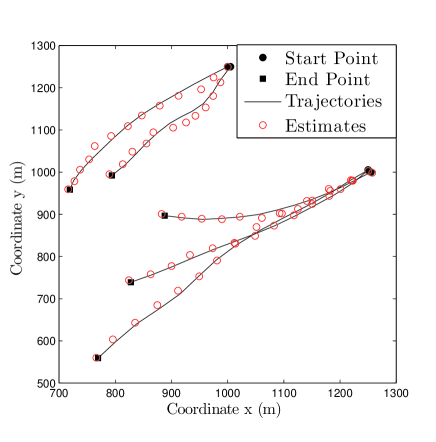
Fig. 1: Separable likelihood scenario. Targets appear from the top right corner and move closer to the radar positioned at the Cartesian origin.

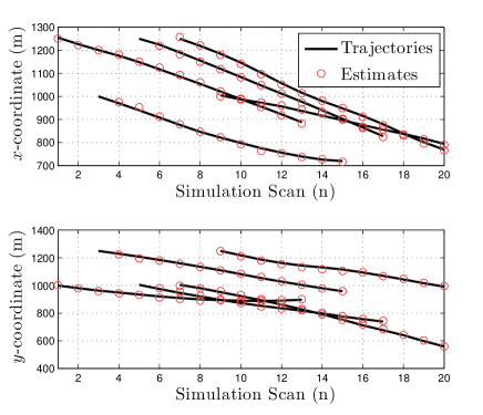
Fig. 2: Separable likelihood scenario. Estimated trajectories along the $x$ and $y$ coordinates.

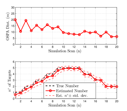
Fig. 3: Separable likelihood scenario. Monte Carlo results for estimated number of targets (top) and the OSPA distance (bottom) with cut-off $c=50\mbox{m}$

The considered scenario is depicted in Fig. 1: we have a time varying number of targets due to various births and deaths with a maximum of $5$ targets present mid scenario. The parameters are reported in Tables I and II. Fig. 2 shows the estimation results for a single trial along the $x$ and $y$ coordinates, and Fig. 3 shows the Monte Carlo results for the estimated number of targets and positional OSPA distance. Notice that the average estimated number of targets slightly differs from the true number due to closely spaced targets (see Fig. 1), but the overall performance is satisfactory given the low SNR of $7\mbox{dB}$.

V-D Non-Separable Likelihood Results

In this section we consider a more difficult radar TBD scenario where the separable likelihood assumption would lead to a bias on the estimated number of targets. Fig. 4 shows a time varying number of targets due to various births and deaths with a maximum of $7$ targets present mid scenario. Fig. 5 shows range-azimuth, range-Doppler, and azimuth-Doppler maps of the received power returns. Notice that for each 2D map, the index of the $3{}^{rd}$ coordinate is such that all maps refer to the same group of targets. Specifically, the target reflection around ($1500$m, $0.8^{\circ}$, $18$m/s) is due to two targets in the same Radar cell. This leads to the so-called unresolved target problem, which usually results in track loss when using a standard detection based approach or a separable likelihood assumption. The parameters used in simulation are reported in Tables I and III.

Table III: Non-Separable Likelihood Parameters

Parameter	Symbol	Value
Range Resolution	$R$	$20\mbox{m}$
Azimuth Resolution	$B$	$2{}^{\circ}$
Doppler Resolution	$D$	$2\mbox{m}/\mbox{s}$
Sampling Time	$T_{s}$	$1\mbox{s}$
Birth Covariance	$Q_{B}$	$\mbox{diag}\left([400,100,400,100]\right)$

The estimation results for a single trial along the $x$ and $y$ coordinates are shown in Fig. 6, and the Monte Carlo results for the estimated number of targets and positional OSPA error is shown in Fig. 7. The results demonstrate that the proposed GLMB approximation exhibits satisfactory tracking performance.

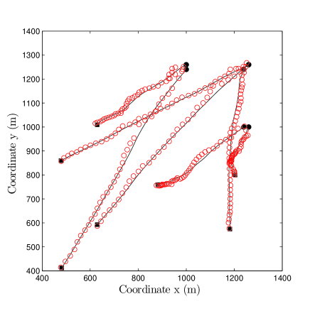
Fig. 4: Non-separable likelihood scenario. Targets appear from the top right corner and move closer to the radar positioned at the Cartesian origin.

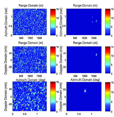
Fig. 5: Non-separable likelihood scenario. Range-Azimuth, Range-Doppler, and Azimuth-Doppler maps at time instant $k=19$. Ideal or noiseless measurement (right column), and noisy measurement (left column). Notice that for each 2D map, the index of the $3{}^{rd}$ coordinate is such that all maps refer to the same group of targets. Specifically, the target reflection around ($1500$m,$0.8^{\circ}$,$18$m/s) is due to two targets in the same Radar cell.

VI Conclusions

This paper has proposed a tractable class of GLMB approximations for labeled RFS densities. In particular, we derived from this class of GLMBs an approximation that can capture the statistical dependence between targets, preserves the cardinality distribution and the PHD, as well as minimizes the Kullback-Leibler divergence. The result has particular significance in multi-target tracking since it leads to tractable recursive filter implementations with formal track estimates for a wide range of non-standard measurement models. A radar based TBD example with low SNR and a time varying number of closely spaced targets was presented to verify the theoretical result. The key result presented in Section III is not only important to recursive multi-target filtering but is also generally applicable to statistical estimation problems involving point processes or random finite sets.

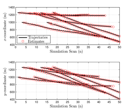
Fig. 6: Non-separable likelihood scenario.Estimated trajectories along the $x$ and $y$ coordinates.

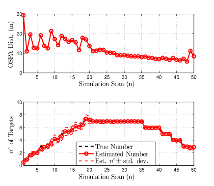
Fig. 7: Non-separable likelihood scenario. Monte Carlo results for estimated number of targets (top) and the OSPA distance (bottom) with cut-off $c=50\mbox{m}$.

References

- [1] N. Cressie, Statistics for Spatial Data. John Wiley & Sons, 1993.
- [2] P. Diggle, Statistical Analysis of Spatial Point Patterns, 2nd edition. Arnold Publishers, 2003.
- [3] R. Mahler, Statistical Multisource-Multitarget Information Fusion. Artech House, 2007.
- [4] ——, Advances in Statistical Multisource-Multitarget Information Fusion. Artech House, 2014.
- [5] K. Dralle and M. Rudemo, “Automatic estimation of individual tree positions from aerial photos,” Can. J. Forest Res, vol. 27, pp. 1728–1736, 1997.
- [6] J. Lund and M. Rudemo, “Models for point processes observed with noise,” Biometrika, vol. 87, no. 2, pp. 235–249, 2000.
- [7] J. Moller and R. Waagepeterson, “Modern Statistics for Spatial Point Processes,” Scandinavian Journal of Statistics, vol. 34, pp. 643–684, 2006.
- [8] L. Waller and C. Gotway, Applied Spatial Statistics for Public Health Data. John Wiley & Sons, 2004.
- [9] F. Baccelli, M. Klein, M. Lebourges, and S. Zuyev, “Stochastic geometry and architecture of communication networks,” Telecommunication Systems, vol. 7, no. 1-3, pp. 209–227, 1997.
- [10] M. Haenggi, “On distances in uniformly random networks,” IEEE Trans. Inf. Theory, vol. 51, no. 10, pp. 3584–3586, 2005.
- [11] M. Haenggi, J. Andrews, F. Baccelli, O. Dousse, and M. Franceschetti, “Stochastic geometry and random graphs for the analysis and design of wireless networks,” IEEE J. Sel. Areas Commun., vol. 27, no. 7, pp. 1029–1046, 2009.
- [12] S. Blackman and R. Popoli, Design and Analysis of Modern Tracking Systems. Artech House, 1999.
- [13] S. Blackman, “Multiple hypothesis tracking for multiple target tracking,” IEEE Trans. Aerosp. Electron. Syst., vol. 19, no. 1, pp. 5–18, Jan 2004.
- [14] Y. Bar-Shalom and T. Fortmann, Tracking and Data Association. Academic Press, 1988.
- [15] A. Baddeley and M. van Lieshout, Computational Statistics. Heidelberg: Physica/Springer, 1992, vol. 2, ch. ICM for object recognition, pp. 271–286.
- [16] E. Maggio, M. Taj, and A. Cavallaro, “Efficient multitarget visual tracking using random finite sets,” IEEE Trans. Circuits Syst. Video Technol., vol. 18, no. 8, pp. 1016–1027, 2008.
- [17] R. Hoseinnezhad, B.-N. Vo, D. Suter, and B.-T. Vo, “Visual tracking of numerous targets via multi-Bernoulli filtering of image data,” Pattern Recognition, vol. 45, no. 10, pp. 3625–3635, 2012.
- [18] R. Hoseinnezhad, B.-N. Vo, and B.-T. Vo, “Visual Tracking in Background Subtracted Image Sequences via Multi-Bernoulli Filtering,” IEEE Trans. Signal Process., vol. 61, no. 2, pp. 392–397, 2013.
- [19] J. Mullane, B.-N. Vo, M. Adams, and B.-T. Vo, “A Random Finite Set Approach to Bayesian SLAM,” IEEE Trans. Robot., vol. 27, no. 2, pp. 268–282, 2011.
- [20] C. Lundquist, L. Hammarstrand, and F. Gustafsson, “Road Intensity Based Mapping using Radar Measurements with a Probability Hypothesis Density Filter,” IEEE Trans. Signal Process., vol. 59, no. 4, pp. 1397–1408, 2011.
- [21] C. Lee, D. Clark, and J. Salvi, “SLAM with dynamic targets via single-cluster PHD filtering,” IEEE J. Sel. Topics Signal Process., vol. 7, no. 3, pp. 543–552., 2013.
- [22] M. Adams, B.-N. Vo, R. Mahler, and J. Mullane, “SLAM Gets a PHD: New Concepts in Map Estimation,” in IEEE Robot. Autom. Mag, 2014, pp. 26–37.
- [23] G. Battistelli, L. Chisci, S. Morrocchi, F. Papi, A. Benavoli, A. Di Lallo, A. Farina, and A. Graziano, “Traffic intensity estimation via PHD filtering,” in European Radar Conference, 2008, pp. 340–343.
- [24] D. Meissner, S. Reuter, and K. Dietmayer, “Road user tracking at intersections using a multiple-model PHD filter,” in Intelligent Vehicles Symposium (IV), 2013 IEEE, 2013, pp. 377–382.
- [25] X. Zhang, “Adaptive Control and Reconfiguration of Mobile Wireless Sensor Networks for Dynamic Multi-Target Tracking,” IEEE Trans. Autom. Control, vol. 56, no. 10, pp. 2429–2444, 2011.
- [26] J. Lee and K. Yao, “Initialization of multi-Bernoulli Random Finite Sets over a sensor tree,” in Int. Conf. Acoustics, Speech & Signal Processing (ICASSP), 2012, pp. 25–30.
- [27] G. Battistelli, L. Chisci, C. Fantacci, A. Farina, and A. Graziano, “Consensus CPHD Filter for Distributed Multitarget Tracking,” IEEE J. Sel. Topics Signal Process., vol. 7, no. 3, pp. 508–520, 2013.
- [28] M. Uney, D. Clark, and S. Julier, “Distributed Fusion of PHD Filters Via Exponential Mixture Densities,” IEEE J. Sel. Topics Signal Process., vol. 7, no. 3, pp. 521–531, 2013.
- [29] B. D. Ripley and F. P. Kelly, “Markov Point Processes,” Journal of the London Mathematical Society, vol. 2, no. 1, pp. 188–192, 1977.
- [30] M. N. M. Van Lieshout, Markov point processes and their applications. London: Imperial College Press, 2000.
- [31] O. Macchi, “The coincidence approach to stochastic point processes,” Advances in Applied Probability, vol. 7, pp. 83–122, 1975.
- [32] A. Soshnikov, “Determinantal random point fields,” Russian Mathematical Surveys, vol. 55, pp. 923–975, 2000.
- [33] J. B. Hough, M. Krishnapur, Y. Peres, and B. Virág, Zeros of Gaussian analytic functions and determinantal point processes. University Lecture Series 51. Providence, RI: American Mathematical Society, 2009.
- [34] R. Mahler, “Multi-target Bayes filtering via first-order multi-target moments,” IEEE Trans. Aerosp. Electron. Syst., vol. 39, no. 4, pp. 1152–1178, 2003.
- [35] ——, “PHD filters of higher order in target number,” IEEE Trans. Aerosp. Electron. Syst., vol. 43(3), pp. 1523–1543, July 2007.
- [36] B.-T. Vo, B.-N. Vo, and A. Cantoni, “The Cardinality Balanced Multi-target Multi-Bernoulli filter and its implementations,” IEEE Trans. Sig. Proc., vol. 57, no. 2, pp. 409–423, 2009.
- [37] D. Reid, “An algorithm for tracking multiple targets,” IEEE Trans. Autom. Control, vol. 24, no. 6, pp. 843–854, 1979.
- [38] T. Kurien, “Issues in the design of practical multitarget tracking algorithms,” in Multitarget-Multisensor Tracking: Advanced Applications, Y. Bar-Shalom, Ed. Artech House, 1990, ch. 3, pp. 43–83.
- [39] B.-T. Vo and B.-N. Vo, “Labeled Random Finite Sets and Multi-Object Conjugate Priors,” IEEE Trans. Sig. Proc., vol. 61, no. 13, pp. 3460–3475, 2013.
- [40] B.-N. Vo, B.-T. Vo, and D. Phung, “Labeled Random Finite Sets and the Bayes Multi-Target Tracking Filter,” IEEE Trans. Sig. Proc., vol. 62, no. 24, pp. 6554–6567, 2014.
- [41] Y. Boers and J. Driessen, “Particle Filter based Detection for Tracking,” in Proc. American Control Conference, 2001, pp. 4393–4397.
- [42] D. Salmond and H. Birch, “A particle filter for track-before-detect,” in Proc. American Control Conference, 2001, pp. 3755–3760.
- [43] B. Ristic, M. Arulampalam, and N. Gordon, “Detection and Tracking of Stealthy Targets,” in Beyond the Kalman Filter: Particle Filters for Tracking Applications. Artech House, 2004, ch. 11, pp. 239–259.
- [44] S. Davey, M. Rutten, and N. Gordon, “Track-Before-Detect Techniques,” in Integrated Tracking, Classification, and Sensor Management: Theory and Applications, M. Mallick, V. Krishnamurty, and B.-N. Vo, Eds. Wiley/IEEE, 2012, ch. 8, pp. 311–361.
- [45] M. Bocquel, F. Papi, M. Podt, and Y. Driessen, “Multitarget Tracking With Multiscan Knowledge Exploitation Using Sequential MCMC Sampling,” IEEE J. Sel. Topics Signal Process, vol. 7, no. 3, pp. 532–542, 2013.
- [46] F. Papi, B.-T. Vo, M. Bocquel, and B.-N. Vo, “Multi-target Track-Before-Detect using labeled random finite set,” in Control, Automation and Information Sciences (ICCAIS), 2013 International Conference on, Nov 2013, pp. 116–121.
- [47] S. Nannuru, M. Coates, and R. Mahler, “Computationally-Tractable Approximate PHD and CPHD Filters for Superpositional Sensors,” IEEE J. Sel. Topics Signal Process., vol. 7, no. 3, pp. 410–420, June 2013.
- [48] R. Mahler and A. El-Fallah, “An approximate CPHD filter for superpositional sensors,” in Proc. SPIE, vol. 8392, 2012, pp. 83 920K–83 920K–11.
- [49] M. Beard, B.-T. Vo, and B.-N. Vo, “Bayesian Multi-target Tracking with Merged Measurements Using Labelled Random Finite Sets,” IEEE Trans. Signal Process., vol. 63, no. 6, pp. 1433 – 1447, 2015.
- [50] B.-N. Vo, B.-T. Vo, N. Pham, and D. Suter, “Joint Detection and Estimation of Multiple Objects From Image Observations,” IEEE Trans. Signal Process., vol. 58, no. 10, pp. 5129–5241, 2010.
- [51] I. Goodman, R. Mahler, and H. Nguyen, Mathematics of Data Fusion. Kluwer Academic Publishers, 1997.
- [52] B.-N. Vo, S. Singh, and A. Doucet, “Sequential Monte Carlo methods for Multi-target filtering with Random Finite Sets,” IEEE Trans. Aerosp. Electron. Syst., vol. 41, no. 4, pp. 1224–1245, 2005.
- [53] S. Reuter, B.-T. Vo, B.-N. Vo, and K. Dietmayer, “The labelled multi-Bernoulli filter,” IEEE Trans. Signal Process., vol. 62, no. 12, pp. 3246–3260, 2014.
- [54] B.-N. Vo, B.-T. Vo, S. Reuter, Q. Lam, and K. Dietmayer, “Towards large scale multi-target tracking,” in SPIE Defense+ Security, vol. 9085, 2014, pp. 90 850W–90 850W–12.
- [55] R. Georgescu, S. Schoenecker, and P. Willett, “GM-CPHD and MLPDA applied to the SEABAR07 and TNO-blind multi-static sonar data,” in Information Fusion (FUSION), 2009 12th International Conference on. IEEE, 2009.
- [56] D. Svensson, J. Wintenby, and L. Svensson, “Performance evaluation of MHT and GM-CPHD in a ground target tracking scenario,” in Information Fusion (FUSION), 2009 12th International Conference on. IEEE, 2009.
- [57] J. Cardoso, “Dependence, correlation and Gaussianity in independent component analysis,” J. Mach. Learn. Res., vol. 4, pp. 1177–1203, 2003.
- [58] A. Doucet, S. J. Godsill, and C. Andrieu, “On sequential monte carlo sampling methods for bayesian filtering,” Stat. Comp., vol. 10, pp. 197–208, 2000.
- [59] T. Vu, B.-N. Vo, and R. J. Evans, “A Particle Marginal Metropolis-Hastings Multi-target Tracker,” IEEE Trans. Signal Process., vol. 62, no. 15, pp. 3953 – 3964, 2014.
- [60] F. Papi, M. Bocquel, M. Podt, and Y. Boers, “Fixed-Lag Smoothing for Bayes Optimal Knowledge Exploitation in Target Tracking,” IEEE Trans. Signal Process., vol. 62, no. 12, pp. 3143–3152, 2014.
- [61] Y. Bar-Shalom, P. K. Willett, and X. Tian, Tracking and Data Fusion: A Handbook of Algorithms. YBS Publishing, 2011.
- [62] M. Mallick, V. Krishnamurthy, and B.-N. Vo, Integrated Tracking, Classification, and Sensor Management: Theory and Applications. Wiley/IEEE, 2012.
- [63] N. Gordon, D. Salmond, and A. Smith, “Novel approach to nonlinear/non-Gaussian Bayesian state estimation ,” IEE Proceedings F on Radar and Signal Processing, vol. 140, no. 2, pp. 107–113, 1993.
- [64] B. Brewster Geelen, “Accurate solution for the modified Bessel function of the first kind,” Advances in Engineering Software, vol. 23, no. 2, pp. 105–109, 1995.