Biased Tracers and Time Evolution

Abstract

We study the effect of time evolution on galaxy bias. We argue that at any order in perturbations, the galaxy density contrast can be expressed in terms of a finite set of locally measurable operators made of spatial and temporal derivatives of the Newtonian potential. This is checked in an explicit third order calculation. There is a systematic way to derive a basis for these operators. This basis spans a larger space than the expansion in gravitational and velocity potentials usually employed, although new operators only appear at fourth order. The basis is argued to be closed under renormalization. Most of the arguments also apply to the structure of the counter-terms in the effective theory of large-scale structure.

1 Introduction

The purpose of the theory of bias is to relate observable properties of tracers such as the density contrast of galaxies $\delta_{g}$ to the underlying matter distribution and the initial conditions. If one neglects primordial non-Gaussianity and possible entropic perturbations, as we will do throughout for simplicity, then $\delta_{g}$ can only be a function of local observables of the dark-matter field (such as density, tidal forces, etc.) along the tracer’s trajectory. In the same approximation the deviation of the tracer’s trajectory from that of the underlying cosmic fluid, typically phrased as velocity bias, should also depend only on those locally observable quantities.

A standard approach in the field has been to try to write the most general functional dependence of this sort at the final time [1, 2] (Eulerian biasing). The ignorance about the underlying physics is then parameterized into a set of bias coefficients which become less and less relevant (in a perturbation theory sense) as we go to higher and higher orders in matter fluctuations and derivatives. An alternative approach is to perform the parametrization on the initial slice [3, 4, 5] (Lagrangian biasing). However, the sufficiency of either of these approaches is not totally obvious: It is true that because of deterministic evolution the full formation history can be reconstructed from the information on either the final or the initial time slice. However, because of the long-range gravitational interactions, one may suspect that the Eulerian (Lagrangian) description of galaxy distribution for a population of finite age might be non-local. Regardless of this issue, a complete and non-redundant classification of locally observable operators does not seem to exist so far.

Finally in [6] it was argued that the most general relation between tracers and the underlying matter distribution should be written as an integral over time along the fluid trajectory of all possible local observables including the tidal tensor, gradients of the velocity field and other operators with higher spatial derivatives. The relation is thus local in space but non-local in time. In [6] it was shown that the time-non-locality can be dealt with in perturbation theory.

The goal of this paper is to investigate systematically the implications of the finite age and time evolution of tracers on the effective bias parametrization. In particular we will show that all the approaches described above are mathematically equivalent and provide a dictionary between them. We will give a complete and yet non-redundant basis of operators that can be used to express the most general relation between biased tracers and the underlying matter fluctuations. We are not the first who study this problem. Considerable insight has been obtained starting from the work of Tegmark and Peebles [7]. In particular generation of nonlinear bias due to time evolution was first discussed in [8]. Evidence from numerical simulations as well as phenomenological explanations have been provided in [9, 10].

2 A Green’s function for galaxy formation

In order to study this problem, we consider instantaneous formation of tracers at time $\tau_{*}$ and write the most general expression for $\delta_{g}(\tau_{*})$ in terms of local observables, $\{O(\tau_{*})\}$, made of the underlying matter distribution with coefficients $\{b_{O}^{*}\}$:

$$\delta_{g}(\mathbf{x},\tau_{*})=\sum_{O}b_{O}^{*}O(\mathbf{x},\tau_{*})\,.$$ (2.1)

Postulating the conservation of the tracers we then solve for $\delta_{g}(\tau)$ at later times. We shall see that this provides a Green’s function for galaxy biasing. Any formation history which depends on locally measurable quantities can be obtained by a superposition of these conserved tracers. A similar approach was used in [6].

One should ask what are the locally measurable quantities that instantaneously forming objects can depend upon. As long as the tracers are well described as a non-relativistic fluid, the gravitational effects are fully captured by the potential $\phi$ (i.e. the perturbation to the time-time component of the metric), which for convenience is rescaled to $\Phi\equiv 2\phi/3\mathcal{H}^{2}\Omega_{m}$, satisfying $\nabla^{2}\Phi=\delta$. Because of the equivalence principle, only tidal forces made of various powers of $\partial_{i}\partial_{j}\Phi$ are measurable; a uniform, but possibly time-dependent, gravitational force $\partial_{i}\Phi(t)$ causes a uniform acceleration of all objects and hence cannot be seen by any local measurement. It follows that locally measurable quantities have to be invariant under time-dependent but uniform translations.

In addition to $\partial_{i}\partial_{j}\Phi$, its spatial derivatives as well as time derivatives along the flow of dark matter are also locally measurable. Throughout, we always work with this convective time derivative defined through

$$\frac{\rm D}{\rm d\tau}O(\mathbf{x},\tau)\equiv\left[\partial_{\tau}+\mathbf{v}\cdot\partial_{x}\right]O(\mathbf{x},\tau)\,,$$ (2.2)

where $\mathbf{v}(\mathbf{x},\tau)$ is the matter peculiar velocity field.

Since $\partial_{i}\partial_{j}\Phi$ is dimensionless, additional derivatives must be accompanied by the characteristic size and formation time scale of the object which are denoted respectively by $L$ and $T$. The scale $L$ is naively expected to be that which encloses the mass of the object at the background density, i.e. the Lagrangian radius of the object, although baryonic feedback and radiative transfer effects could in principle increase this scale for certain tracers. The time scale $T$ on the other hand is expected to be typically the Hubble time $T\sim\mathcal{H}^{-1}(\tau_{*})$, the same scale that is used to define $\Phi$. Higher order spatial derivatives associated with the length scale $L$ are not directly relevant for the issue of time evolution which we are concerned with here. Thus, throughout the paper we will only consider terms that are lowest order in spatial derivatives. This means that each instance of $\Phi$ will come with exactly two spatial derivatives.

We are therefore interested in the evolution of local observables along the large-scale flow of dark-matter. (We assume zero velocity bias for the moment. It is considered later and shown to be higher order in spatial derivatives.) This problem is naturally posed in the Lagrangian formalism where fluid trajectories are labeled by their initial position $\mathbf{q}$ and are implicitly defined by

$$\mathbf{x}_{\rm fl}(\mathbf{q},\tau)=\mathbf{q}+\mathbf{s}(\mathbf{q},\tau)\,,$$ (2.3)

where $\mathbf{s}(\mathbf{q},0)=0$. The displacement then satisfies

$$\mathbf{s}(\mathbf{q},\tau_{0})=\int_{0}^{\tau_{0}}\mathbf{v}(\mathbf{x}_{\rm fl}(\mathbf{q},\tau),\tau){\rm d}\tau\,.$$ (2.4)

We will frequently drop the $\mathbf{q}$ argument in $\mathbf{x}_{\rm fl}$ when there is no ambiguity.

The system to solve for $\tau>\tau_{*}$ consists of the continuity equations for tracer and matter in addition to the Euler equation,

$$\frac{{\rm D}}{{\rm d}\tau}\delta =\> -\theta(1+\delta),$$ (2.5)

$$\frac{{\rm D}}{{\rm d}\tau}\theta =\> -\mathcal{H}\theta-\frac{3}{2}\Omega_{m}\mathcal{H}^{2}\delta-(\partial_{x}^{i}\mathbf{v}^{j})^{2}\,,$$ (2.6)

$$\frac{{\rm D}}{{\rm d}\tau}\delta_{g} =\> -\theta(1+\delta_{g})$$ (2.7)

where ${\rm D}/{\rm d}\tau$ is the convective derivative and $\theta=\partial_{x}^{i}v_{i}$ is the dark matter velocity divergence.

2.1 Flow of dark matter

The first two equations are independent of the last one and describe the time evolution of dark matter. In the standard perturbation theory $\delta(\mathbf{x},\tau)$ and $\theta(\mathbf{x},\tau)$ are solved in powers of the initial field $\delta_{1}(\mathbf{x})$ evaluated at the same position $\mathbf{x}$. For instance, $\delta^{[1]}(\mathbf{x},\tau)=D(\tau)\delta_{1}(\mathbf{x})$ and

$$\delta^{[2]}(\mathbf{x},\tau)=D^{2}(\tau)\left[\frac{5}{7}\delta_{1}^{2}(\mathbf{x})+\frac{2}{7}\left(\frac{\partial_{i}\partial_{j}}{\nabla^{2}}\delta_{1}(\mathbf{x})\right)^{2}+\left(\frac{\partial_{i}}{\nabla^{2}}\delta_{1}(\mathbf{x})\right)\partial_{i}\delta_{1}(\mathbf{x})\right],$$ (2.8)

where $D(\tau)$ is the linear growth factor normalized to $a(\tau)$ during matter domination. We have made the usual very accurate approximation of replacing the $n$-th order growth factor with $D^{n}(\tau)$.

The last term in the above expression for $\delta^{[2]}$ blows up in the presence of an infinitely long-wavelength mode. The leading effect of the long wavelength mode is a large uniform acceleration, and the last term of Eq. (2.8) is the displacement needed to move the argument of the linear solution from $\mathbf{x}$ to the initial Lagrangian position: $\delta_{1}(\mathbf{x})=\delta_{1}(\mathbf{q})-D(\tau)(\partial_{i}/\nabla^{2})\delta_{1}(\mathbf{x})\partial_{i}\delta_{1}(\mathbf{x})+\mathcal{O}(\delta_{1}^{3})$. Similarly, the third order solution $\delta^{[3]}(\mathbf{x},\tau)$ is shown in appendix App. C to contain terms which diverge in the presence of infinite wavelength modes. They are needed to displace lower order solutions from $\mathbf{x}$ to $\mathbf{q}$. Therefore, expanding $\delta(\mathbf{x},\tau)$ in terms of the initial field at the Lagrangian position $\delta_{1}(\mathbf{q})$ yields

$$\delta(\mathbf{x},\tau)=D(\tau)\delta_{\rm lgr}^{[1]}(\mathbf{q})+D^{2}(\tau)\delta_{\rm lgr}^{[2]}(\mathbf{q})+D^{3}(\tau)\delta_{\rm lgr}^{[3]}(\mathbf{q})+\cdots$$ (2.9)

where now $\delta_{\rm lgr}^{[2]}(\mathbf{q})=5/7\delta_{1}^{2}(\mathbf{q})+2/7[(\partial_{i}\partial_{j}/\nabla^{2})\delta_{1}(\mathbf{q})]^{2}$ and $\delta_{\rm lgr}^{[3]}(\mathbf{q})$, given below, are Lagrangian operators constructed from the initial density field $\delta_{\rm lgr}^{[1]}(\mathbf{q})=\delta_{1}(\mathbf{q})$. They remain finite in the presence of long wavelength modes. In fact, the structure of Eq. (2.5) and Eq. (2.6) ensures that this holds to all orders, since (a) after expressing $\delta$ and $\theta$ as a function of $(\mathbf{q},\tau)$ the convective derivative reduces to an ordinary time derivative, and then (b) every term in the equation can be written in terms of $\partial_{i}\partial_{j}\Phi$ or $\partial_{i}v_{j}$, which remain finite for infinitely long-wavelength perturbations. In App. B and independently in Sec. 3 we provide methods of solving directly for $\delta_{\rm lgr}^{[n]}(\mathbf{q})$.

What we mean by an $n^{th}$ order Lagrangian operator is that in momentum space there is no singularity when any subset of $n$ momenta $\{\mathbf{k}_{a}\}$ is taken to zero, with $\{\delta_{1}(\mathbf{k}_{a})\}$ kept fixed. This doesn’t ensure that the operator has a spatially local expression [even in terms of $\Phi_{1}(\mathbf{q})\equiv\nabla^{-2}\delta_{1}(\mathbf{q})$], as can be seen from the explicit solution

$$\delta_{\rm lgr}^{[3]}(\mathbf{q})=\>\frac{341}{567}\delta_{1}^{3}+\frac{11}{21}\delta_{1}K_{1}^{2}+\frac{2}{9}K_{1}^{3}+\frac{4}{63}K_{1}^{ij}\mathcal{D}_{ij}\left[\delta_{1}^{2}-\frac{3}{2}K_{1}^{2}\right]\,,$$ (2.10)

where the derivative operator $\mathcal{D}_{ij}$ and the traceless tidal tensor are defined respectively as

$$\mathcal{D}_{ij}\equiv\left(\frac{\partial_{i}\partial_{j}}{\nabla^{2}}-\frac{1}{3}\delta_{ij}\right);\quad K^{1}_{ij}(\mathbf{q})\equiv\mathcal{D}_{ij}\delta_{1}(\mathbf{q})\,.$$ (2.11)

The term in Eq. (2.10) involving $\mathcal{D}_{ij}(\delta_{1}^{2}-3K_{1}^{2}/2)$ cannot be written as a local combination of $\partial_{i}\partial_{j}\Phi_{1}$. Since this is an important distinction for the discussion in this paper, let us emphasize again: locally measurable observables contain spatially nonlocal Lagrangian operators in their expansion.

Beyond the density $\delta(\mathbf{x},\tau)$, the equivalence principle ensures that any locally measurable quantity, including the tidal tensor $\partial_{i}\partial_{j}\Phi(\mathbf{x},\tau)$, can be solved along the flow in terms of such Lagrangian operators. Hence for any scalar $O$ involving $d_{O}$ powers of $\partial_{i}\partial_{j}\Phi$ we have:

$$O(\mathbf{x},\tau)=D^{d_{O}}(\tau)O_{\rm lgr}^{[d_{O}]}(\mathbf{q})+D^{d_{O}+1}(\tau)O_{\rm lgr}^{[d_{O}+1]}(\mathbf{q})+\cdots$$ (2.12)

where the first component $O_{\rm lgr}^{[d_{O}]}(\mathbf{q})$ is the same as $O(\mathbf{x},\tau)$ with the replacement

$$\partial_{i}\partial_{j}\Phi(\mathbf{x},\tau)\to(\partial_{i}\partial_{j}\Phi)_{\rm lgr}^{[1]}(\mathbf{q})\equiv\frac{\partial_{i}\partial_{j}}{\nabla^{2}}\delta_{1}(\mathbf{q}).$$ (2.13)

Higher order $O_{\rm lgr}^{[n]}(\mathbf{q})$ are constructed from products of $d_{O}$ factors of $(\partial_{i}\partial_{j}\Phi)_{\rm lgr}^{[m_{a}]}(\mathbf{q})$ with $\sum_{a=1}^{d_{O}}m_{a}=n$.

2.2 Flow of galaxies

Let us now turn to Eq. (2.7) to solve for $\delta_{g}(\tau)$. It is useful to subtract Eq. (2.5) to get

$$\frac{{\rm D}}{{\rm d}\tau}\ (\delta_{g}-\delta)=-\theta(\delta_{g}-\delta).$$ (2.14)

This is a linear and homogeneous equation in $\delta_{g}-\delta$, hence we can make use of the superposition principle. The solution $\delta_{g}(\tau)$ for an arbitrary formation history can be obtained by breaking the formation into instantaneous events and superposing the corresponding solutions.

We now show that if $\delta_{g}(\tau_{*})$ has a bias expansion fully in terms of local operators as in Eq. (2.1), then at any later time it remains local:

$$\delta_{g}(\mathbf{x},\tau)=\sum_{O}b_{O}(\tau)O(\mathbf{x},\tau)\,,$$ (2.15)

where the sum is over all local operators, and $\{b_{O}(\tau)\}$ are uniquely determined in terms of $\{b_{O}^{*}\}$. We proceed now with the general derivation; an explicit calculation showing how this works in practice up to third order will appear below in Sec. 2.3.

Substituting Eq. (2.15) as an ansatz for $\delta_{g}(\tau)$ and Eq. (2.12) for operators in Eq. (2.14), and using the fact that convective derivative becomes an ordinary derivative when acted on functions of $(\mathbf{q},\tau)$, we obtain

$$\sum_{O}\sum_{n=d_{O}}^{\infty}\left[\frac{{\rm d}\tilde{b}_{O}}{{\rm d}\tau}+\tilde{b}_{O}\left(n\frac{{\rm d}\log D(\tau)}{{\rm d}\tau}+\sum_{m=1}^{\infty}D^{m}(\tau)\theta_{\rm lgr}^{[m]}(\mathbf{q})\right)\right]D^{n}(\tau)O_{\rm lgr}^{[n]}(\mathbf{q})=0,$$ (2.16)

where $\tilde{b}_{O}\equiv b_{O}$ except for $\tilde{b}_{\delta}\equiv b_{1}-1$. There is a lot of overlap among $O_{\rm lgr}^{[n]}(\mathbf{q})$ and their products for various $O(\mathbf{x},\tau)$ operators. Expressing everything in Eq. (2.16) in terms of a linearly independent basis for Lagrangian operators $\{E_{\rm lgr}(\mathbf{q})\}$, and setting the coefficient of each one to zero yields a set of coupled first order ODE’s for the bias parameters $\{b_{O}(\tau)\}$, with the initial condition $b_{O}(\tau_{*})=b_{O}^{*}$.

Let us also expand local operators $\{O(\mathbf{x},\tau)\}$ in terms of a linearly independent Eulerian basis $\{\hat{E}(\mathbf{x},\tau)\}$, and introduce a bias parameter $b_{\hat{E}}(\tau)$ for each. The system is guaranteed to have a solution if every $E_{\rm lgr}(\mathbf{q})$ can be mapped to a unique local operator $\hat{E}(\mathbf{x},\tau)$ such that ${\rm d}\tilde{b}_{\hat{E}}/{\rm d}\tau$ multiplies $E_{\rm lgr}(\mathbf{q})$ in Eq. (2.16). At first sight this may seem not to be possible. Naively, there seems to be many $O_{\rm lgr}^{[n]}(\mathbf{q})$ for every $O(\mathbf{x},\tau)$ and as we saw in Eq. (2.10) they often have spatially non-local structures. This structure will appear in one of the $E_{\rm lgr}(\mathbf{q})$ and if there is no analogous locally measurable operator, the ansatz (2.15) would fail.

However, the non-local structures that appear in $O^{[n]}_{\rm lgr}(\mathbf{q})$ are not arbitrary. And indeed we can show that every $O_{\rm lgr}^{[n]}(\mathbf{q})$ can be mapped to a local Eulerian operator $\hat{O}^{[n]}(\mathbf{x},\tau)$ which is unique up to the addition of higher order local operators. Recall that the convective derivative of a locally measurable quantity is also locally measurable. Since in the expansion Eq. (2.12) every $O_{\rm lgr}^{[n]}$ is accompanied by a different power of $D(\tau)$, by combining convective time derivatives of $O(\mathbf{x},\tau)$ we can easily construct the desired operator

$$\hat{O}^{[n]}(\mathbf{x},\tau)=D^{n}(\tau)O_{\rm lgr}^{[n]}(\mathbf{q})+\mathcal{O}(\delta^{n+1}).$$ (2.17)

For instance, $\hat{O}^{[d_{O}]}(\mathbf{x},\tau)\equiv O(\mathbf{x},\tau)$, and at next order:

$$\hat{O}^{[d_{O}+1]}(\mathbf{x},\tau)\equiv O^{\prime}(\mathbf{x},\tau)-d_{O}O(\mathbf{x},\tau),$$ (2.18)

where prime denotes convective derivative with respect to $\log D(\tau)$:

$$O^{\prime}(\mathbf{x},\tau)=\frac{{\rm D}}{{\rm d}\log D(\tau)}O(\mathbf{x},\tau)=\frac{D(\tau)}{\dot{D}(\tau)}\frac{{\rm D}}{{\rm d}\tau}O(\mathbf{x},\tau).$$ (2.19)

At higher orders $\hat{O}^{[n]}(\mathbf{x},\tau)$ can be constructed recursively:

$$\hat{O}^{[n]}\equiv\frac{1}{(n-d_{O})!}\left[(\hat{O}^{[n-1]})^{\prime}-(n-1)\hat{O}^{[n-1]}\right].$$ (2.20)

The above mapping leads to a one to one mapping between the linearly independent bases of operators $\{E_{\rm lgr}(\mathbf{q})\}$ and $\{\hat{E}(\mathbf{x},\tau)\}$, and confirms the sufficiency of the ansatz Eq. (2.15).

To lowest order in spatial derivatives, a complete and non-redundant basis $\{E_{\rm lgr}(\mathbf{q})\}$ for all $\{O_{\rm lgr}^{[n]}\}$, is made of all scalars that can be constructed from products of $\Pi^{[n]}_{ij}(\mathbf{q})\equiv(\partial_{i}\partial_{j}\Phi)_{\rm lgr}^{[n]}(\mathbf{q})$. By the equations of motion ${\rm Tr}[\Pi_{ij}^{[n]}]$ can be expressed in terms of lower order traces and hence is not independent. We therefore have up to fourth order (and using matrix notation)

$${\rm 1^{st}}\ \ {\rm Tr}[\Pi^{[1]}]$$ (2.21)

$${\rm 2^{nd}}\ \ {\rm Tr}[(\Pi^{[1]})^{2}],\ ({\rm Tr}[\Pi^{[1]}])^{2}$$

$${\rm 3^{rd}}\ \ {\rm Tr}[(\Pi^{[1]})^{3}],\ {\rm Tr}[(\Pi^{[1]})^{2}]{\rm Tr}[\Pi^{[1]}],\ ({\rm Tr}[\Pi^{[1]}])^{3},\ {\rm Tr}[\Pi^{[1]}\Pi^{[2]}]$$

$${\rm 4^{th}}\ \ {\rm Tr}[(\Pi^{[1]})^{4}],\ {\rm Tr}[(\Pi^{[1]})^{3}]{\rm Tr}[\Pi^{[1]}],\ {\rm Tr}[(\Pi^{[1]})^{2}]{\rm Tr}[(\Pi^{[1]})^{2}],\ ({\rm Tr}[\Pi^{[1]}])^{4},\ {\rm Tr}[\Pi^{[1]}\Pi^{[3]}],$$

$$\ {\rm Tr}[\Pi^{[2]}\Pi^{[2]}].$$

In practice it is more natural to work with the distortion matrix $M^{ij}=\partial_{q}^{i}s^{j}$ in the Lagrangian space. In Sec. 3 we will discuss the connection between the two sets of variables and write an identically looking basis in terms of various $M_{ij}^{[n]}(\mathbf{q})$.

To obtain the corresponding Eulerian basis $\{\hat{E}(\mathbf{x},\tau)\}$, we define the analogs of $\Pi_{ij}^{[n]}(\mathbf{q})$. The time-derivatives of $\partial_{i}\partial_{j}\Phi(\mathbf{x},\tau)$ can be combined to obtain Eulerian operators $\hat{\Pi}_{ij}^{[n]}(\mathbf{x},\tau)$ whose leading order expression in perturbation theory are given by $\hat{\Pi}_{ij}^{[n]}(\mathbf{x},\tau)=D^{n}(\tau)\Pi_{ij}^{[n]}(\mathbf{q})+\mathcal{O}(\delta^{n+1})$. Starting from

$$\hat{\Pi}^{[1]}_{ij}(\mathbf{x},\tau)=\>\partial_{i}\partial_{j}\Phi(\mathbf{x},\tau),$$ (2.22)

the higher order operators can again be calculated recursively. Suppressing the indices and the argument $(\mathbf{x},\tau)$

$$\hat{\Pi}^{[n]}=\>\frac{1}{(n-1)!}\left[(\hat{\Pi}^{[n-1]})^{\prime}-(n-1)\hat{\Pi}^{[n-1]}\right].$$ (2.23)

The Eulerian basis is then composed of all scalars constructed out of $\hat{\Pi}^{[n]}_{ij}$ excluding ${\rm Tr}[\hat{\Pi}^{[n]}]$; in other words, it can be obtained by replacing $\Pi$ with $\hat{\Pi}$ in Eq. (2.21). We conclude by a few comments:

• The tensors $\hat{\Pi}^{[n]}(\mathbf{x},\tau)$, and hence the Eulerian operators $\{\hat{E}(\mathbf{x},\tau)\}$, are easily calculable in momentum space by combining the $F$ and $G$ kernels of the Standard Perturbation Theory (SPT). For instance,

  $$\hat{\Pi}^{[1]}_{ij}(\mathbf{k},\tau)=\>\frac{\mathbf{k}^{i}\mathbf{k}^{j}}{|\mathbf{k}|^{2}}\sum_{n=1}^{\infty}D^{n}(\tau)\delta_{n}(\mathbf{k}),$$ (2.24)

  where $\delta_{n}(\mathbf{k})$ is the $n^{th}$ order SPT solution, and

  $$\begin{split}\hat{\Pi}^{[2]}_{ij}(\mathbf{k},\tau)=\>\sum_{n=1}^{\infty}D^{n}(\tau)\Big{[}&\frac{\mathbf{k}^{i}\mathbf{k}^{j}}{|\mathbf{k}|^{2}}(n-1)\delta_{n}(\mathbf{k})\\[8.0pt] &+\sum_{m=1}^{n-1}\int\frac{{\rm d}^{3}\mathbf{p}}{(2\pi)^{3}}\frac{(\mathbf{k}-\mathbf{p})\cdot\mathbf{p}}{|\mathbf{k}-\mathbf{p}|^{2}}\frac{\mathbf{p}^{i}\mathbf{p}^{j}}{|\mathbf{p}|^{2}}\theta_{m}(\mathbf{k}-\mathbf{p})\delta_{n-m}(\mathbf{p})\Big{]},\end{split}$$ (2.25)

  and so on.

• One should bear in mind that although $\partial_{i}\partial_{j}\Phi(\mathbf{x},\tau)$ is a total derivative, neither its convective time derivatives nor the $\mathbf{q}$-space matrices $\Pi_{ij}^{[n]}(\mathbf{q})$ have necessarily to be full spatial derivatives of any kind.

• The list (2.21) spans only the subset of Lagrangian operators that appear in the expansion of local operators. There are infinitely many more Lagrangian operators. For instance, at third order one may expect at least five operators:

  $$\delta_{1}^{3},\quad\delta_{1}K_{1}^{2},\quad K_{1}^{3},\quad K_{1}^{ij}\mathcal{D}_{ij}\delta_{1}^{2},\quad K_{1}^{ij}\mathcal{D}_{ij}K_{1}^{2},$$ (2.26)

  but there are four in Eq. (2.21). The last two operators always appear with relative factor $-3/2$ in the expansion of local operators, as in Eq. (2.10).

• If $\{b_{O}^{*}\}$ were known we could obtain $\{b_{O}(\tau)\}$ by solving Eq. (2.16). Even if $b_{O}(\tau_{*})=0$ for some operator, generically it will be non-zero after time evolution. (Examples of this will be seen in the next section.) In the absence of that information, an effective Eulerian bias can be fully formulated in terms of local operators with unknown coefficients.

• Up to third order our Eulerian list consists of seven operators and agrees with [1, 8, 2]. Starting from third order convective time derivatives are needed (i.e. our $\hat{\Pi}^{[2]}(\mathbf{x},\tau)$ operator.) In terms of the commonly used velocity potential $\nabla^{2}\Phi_{v}=-\mathcal{H}^{-1}\theta$, we have

  $$\hat{\Pi}^{[2]}_{ij}=\partial_{i}\partial_{m}\Phi\partial_{j}\partial_{m}\Phi+\frac{5}{2}(\partial_{i}\partial_{j}\Phi-\partial_{i}\partial_{j}\Phi_{v})+\mathcal{O}(\delta^{3}).$$ (2.27)

  Clearly, at higher orders $\partial_{i}\partial_{j}\Phi$ and $\partial_{i}\partial_{j}\Phi_{v}$ will be insufficient for a local description of bias and higher order time derivatives will be necessary. The first example is the quartic operator ${\rm Tr}(\hat{\Pi}^{[1]}\hat{\Pi}^{[3]})$. This contributes to five-point correlation function of $\delta_{g}$ at tree level, and the power-spectrum at two loops.

2.3 Bias evolution at third order: explicit calculation

In this section, we explicitly derive the density field of tracers $\delta_{g}$ at time $\tau$ given formation at some earlier time $\tau_{*}$, up to third order in perturbation theory. This will illustrate the general time-dependence of the bias parameters, and confirms the arguments of last section. For this calculation, we use an approach we call “convective SPT”, which is a hybrid of the standard Eulerian perturbation theory (SPT) and Lagrangian perturbation theory (LPT) approaches. The details are provided in App. B.

At $\tau_{*}$, we start from the most general, local, third order expression for $\delta_{g}(\tau_{*})$ [8]:

$$\begin{split}\delta_{g}^{*}=\delta_{g}(\mathbf{x}_{\rm fl}(\tau_{*}),\tau_{*})=\>\sum_{n=1}^{3}&\frac{b_{n}^{*}}{n!}[\delta^{*}]^{n}+\sum_{n=2}^{3}\frac{b_{K^{n}}^{*}}{n!}{\rm Tr}\left[(K_{ij}^{*})^{n}\right]\\[5.0pt] &+\frac{1}{6}b^{*}_{\delta K^{2}}\delta^{*}\>{\rm Tr}\left[(K_{ij}^{*})^{2}\right]+\frac{1}{6}b^{*}_{\Gamma}\Gamma^{*}+\epsilon^{*}\,,\end{split}$$ (2.28)

where all quantities are measured at $(\mathbf{x}_{\rm fl}(\tau_{*}),\tau_{*})$. We have defined

$$K_{ij}(\mathbf{x},\tau)\equiv\> \hat{\Pi}^{[1]}_{ij}-\frac{1}{3}\delta_{ij}{\rm Tr}(\hat{\Pi}^{[1]}),$$ (2.29)

$$\Gamma(\mathbf{x},\tau)\equiv\> \frac{21}{10}K^{ij}(\hat{\Pi}^{[2]}_{ij}-\hat{\Pi}^{[1]}_{ik}\hat{\Pi}^{[1]}_{jk}).$$ (2.30)

Using the definition (2.11), the leading Lagrangian component of $\Gamma$ is

$$\Gamma^{[3]}_{\rm lgr}(\mathbf{q})=K_{1}^{ij}\mathcal{D}_{ij}\left[\delta_{1}^{2}-\frac{3}{2}K_{1}^{2}\right]$$ (2.31)

In the second line of Eq. (2.28), we have introduced a stochastic variable $\epsilon^{*}(\mathbf{x})$ (considered first order in perturbations) which is defined on the formation time slice and captures the fluctuations in galaxy density that are uncorrelated with long-wavelength perturbations. However, the statistical properties of the stochastic term in general also depend on local observables. Thus, in order to keep track of the effect of stochasticity up to cubic order in fluctuations we write:

$$\epsilon^{*}=\epsilon^{*}_{0}+\epsilon^{*}_{\delta}\delta^{*}+\frac{1}{2}\epsilon^{*}_{\delta^{2}}[\delta^{*}]^{2}+\frac{1}{2}\epsilon^{*}_{K^{2}}{\rm Tr}\left[(K_{ij}^{*})^{2}\right]+\cdots$$ (2.32)

where $\epsilon^{*}_{\alpha}$ are stochastic variables. At the order we are working in, for two-point correlation functions one needs to know $\langle\epsilon^{*}_{0}\epsilon^{*}_{0}\rangle$ and three other correlations to describe the dependence on the long wavelength modes: $\langle\epsilon^{*}_{\delta}\epsilon^{*}_{\delta}\rangle$, $\langle\epsilon^{*}_{0}\epsilon^{*}_{\delta^{2}}\rangle$ and $\langle\epsilon^{*}_{0}\epsilon^{*}_{K^{2}}\rangle$.

We solve Eq. (2.14) as described in App. B, and arrive at the following expression at later times along the fluid trajectory:

$$\delta_{g}(\mathbf{x}_{\rm fl}(\tau),\tau)=\> \sum_{n=1}^{3}\frac{b_{n}^{E}}{n!}\delta^{n}+\sum_{n=2}^{3}\frac{b_{K^{n}}^{E}}{n!}{\rm Tr}\left[K_{ij}^{n}\right]+\frac{1}{6}b_{\delta K^{2}}^{E}\delta\>{\rm Tr}\left[K_{ij}^{2}\right]+\frac{1}{6}b_{\Gamma}^{E}\Gamma$$ (2.33)

$$+\epsilon^{*}_{0}+\epsilon_{\delta}^{E}\delta+\frac{1}{2}\epsilon_{\delta^{2}}^{E}\delta^{2}+\frac{1}{2}\epsilon_{K^{2}}^{E}{\rm Tr}\left[K_{ij}^{2}\right]\,,$$

where the quantities on the r.h.s. are evaluated at $(\mathbf{x}_{\rm fl}(\tau),\tau)$. Note that as anticipated the list of local operators is sufficient to express the time-evolved $\delta_{g}(\tau)$.

The Eulerian bias coefficients $b_{O}^{E}$ are given in terms of $b^{*}_{O}$ in Eq. (B.33) and Eq. (B.38). Let us quote some of them for reference:

$$b_{1}^{E}(\tau)=\> (b_{1}^{*}-1)D_{*}+1,$$ (2.34)

$$b_{2}^{E}(\tau)=\> b_{2}^{*}D_{*}^{2}-\frac{8}{21}(b_{1}^{*}-1)D_{*}(D_{*}-1),$$ (2.35)

$$b_{K^{2}}^{E}(\tau)=\> b_{K^{2}}^{*}D_{*}^{2}+\frac{4}{7}(b_{1}^{*}-1)D_{*}(D_{*}-1),$$ (2.36)

$$b_{\Gamma}^{E}(\tau)=\> b_{\Gamma}^{*}D_{*}^{3}+\left[(b_{1}^{*}-1)\left(-\frac{8}{21}\right)\left(\frac{23}{7}-D_{*}\right)+\frac{20}{7}b_{K^{2}}^{*}D_{*}\right]D_{*}(D_{*}-1)$$ (2.37)

where $D_{*}=D(\tau_{*})/D(\tau)$. The Eulerian stochasticity terms $\epsilon^{E}_{\alpha}$ are given in Eq. (B.34) and Eq. (B.42).

In general, obtaining these bias coefficients requires a detailed calculation. However there is a subset of operators for which obtaining the time dependence of the bias parameters is rather straightforward. The key observation is that the r.h.s. of Eq. (2.14) is a product two scalar operators $\theta(\delta_{g}-\delta)$. If we substitute the bias expansion (2.15) and expand in terms of a linearly independent Lagrangian basis of operators, every operator on the r.h.s. would be factorizable, i.e. it can be written as a product of two scalars. Thus, any term in $\delta_{g}-\delta$ that cannot be written as a product of two scalar operators must be time-independent.

Suppose $O(\mathbf{x},\tau)$ is non-factorizable (for instance it can be $\delta$ or $K_{ij}^{2}$), then so is $O_{\rm lgr}^{[d_{O}]}(\mathbf{q})$. If $O_{\rm lgr}^{[d_{O}]}(\mathbf{q})$ does not appear in the Lagrangian solution for any other operator, for its coefficient to be time-independent, we must have

$$b_{O}(\tau)=b_{O}^{*}D_{*}^{d_{O}}(\tau)\qquad\text{with}\qquad D_{*}(\tau)=\frac{D(\tau_{*})}{D(\tau)}\,.$$ (2.38)

For instance consider the case where $O$ is just $\delta$. Then we conclude that $(b_{1}-1)D(\tau)\delta_{1}(\mathbf{q})$ is time independent because the r.h.s. of Eq. (2.14) starts at second order. As a result, $(b_{1}-1)\propto{D^{-1}(\tau)}$, as implied by Eq. (2.38). This agrees with Eq. (2.34). If $O^{[d_{O}]}_{\rm lgr}$ does appear in the expansion of some lower order operator $P$, then by superposition principle we can still write Eq. (2.38) plus corrections proportional to $b_{P}^{*}$. For instance, If $O=K^{2}$ then $(K^{2})^{[2]}_{\rm lgr}=K_{1}^{2}(\mathbf{q})$ also appears in the second order solution $\delta^{[2]}_{\rm lgr}(\mathbf{q})$. Therefore we have $b_{K^{2}}=b_{K^{2}}^{*}D_{*}^{2}(\tau)$ plus terms proportional to $b_{1}^{*}-1$, in agreement with Eq. (2.36).

Now consider a higher order non-factorizable operator $O_{\rm lgr}^{[n]}$ in the perturbative expansion of $O$. It is multiplied by $b_{O}(\tau)D^{n}(\tau)$ which is time-dependent. To make the entire contribution proportional to $O_{\rm lgr}^{[n]}$ time-independent and thus equal to its value at $\tau_{*}$, there needs to be an associated Eulerian operator $\hat{O}^{[n]}(\mathbf{x},\tau)=D^{n}(\tau)O_{\rm lgr}^{[n]}(\mathbf{q})+\mathcal{O}(\delta^{n+1})$ whose bias parameter satisfies

$$\frac{{\rm d}}{{\rm d}\tau}\left[b_{\hat{O}^{[n]}}(\tau)D^{n}(\tau)+b_{O}(\tau)D^{n}(\tau)\right]=0.$$ (2.39)

This is solved by

$$b_{\hat{O}^{[n]}}(\tau)=b^{*}_{\hat{O}^{[n]}}D_{*}^{n}(\tau)+b_{O}(\tau)[D_{*}^{n-d_{O}}(\tau)-1]\,.$$ (2.40)

We see that even if initially $b_{\hat{O}^{[n]}}^{*}=0$, after a few Hubble times $b_{\hat{O}^{[n]}}(\tau)$ becomes of order $b_{O}(\tau)$. In practice there is a lot of overlap among various $n^{th}$ order operators. For instance, both $\delta_{\rm lgr}^{[3]}$ and $(K^{2})_{\rm lgr}^{[3]}$ contain a piece proportional to $\Gamma^{[3]}_{\rm lgr}$. Again, superposition principle allows us to use the above method to calculate various contributions separately. For example:

$$\frac{1}{6}b_{\Gamma}^{E}(\tau)\supset\frac{10}{21}b^{E}_{K^{2}}(\tau)[D_{*}(\tau)-1]\,,$$ (2.41)

where $10/21$ is the factor multiplying the term (2.31) in $(K^{2})^{[3]}$ (note that $n$-th order biases are defined with a factor of $1/n!$). This agrees exactly with Eq. (2.37). In order to understand the part proportional to $b_{1}^{*}-1$ in the latter equation, one has to take into account the indirect contribution from the second term on the r.h.s. of Eq. (2.36) as well as the contribution from $\delta$ at third order.

2.4 Formation history and age

As argued above one can remain agnostic and use the most general basis (2.21), or its Eulerian analog, with coefficients as free parameters to be determined empirically. However, it is natural to ask if there is any correlation between formation history or the age of galaxies and their bias parameters, given the relations Eqs. (2.34)–(2.37).

As mentioned earlier, the time derivatives must be accompanied by a time scale $T$. If the formation time is very fast perhaps it means $T\ll\mathcal{H}_{*}^{-1}$, where $\mathcal{H}_{*}=\mathcal{H}(\tau_{*})$. Naively, each time derivative should be suppressed by a power of $T\mathcal{H}_{*}\ll 1$ at $\tau_{*}$. Hence, the operators such as $\Gamma$ which are defined using time derivatives would be expected to be initially suppressed, and to be generated mainly by the time-evolution (as in the second term on the r.h.s. of Eq. (2.40)). As such, their bias coefficients would be fixed in terms of other operators. However to define $\Phi$ we have already introduced a time-scale $\mathcal{H}^{-1}$. To be consistent one should also replace that with $T$, resulting in a universal $(T\mathcal{H}_{*})^{n}$ suppression at order $n$ in perturbative expansion. Therefore, regardless of how fast the formation is, we do not expect time derivatives to be suppressed compared to other operators of the same order.

If we knew the formation history, that is, the values of $b_{O}^{*}$ at every $\tau_{*}$, we could obtain the final $\{b_{O}(\tau)\}$ by integrating the solution for instantaneous formation (2.34-2.37) over $\tau_{*}$. On the other hand, unless $T\gg\mathcal{H}_{*}^{-1}$ or there are multiple far-separated events in the formation history of the objects of interest, this is unnecessary. At any order $n$ in perturbation theory time integration produces a finite number of non-zero bias coefficients for $\hat{O}^{[m]}$ [the Eulerian analog of $O_{\rm lgr}^{[m]}(\mathbf{q})$], with $m\leq n$. They can be expressed in terms of a finite number of time derivatives. Hence these objects can be approximated by instantaneously formed ones with small corrections to $b_{\hat{O}^{[m]}}^{*}$, $m\leq n$.

For very old galaxies, $D_{*}\ll 1$ and all Eulerian bias coefficients appear to be dominated by the piece proportional to $b_{1}^{*}-1$. In practice, $D_{*}$ is typically not too small. Further, since at fixed Eulerian $b_{1}^{E}$ a small $D_{*}$ implies a very large $b_{1}^{*}$, the non-linear bias coefficients at the formation time may be correspondingly enhanced. Thus different contributions are generically comparable.

2.5 Velocity bias

So far, we have assumed that tracers and matter comove on the same fluid trajectories [Eq. (2.4)]. We now show why this is consistent at the order in spatial derivatives we work in. Apart from the universal gravitational force, tracers can in general experience different tidal forces $\mathbf{f}_{g}$ compared to dark matter. The additional force must again be a locally measurable quantity (in the absence of entropic perturbations). The Euler equation for the tracer velocity field $\mathbf{v}_{g}$ is then

$$\partial_{\tau}\mathbf{v}_{g}+\mathbf{v}_{g}\cdot\nabla\mathbf{v}_{g}=-\mathcal{H}\mathbf{v}_{g}-\nabla\phi+\mathbf{f}_{g}\,.$$ (2.42)

This is the same as the equation for $\mathbf{v}$ in the EFT for dark matter [14] except that the back-reaction terms do not have to coincide, i.e. $\mathbf{f}_{g}^{i}\neq\mathbf{f}^{i}=\partial_{j}\tau^{ij}$. Subtracting the Euler equation from Eq. (2.42) and defining $\mathbf{v}_{\rm rel}=\mathbf{v}_{g}-\mathbf{v}$, we arrive after some manipulation at the following system for conserved tracers’ density contrast and velocity field:

$$\begin{split}\frac{{\rm D}}{{\rm d}\tau}\mathbf{v}_{\rm rel}+\mathcal{H}\mathbf{v}_{\rm rel}+\mathbf{v}_{\rm rel}\cdot\nabla_{x}\mathbf{v}_{g}=\mathbf{f}_{g}-\mathbf{f}\,,&\\ \frac{{\rm D}}{{\rm d}\tau}(\delta_{g}-\delta)=-\theta(\delta_{g}-\delta)-\nabla\cdot[(1+\delta_{g})\mathbf{v}_{\rm rel}]\,.&\end{split}$$ (2.43)

As a locally observable quantity, $\mathbf{f}_{g}$ should be composed of the tidal tensor $\partial_{i}\partial_{j}\Phi$ and its derivatives. Expanding $\mathbf{f}_{g}$ in powers of $\Phi$, isotropy implies that each term involving $n$ $\Phi$ fields must have at least $2n+1$ derivatives. It follows from Eq. (LABEL:eq:vrel) that $\mathbf{v}_{\rm rel}$ can differ from zero only because of higher derivative force terms $\mathbf{f}_{g}-\mathbf{f}$ which would modify the bias coefficients for higher derivative operators, i.e. operators with at least two additional derivatives over the ones considered here. Thus, our approach of setting $\mathbf{v}_{g}=\mathbf{v}$ throughout this paper is consistent.

3 Connection with Lagrangian perturbation theory

In this section we present a unified Lagrangian (LPT) picture by showing that all invariant quantities can be expressed using the distortion tensor $M^{ij}(\mathbf{x},\tau)=\partial_{q}^{i}s^{j}(\mathbf{q},\tau)$ and its spatial and convective temporal derivatives. We then present a systematic, order by order construction of independent operators for a consistent bias expansion at any given order in perturbation theory.

Showing the equivalence of the LPT language and the (convective) SPT languague of the last section is easy. The locally observable quantities such as

$$\frac{\partial v_{i}}{\partial x_{j}}\qquad\mbox{and}\qquad\frac{\partial^{2}\Phi}{\partial x^{i}\partial x^{j}}\,,$$ (3.1)

which we used so far, can be written in terms of $M$ and its time derivatives. We have

$$v_{i}=\dot{s}_{i}\,,$$ (3.2)

where here and in the following a dot stands for the convective derivative with respect to $\tau$, i.e. $\dot{(\ )}={\rm D}(\ )/{\rm d}\tau$. [Recall that it reduces to ordinary derivative on functions of $(\mathbf{q},\tau)$.] This implies that $\partial_{i}v_{j}$ is a measure of the time derivative of $M_{ij}$:

$${\partial v_{i}\over\partial x_{j}}={\partial q_{k}\over\partial x_{j}}{\partial\dot{s}_{i}\over\partial q_{k}}.$$ (3.3)

We can compute

$${\partial q_{k}\over\partial x_{j}}={\epsilon_{kmn}\epsilon_{jpl}\over 2J}{\partial x_{p}\over\partial q_{n}}{\partial x_{l}\over\partial q_{m}}$$ (3.4)

with $J={\rm{det}}(\partial x/\partial q)={\rm{det}}(1+M)$, so that

$${\partial v_{i}\over\partial x_{j}} = {\epsilon_{kmn}\epsilon_{jpl}\over 2J}{\partial x_{p}\over\partial q_{n}}{\partial x_{l}\over\partial q_{m}}\dot{M}_{ik}$$ (3.5)

$$= {\epsilon_{kmn}\epsilon_{jpl}\over 2J}(\delta_{pn}+M_{pn})(\delta_{lm}+M_{lm})\dot{M}_{ik}.$$

For the potential on the other hand we can use

$$\ddot{s}_{i}+{\cal H}\dot{s}_{i}=-{\partial\phi\over\partial x_{i}},$$ (3.6)

so that

$${\partial^{2}\phi\over\partial x_{i}\partial x_{j}} = -{\partial q_{k}\over\partial x_{j}}(\ddot{M}_{ik}+{\cal H}\dot{M}_{ik})$$ (3.7)

$$= {\epsilon_{kmn}\epsilon_{jpl}\over 2J}(\delta_{pn}+M_{pn})(\delta_{lm}+M_{lm})(\ddot{M}_{ik}+{\cal H}\dot{M}_{ik}).$$

Therefore, all terms allowed in the bias relations can be written using $M$ and its time derivatives.

3.1 Invariant density

In order to gain insight into the general form of bias parametrization in terms of $M_{ij}$ it is useful to work out the explicit structure of Lagrangian operators $O_{\rm lgr}^{[n]}$ appearing in the perturbative expansion of some local operator $O(\mathbf{x},\tau)$ such as $\delta(\mathbf{x},\tau)$. The Lagrangian density components are defined in Eq. (2.9). The first observation is that one can easily get $\delta_{{\rm lgr}}^{[n]}({\bf q})$ using Lagrangian perturbation theory. The density can be written as

$$1+\delta(x,\tau)=\left[{\rm det}(\delta_{ij}+M_{ij})\right]^{-1}\Big{|}_{{\bf x}={\bf q}+\mathbf{s}}.$$ (3.8)

The Lagrangian components $\delta_{{\rm lgr}}^{[n]}({\bf q})$ are nothing other than the perturbative expansion of the inverse determinant evaluated at ${\bf q}$. Let us write the determinant in terms of traces:

$${\rm det}(1+M)=1+{\rm Tr}[M]-{1\over 2}({\rm Tr}[M^{2}]-{\rm Tr}[M]^{2})+{1\over 6}(2{\rm Tr}[M^{3}]-3{\rm Tr}[M^{2}]{\rm Tr}[M]+{\rm Tr}[M]^{3}),$$ (3.9)

where in perturbation theory we expand

$$M(\mathbf{x},\tau)=D(\tau)M^{[1]}(\mathbf{q})+D^{2}(\tau)M^{[2]}(\mathbf{q})+D^{3}(\tau)M^{[3]}(\mathbf{q})+\cdots\,.$$

Also expanding the inverse determinant to third order, we get:

$$\delta = -D(\tau){\rm Tr}[M^{[1]}]+{1\over 2}D^{2}(\tau)\Big{(}{\rm Tr}[M^{[1]}]^{2}+{\rm Tr}[M^{[1]}M^{[1]}]-2{\rm Tr}[M^{[2]}]\Big{)}$$ (3.10)

$$+D^{3}(\tau)\Big{(}-{{\rm Tr}[M^{[1]}]^{3}\over 6}-{{\rm Tr}[M^{[1]}M^{[1]}]{\rm Tr}[M^{[1]}]\over 2}+{\rm Tr}[M^{[1]}]{\rm Tr}[M^{[2]}]-{{\rm Tr}[M^{[1]}M^{[1]}M^{[1]}]\over 3}$$

$$+{\rm Tr}[M^{[1]}M^{[2]}]-{\rm Tr}[M^{[3]}]\Big{)}+\cdots\,.$$

This yields

$$\delta_{{\rm lgr}}^{[1]} = -{\rm Tr}[M^{[1]}]$$

$$\delta_{{\rm lgr}}^{[2]} = {1\over 2}({\rm Tr}[M^{[1]}]^{2}+{\rm Tr}[M^{[1]}M^{[1]}]-2{\rm Tr}[M^{[2]}])$$

$$\delta_{{\rm lgr}}^{[3]} = (-{{\rm Tr}[M^{[1]}]^{3}\over 6}-{{\rm Tr}[M^{[1]}M^{[1]}]{\rm Tr}[M^{[1]}]\over 2}+{\rm Tr}[M^{[1]}]{\rm Tr}[M^{[2]}]$$ (3.11)

$$-{{\rm Tr}[M^{[1]}M^{[1]}M^{[1]}]\over 3}+{\rm Tr}[M^{[1]}M^{[2]}]-{\rm Tr}[M^{[3]}]).$$

To complete the dictionary at third order one needs to find $M^{[n]}$ for $n\leq 3$. Here we can use the recursive Lagrangian solution of [15] (also quoted in Eq. (4.1) below). It is sufficient to know the gradient part of $M^{[n]}$, as the curl piece starts at third order and is odd under parity so it can only enter squared. The relevant solutions are:

$${\rm Tr}[M^{[2]}] = {3\over 14}({\rm Tr}[M^{[1]}M^{[1]}]-{\rm Tr}[M^{[1]}]^{2})$$ (3.12)

$${\rm Tr}[M^{[3]}] = {1\over 63}(4{{\rm Tr}[M^{[1]}]^{3}}+3{{\rm Tr}[M^{[1]}M^{[1]}]{\rm Tr}[M^{[1]}]}-7{{\rm Tr}[M^{[1]}M^{[1]}M^{[1]}]}+35{\rm Tr}[M^{[1]}M^{[2]}])$$

with

$$M^{[2]}_{ij}={\partial_{i}\partial_{j}\over\nabla^{2}}{\rm Tr}[M^{[2]}].$$ (3.13)

Thus at this order, the term ${\rm Tr}[M^{[1]}M^{[2]}]$ is the sole new operator that maps to a time-derivative. In general, these are terms where $M^{[n]}$ with $n>1$ sits inside a trace multiplied by other matrices.

3.2 Listing the bias parameters

A complete list of operators can be obtained as in Sec. 2.2. All Lagrangian components of locally observable operators can be constructed by combining various $M^{[n]}(\mathbf{q})$ and taking traces. Thus the easiest way to count the number of free bias parameters up to a given order in perturbation theory is to count the number of different scalars that can be constructed combining $M^{[k]}$, $k=1,\cdots n$ where $k$ is the order in perturbation theory. A further simplification is that one never has to write ${\rm Tr}M^{[k]}$ because it can always be written in terms of scalars constructed using lower order objects. Up to including fourth order, the list reads

$${\rm 1^{st}}\ \ {\rm Tr}[M^{[1]}]$$ (3.14)

$${\rm 2^{nd}}\ \ {\rm Tr}[(M^{[1]})^{2}],\ ({\rm Tr}[M^{[1]}])^{2}$$

$${\rm 3^{rd}}\ \ {\rm Tr}[(M^{[1]})^{3}],\ {\rm Tr}[(M^{[1]})^{2}]{\rm Tr}[M^{[1]}],\ ({\rm Tr}[M^{[1]}])^{3},\ {\rm Tr}[M^{[1]}M^{[2]}]$$

$${\rm 4^{th}}\ \ {\rm Tr}[(M^{[1]})^{4}],\ {\rm Tr}[(M^{[1]})^{3}]{\rm Tr}[M^{[1]}],\ {\rm Tr}[(M^{[1]})^{2}]{\rm Tr}[(M^{[1]})^{2}],\ ({\rm Tr}[M^{[1]}])^{4},\ {\rm Tr}[M^{[1]}M^{[3]}],$$

$$\ {\rm Tr}[M^{[2]}M^{[2]}].$$

One can straightforwardly construct the analogous Eulerian basis using the full $M(\mathbf{x},\tau)$ and its time derivatives (by defining $\hat{M}^{[n]}$ operators analogous to $\hat{\Pi}^{[n]}$ of Sec. 2.2).

4 Renormalization

Another relevant question is how renormalization affects the above picture. The definition of non-linear operators that appear in the bias relation depends on a smoothing scale. Starting from one parametrization at a more refined level and smoothing over a range of short-wavelength modes will generate new operators of the smoothed field. This is due to the fact that the short-scale modes which are being averaged over evolve in the background of long-wavelength modes and hence their averages depend on various measurable quantities made of the long-wavelength modes. Moreover, since we are dealing with a pressureless fluid the short modes do not have a large frequency; they slowly evolve with characteristic time scale of $\mathcal{H}^{-1}$. As a result the averages not only depend on observables of the long modes at the final time but also their value in the course of evolution along the trajectory of the short modes. This implies that, as in the case of the time evolution of bias parameters, the smoothing procedure will generate new operators which might have been absent originally. There are two questions to be asked at this point: (i) Are these new structures identical to those which arise from time evolution, or do they form a larger set? (ii) What is the characteristic size of the corrections?

We leave a detailed analysis of renormalization of time evolving bias parameters for future work, and discuss only the qualitative features. Below in Sec. 4.1 we will argue that the corrections to composite operators are within the same set of Lagrangian components $\{O_{\rm lgr}^{[n]}(\mathbf{q})\}$ of local operators. Hence by including time derivatives all counter-terms can be written in terms of local observables.

Unless there is a symmetry reason, loops will generate all of these operators. For instance, it was shown in [2] that starting from $\delta_{g}=b_{1}\delta+b_{2}\delta^{2}$, in order to renormalize $\langle\delta_{g}\delta_{1}\delta_{1}\rangle$ at one-loop level one needs to add a new counter-term $K^{2}$, defined in Sec. 2.3. It is expected that the renormalization of $\langle\delta_{g}\delta_{1}\delta_{1}\delta_{1}\rangle$ requires a non-zero bias parameter for $\Gamma$ operator.

As for the relative size of the corrections, it depends on how nonlinear the modes we are integrating out have become. At very large scales the corrections are expected to be small but at shorter scales they can become significant.

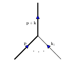
(a)

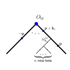
(b)

Figure 1: (a) A vertex with large incoming and outgoing momenta $p\sim\Lambda$. Dots represent omitted lines whose momenta add up to $\mathbf{k}-\mathbf{k}_{1}$. (b) A composite operator with two of the incoming momenta large and nearly opposite. All interactions along the large-momentum line yield local expressions in terms of the low-momentum incoming lines.

4.1 Renormalization and counter-terms

As seen above the perturbation theory and bias parametrization can be fully formulated in terms of $M^{ij}=\partial^{i}\mathbf{s}^{j}$. In this section we investigate the structure of counter-terms which must be added to the equations of motion of dark matter and to composite operators in order to remove the cutoff dependence of loop contributions to correlation functions.

Here we are solving an initial value problem; at each vertex lower order solutions (incoming legs) combine to give a higher order solution (outgoing line). When calculating a correlation function of $\delta_{g}$ several incoming lines can end at a composite operator. Cutoff dependence arises when at least a pair of initial fields are contracted and their momenta become of the order of cutoff $\Lambda$. One can argue that the counter-terms are all local functions of $M^{ij}$ and its spatial or temporal derivatives:

1. The perturbation theory vertices express the trace and curl of $M^{[n]}$ as a local function of lower order solutions [15]:

   $$\begin{split}\left(\nabla\times\mathbf{s}^{[n]}\right)^{i}=&\frac{1}{2}\sum_{0<m<n}\frac{n-2m}{n}\epsilon^{ijk}\left(M^{[m]}M^{[n-m]\,T}\right)_{jk}\,,\\ \nabla\cdot\mathbf{s}^{[n]}=&\frac{1}{2}\sum_{0<m<n}\frac{m^{2}+(n-m)^{2}+(n-3)/2}{n^{2}+(n-3)/2}[{\rm Tr}(M^{[m]}M^{[n-m]})-{\rm Tr}(M^{[m]}){\rm Tr}(M^{[n-m]})]\\ &-\frac{1}{6}\sum_{m_{1}+m_{2}+m_{3}=n}\frac{m_{1}^{2}+m_{2}^{2}+m_{3}^{2}+(n-3)/2}{n^{2}+(n-3)/2}\varepsilon^{ijk}\varepsilon^{lmn}M^{[m_{1}]}_{il}M^{[m_{2}]}_{jm}M^{[m_{3}]}_{kn}\,.\end{split}$$ (4.1)

   Non-localities appear when $M^{[n]}=\nabla\mathbf{s}^{(n)}$ is solved in terms of its symmetric and anti-symmetric parts:

   $$\mathbf{s}^{[n]}=\nabla^{-2}(-\nabla\times\nabla\times\mathbf{s}^{[n]}+\nabla\nabla\cdot\mathbf{s}^{[n]})\,.$$ (4.2)

   Thus, $M^{[n]}_{ij}$ is always given by $\partial_{i}\partial_{j}/\nabla^{2}$ acting on a product of $M^{[m]}$ with $m<n$.

2. If the outgoing line has a large momentum (this can happen except for the final vertex or the external operator), the $\nabla^{-2}$ operator can be Taylor expanded in powers of external soft momenta and becomes local. For instance, in the diagram of Fig. 1a the inverse Laplacian leads to a factor of $1/|\mathbf{p}+\mathbf{k}|^{2}$ which can be expanded in $k^{2}/p^{2}$.

3. When two or more high-momentum internal lines end in a finite momentum composite operator in $\delta_{g}$ one needs to add a counter-term to renormalize the operator. This counter-term depends on the soft initial fields in the diagram. Because of the previous point it can be written as a product of various $M^{[n]}$, and their derivatives suppressed by factors of $1/\Lambda$ (Fig. 1b). As before, these can be expressed in terms of $M$ its spatial, and convective time derivatives. The same argument also applies to interaction vertices of the dark matter field.

4. Renormalization should be done order by order: the above argument works only if all nested diagrams with several $\mathcal{O}(\Lambda)$ momenta combining into soft momenta are already renormalized by the addition of appropriate counter-terms at lower orders.

To summarize, all Lagrangian counter-terms necessary in order to renormalize a local operator are those in the list (3.14) (and their higher spatial derivatives). Therefore, local functions of $M^{ij}$ as well its spatial and convective time derivatives form a complete basis for the renormalized bias expansion.

5 Conclusions

We argued that galaxy bias can be formulated locally at the final time in an Eulerian fashion in terms of local observables given by contractions of $\partial_{i}\partial_{j}\Phi$ and its convective time derivatives. Time derivatives are necessary to include starting from the third order. Equivalently one can use a Lagrangian description, e.g. in terms of $M^{ij}=\partial_{q}^{i}s^{j}$. There is one bias parameter corresponding to each scalar quantity that can be constructed from product of various terms $M^{[n]}_{ij}$ appearing in the perturbative solution of $M_{ij}$. There is an analogous Eulerian operator for everyone of those. The complete list up to fourth order is given in Eq. (2.21) and Eq. (3.14). Then, when including all bias parameters in this list at a given order, “Eulerian” and “Lagrangian” biasing are merely different equivalent formulations with the same physical content. These claims were checked in an explicit third order calculation. Crucially, we also argued that the list of operators is closed under renormalization. The same rules can be used to construct a basis for the counter-terms in the EFT of the dark matter fluid.

A corollary of these considerations is that velocity bias can only enter through higher spatial derivative terms. At lowest order in spatial derivatives, tracers and matter have to be comoving in the absence of long-wavelength entropic perturbations. In other words, velocity biases of the type $\mathbf{v}_{g}=b_{v}\mathbf{v}+b_{v\delta}\delta\,\mathbf{v}$ and so on are prohibited by the equivalence principle in the absence of entropic perturbations (which however can exist in standard cosmology for example in the form of baryon-dark matter relative velocities [16]).

Up to third order the proposed list of operators agrees with [1, 8, 2]. However, beyond that one needs to include higher time derivatives and just working with local expressions made of gravitational and velocity potentials would be insufficient. On the other hand, our parametrization is more concise than that of [6]. Promoting all the bias coefficients to time integrals over history leads to redundancies in a perturbative approach. Only a subset of operators involving convective time derivatives are required at any given order to build a complete basis.

Appendix A Connection between velocity dispersion and tidal tensor

Here we show that the velocity dispersion $\partial_{i}v_{j}$ can be expressed perturbatively in terms of $\partial_{i}\partial_{j}\phi$ and its convective time derivatives. We start by taking a spatial derivative of the Euler equation:

$$\partial_{\tau}\partial_{i}v_{j}+(\mathbf{v}\cdot\nabla)\partial_{i}v_{j}+\partial_{i}v_{k}\partial_{k}v_{j}+\mathcal{H}\partial_{i}v_{j}=-\partial_{i}\partial_{j}\phi\,.$$ (A.1)

Next, we substitute the perturbative solutions for $\partial_{i}\partial_{j}\phi$ and $\partial_{i}v_{j}$ in terms of Lagrangian operators $(\partial_{i}\partial_{j}\phi)_{\rm lgr}^{[n]}(\mathbf{q})$ and $(\partial_{i}v_{j})_{\rm lgr}^{[n]}(\mathbf{q})$. The convective time derivative on the l.h.s. reduces to an ordinary time derivative and we obtain an algebraic equation which can be solved perturbatively for $(\partial_{i}v_{j})_{\rm lgr}^{[n]}$ in terms of $(\partial_{i}\partial_{j}\phi)_{\rm lgr}^{[m]}$ with $m\leq n$. The latter can be solved in terms of zeroth to $n-1^{st}$ convective time-derivatives of $\partial_{i}\partial_{j}\phi(\mathbf{x},\tau)$ and therefore the same is true for $\partial_{i}v_{j}(\mathbf{x},\tau)$ up to any order $n$.

Appendix B Tracer with instantaneous formation at third order

The “convective SPT” system Eqs. (2.5)–(2.7) can be written in compact form as

$$\frac{{\rm D}}{{\rm d}\tau}\mathbf{\Psi}=\> -\mathbf{\sigma}\cdot\mathbf{\Psi}+\mathbf{S}\quad\mbox{where}$$ (B.1)

$$\mathbf{\Psi}(\mathbf{x},\tau)=\left(\begin{array}[]{c}\delta_{g}(\mathbf{x},\tau)\\ \delta(\mathbf{x},\tau)\\ \theta(\mathbf{x},\tau)\end{array}\right);\quad\mathbf{\sigma}(\tau)=\> \left(\begin{array}[]{ccc}0&0&1\\ 0&0&1\\ 0&\frac{3}{2}\Omega_{m}\mathcal{H}^{2}&\mathcal{H}\end{array}\right);\quad\mathbf{S}(\mathbf{x},\tau)=\left(\begin{array}[]{c}-\delta_{g}\,\theta\\ -\delta\,\theta\\ -(\partial_{i}\mathbf{v}_{j})^{2}\end{array}\right)\,.$$ (B.11)

The fact that $\mathbf{\sigma}$ is degenerate already shows that the three equations are not really coupled, but rather the equation for $\delta_{g}$ can be integrated separately. However, Eq. (B.1) allows for a convenient compact derivation of both $\delta$ and $\delta_{g}$. Note that since we integrate the system along the fluid flow, our expressions contain exclusively invariant operators. For this reason, we will drop the subscript “bi” in the majority of this appendix for clarity.

B.1 Source term

Before we can integrate Eq. (B.1), we have to carefully consider the source term, in particular the third component $\mathbf{S}_{3}=(\partial_{i}\mathbf{v}_{j})^{2}$, where the derivative is with respect to Eulerian coordinate $\mathbf{x}$. This is nonlocally related to the degrees of freedom $\delta,\,\theta$ themselves. For this, we use a trick (see also Sec. 3), namely the fact that $\mathbf{v}$ is given by $\dot{\mathbf{s}}$ (as in the main text, dots stands for convective derivatives ${\rm D}/{\rm d}\tau$). Further, we need to transform the derivative from $\mathbf{x}$ to the fluid flow or Lagrangian coordinate $\mathbf{q}$ via

$$\partial_{x}^{i}=\left[\mathbf{1}+\mathbf{M}\right]^{-1}{}^{i}_{\ j}\partial_{q}^{j}\,,$$ (B.12)

where $\mathbf{M}^{ij}=\partial_{q}^{i}\mathbf{s}^{j}$. At second order, we then obtain

$$\partial_{x}^{i}\mathbf{v}^{j}=\left[\partial_{q}^{i}+(\partial_{q}^{i}\mathbf{s}_{k})\partial_{q}^{k}\right]\dot{\mathbf{s}}^{j}+\mathcal{O}(3)\,.$$ (B.13)

Here, the l.h.s is at $(\mathbf{x},\tau)$ while the r.h.s is at $(\mathbf{q},\tau)$ which are related through $\mathbf{x}=\mathbf{q}+\mathbf{s}(\mathbf{q},\tau)$. We then obtain at first and second order

$$\partial_{x}^{i}\mathbf{v}^{j}\Big{|}_{[1]}=\> \partial_{q}^{i}\dot{\mathbf{s}}_{[1]}^{j}$$

$$\partial_{x}^{i}\mathbf{v}^{j}\Big{|}_{[2]}=\> \partial_{q}^{i}\dot{\mathbf{s}}_{[2]}^{j}-(\partial_{q}^{i}\mathbf{s}_{[1]}^{k})\partial_{q,k}\mathbf{s}_{[1]}^{j}\,.$$ (B.14)

As a consistency check of the second order result, we can easily verify that the trace of the expression recovers $\theta^{[2]}_{{\rm lgr}}$, the invariant part of the velocity divergence at second order, i.e.

$$\delta_{ij}\partial_{x}^{i}\mathbf{v}^{j}\Big{|}_{[2]}=-a\,\dot{a}\left[\frac{13}{21}(\delta^{[1]})^{2}+\frac{4}{7}(K_{ij}^{[1]})^{2}\right]_{\tau_{0}}\,.$$ (B.15)

With these expressions, we can construct source terms that are purely in terms of Lagrangian derivatives. Note that at each order, we only need the displacement to one order less, since the source term is quadratic. In the following, all spatial derivatives will be with respect to $\mathbf{q}$. Pulling out $a$ factors for convenience, the third component of the source term is at first and second order given by:

$$(\mathbf{S}^{[1]})_{3}=\> -\dot{a}{}^{2}(\tau)\left[(K^{[1]})^{2}+\frac{1}{3}(\delta^{[1]})^{2}\right]_{\tau_{0}}$$

$$(\mathbf{S}^{[2]})_{3}=\> 2a\,\dot{a}{}^{2}(\tau)\left[-\frac{2}{3}\delta^{[1]}\sigma^{[2]}-2K^{[1]}_{ij}\mathcal{D}^{ij}\sigma^{[2]}+\frac{1}{9}(\delta^{[1]})^{3}+\delta^{[1]}(K^{[1]})^{2}+(K^{[1]})^{3}\right]_{\tau_{0}}\,.$$ (B.16)

Here and in the following, we let $K^{n}$ stand for ${\rm Tr}[K_{ij}^{n}]$. $\sigma_{[2]}\equiv\mathbf{\nabla}_{q}\cdot\mathbf{s}_{[2]}$ is given by

$$\sigma^{[2]}=\> \frac{1}{2}\left[-\frac{2}{7}(\delta^{[1]})^{2}+\frac{3}{7}(K^{[1]})^{2}\right]\,.$$ (B.17)

These are sufficient to obtain second and third order results, respectively.

B.2 Solution

We define the matrix $\mathbf{A}$ as the solution to the matrix ODE with boundary condition

$$\partial_{\tau}\mathbf{A}(\tau,\tau_{i})+\sigma(\tau)\mathbf{A}(\tau,\tau_{i})=0;\quad\mathbf{A}(\tau,\tau)=\mathbf{1}\,.$$ (B.18)

For matter, we seek the solution to the subset $i=2,3$ of Eq. (B.1) with inital conditions at $\tau\to 0$ given by linear theory. This yields

$$\left[\mathbf{\Psi}\right]_{i=2,3}(\mathbf{x},\tau)=\left[\mathbf{\Psi}^{[1]}\right]_{i=2,3}(\mathbf{x},\tau)+\int_{0}^{\tau}{\rm d}\tau^{\prime}\>\left[\mathbf{A}(\tau,\tau^{\prime})\mathbf{S}(\mathbf{x}_{\rm fl}(\tau^{\prime}),\,\tau^{\prime})\right]_{i=2,3}\,.$$ (B.19)

The linear solution for matter is given by

$$\left[\mathbf{\Psi}^{[1]}\right]_{i=2,3}(\mathbf{x},\tau)=\left(\begin{array}[]{c}a(\tau)\delta_{[1]}(\mathbf{x}_{\rm fl}(0))\\ -\dot{a}(\tau)\delta_{[1]}(\mathbf{x}_{\rm fl}(0))\end{array}\right)=\left(\begin{array}[]{c}a(\tau)\\ -\dot{a}(\tau)\end{array}\right)\delta_{1}(\mathbf{q})\,,$$ (B.20)

where $\delta_{1}(\mathbf{q})$ is the linear density field as function of the Lagrangian coordinate, extrapolated to the time $\tau_{0}$ where $a(\tau_{0})=1$ following standard convention. As we will see below, Eq. (B.19) leads to the standard SPT result for matter for the invariant terms, while we have not expanded in the displacement yet. Expanding the displacements to the same perturbative order then yields exactly the non-invariant (displacement) terms of SPT.

We now consider the conserved tracer at $\tau\geq\tau_{*}$. The initial condition for the integration of the full set of equations Eq. (B.1) is given by Eq. (2.28),

$$\mathbf{\Psi}(\mathbf{x}_{*},\tau_{*})=\left(\begin{array}[]{c}\delta_{g}^{*}\\ \delta^{*}\\ \theta^{*}\end{array}\right)\,;\quad\delta_{g}^{*}=\> \sum_{n=1}^{3}\frac{b_{n}^{*}}{n!}[\delta^{*}]^{n}+\sum_{n=2}^{3}\frac{b_{K^{n}}^{*}}{n!}{\rm Tr}\left[(K_{ij}^{*})^{n}\right]+\frac{1}{6}b_{\delta K^{2}}\delta^{*}\>{\rm Tr}\left[(K_{ij}^{*})^{2}\right]$$ (B.24)

$$+\epsilon^{*}_{0}+\epsilon^{*}_{\delta}\delta^{*}+\frac{1}{2}\epsilon^{*}_{\delta^{2}}[\delta^{*}]^{2}+\frac{1}{2}\epsilon^{*}_{K^{2}}{\rm Tr}\left[(K_{ij}^{*})^{2}\right]\,,$$ (B.25)

where a superscript $*$ indicates that a quantity is evaluated at $\mathbf{x}_{*}=\mathbf{x}_{\rm fl}(\tau_{*})$ and $\tau_{*}$. The quantities $\delta^{*},\,\theta^{*}$ are obtained by integrating Eq. (B.19) up to $\tau_{*}$. The particular solution to Eq. (B.1) with Eq. (B.25) is then given by

$$\mathbf{\Psi}(\mathbf{x},\tau)=\mathbf{A}(\tau,\tau_{*})\left(\begin{array}[]{c}\delta_{g}^{*}\\ \delta^{*}\\ \theta^{*}\end{array}\right)+\int_{\tau_{*}}^{\tau}{\rm d}\tau^{\prime}\>\mathbf{A}(\tau,\tau^{\prime})\mathbf{S}(\mathbf{x}_{\rm fl}(\tau^{\prime}),\,\tau^{\prime})\,.$$ (B.26)

The interpretation of Eq. (B.26) is clear: the density and velocity of the fluid and tracer at position $(\mathbf{x},\tau)$ is given by an integral of the source term over the fluid trajectory.

In the following, we assume an Einstein-de Sitter Universe ($\Omega_{m}=1$), which yields

$$\mathbf{\sigma}(\tau)=\left(\begin{array}[]{ccc}0&0&1\\ 0&0&1\\ 0&\frac{3}{2}H_{0}^{2}a^{-1}&H_{0}a^{-1/2}\end{array}\right)=\left(\begin{array}[]{ccc}0&0&1\\ 0&0&1\\ 0&6/\tau^{2}&2/\tau\end{array}\right)\,.$$ (B.27)

The expression for $\mathbf{A}$ is easy to derive since we know that the growing and decaying modes of the linear density field corresponding to the homogeneous solution are $\propto\tau^{2}$ and $\tau^{-3}$, respectively. The linear solution is given by

$$\mathbf{\Psi}^{[1]}(\mathbf{x},\tau)=a(\tau)\left(\begin{array}[]{c}b_{1}^{E}(\tau)\\ 1\\ -\mathcal{H}(\tau)\end{array}\right)\delta_{1}(\mathbf{q})+\left(\begin{array}[]{c}\epsilon_{0}^{*}\\ 0\\ 0\end{array}\right)\,,$$ (B.28)

where

$$b_{1}^{E}(\tau)\equiv(b_{1}^{*}-1)\frac{a(\tau_{*})}{a(\tau)}+1\,.$$ (B.29)

We can then perform the usual replacement of $a(\tau)\to D(\tau)$ to move from Einstein-de Sitter to $\Lambda$CDM. Thus,

$$\frac{a(\tau_{*})}{a(\tau)}\to\frac{D(\tau_{*})}{D(\tau)}\equiv D_{*}\,.$$ (B.30)

B.3 Second and third order results

Since the linear solution for $(\mathbf{x},\tau)$ where $\mathbf{x}=\mathbf{x}_{\rm fl}(\tau)$ is a function of $\mathbf{q}=\mathbf{x}_{\rm fl}(0)$, the second order source term at $(\mathbf{x}_{\rm fl}(\tau^{\prime}),\tau^{\prime})$ integrated over in Eq. (B.26) is only a function of $\mathbf{q}$ and $\tau^{\prime}$, so that the integral can be straightforwardly evaluated. This in fact holds order by order. At second order, we have

$$\mathbf{S}^{[2]}(\mathbf{x}_{\rm fl}(\tau^{\prime}),\,\tau^{\prime})=\left(\begin{array}[]{c}-\delta_{g}^{[1]}\theta^{[1]}\\ -\delta^{[1]}\theta^{[1]}\\ -\left[(\dot{K}^{[1]})^{2}+\frac{1}{3}(\dot{\delta}^{[1]})^{2}\right]\end{array}\right)_{\tau^{\prime},\,\mathbf{q}}\,.$$ (B.31)

Performing the integral yields

$$\mathbf{\Psi}^{[2]}(\mathbf{x},\tau)=\left(\begin{array}[]{c}b_{1}^{E}(\tau)\delta^{[2]}+b_{2}^{E}(\tau)(\delta^{[1]})^{2}/2+b_{K^{2}}^{E}(\tau)(K_{[1]}^{ij})^{2}/2+\epsilon^{E}_{\delta}(\tau)\delta^{[1]}\\ a^{2}(\tau)\left[\frac{17}{21}(\delta^{[1]})^{2}+\frac{2}{7}(K_{[1]}^{ij})^{2}\right]\\ -a(\tau)\dot{a}(\tau)\left[\frac{13}{21}(\delta^{[1]})^{2}+\frac{4}{7}(K_{[1]}^{ij})^{2}\right]\end{array}\right)_{\mathbf{q}}\,,$$ (B.32)

where we have defined second order Eulerian bias parameters

$$b_{2}^{E}(\tau)=\> b_{2}^{*}D_{*}^{2}-\frac{8}{21}(b_{1}^{*}-1)D_{*}(D_{*}-1)$$

$$b_{K^{2}}^{E}(\tau)=\> b_{K^{2}}^{*}D_{*}^{2}+\frac{4}{7}(b_{1}^{*}-1)D_{*}(D_{*}-1)\,,$$ (B.33)

and the Eulerian stochasticity

$$\epsilon^{E}_{\delta}(\tau)=\epsilon^{*}_{\delta}D_{*}-(D_{*}-1)\epsilon^{*}_{0}\,.$$ (B.34)

Note that $\epsilon^{E}_{\delta}$ has one power of $D_{*}$ less than the other second order Eulerian quantities, since $\epsilon^{*}_{i}$ are defined at $\tau_{*}$.

As mentioned above, $\mathbf{\Psi}^{[2]}(\mathbf{x},\tau)$ is a local function of the matter fields and stochastic variables evaluated at $\mathbf{q}=\mathbf{x}_{\rm fl}(0)$, and we obtain only invariant terms. Moving to Eulerian position $\mathbf{x}$, the second order displacement term then simply adds to all three components of $\mathbf{\Psi}^{[2]}$ through

$$\mathbf{s}_{[1]}^{i}(\mathbf{x},\tau)\partial_{i}\mathbf{\Psi}^{[1]}|_{\mathbf{x}}\,.$$ (B.35)

At third order, we have

$$\mathbf{S}^{[2]}(\mathbf{x}_{\rm fl}(\tau^{\prime}_{,}\,\tau^{\prime})=\left(\begin{array}[]{c}-(\delta_{g}^{[1]}\theta^{[2]}+\delta_{g}^{[2]}\theta^{[1]})_{\tau^{\prime}}\\ -(\delta^{[1]}\theta^{[2]}+\delta^{[2]}\theta^{[1]})_{\tau^{\prime}}\\ 2a\,\dot{a}{}^{2}(\tau)\left[-\frac{2}{3}\delta^{[1]}\sigma^{[2]}-2K^{[1]}_{ij}\mathcal{D}^{ij}\sigma^{[2]}+\frac{1}{9}(\delta^{[1]})^{3}+\delta^{[1]}(K^{[1]})^{2}+(K^{[1]})^{3}\right]_{\tau_{0}}\end{array}\right)_{\mathbf{q}}\,.$$

Inserting this into Eq. (B.26), we correspondingly recover the invariant part of the third order matter density and velocity dispersion (see App. C),

$$\delta^{[3]}=\> \frac{341}{567}\delta^{3}+\frac{11}{21}K^{2}\delta+\frac{2}{9}K^{3}-\frac{4}{9}K^{ij}\mathcal{D}_{ij}\sigma^{[2]}$$

$$\theta^{[3]}=\> \frac{\dot{D}(\tau)}{D(\tau)}\left[\frac{71}{189}\delta^{3}+\frac{5}{7}K^{2}\delta+\frac{2}{3}K^{3}-\frac{4}{3}K^{ij}\mathcal{D}_{ij}\sigma^{[2]}\right]\,,$$ (B.36)

where all quantities on the r.h.s. are linear and evaluated at $\tau$. Notice that the prefactor of the $\delta^{3}$ term in $\delta^{[3]}$ is exactly the third-order coefficient of the perturbative expansion of spherical collapse in Einstein-de Sitter, as expected. For $\delta_{g}$, we obtain at third order

$$\delta_{g}^{[3]}(\mathbf{x},\tau)=\> b_{1}^{E}\delta^{[3]}+b_{2}^{E}\delta^{[1]}\delta^{[2]}+b_{K^{2}}^{E}K^{[1]}K^{[2]}+\frac{1}{6}\left[b_{3}^{E}(\delta^{[1]})^{3}+b_{K^{3}}^{E}(K^{[1]})^{3}+b_{\delta K^{2}}\delta^{[1]}(K^{[1]})^{2}\right]$$

$$+\frac{1}{6}b_{\rm nloc}^{E}K^{[1]}_{ij}\mathcal{D}^{ij}\left[(\delta^{[1]})^{2}-\frac{3}{2}(K^{[1]})^{2}\right]$$

$$+\epsilon_{\delta}^{E}\delta^{[2]}+\frac{1}{2}\epsilon_{\delta^{2}}^{E}(\delta^{[1]})^{2}+\frac{1}{2}\epsilon_{K^{2}}^{E}(K^{[1]})^{2}\,,$$ (B.37)

where the third order final-time bias parameters are given by

$$b_{3}^{E}(\tau)=\> b_{3}^{*}D_{*}^{3}+\left[(b_{1}^{*}-1)\frac{4}{1323}(199-35D_{*})+\frac{13}{7}b_{2}^{*}D_{*}\right]D_{*}(D_{*}-1)$$

$$b_{\delta K^{2}}^{E}(\tau)=\> b_{\delta K^{2}}^{*}D_{*}^{3}+\left[-(b_{1}^{*}-1)\frac{2}{49}(33+7D_{*})+\left(\frac{12}{7}b_{2}^{*}+3b_{K^{2}}^{*}\right)D_{*}\right]D_{*}(D_{*}-1)$$

$$b_{K^{3}}^{E}(\tau)=\> b_{K^{3}}^{*}D_{*}^{3}+\left[(b_{1}^{*}-1)\frac{4}{21}(-11+7D_{*})+6b_{K^{2}}^{*}D_{*}\right]D_{*}(D_{*}-1)$$

$$b_{\rm nloc}^{E}(\tau)=\> \left[(b_{1}^{*}-1)\left(-\frac{8}{21}\right)\left(\frac{23}{7}-D_{*}\right)+\frac{20}{7}b_{K^{2}}^{*}D_{*}\right]D_{*}(D_{*}-1)\,.$$ (B.38)

We can see that, as expected, all corrections to the bias parameters at $\tau_{*}$ disappear for $D_{*}\to 1$ and $D_{*}\to 0$ (unless $b_{X}^{*}$ diverge in the latter limit, which is usually assumed for Lagrangian biasing). $b_{\rm nloc}^{E}$ multiplies third order terms which cannot be expressed locally in terms of the linear density and tidal field. They are exactly of the structure discussed in Sec. 2. Moreover, using that

$$\mathcal{D}_{ij}\sigma^{[2]}=-\frac{1}{7}\mathcal{D}_{ij}\left[\delta^{2}-\frac{3}{2}K^{2}\right]\,,$$ (B.39)

we see that, to the order we work in, we can equivalently write Eq. (B.37) as

$$\delta_{g}^{[3]}(\mathbf{x},\tau)=\> b_{1}^{E}\delta^{[3]}+b_{2}^{E}\delta^{[1]}\delta^{[2]}+b_{K^{2}}^{E}K^{[1]}K^{[2]}+\frac{1}{6}\left[b_{3}^{E}(\delta^{[1]})^{3}+b_{K^{3}}^{E}(K^{[1]})^{3}+b^{E}_{\delta K^{2}}\delta^{[1]}(K^{[1]})^{2}\right]$$

$$+\frac{1}{6}\left(-7b_{\rm nloc}^{E}\right)K_{[1]}^{ij}M^{[2]}_{ij}\,,$$ (B.40)

where

$$M^{[2]}_{ij}=\frac{\partial_{q}^{i}\partial_{q}^{j}}{\nabla_{q}^{2}}\sigma^{[2]}$$ (B.41)

is the second order Lagrangian distortion tensor. This can be equivalently written in terms of $M^{\prime}_{ij}-M_{ij}$ (see Sec. 3.2). The Eulerian stochasticity terms at third order become

$$\epsilon_{\delta^{2}}^{E}(\tau)=\> \epsilon^{*}_{\delta^{2}}D_{*}^{2}-\frac{8}{21}(\epsilon_{\delta}^{*}-\epsilon_{0}^{*})D_{*}(D_{*}-1)$$

$$\epsilon_{K^{2}}^{E}(\tau)=\> \epsilon^{*}_{K^{2}}D_{*}^{2}+\frac{4}{7}(\epsilon_{\delta}^{*}-\epsilon_{0}^{*})D_{*}(D_{*}-1)\,.$$ (B.42)

Finally, in order to obtain the density at a fixed order in standard Eulerian perturbation theory, we need to expand the argument of the various orders of $\mathbf{\Psi}$. Let us define $\mathbf{\Psi}^{E}$ through

$$\mathbf{\Psi}^{E}(\mathbf{x})=\mathbf{\Psi}(\mathbf{x}-\mathbf{s}[\mathbf{q},\tau])\,.$$ (B.43)

$\mathbf{\Psi}$ on the r.h.s. contains all invariant terms, which we have worked out here. We now perform a Taylor expansion in $\mathbf{s}$ as well as a perturbative expansion of $\mathbf{s}$, noting that $\mathbf{s}$ is itself a function of the Lagrangian rather than Eulerian position. We obtain

$$\mathbf{\Psi}^{E}=\> \mathbf{\Psi}^{[3]}-\mathbf{s}_{[1]}^{i}\partial_{i}\mathbf{\Psi}^{[2]}-\left[\mathbf{s}_{[2]}^{i}-\mathbf{s}_{[1]}^{j}(\partial_{j}\mathbf{s}_{[1]}^{i})\right]\partial_{i}\mathbf{\Psi}^{[1]}+\frac{1}{2}\mathbf{s}_{[1]}^{i}\mathbf{s}_{[1]}^{j}\partial_{i}\partial_{j}\mathbf{\Psi}^{[1]}\,,$$ (B.44)

where on the r.h.s. all quantities are evaluated at $\mathbf{x},\,\tau$, and $\mathbf{\Psi}^{[1]}$, $\mathbf{\Psi}^{[2]}$, $\mathbf{\Psi^{[3]}}$ are given in Eq. (B.28), Eq. (B.32), and Eqs. (B.36)–(B.37), respectively.

An alternative derivation of these results can be obtained as follows (see Sec. III of Ref. [8]). For conserved tracers, the continuity equation Eq. (2.7) and absence of velocity bias at lowest order in derivatives (Sec. 2.5) imply

$$-\theta=\frac{1}{1+\delta_{g}}\frac{{\rm D}\delta_{g}}{{\rm d}\tau}=\frac{1}{1+\delta}\frac{{\rm D}\delta}{{\rm d}\tau}\,.$$ (B.45)

This can be immediately integrated to yield

$$\ln[1+\delta_{g}(\mathbf{x}_{\rm fl}(\tau),\tau)]=\ln[1+\delta(\mathbf{x}_{\rm fl}(\tau),\tau)]+F[\mathbf{x}_{\rm fl}(\tau_{*})]\,,$$ (B.46)

where $F$ is a function of space only, which we have chosen to be defined on the formation time slice $\tau_{*}$. Evaluating Eq. (B.46) at $\tau_{*}$, we obtain

$$F(\mathbf{x}_{*})=\ln\left[\frac{1+\delta_{g}(\mathbf{x}_{*},\tau_{*})}{1+\delta(\mathbf{x}_{*},\tau_{*})}\right]\,.$$ (B.47)

One can now insert the bias expansion Eq. (B.25) and expand Eq. (B.46) to the desired order.

Appendix C Matter density perturbation at third order

For reference, we now show how to obtain an expression for the third order density field in real space, with invariant and non-invariant terms explicitly separated, from standard perturbation theory expressions. We start from the symmetrized third-order perturbation theory kernel [17],

$$F_{3}(\mathbf{k}_{1},\mathbf{k}_{2},\mathbf{k}_{3})=\> \frac{2}{54}k_{123}^{2}\left[\frac{\mathbf{k}_{1}\cdot\mathbf{k}_{23}}{k_{1}^{2}k_{23}^{2}}G_{2}(\mathbf{k}_{2},\mathbf{k}_{3})+2\>\rm perm.\right]$$

$$+\frac{7}{54}\mathbf{k}_{123}\cdot\left[\frac{\mathbf{k}_{12}}{k_{12}^{2}}G_{2}(\mathbf{k}_{1},\mathbf{k}_{2})+2\>\rm perm.\right]$$

$$+\frac{7}{54}\mathbf{k}_{123}\cdot\left[\frac{\mathbf{k}_{1}}{k_{1}^{2}}F_{2}(\mathbf{k}_{2},\mathbf{k}_{3})+2\>\rm perm.\right]\,,$$ (C.1)

where $F_{2}$ and $G_{2}$ are given by

$$F_{2}(\mathbf{k}_{1},\mathbf{k}_{2})=\> \frac{5}{7}+\frac{2}{7}\frac{(\mathbf{k}_{1}\cdot\mathbf{k}_{2})^{2}}{k_{1}^{2}k_{2}^{2}}+\frac{1}{2}\mathbf{k}_{1}\cdot\mathbf{k}_{2}\left(k_{1}^{-2}+k_{2}^{-2}\right)$$

$$G_{2}(\mathbf{k}_{1},\mathbf{k}_{2})=\> \frac{3}{7}+\frac{4}{7}\frac{(\mathbf{k}_{1}\cdot\mathbf{k}_{2})^{2}}{k_{1}^{2}k_{2}^{2}}+\frac{1}{2}\mathbf{k}_{1}\cdot\mathbf{k}_{2}\left(k_{1}^{-2}+k_{2}^{-2}\right)\,.$$ (C.2)

Transforming the Fourier integral over Eq. (C.1) into real space, we obtain after some algebra

$$\delta^{[3]}=\> \frac{341}{567}\delta^{3}+\frac{71}{189}\delta\,K^{2}-\frac{145}{189}\delta\,\mathbf{s}^{i}\partial_{i}\delta-\frac{11}{63}\mathbf{s}^{i}\partial_{i}K^{2}+\frac{1}{2}\mathbf{s}^{i}(\partial_{i}\mathbf{s}^{j})\partial_{j}\delta+\frac{1}{2}\mathbf{s}^{i}\mathbf{s}^{j}\partial_{i}\partial_{j}\delta$$

$$+\frac{1}{2}\frac{\partial^{i}}{\nabla^{2}}\left[\frac{13}{21}\delta^{2}+\frac{4}{7}[K_{jk}]^{2}-\mathbf{s}^{j}\partial_{j}\delta\right]\partial_{i}\delta+\frac{2}{9}K_{ij}\mathcal{D}^{ij}\left[\frac{13}{21}\delta^{2}+\frac{4}{7}[K_{ij}]^{2}-\mathbf{s}^{j}\partial_{j}\delta\right]\,.$$ (C.3)

Here and in the following, all terms without further sub/superscripts denote linear order quantities.

We are interested in separating terms that involve the displacement (non-invariant) and those that do not (invariant) in Eq. (C.3). For this, we need to manipulate the terms which contain a displacement inside the inverse Laplacian. Using a suitable reordering of $k$ factors in Fourier space, one can easily prove the following relations:

$$\frac{\partial^{i}\partial^{j}}{\nabla^{2}}\left[\mathbf{s}^{j}\partial_{j}\delta\right]=\> -\frac{1}{2}\partial^{i}\partial^{j}[\mathbf{s}^{2}]+\frac{\partial^{i}\partial^{j}}{\nabla^{2}}\left[K^{2}+\frac{1}{3}\delta^{2}\right]$$

$$\frac{\partial^{i}}{\nabla^{2}}\left[\mathbf{s}^{j}\partial_{j}\delta\right]=\> -\frac{1}{2}\partial^{i}\left[\mathbf{s}^{2}\right]+\frac{\partial^{i}}{\nabla^{2}}\left[K^{2}+\frac{1}{3}\delta^{2}\right]=-\mathbf{s}^{k}(\partial_{k}\mathbf{s}^{i})+\frac{\partial^{i}}{\nabla^{2}}\left[K^{2}+\frac{1}{3}\delta^{2}\right]\,,$$ (C.4)

where we have used $\mathbf{s}^{i}=-(\partial^{i}/\nabla^{2})\delta$ to switch derivatives. This yields

$$K^{ij}\mathcal{D}_{ij}\left[\mathbf{s}^{j}\partial_{j}\delta\right]=\> -K^{3}-\frac{2}{3}\delta K^{2}+\frac{1}{2}\mathbf{s}^{k}\partial_{k}K^{2}+K^{ij}\mathcal{D}_{ij}\left[K^{2}+\frac{1}{3}\delta^{2}\right]$$

$$-\frac{\partial^{i}}{\nabla^{2}}\left[\frac{13}{21}\delta^{2}+\frac{4}{7}[K_{jk}]^{2}-\mathbf{s}^{j}\partial_{j}\delta\right]=\> -\frac{\partial^{i}}{\nabla^{2}}\left[\frac{2}{7}\delta^{2}-\frac{3}{7}K^{2}\right]-\mathbf{s}^{k}(\partial_{k}\mathbf{s}^{i})\,.$$ (C.5)

The second equation is the relation between second-order displacements at fixed Eulerian position (left-hand side), given by the time integral over $-(\partial^{i}/\nabla^{2})\theta^{[2]}$, and fixed Lagrangian position (first term on the right-hand side), precisely $2\mathbf{s}_{[2]}^{i}$. Inserting these relations into Eq. (C.3), we obtain

$$\delta^{[3]}=\> \delta^{[3]}_{{\rm lgr}}+\frac{1}{2}\frac{\partial^{i}}{\nabla^{2}}\left[\frac{2}{7}\delta^{2}-\frac{3}{7}K^{2}\right]\partial_{i}\delta+\mathbf{s}^{k}(\partial_{k}\mathbf{s}^{i})\partial_{i}\delta+\frac{1}{2}\mathbf{s}^{i}\mathbf{s}^{k}\partial_{i}\partial_{k}\delta-\mathbf{s}^{i}\partial_{i}\left[\frac{17}{21}\delta^{2}+\frac{2}{7}K^{2}\right]$$ (C.6)

$$\delta^{[3]}_{{\rm lgr}}=\> \frac{341}{567}\delta^{3}+\frac{11}{21}\delta K^{2}+\frac{2}{9}K^{3}+\frac{2}{9}K^{ij}\mathcal{D}_{ij}\left[\frac{2}{7}\delta^{2}-\frac{3}{7}K^{2}\right]\,,$$

where we have collected the invariant terms in $\delta^{[3]}_{{\rm lgr}}$. The remaining terms in Eq. (C.6) are the displacement or non-invariant terms. Using the notation defined above [Eq. (B.17)], we can write this as

$$\delta^{[3]}=\> -\mathbf{s}_{[2]}^{i}\partial_{i}\delta+\mathbf{s}^{k}(\partial_{k}\mathbf{s}^{i})\partial_{i}\delta+\frac{1}{2}\mathbf{s}^{i}\mathbf{s}^{k}\partial_{i}\partial_{k}\delta-\mathbf{s}^{i}\partial_{i}\delta^{[2]}_{{\rm lgr}}$$

$$+\frac{341}{567}\delta^{3}+\frac{11}{21}\delta K^{2}+\frac{2}{9}K^{3}-\frac{4}{9}K^{ij}\mathcal{D}_{ij}\sigma_{[2]}\,,$$ (C.7)

which agrees with Eq. (B.44) and Eq. (B.36) from the convective SPT approach.

References

- McDonald and Roy [2009] P. McDonald and A. Roy, JCAP 8, 20 (2009), 0902.0991.
- Assassi et al. [2014] V. Assassi, D. Baumann, D. Green, and M. Zaldarriaga, JCAP 8, 056 (2014), 1402.5916.
- Mo and White [1996] H. J. Mo and S. D. M. White, MNRAS 282, 347 (1996), arXiv:astro-ph/9512127.
- Matsubara [2008] T. Matsubara, Phys. Rev. D 78, 083519 (2008), 0807.1733.
- Schmidt et al. [2012] F. Schmidt, D. Jeong, and V. Desjacques, ArXiv e-prints (2012), 1212.0868.
- Senatore [2014] L. Senatore, ArXiv e-prints (2014), 1406.7843.
- Tegmark and Peebles [1998] M. Tegmark and P. J. E. Peebles, Astrophys. J. Lett. 500, L79 (1998), astro-ph/9804067.
- Chan et al. [2012] K. C. Chan, R. Scoccimarro, and R. K. Sheth, Phys. Rev. D 85, 083509 (2012), 1201.3614.
- Baldauf et al. [2012] T. Baldauf, U. Seljak, V. Desjacques, and P. McDonald, Phys.Rev. D86, 083540 (2012), 1201.4827.
- Sheth et al. [2013] R. K. Sheth, K. C. Chan, and R. Scoccimarro, Phys.Rev. D87, 083002 (2013), 1207.7117.
- Baldauf et al. [2014] T. Baldauf, L. Mercolli, M. Mirbabayi, and E. Pajer, ArXiv e-prints (2014), 1406.4135.
- Saito et al. [2014] S. Saito, T. Baldauf, Z. Vlah, U. Seljak, T. Okumura, et al. (2014), 1405.1447.
- Biagetti et al. [2014] M. Biagetti, V. Desjacques, A. Kehagias, and A. Riotto, Phys.Rev. D90, 045022 (2014), 1405.1435.
- Baumann et al. [2012] D. Baumann, A. Nicolis, L. Senatore, and M. Zaldarriaga, JCAP 7, 051 (2012), 1004.2488.
- Zheligovsky and Frisch [2014] V. Zheligovsky and U. Frisch, Journal of Fluid Mechanics 749, 404 (2014), 1312.6320.
- Tseliakhovich and Hirata [2010] D. Tseliakhovich and C. Hirata, Phys. Rev. D 82, 083520 (2010), 1005.2416.
- Bernardeau et al. [2002] F. Bernardeau, S. Colombi, E. Gaztañaga, and R. Scoccimarro, Phys. Rep. 367, 1 (2002), arXiv:astro-ph/0112551.