Understanding higher-order nonlocal halo bias at large scales
by combining the power spectrum with the bispectrum

Abstract

Understanding the relation between underlying matter distribution and biased tracers such as galaxies or dark matter halos is essential to extract cosmological information from ongoing or future galaxy redshift surveys. At sufficiently large scales such as the Baryon Acoustic Oscillation (BAO) scale, a standard approach for the bias problem on the basis of the perturbation theory (PT) is to assume the ‘local bias’ model in which the density field of biased tracers is deterministically expanded in terms of matter density field at the same position. The higher-order bias parameters are then determined by combining the power spectrum with higher-order statistics such as the bispectrum.

As is pointed out by recent studies, however, nonlinear gravitational evolution naturally induces nonlocal bias terms even if initially starting only with purely local bias. As a matter of fact, previous works showed that the second-order nonlocal bias term, which corresponds to the gravitational tidal field, is important to explain the characteristic scale-dependence of the bispectrum. In this paper we extend the nonlocal bias term up to third order, and investigate whether the PT-based model including nonlocal bias terms can simultaneously explain the power spectrum and the bispectrum of simulated halos in $N$-body simulations. The bias renormalization procedure ensures that only one additional term is necessary to be introduced to the power spectrum as a next-to-leading order correction, even if third-order nonlocal bias terms are taken into account. We show that the power spectrum, including density and momentum, and the bispectrum between halo and matter in $N$-body simulations can be simultaneously well explained by the model including up to third-order nonlocal bias terms at $k\raisebox{-2.15277pt}{$\>\stackrel{{\scriptstyle\textstyle<}}{{\sim}}\>$}0.1h$/Mpc. Also, the results are in a good agreement with theoretical predictions of a simple coevolution picture, although the agreement is not perfect. These trend can be found for a wide range of halo mass, $0.7\raisebox{-2.15277pt}{$\>\stackrel{{\scriptstyle\textstyle<}}{{\sim}}\>$}M_{\rm halo}\,[10^{13}M_{\odot}/h]\raisebox{-2.15277pt}{$\>\stackrel{{\scriptstyle\textstyle<}}{{\sim}}\>$}20$ at various redshifts, $0\leq z\leq 1$. These demonstrations clearly show a failure of the local bias model even at such large scales, and we conclude that nonlocal bias terms should be consistently included in order to accurately model statistics of halos.

I Introduction

Precise observation of the early universe has been well established by measurements of temperature and polarization anisotropy of the Cosmic Microwave Background (CMB) such as Wilkinson Microwave Anisotropy Probe (WMAP) Komatsu et al. (2009, 2011); Hinshaw et al. (2013) or Planck Planck Collaboration et al. (2013). Now we enter a new era of precision cosmology by getting in hand various kinds of large-scale structure measurements in late-time universe, mainly aiming at unveiling dark universe (see Weinberg et al. (2013) for a recent review). In particular, clustering of galaxies in a three dimensional map of the universe offers us a lot of fruitful cosmological information via the Baryon Acoustic Oscillations (BAOs), Redshift-Space Distortion (RSD), or the shape of galaxy clustering statistics such as the power spectrum and the bispectrum (for an encompassing review, see Bernardeau et al. (2002)). As a matter of fact, recent works by Baryon Oscillation Spectroscopic Survey (BOSS) Schlegel et al. (2009) in Sloan Digital Sky Survey III (SDSS-III) Eisenstein et al. (2011) or WiggleZ survey Drinkwater et al. (2010) have already accomplished very accurate measurements of such signals Anderson et al. (2013a); Reid et al. (2012); Anderson et al. (2013b); Samushia et al. (2013); Beutler et al. (2013, 2014); Zhao et al. (2013); Reid et al. (2014); Blake et al. (2011a, b, c, d, 2012); Contreras et al. (2013); Scrimgeour et al. (2012). Planned or near-future galaxy redshift surveys, which include Subaru Prime Focus Spectrograph (PFS) Survey Takada et al. (2012), Hobby-Eberly Telescope Dark Energy Experiment (HETDEX) Adams et al. (2011), Dark Energy Spectroscopic Instrument (DESI) Levi et al. (2013) and Euclid Laureijs et al. (2011), will continue to improve measurement accuracy at various redshift and scales.

In order to unlock full potential of cosmological information in the galaxy clustering, it is essential to understand the relation between underlying matter distribution and galaxies, known as the so-called galaxy bias problem. It is often assumed that galaxy distribution well traces underlying matter distribution which can be directly probed by cosmological $N$-body simulations. Given the fact that we do not have complete knowledge of galaxy formation scenario in nonlinear structure formation, it is a common practice to connect observed galaxy distribution to simulated dark matter halos. This approach is based on the halo model Cooray and Sheth (2002); Seljak (2000), and its associated techniques such as Halo Occupation Distribution (HOD) and Subhalo Abundance Matching (SHAM) (e.g., Behroozi et al. (2010); Reddick et al. (2012); Hearin and Watson (2013); Zentner et al. (2013)) are applied to somewhat small-scale galaxy clustering (typically $\sim\mathcal{O}(\text{0.1-10})\,$Mpc) (see e.g., Leauthaud et al. (2011); Tinker et al. (2013); Guo et al. (2014) and references therein for recent studies).

Even though dark matter halos can be easily constructed in $N$-body simulations, it is important to theoretically understand clustering of the halos, or halo bias, especially at large scales around BAOs ($\sim 150\,$Mpc), because the halo clustering is sensitive to underlying cosmology at the regimes (where, in other words, the two-halo term is dominant in the halo-model context). Some authors tried to formulate the halo or galaxy bias in parametric ways (see e.g., Cole et al. (2005); Tegmark et al. (2006); Yamamoto et al. (2010); Oka et al. (2014)) and showed a successful performance depending on their specific purpose, although it might be hard to be justified in more general situations. It is therefore desirable to develop an analytic formulation to describe the halo clustering in a physically-well motivated way. Perturbation theory (PT) is a natural approach along this direction, and, in the PT approach, the so-called ‘local bias’ model Kaiser (1984); Fry and Gaztanaga (1993) in which the density field of halos is deterministically Tailor-expanded in terms of matter density field at the same position as

$$\delta_{\rm h}(\mbox{\boldmath$x$})=\sum_{n}\frac{b_{n}}{n!}\delta_{\rm m}(\mbox{\boldmath$x$})^{n},$$ (1)

where $b_{n}$ is the bias coefficient at $n$-th order, and $\delta_{\rm h}$ and $\delta_{\rm m}$ describes density fields of halos and matter, respectively. It is well known that the local bias model works well at linear order to some extent Kaiser (1984), and the fitting formula for the halo mass function is calibrated so that it also consistently reproduces the linear bias value in simulations Sheth and Tormen (1999); Tinker et al. (2008). However, a couple of issues in the model have been recently pointed out. First of all, the model prefers different values of nonlinear bias parameter like $b_{2}$ for the halo power spectrum and the bispectrum Pollack et al. (2012, 2013), although the model looks well fitted to the spectra by properly choosing nonlinear bias parameters (see e.g. Jeong and Komatsu (2009); Saito et al. (2011); Nishizawa et al. (2012)). In addition, the authors McDonald and Roy (2009); Matsubara (2011); Baldauf et al. (2012); Chuen Chan et al. (2012) show that nonlinear gravitational evolution naturally induces nonlocal terms, and there are clear evidences of such a term at least at second-order perturbation observed in the bispectrum in simulations Baldauf et al. (2012); Chuen Chan et al. (2012). These caveats clearly warn adopting the local bias model from a physical point of view.

In this paper we continue to study how well the bias model including nonlocal terms performs against the halo statistics in $N$-body simulations. In particular, we focus on how well such a model can simultaneously explain the power spectrum as well as the bispectrum which again cannot be realized in the simple local bias model. While the leading-order (i.e., tree-level) bispectrum requires only up to second-order perturbation, it is necessary to consider up to third order as a next-to-leading order correction in the power spectrum. The author McDonald (2006) showed that the bias renormalization procedure allows us to write down a physical expression for the halo statistics and the third-order local bias term is absorbed into the linear bias. As we will revisit later, Ref. McDonald and Roy (2009) shows that all the correction terms associated with the third-order nonlocal bias can be summarized into only one term. This bias renormalization approach has been recently readdressed in terms of the effective field theory by Assassi et al. (2014), and they also reached the same conclusion (see also Kehagias et al. (2013)). Thus we have in hand a very simple bias model on the basis of PT even if considering all the local and nonlocal terms up to third order. Then the natural question that arises is whether the simple bias model can well explain the simulated halo power spectrum as well, and also whether the fitted value of the bias parameter is consistent with what is physically expected. In order to answer these questions, we study the halo-matter statistics in a standard $\Lambda$CDM universe at a various halo-mass range and redshift. We jointly fit the PT model to the power spectrum together with the bispectrum. An advantage of focusing on the halo-matter statistics is that it is free from the stochastic bias Seljak et al. (2009); Kitaura:2014wo and the velocity bias Percival and Schäfer (2008); Desjacques and Sheth (2010); Desjacques et al. (2010); Baldauf:2014xy. We also investigate the cross spectrum between halo density and matter momentum which was recently studied in modeling the RSDs in the Distribution Function approach (see Seljak and McDonald (2011); Okumura et al. (2012a, b); Vlah et al. (2012, 2013); Blazek et al. (2013) for a series of papers) and should be simultaneously explained by the same bias values if the model works.

The outline of this paper is as follows. In §. II, we first revisit the argument in McDonald and Roy (2009) and summarize a model to describe the halo-matter power spectrum and the bispectrum including nonlocal terms up to third order. In particular, we extend the model to the cross power spectrum between halo density and matter momentum which can be easily measured from the simulations and can be used to study the bias model as well. In addition, we study a simple coevolution picture of dark matter and halo fluids and derive a third-order solution. In §. III we describe our simulation details and fitting procedure. We then show our results in §. IV in which the bias model is compared with halo-matter power spectra in detail. Finally we make a summary and conclusion in in §. V.

II The halo-matter cross statistics in the presence of nonlocal bias terms

In this section we explicitly write down expressions for the halo-matter power spectrum on the basis of the perturbation theory (PT), including nonlocal bias terms. For this purpose we revisit an procedure proposed by McDonald and Roy (2009) in which all the possible bias terms are introduced by symmetry arguments and can be properly renormalized. After we review exactly the same procedure in McDonald and Roy (2009) for the matter-density and halo-density power spectrum, we will extend it to the matter-momentum and halo-density cross spectrum in a similar manner. We also discuss the bispectrum and bias renormalization Baldauf et al. (2012). For readers unfamiliar with PT, we refer to Appendix. A where basic equations in the PT formalism and our notations are summarized. While we here focus on the cross power spectrum, we present expressions for the auto correlators in Appendix. A as well.

II.1 The halo-matter density power spectrum

Starting from Eq. (55) which includes all possible perturbations up to third order for the next-to-leading order calculation of the power spectrum (e.g., see Bernardeau et al. (2002)), the matter-halo density power spectrum is written as

$$P^{\rm hm}_{\,00}(k) = \;\;c_{\delta}P(k)+c_{\delta}P^{(13)}_{\delta\delta}(k)+c_{\delta}P^{(22)}_{\delta\delta}(k)$$ (2)

$$+\frac{34}{21}c_{\delta^{2}}\sigma^{2}P(k)+\frac{1}{2}c_{\delta^{3}}\sigma^{2}P(k)+\frac{1}{3}c_{\delta s^{2}}\sigma^{2}P(k)+\frac{1}{2}c_{\delta\epsilon^{2}}\sigma^{2}_{\epsilon}P(k)$$

$$+c_{\delta^{2}}\int\frac{d^{3}q}{(2\pi)^{3}}\,P(q)P(|\mbox{\boldmath$k$}-\mbox{\boldmath$q$}|)F^{(2)}_{\rm S}(\mbox{\boldmath$q$},\mbox{\boldmath$k$}-\mbox{\boldmath$q$})$$

$$+c_{s^{2}}\int\frac{d^{3}q}{(2\pi)^{3}}\,P(q)P(|\mbox{\boldmath$k$}-\mbox{\boldmath$q$}|)F^{(2)}_{\rm S}(\mbox{\boldmath$q$},\mbox{\boldmath$k$}-\mbox{\boldmath$q$})S^{(2)}(\mbox{\boldmath$q$},\mbox{\boldmath$k$}-\mbox{\boldmath$q$})$$

$$+2c_{s^{2}}P(k)\int\frac{d^{3}q}{(2\pi)^{3}}\,P(q)F^{(2)}_{\rm S}(-\mbox{\boldmath$q$},\mbox{\boldmath$k$})S^{(2)}(\mbox{\boldmath$q$},\mbox{\boldmath$k$}-\mbox{\boldmath$q$})$$

$$+2c_{st}P(k)\int\frac{d^{3}q}{(2\pi)^{3}}\,P(q)D^{(2)}_{\rm S}(-\mbox{\boldmath$q$},\mbox{\boldmath$k$})S^{(2)}(\mbox{\boldmath$q$},\mbox{\boldmath$k$}-\mbox{\boldmath$q$})$$

$$+2c_{\psi}P(k)\int\frac{d^{3}q}{(2\pi)^{3}}\,P(q)\left[\frac{3}{2}D^{(3)}_{\rm S}(\mbox{\boldmath$q$},-\mbox{\boldmath$q$},-\mbox{\boldmath$k$})-2F^{(2)}_{\rm S}(-\mbox{\boldmath$q$},\mbox{\boldmath$k$})D^{(2)}_{\rm S}(\mbox{\boldmath$q$},\mbox{\boldmath$k$}-\mbox{\boldmath$q$})\right],$$

where the superscript ‘h’ stands for a quantity for halos and the subscript ‘0’ stands for the zeroth moment of mass-wighted velocity. All the bias coefficients, $c_{n}$, are bare bias parameters, and do not necessarily have clear physical meaning as explained later. $P(k)$ denotes the linear matter power spectrum, and the r.m.s of the fluctuated matter field, $\sigma^{2}$, is defined by $\sigma^{2}\equiv\int q^{2}dq\,P(q)/(2\pi^{2})$. Note that the term involving the third-order tidal term, $s^{3}$, vanishes in this case. Ref. McDonald (2006) argued that the first and second lines in Eq. (2) can be renormalized to a physical linear bias as follows: in the limit of $k\to 0$, one finds

$$c_{\delta}P(k)+c_{\delta}P^{(13)}_{\delta\delta}(k)+c_{\delta}P^{(22)}_{\delta\delta}(k)+\frac{34}{21}c_{\delta^{2}}\sigma^{2}P(k)+\frac{1}{2}c_{\delta^{3}}\sigma^{2}P(k)+\frac{1}{3}c_{\delta s^{2}}\sigma^{2}P(k)+\frac{1}{2}c_{\delta\epsilon^{2}}\sigma^{2}_{\epsilon}P(k)$$ (3)

$$\xrightarrow[k\to 0]{} \left(c_{\delta}+\frac{34}{21}c_{\delta^{2}}\sigma^{2}+\frac{1}{2}c_{\delta^{3}}\sigma^{2}+\frac{1}{3}c_{\delta s^{2}}\sigma^{2}+\frac{1}{2}c_{\delta\epsilon^{2}}\sigma^{2}_{\epsilon}\right)P(k).$$

In the limit of $k\to 0$, all the terms proportional to $P(k)$ should behave as the linear bias parameter times the linear power spectrum $P(k)$, which means that all the terms in the bracket can be interpreted as a renormalized linear bias. The third-order local bias term, $c_{\delta^{3}}$, is thus renormalized into the linear bias and not necessary to be considered. Ref. McDonald and Roy (2009) further found that the fifth, sixth and seventh lines in Eq. (2), whose origins are the third-order nonlocal terms, can be renormalized in a similar manner into a linear bias and just one additional bias parameter. In order to see this, let us first separate out $k\to 0$ limit of these terms,

$$\int\frac{d^{3}q}{(2\pi)^{3}}\,P(q)F^{(2)}_{\rm S}(-\mbox{\boldmath$q$},\mbox{\boldmath$k$})S^{(2)}(\mbox{\boldmath$q$},\mbox{\boldmath$k$}-\mbox{\boldmath$q$})\to\frac{34}{63}\sigma^{2},$$ (4)

$$\int\frac{d^{3}q}{(2\pi)^{3}}\,P(q)D^{(2)}_{\rm S}(-\mbox{\boldmath$q$},\mbox{\boldmath$k$})S^{(2)}(\mbox{\boldmath$q$},\mbox{\boldmath$k$}-\mbox{\boldmath$q$})\to-\frac{8}{63}\sigma^{2},$$ (5)

$$\int\frac{d^{3}q}{(2\pi)^{3}}\,P(q)\left[\frac{3}{2}D^{(3)}_{\rm S}(\mbox{\boldmath$q$},-\mbox{\boldmath$q$},-\mbox{\boldmath$k$})-2F^{(2)}_{\rm S}(-\mbox{\boldmath$q$},\mbox{\boldmath$k$})D^{(2)}_{\rm S}(\mbox{\boldmath$q$},\mbox{\boldmath$k$}-\mbox{\boldmath$q$})\right]\to 0.$$ (6)

These terms thus behaves as constants at $k\to 0$ and hence can be renormalized to linear bias parameters just as Eq. (3). In addition, Ref. McDonald and Roy (2009) found that these integrals exactly match each other and behaves as a filter function, once constants in $k\to 0$ limit are separated out and normalization factors are properly chosen,

$$\int\frac{d^{3}q}{(2\pi)^{3}}\,P(q)F^{(2)}_{\rm S}(-\mbox{\boldmath$q$},\mbox{\boldmath$k$})S^{(2)}(\mbox{\boldmath$q$},\mbox{\boldmath$k$}-\mbox{\boldmath$q$})=-\frac{8}{21}\sigma^{2}_{3}(k)+\frac{34}{63}\sigma^{2},$$ (7)

$$\int\frac{d^{3}q}{(2\pi)^{3}}\,P(q)D^{(2)}_{\rm S}(-\mbox{\boldmath$q$},\mbox{\boldmath$k$})S^{(2)}(\mbox{\boldmath$q$},\mbox{\boldmath$k$}-\mbox{\boldmath$q$})=\frac{16}{105}\sigma^{2}_{3}(k)-\frac{8}{63}\sigma^{2},$$ (8)

$$\int\frac{d^{3}q}{(2\pi)^{3}}\,P(q)\left[\frac{3}{2}D^{(3)}_{\rm S}(\mbox{\boldmath$q$},-\mbox{\boldmath$q$},-\mbox{\boldmath$k$})-2F^{(2)}_{\rm S}(-\mbox{\boldmath$q$},\mbox{\boldmath$k$})D^{(2)}_{\rm S}(\mbox{\boldmath$q$},\mbox{\boldmath$k$}-\mbox{\boldmath$q$})\right]=\frac{256}{2205}\sigma^{2}_{3}(k),$$ (9)

where we define $\sigma^{2}_{3}(k)$ as

$$\sigma^{2}_{3}(k)\equiv k^{3}\int\frac{r^{2}dr}{2\pi^{2}}P(kr)I_{\rm R}(r).$$ (10)

For instance in the case of Eq. (7), $I_{\rm R}(r)$ is described as,

$$I_{R}(r)=\frac{5}{128r^{4}}(1+r^{2})(-3+14r^{2}-3r^{4})+\frac{3(r^{2}-1)^{4}}{256r^{5}}\ln\left|\frac{1+r}{1-r}\right|.$$ (11)

$I_{\rm R}(r)$ is the filtering function satisfying $I_{\rm R}(r)\to 1$ at $r\to 0$ and $I_{\rm R}(r)\to 0$ at $r\to\infty$ (see Fig.2 in McDonald and Roy (2009)). Again, these three terms end up with a constant plus the $\sigma^{2}_{3}(k)$ term even though the functional forms of this filtering function for each term are all different. Based upon the considerations above all, one finds an expression for the halo-matter density power spectrum

$$P^{\rm hm}_{\,00}(k) = \;\;\left(c_{\delta}+\frac{34}{21}c_{\delta^{2}}\sigma^{2}+\frac{1}{2}c_{\delta^{3}}\sigma^{2}+\frac{1}{3}c_{\delta s^{2}}\sigma^{2}+\frac{1}{2}c_{\delta\epsilon^{2}}\sigma^{2}_{\epsilon}+\frac{68}{63}c_{s^{2}}\sigma^{2}-\frac{16}{63}c_{st}\sigma^{2}\right)P^{\rm NL}_{\delta\delta}(k)$$ (12)

$$+c_{\delta^{2}}\int\frac{d^{3}q}{(2\pi)^{3}}\,P(q)P(|\mbox{\boldmath$k$}-\mbox{\boldmath$q$}|)F^{(2)}_{\rm S}(\mbox{\boldmath$q$},\mbox{\boldmath$k$}-\mbox{\boldmath$q$})$$

$$+c_{s^{2}}\int\frac{d^{3}q}{(2\pi)^{3}}\,P(q)P(|\mbox{\boldmath$k$}-\mbox{\boldmath$q$}|)F^{(2)}_{\rm S}(\mbox{\boldmath$q$},\mbox{\boldmath$k$}-\mbox{\boldmath$q$})S^{(2)}(\mbox{\boldmath$q$},\mbox{\boldmath$k$}-\mbox{\boldmath$q$})$$

$$+\left(-\frac{16}{21}c_{s^{2}}+\frac{32}{105}c_{st}+\frac{512}{2205}c_{\psi}\right)\sigma^{2}_{3}(k)P(k)$$

$$= b_{1}P^{\rm NL}_{\delta\delta}(k)+b_{2}P_{b2,\delta}(k)+b_{s^{2}}P_{bs2,\delta}(k)+b_{3{\rm nl}}\,\sigma^{2}_{3}(k)P(k),$$

where we redefine the bias parameters as

$$b_{1} = c_{\delta}+\frac{34}{21}c_{\delta^{2}}\sigma^{2}+\frac{1}{2}c_{\delta^{3}}\sigma^{2}+\frac{1}{3}c_{\delta s^{2}}\sigma^{2}+\frac{1}{2}c_{\delta\epsilon^{2}}\sigma^{2}_{\epsilon}+\frac{68}{63}c_{s^{2}}\sigma^{2}-\frac{16}{63}c_{st}\sigma^{2},$$ (13)

$$b_{2} = c_{\delta^{2}},$$ (14)

$$b_{s^{2}} = c_{s^{2}},$$ (15)

$$b_{\rm 3nl} = -\frac{16}{21}c_{s^{2}}+\frac{32}{105}c_{st}+\frac{512}{2205}c_{\psi},$$ (16)

and terms associated with these bias parameters are defined as

$$P_{b2,\delta}(k) \equiv \int\frac{d^{3}q}{(2\pi)^{3}}\,P(q)P(|\mbox{\boldmath$k$}-\mbox{\boldmath$q$}|)F^{(2)}_{\rm S}(\mbox{\boldmath$q$},\mbox{\boldmath$k$}-\mbox{\boldmath$q$}),$$ (17)

$$P_{bs2,\delta}(k) \equiv \int\frac{d^{3}q}{(2\pi)^{3}}\,P(q)P(|\mbox{\boldmath$k$}-\mbox{\boldmath$q$}|)F^{(2)}_{\rm S}(\mbox{\boldmath$q$},\mbox{\boldmath$k$}-\mbox{\boldmath$q$})S^{(2)}(\mbox{\boldmath$q$},\mbox{\boldmath$k$}-\mbox{\boldmath$q$}).$$ (18)

Thus all the third-order nonlocal bias terms can be grouped into only one bias parameter, $b_{\rm 3nl}$. The main purpose of this paper is to investigate whether the $b_{\rm 3nl}$ term is important to explain the halo-matter power spectrum in $N$-body simulations.

II.2 The cross power spectrum between halo density and matter momentum

Let us next extend to the case of the cross spectrum between halo density and matter momentum. Higher-order nonlocal bias could also affect the cross spectrum between halo density and matter momentum. An advantage of the momentum spectrum is that it can be easily measured from $N$-body simulations without any ambiguity in interpolating the velocity divergence field Okumura et al. (2012b). Also, since the momentum spectrum is an essential ingredient in predicting the nonlinear RSDs (see Seljak and McDonald (2011); Okumura et al. (2012a, b); Vlah et al. (2012, 2013); Blazek et al. (2013)), it would be important to see an impact of the nonlocal bias terms on the momentum spectrum. Here we derive an explicit formula including the nonlocal bias terms up to third order and show that it can be renormalized in a similar manner to the case of halo and matter density correlation.

The cross spectrum between halo density and matter momentum, $P^{\rm hm}_{\,01}(k)$ is given by

$$P^{\rm hm}_{\,01}(\mbox{\boldmath$k$})(2\pi)^{3}\delta_{D}(\mbox{\boldmath$k$}+\mbox{\boldmath$k$}^{\prime}) = \langle T_{\parallel}^{\rm h,0}(\mbox{\boldmath$k$})T_{\parallel}^{\rm m,1}(\mbox{\boldmath$k$}^{\prime})\rangle$$ (19)

$$= if\frac{\mu}{k}\langle\delta_{\rm h}(\mbox{\boldmath$k$})\theta(\mbox{\boldmath$k$}^{\prime})\rangle+if\int\,\frac{d^{3}q}{(2\pi)^{3}}\,\frac{q_{\parallel}}{q^{2}}\langle\delta_{\rm h}(\mbox{\boldmath$k$})\theta(-\mbox{\boldmath$q$})\delta(\mbox{\boldmath$k$}^{\prime}+\mbox{\boldmath$q$})\rangle,$$

where $f$ is the growth parameter defined by $f\equiv d\ln D/d\ln a$ with $D$ and $a$ being the linear growth rate and scale factor of the universe, respectively, and $\mu$ is cosine of the angle between wavevector and line of sight. We define an isotropic part, $P^{\rm hm}_{\,01}(k)$, as $P^{\rm hm}_{\,01}(\mbox{\boldmath$k$})=i\mu\,P^{\rm hm}_{\,01}(k)/k$, motivated by the fact that it reduces to

$$P^{\rm hm}_{\,01}(\mbox{\boldmath$k$})=i\frac{\mu}{k}c_{\delta}fP(k),$$ (20)

in linear regime. The bispectrum term in Eq. (19) is not affected by the third-order perturbations, while the first term Eq. (19) is. We then redo the similar renormalization procedure in the first term, i.e., the cross spectrum between halo density and matter velocity fields which becomes

$$P_{\rm\delta_{\rm h}\theta}(k) = \;\;c_{\delta}P(k)+c_{\delta}P^{(13)}_{\delta\theta}(k)+c_{\delta}P^{(22)}_{\delta\theta}(k)$$ (21)

$$+\frac{34}{21}c_{\delta^{2}}\sigma^{2}P(k)+\frac{1}{2}c_{\delta^{3}}\sigma^{2}P(k)+\frac{1}{3}c_{\delta s^{2}}\sigma^{2}P(k)+\frac{1}{2}c_{\delta\epsilon^{2}}\sigma^{2}_{\epsilon}P(k)$$

$$+c_{\delta^{2}}\int\frac{d^{3}q}{(2\pi)^{3}}\,P(q)P(|\mbox{\boldmath$k$}-\mbox{\boldmath$q$}|)G^{(2)}_{\rm S}(\mbox{\boldmath$q$},\mbox{\boldmath$k$}-\mbox{\boldmath$q$})$$

$$+c_{s^{2}}\int\frac{d^{3}q}{(2\pi)^{3}}\,P(q)P(|\mbox{\boldmath$k$}-\mbox{\boldmath$q$}|)G^{(2)}_{\rm S}(\mbox{\boldmath$q$},\mbox{\boldmath$k$}-\mbox{\boldmath$q$})S^{(2)}(\mbox{\boldmath$q$},\mbox{\boldmath$k$}-\mbox{\boldmath$q$})$$

$$+2c_{s^{2}}P(k)\int\frac{d^{3}q}{(2\pi)^{3}}\,P(q)F^{(2)}_{\rm S}(-\mbox{\boldmath$q$},\mbox{\boldmath$k$})S^{(2)}(\mbox{\boldmath$q$},\mbox{\boldmath$k$}-\mbox{\boldmath$q$})$$

$$+2c_{st}P(k)\int\frac{d^{3}q}{(2\pi)^{3}}\,P(q)D^{(2)}_{\rm S}(-\mbox{\boldmath$q$},\mbox{\boldmath$k$})S^{(2)}(\mbox{\boldmath$q$},\mbox{\boldmath$k$}-\mbox{\boldmath$q$})$$

$$+2c_{\psi}P(k)\int\frac{d^{3}q}{(2\pi)^{3}}\,P(q)\left[\frac{3}{2}D^{(3)}_{\rm S}(\mbox{\boldmath$q$},-\mbox{\boldmath$q$},-\mbox{\boldmath$k$})-2F^{(2)}_{\rm S}(-\mbox{\boldmath$q$},\mbox{\boldmath$k$})D^{(2)}_{\rm S}(\mbox{\boldmath$q$},\mbox{\boldmath$k$}-\mbox{\boldmath$q$})\right].$$

Since the last three lines are exactly same with the terms in the halo-density and matter-density spectrum, we confirm that $P_{\delta_{\rm h}\theta}(k)$ can be similarly renormalized as

$$P_{\delta_{\rm h}\theta}(k)=b_{1}P^{\rm NL}_{\delta\theta}(k)+b_{2}P_{b2,\theta}(k)+b_{s^{2}}P_{bs2,\theta}(k)+b_{3{\rm nl}}\,\sigma^{2}_{3}(k)P(k),$$ (22)

where we define the terms associated with the second-order bias as

$$P_{b2,\theta}(k) \equiv \int\frac{d^{3}q}{(2\pi)^{3}}\,P(q)P(|\mbox{\boldmath$k$}-\mbox{\boldmath$q$}|)G^{(2)}_{\rm S}(\mbox{\boldmath$q$},\mbox{\boldmath$k$}-\mbox{\boldmath$q$}),$$ (23)

$$P_{bs2,\theta}(k) \equiv \int\frac{d^{3}q}{(2\pi)^{3}}\,P(q)P(|\mbox{\boldmath$k$}-\mbox{\boldmath$q$}|)G^{(2)}_{\rm S}(\mbox{\boldmath$q$},\mbox{\boldmath$k$}-\mbox{\boldmath$q$})S^{(2)}(\mbox{\boldmath$q$},\mbox{\boldmath$k$}-\mbox{\boldmath$q$}).$$ (24)

A symmetric structure in integrations of the bispectrum allows us to write down the second term in Eq. (19) as Matsubara (2008); Taruya et al. (2010):

$$\int\,\frac{d^{3}q}{(2\pi)^{3}}\,\frac{q_{\parallel}}{q^{2}}\langle\delta_{\rm h}(\mbox{\boldmath$k$})\theta(-\mbox{\boldmath$q$})\delta(\mbox{\boldmath$k$}^{\prime}+\mbox{\boldmath$q$})\rangle = \frac{\mu}{k}\left\{c_{\delta}B_{b1}(k)+c_{\delta^{2}}B_{b2}(k)+c_{s^{2}}B_{bs2}(k)\right\}(2\pi)^{3}\delta_{D}(\mbox{\boldmath$k$}+\mbox{\boldmath$k$}^{\prime})$$ (25)

$$\simeq \frac{\mu}{k}\left\{b_{1}B_{b1}(k)+b_{2}B_{b2}(k)+b_{s^{2}}B_{bs2}(k)\right\}(2\pi)^{3}\delta_{D}(\mbox{\boldmath$k$}+\mbox{\boldmath$k$}^{\prime}),$$ (26)

where $B_{b1}(k)$, $B_{b2}(k)$ and $B_{bs2}(k)$ are expressed as follows:

$$\frac{\mu}{k}B_{b1}(k) \equiv \int\,\frac{d^{3}q}{(2\pi)^{3}}\,\frac{q_{\parallel}}{q^{2}}\,2\left\{P(q)P(|\mbox{\boldmath$k$}-\mbox{\boldmath$q$}|)F^{(2)}_{\rm S}(\mbox{\boldmath$q$},\mbox{\boldmath$k$}-\mbox{\boldmath$q$})\right.$$ (27)

$$\left.\ \ \ \ \ \ \ \ \ \ \ \ \ \ \ \ \ \ \ +P(q)P(k)F^{(2)}_{\rm S}(\mbox{\boldmath$q$},-\mbox{\boldmath$k$})+P(|\mbox{\boldmath$k$}-\mbox{\boldmath$q$}|)P(k)G^{(2)}_{\rm S}(\mbox{\boldmath$k$}-\mbox{\boldmath$q$},-\mbox{\boldmath$k$})\right\},$$

$$\frac{\mu}{k}B_{b2}(k) \equiv \int\,\frac{d^{3}q}{(2\pi)^{3}}\,\frac{q_{\parallel}}{q^{2}}\,P(q)P(|\mbox{\boldmath$k$}-\mbox{\boldmath$q$}|),$$ (28)

$$\frac{\mu}{k}B_{bs2}(k) \equiv \int\,\frac{d^{3}q}{(2\pi)^{3}}\,\frac{q_{\parallel}}{q^{2}}\,P(q)P(|\mbox{\boldmath$k$}-\mbox{\boldmath$q$}|)S^{(2)}(\mbox{\boldmath$q$},\mbox{\boldmath$k$}-\mbox{\boldmath$q$}).$$ (29)

Collecting all the terms in Eqs. (22) and (26), we finally obtain

$$P^{\rm hm}_{\,01}(k) = b_{1}\left\{P^{\rm NL}_{\delta\theta}(k)+B_{b1}(k)\right\}+b_{2}\left\{P_{b2,\theta}(k)+B_{b2}(k)\right\}$$ (30)

$$+b_{s^{2}}\left\{P_{bs2,\theta}(k)+B_{bs2}(k)\right\}+b_{3{\rm nl}}\,\sigma^{2}_{3}(k)P(k).$$

Thus the cross spectrum between halo density and matter momentum also includes only the $b_{\rm 3nl}$ term as a third-order nonlocal bias. Note that the first bracket, $\left\{P^{\rm NL}_{\delta\theta}+B_{b1}(k)\right\}$, is nothing but the cross spectrum between matter density and momentum, $P^{\rm mm}_{\,01}(k)$, which is easily measured from simulations.

In summary, we show that we only need four physical and renormalized bias parameters to describe the halo-matter spectra; the renormalized linear bias parameter, $b_{1}$, the second-order local bias parameter, $b_{2}$, the second-order nonlocal bias parameter, $b_{s^{2}}$, and the third-order nonlocal bias parameter, $b_{3\rm nl}$. We show the shape of each terms discussed so far in Fig. 1, together with the nonlinear matter power spectra in our simulations. Each line corresponds to the case in which the bias parameter is equal to be unity. As shown in the figures, the third-order nonlocal bias terms can dominate over the second-order local and nonlocal terms. As we will confirm later, the third-order nonlocal bias term becomes more significant than the second-order terms especially as long as the $b_{2}$ term is sufficiently small. This is not the case at massive halos with $M_{\rm halo}\raisebox{-2.15277pt}{$\>\stackrel{{\scriptstyle\textstyle>}}{{\sim}}\>$}5\times 10^{13}\,[M_{\odot}/h]$ where $b_{2}$ becomes large enough to dominate over the $b_{3\rm nl}$ term.

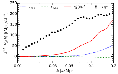
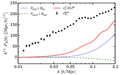
Figure 1: A comparison of the PT correction terms at $z=0$ for $P^{\rm hm}_{\,00}$ (left) and $P^{\rm hm}_{\,01}$ (right). The data points are the nonlinear matter power spectrum directly measured from our simulations described in Sec. III.

II.3 The bispectrum and the bias renormalization

So far we have observed that the four bias parameters, i.e., $(b_{1},b_{2},b_{s^{2}},b_{3\rm nl})$ are introduced to describe the cross power spectrum between halo density and matter density, or the one between halo density and matter momentum at the next-to-leading order when the nonlocal bias terms are considered. As is discussed in Ref. Baldauf et al. (2012), the bispectrum at the lowest order (i.e., at tree level) demands perturbations only up to the second order, described as

$$B^{\rm hmm}_{\,000}(\mbox{\boldmath$k$}_{1},\mbox{\boldmath$k$}_{2},\mbox{\boldmath$k$}_{3})=b_{1}B^{\rm mmm}_{\,000}(\mbox{\boldmath$k$}_{1},\mbox{\boldmath$k$}_{2},\mbox{\boldmath$k$}_{3})+P(k_{1})P(k_{2})\left[b_{2}+b_{s^{2}}\left(\mu_{k_{1},k_{2}}^{2}-\frac{1}{3}\right)\right],$$ (31)

where $\mu_{k_{1},k_{2}}$ is cosine of the angle between $\mbox{\boldmath$k$}_{1}$ and $\mbox{\boldmath$k$}_{2}$, and the three arguments satisfy $\mbox{\boldmath$k$}_{1}+\mbox{\boldmath$k$}_{2}+\mbox{\boldmath$k$}_{3}=0$. In order to derive this as well as Eq. (26) starting from Eq. (55), one may notice that a nontrivial approximation has been introduced, namely, $b_{1}\simeq c_{1}$. However, Ref. McDonald (2006) argued that this is not the case. As we have seen in the renormalization procedure, all the renormalized terms originate from those in the limit of $k\to 0$. This fact means that a physical biased field should be defined so that homogeneous mean density is recovered at $k\to 0$. In other words, we should start with

$$\delta_{\rm h}(\mbox{\boldmath$x$}) = b_{1}\delta_{\rm m}(\mbox{\boldmath$x$})+\frac{1}{2}b_{2}\left[\delta_{\rm m}(\mbox{\boldmath$x$})^{2}-\langle\delta_{\rm m}(\mbox{\boldmath$x$})^{2}\rangle\right]+\frac{1}{2}b_{s^{2}}\left[s(\mbox{\boldmath$x$})^{2}-\langle s(\mbox{\boldmath$x$})^{2}\rangle\right]+\dots,$$ (32)

rather than Eq. (55), and hence Eqs. (26) and (31) are naturally derived. The same argument can be found in Assassi et al. (2014) as well.

Ref. Baldauf et al. (2012) shows that the specific $\mu_{k_{1},k_{2}}$ dependence in Eq. (31) enables us to reliably determine both of the second-order bias parameters, $b_{2}$ and $b_{s^{2}}$ at the same time from the large-scale bispectrum. In later section we are going to simultaneously fit the power spectrum as well as the bispectrum, while Ref. Baldauf et al. (2012) fit the bispectrum with a prior on the linear bias $b_{1}$ determined from the halo-matter power spectrum only at $z=0$. In Appendix B, we present the results when we fit solely to the bispectrum with $b_{1}$ treated as free. In short, the differences in two approaches are generally small especially for $b_{s^{2}}$, indicating that $b_{s^{2}}$ is essentially determined by the characteristic $\mu_{k_{1},k_{2}}$ dependence.

II.4 Coevolution of halos and dark matter up to third order

So far we have discussed what kind of nonlocal bias terms are allowed in terms of symmetry in the fields set by gravity. Another way of studying the nonlocal bias terms induced by nonlinear gravitational evolution is to perturbatively solve the coupled equations between halos and dark matter under fluid approximation. This coevolution picture was first introduced by Fry (1996), followed by e.g., Taruya (2000); Hui and Parfrey (2008); Chuen Chan et al. (2012); Baldauf et al. (2012). Here we simply assume the initial condition is purely local in the Lagrangian space, and thus this simple coevolution approach corresponds to the local Lagrangian evolution model. Assuming no velocity bias and a conservation of halo number, the continuity and the Euler equations combined with the Poisson equation for a matter-halo system are given by

$$\delta_{\rm h}(\mbox{\boldmath$k$},y)^{\prime}-\theta(\mbox{\boldmath$k$},y) = \int\frac{d^{3}q}{(2\pi)^{3}}\alpha(\mbox{\boldmath$q$},\mbox{\boldmath$k$}-\mbox{\boldmath$q$})\theta(\mbox{\boldmath$q$},y)\delta_{\rm h}(\mbox{\boldmath$k$}-\mbox{\boldmath$q$},y),$$ (33)

$$\delta_{\rm m}(\mbox{\boldmath$k$},y)^{\prime}-\theta(\mbox{\boldmath$k$},y) = \int\frac{d^{3}q}{(2\pi)^{3}}\alpha(\mbox{\boldmath$q$},\mbox{\boldmath$k$}-\mbox{\boldmath$q$})\theta(\mbox{\boldmath$q$},y)\delta_{\rm m}(\mbox{\boldmath$k$}-\mbox{\boldmath$q$},y),$$ (34)

$$\{f\theta(\mbox{\boldmath$k$},\eta)\}^{\prime}+\left(1+\frac{\mathcal{H}^{\prime}}{\mathcal{H}^{2}}\right)\theta(\mbox{\boldmath$k$},y)-\frac{3}{2f}\Omega_{\rm m}(y)\delta_{\rm m}(\mbox{\boldmath$k$},y) = f\int\frac{d^{3}q}{(2\pi)^{3}}\beta(\mbox{\boldmath$q$},\mbox{\boldmath$k$}-\mbox{\boldmath$q$})\theta(\mbox{\boldmath$q$},\eta)\theta(\mbox{\boldmath$k$}-\mbox{\boldmath$q$},\eta),$$ (35)

where we introduce $y\equiv\ln D(\eta)$ as a time variable rather than the conformal time $\eta$, and the prime denotes derivative w.r.t $y$. The Hubble parameter $\mathcal{H}$ is defined by $\mathcal{H}=da/(ad\eta)$. The linear-order solutions for this system are give by $\delta^{(1)}_{\rm m}(\mbox{\boldmath$k$},y)=e^{y}\delta_{0}(\mbox{\boldmath$k$},y_{i})$, $\theta^{(1)}(\mbox{\boldmath$k$},y)=\delta^{(1)}(\mbox{\boldmath$k$},y)$, and $\delta^{(1)}_{\rm h}(\mbox{\boldmath$k$},y)=b^{\rm E}_{1}(y)e^{y}\delta_{0}(\mbox{\boldmath$k$},y_{i})$ where

$$\frac{b^{\rm L}_{1}(y)}{b^{\rm L}_{1}(y_{i})}=\frac{b^{\rm E}_{1}(y)-1}{b^{\rm E}_{1}(y_{i})-1}=\frac{e^{y_{i}}}{e^{y}}.$$ (36)

As is shown in Ref. Catelan et al. (1998); Baldauf et al. (2012); Chuen Chan et al. (2012), the second-order solution for halos is written by

$$\delta^{(2)}_{\rm h}(\mbox{\boldmath$k$},y) = b^{\rm E}_{1}(y)\int\frac{d^{3}q}{(2\pi)^{3}}F^{(2)}_{\rm S}(\mbox{\boldmath$q$},\mbox{\boldmath$k$}-\mbox{\boldmath$q$})\delta^{(1)}_{\rm m}(\mbox{\boldmath$q$},y)\delta^{(1)}_{\rm m}(\mbox{\boldmath$k$}-\mbox{\boldmath$q$},y)$$ (37)

$$\ +\left\{\frac{1}{2}b^{\rm L}_{2}(y)+\frac{4}{21}b^{\rm L}_{1}(y)\right\}\int\frac{d^{3}q}{(2\pi)^{3}}\delta^{(1)}_{\rm m}(\mbox{\boldmath$q$},\eta)\delta^{(1)}_{\rm m}(\mbox{\boldmath$k$}-\mbox{\boldmath$q$},y)$$

$$\ -\frac{2}{7}b^{\rm L}_{1}(y)\int\frac{d^{3}q}{(2\pi)^{3}}S^{(2)}(\mbox{\boldmath$q$},\mbox{\boldmath$k$}-\mbox{\boldmath$q$})\delta^{(1)}_{\rm m}(\mbox{\boldmath$q$},y)\delta^{(1)}_{\rm m}(\mbox{\boldmath$k$}-\mbox{\boldmath$q$},y),$$

where we used the fact that $b_{n}^{\rm L}(y)=b_{n}^{\rm L}(y_{i})e^{n(y-y_{i})}$. Hence a correspondence of the local and nonlocal bias terms at second order to Eq. (59) is clearly found, and it shows that the tidal field is allowed to be a source of the nonlocal bias at second order:

$$b^{\rm coev}_{2} = b^{\rm L}_{2}(y)+\frac{8}{21}b^{\rm L}_{1}(y),$$ (38)

$$b^{\rm coev}_{s^{2}} = -\frac{4}{7}b^{\rm L}_{1}(y)=-\frac{4}{7}(b^{\rm E}_{1}(y)-1).$$ (39)

Continuing to this exercise to third order, we find the solution as

$$\delta^{(3)}_{\rm h}(\mbox{\boldmath$k$},y) = \delta^{(3)}_{\rm h}(\mbox{\boldmath$k$},y_{i})+\frac{1}{3}\int\frac{d^{3}q_{1}}{(2\pi)^{3}}\frac{d^{3}q_{2}}{(2\pi)^{3}}G^{(3)}_{\rm S}(\mbox{\boldmath$q$}_{1},\mbox{\boldmath$q$}_{2},\mbox{\boldmath$k$}-\mbox{\boldmath$q$}_{1}-\mbox{\boldmath$q$}_{2})\,\delta^{(1)}_{\rm m}(\mbox{\boldmath$q$}_{1},y)\delta^{(1)}_{\rm m}(\mbox{\boldmath$q$}_{2},y)\delta^{(1)}_{\rm m}(\mbox{\boldmath$k$}-\mbox{\boldmath$q$}_{1}-\mbox{\boldmath$q$}_{2},y)$$ (40)

$$\ +\left(\frac{1}{2}b_{1}^{\rm L}(y)+\frac{1}{3}\right)\int\frac{d^{3}q_{1}}{(2\pi)^{3}}\frac{d^{3}q_{2}}{(2\pi)^{3}}\left[\alpha(\mbox{\boldmath$q$}_{1},\mbox{\boldmath$q$}_{2}+\mbox{\boldmath$q$}_{3})F^{(2)}_{\rm S}(\mbox{\boldmath$q$}_{2},\mbox{\boldmath$q$}_{3})\right]_{\rm sym}\,\delta^{3}$$

$$\ +\left[\frac{1}{2}b^{\rm L}_{2}(y)+\frac{2}{21}b^{\rm L}_{1}(y)\right]\int\frac{d^{3}q_{1}}{(2\pi)^{3}}\frac{d^{3}q_{2}}{(2\pi)^{3}}\left[\alpha(\mbox{\boldmath$q$}_{1},\mbox{\boldmath$q$}_{2}+\mbox{\boldmath$q$}_{3})\right]_{\rm sym}\,\delta^{3}$$

$$\ -\frac{1}{4}b_{s^{2}}\int\frac{d^{3}q_{1}}{(2\pi)^{3}}\frac{d^{3}q_{2}}{(2\pi)^{3}}\left[\alpha(\mbox{\boldmath$q$}_{1},\mbox{\boldmath$q$}_{2}+\mbox{\boldmath$q$}_{3})S^{(2)}(\mbox{\boldmath$q$}_{2},\mbox{\boldmath$q$}_{3})\right]_{\rm sym}\,\delta^{3}$$

$$\ +\left(\frac{1}{2}b_{1}^{\rm L}(y)+\frac{1}{3}\right)\int\frac{d^{3}q_{1}}{(2\pi)^{3}}\frac{d^{3}q_{2}}{(2\pi)^{3}}\left[\alpha(\mbox{\boldmath$q$}_{2}+\mbox{\boldmath$q$}_{3},\mbox{\boldmath$q$}_{1})G^{(2)}_{\rm S}(\mbox{\boldmath$q$}_{2},\mbox{\boldmath$q$}_{3})\right]_{\rm sym}\,\delta^{3}.$$

Although the third-order solution looks somewhat complicated, it is useful to isolate its contribution to the matter-halo power spectrum, i.e., $\langle\delta^{(3)}_{\rm h}(\mbox{\boldmath$k$},y)\delta^{(1)}_{\rm m}(\mbox{\boldmath$k$},y)\rangle$. Subtracting out the terms proportional to the linear bias, we find

$$P^{\rm hm,(31)}_{\rm coev}(k)-b^{\rm E}_{1}P^{(31)}(k)=\frac{32}{315}b^{\rm L}_{1}\sigma^{2}_{3}P(k)+\left(b^{\rm L}_{2}+\frac{1}{2}b^{\rm L}_{3}\right)\sigma^{2}P(k).$$ (41)

Now it is straightforward to correspond this formula to Eq. (12):

$$b^{\rm coev}_{3{\rm nl}} = \frac{32}{315}b^{\rm L}_{1}(y)=\frac{32}{315}(b^{\rm E}_{1}(y)-1),$$ (42)

$$b_{1} = b_{1}^{\rm E}+\left(b^{\rm L}_{2}+\frac{1}{2}b^{\rm L}_{3}\right)\sigma^{2}.$$ (43)

Thus the nonlocal bias term at third order which we discussed in the previous section can be related to the linear Lagrangian bias in this specific way. We will compare this prediction with our $b_{\rm 3nl}$ measurement from simulations in the following sections.

III $N$-body simulations and the fitting methodology

III.1 $N$-body simulation detail

We performed a suite of $N$-body simulations using the publicly available Gadget2 code Springel (2005) to make 14 realizations at $z=0$, $0.5$ and $1$ with cosmological parameters in a flat $\Lambda$CDM model preferred by the WMAP results Komatsu et al. (2009), i.e., a mass density parameter $\Omega_{\rm m}=0.272$, a baryon density parameter $\Omega_{\rm b}=0.0455$, a Hubble constant $h=0.704$, a spectral index $n_{\rm s}=0.967$, and a normalization of the curvature perturbations of $\Delta^{2}_{\mathcal{R}}=2.42\times 10^{-9}$ at the pivot scale of $k=0.002\,{\rm Mpc}^{-1}$, giving $\sigma_{8}=0.81$. The total simulation volume is $47.25\,[({\rm Gpc}/h)^{3}]$ which is larger roughly by a factor of ten than the current galaxy survey like BOSS. We generated initial conditions at $z=99$ using the second-order Lagrangian perturbation theory to initialize the second order growth correctly and allow for a reliable bispectrum extraction at low redshift. The box size and number of particles are $L=1500\,{\rm Mpc}/h$ and $N_{\rm particle}=1024^{3}$, respectively, yielding a particle mass resolution of $2.37\times 10^{11}\,M_{\odot}/h$.

We identify halos using the Friends-of-Friends finder with a linking length of 0.2 times the mean inter particle spacing. We only take halos which contain more than 20 particles, and hence our minimum halo mass is approximately $4.74\times 10^{12}\,M_{\odot}/h$. We divide the halo catalog into several mass bins at each redshift slice, whose detail is summarized in Table. 1. Note that $\sim 10^{13}M_{\odot}/h$ halo roughly corresponds to a typical host halo in which observed galaxies live. In order to estimate the power spectrum and the bispectrum, the particles are assigned on a $N_{\rm c}=1024$ grid with the Cloud-in-Cell algorithm, and the gridded density field is properly corrected by the window function. We also estimate the power spectrum of mass-weighted momentum of matter, following the method in Okumura et al. (2012a, b). Note that our simulation is different from that used in Desjacques et al. (2009); Baldauf et al. (2012); Okumura et al. (2012a, b). We mainly focus on combined measurement using the power spectrum and the bispectrum but will present results in the case of the bispectrum only in Appendix B.

The errors of the power spectrum are estimated by the standard deviation among 14 realizations. Strictly speaking, it might be necessary to evaluate the covariance matrix to take account for the off-diagonal correlation among different modes. However, we neglect the correlation between different modes, since we focus on somewhat large scales, $k\raisebox{-2.15277pt}{$\>\stackrel{{\scriptstyle\textstyle<}}{{\sim}}\>$}0.1\,h/{\rm Mpc}$. This part can be definitely improved by a proper treatment of the covariance matrix with larger number of realizations.

redshift	mass bin	$\overline{M}_{\rm halo}\,[10^{13}\,M_{\odot}/h]$	$b_{1}$	$b_{2}$	$b_{s^{2}}$	$b_{3\rm nl}$
1	I	0.763	$2.0419\pm 0.0089$	$-0.168\pm 0.027$	$-1.099\pm 0.064$	$0.211\pm 0.074$
	II	2.24	$2.7957\pm 0.0114$	$1.766\pm 0.039$	$-1.409\pm 0.094$	$0.133\pm 0.100$
	III	6.50	$4.0294\pm 0.0170$	$8.0362\pm 0.062$	$-1.708\pm 0.165$	$0.245\pm 0.150$
0.5	I	0.769	$1.4426\pm 0.0057$	$-0.792\pm 0.018$	$-0.469\pm 0.038$	$0.153\pm 0.030$
	II	2.29	$1.9033\pm 0.0078$	$-0.394\pm 0.024$	$-0.785\pm 0.052$	$0.170\pm 0.043$
	III	6.75	$2.7005\pm 0.0115$	$1.586\pm 0.035$	$-1.286\pm 0.080$	$0.268\pm 0.061$
	IV	19.3	$4.1349\pm 0.0204$	$8.650\pm 0.066$	$-1.837\pm 0.155$	$-0.294\pm 0.112$
0	I	0.773	$1.0488\pm 0.0048$	$-0.777\pm 0.013$	$-0.099\pm 0.026$	$0.092\pm 0.019$
	II	2.33	$1.3094\pm 0.0062$	$-0.873\pm 0.018$	$-0.267\pm 0.035$	$0.132\pm 0.023$
	III	6.92	$1.7977\pm 0.0087$	$-0.462\pm 0.025$	$-0.514\pm 0.051$	$0.193\pm 0.035$
	IV	20.1	$2.6741\pm 0.0136$	$1.500\pm 0.040$	$-1.028\pm 0.086$	$0.105\pm 0.053$

Table 1: Summary of halo catalogs used in this paper. We also show the best-fitting values of four bias parameters determined by our fitting from the power spectrum and the bispectrum. The fitting range, $k_{\rm max}$, depends on redshift (see text on how to choose $k_{\rm max}$ in detail): $(k_{{\rm max},P(k)},k_{{\rm max},B(k)})=(0.08,0.065)$, $(0.10,0.075)$, and $(0.125,0.075)$ at $z=0$, $0.5$ and $1$, respectively. Note that the definition of second-order bias parameters in Baldauf et al. (2012) differs by a factor of two.

III.2 Fitting procedure

Let us briefly summarize how we determine the bias parameters from the simulated power spectra. As explained in the previous section, we have four bias parameters as free, i.e., two local bias parameters, $b_{1}$ and $b_{2}$, and second- and third-order nonlocal bias ones, $b_{s^{2}}$ and $b_{3\rm nl}$. When we fit the bias model to the halo-matter density power spectrum only, the fitted bias parameters are estimated so that they minimize

$$\chi^{2}_{P00}=\sum_{k_{i}\leq k_{{\rm max},P(k)}}\frac{\left[P^{\rm hm}_{\,00}(k_{i})-\hat{P}^{\rm hm}_{\,00}(k_{i})\right]^{2}}{\Delta P^{\rm hm}_{\,00}(k_{i})^{2}}.$$ (44)

Here theoretical template of $P^{\rm hm}_{\,00}$ at $k=k_{i}$ is given by Eq. (12), $\hat{P}^{\rm hm}_{\,00}$ denotes the spectrum measured from the simulations, $\Delta P^{\rm hm}_{\,00}$ denotes the error of the spectrum amplitude, and $k_{{\rm max},P(k)}$ is the maximum wavenumber in the power spectrum analysis. Likewise we apply exactly the same procedure for the cross power spectrum between halo-density and matter-momentum by replacing ‘00’ with ‘01’ in the subscript in Eq. (44). Note that we always insert the measured spectra from the simulation for nonlinear matter part, $P^{\rm NL}_{\delta\delta}$ for $P^{\rm mm}_{\,00}$ and $\{P^{\rm NL}_{\delta\theta}+B_{b1}\}$ for $P^{\rm mm}_{\,01}$. We also note that we use the power spectra averaged over 14 realizations rather than one in each realization. This is the reason why we will observe somewhat low values of reduced $\chi^{2}$, and hence this is not an overfitting issue. When we quote ‘00 only’ (‘01 only’), we simply use $\chi^{2}_{P(k)}=\chi^{2}_{P00}$ ($\chi^{2}_{P(k)}=\chi^{2}_{P01}$). When we include both $P^{\rm hm}_{\,00}$ and $P^{\rm hm}_{\,01}$, we assume they are independent and simply add two $\chi^{2}$ by neglecting the correlation between two, i.e., $\chi^{2}_{P(k)}=\chi^{2}_{P00}+\chi^{2}_{P01}$. In principle, we could estimate the covariance matrix which includes correlation between both signals but the number of our realizations would not be sufficient to properly estimate it (see e.g. Percival et al. (2013) for a recent study in such a direction).

The similar procedure is adopted for the bispectrum as well. We search the best-fitting values of the bias parameters for the bispectrum so that they minimize

$$\chi^{2}_{B(k)}=\sum_{k_{i,j}\leq k_{{\rm max},B(k)}}\frac{\left[B^{\rm hmm}_{\,000}(k_{i},k_{j},\mu_{ij})-\hat{B}^{\rm hmm}_{\,000}(k_{i},k_{j},\mu_{ij})\right]^{2}}{\Delta B^{\rm hmm}_{\,000}(k_{i},k_{j},\mu_{ij})^{2}},$$ (45)

where $\mu_{i,j}$ is the cosine between $\mbox{\boldmath$k$}_{1}$ and $\mbox{\boldmath$k$}_{2}$, the theoretical template of $B^{\rm hmm}_{\,000}$ is given by Eq. (31), $\Delta B^{\rm hm}_{\,00}$ denotes the error of the bispectrum amplitude, and $k_{{\rm max},B(k)}$ is the maximum wavenumber in the bispectrum analysis. Notice that the bispectrum depends only on three bias parameters, $b_{1}$, $b_{2}$ and $b_{s^{2}}$. We distinguish the maximum wavenumber range in the power spectrum case from that in the bispectrum. It is not entirely clear if higher-order PT terms for different statistics become dominant at the same wavenumber. Our main purpose is to investigate how large the their-order contribution is, and hence we fix $k_{{\rm max},B(k)}$ to 0.065 (0.075)$h/$Mpc at $z=0$ ($z=0.5$ or $1$) in the following analysis. These choices are based on our fitting results to the bispectrum only, presented in Appendix B. Thus, we adopt $\chi^{2}=\chi^{2}_{P(k)}+\chi^{2}_{B(k)}$ when we jointly fit the PT model to the power spectrum and the bispectrum.

In order to fully investigate the probability distribution of preferred values of the bias parameters, we adopt the Markov chain Monte Carlo (MCMC) technique, assuming the Gaussian likelihood, i.e., $\mathcal{L}\propto\exp(-\chi^{2}/2)$. For this end, we modify the COSMOMC code Lewis and Bridle (2002), considering future applications of the code to the actual galaxy sample. We ensure convergence of each chain, imposing $R<0.003$ where $R$ is the standard Gelman-Rubin criteria.

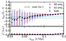
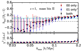
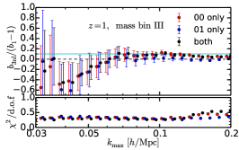
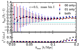
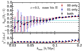
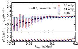
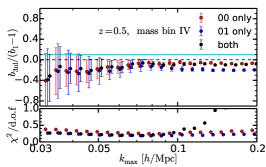
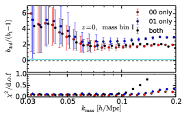
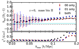
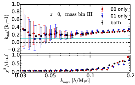
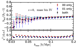
Figure 2: The best-fitting values of $b_{3{\rm nl}}$ as a function of $k_{\rm max}$. We present results at $z=1$ (top three), at $z=0.5$ (middle four), and at $z=0$ (bottom four), for light to heavy (from I to IV) halo mass bins. In each panel, we show results in the case of $P^{\rm hm}_{\,00}$ only (red), $P^{\rm hm}_{\,01}$ only (blue), and both of two (black). The goodness of fit, $\chi^{2}_{P(k)}/{\rm d.o.f}$, is also plotted in the lower part of each panel. Note that we jointly fit the bispectrum together with the power spectrum. For comparison, the prediction from the coevolution picture (local Lagrangian bias model), $32/315$, is indicated by the horizontal line (cyan solid).

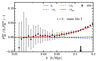
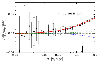
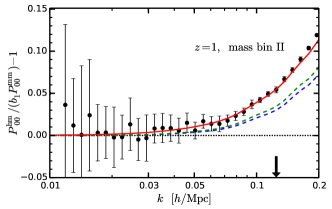
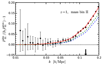
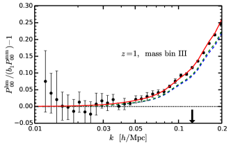
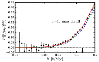
Figure 3: The power spectra with best-fitting bias parameters at $z=1$. We here plot $P^{\rm hm}_{X}(k)/(b_{1}P^{\rm mm}_{X}(k))-1$ where $X$ is ‘00’ (left) or ‘01’ (right) with the best-fitting values of $b_{1}$ and $b_{\rm 3nl}$ at $k_{\rm max}=0.125\,h$/Mpc (specified as an arrow). Namely, zero values (black dotted) mean it matches to the linear bias term, any deviation from zero represents deviation from the linear bias model. The red solid line corresponds to the case including all contributions. The blue dashed line includes only local bias terms up to second order, while the green dashed line includes local and nonlocal bias terms up to second order.

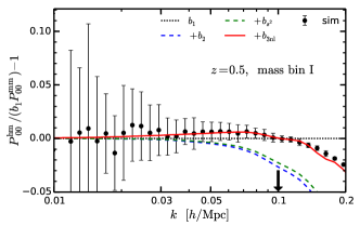
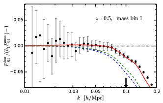
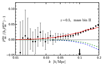
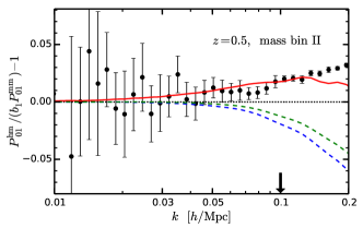
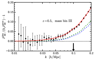
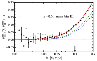
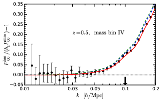
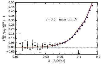
Figure 4: Same as Fig. 3, but at $z=0.5$. The best-fitting values are derived at $k_{\rm max}=0.1\,h$/Mpc (specified as an arrow).

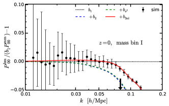
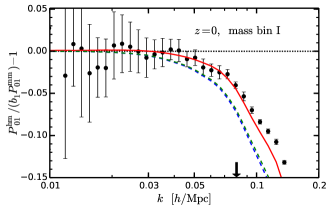
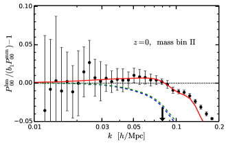
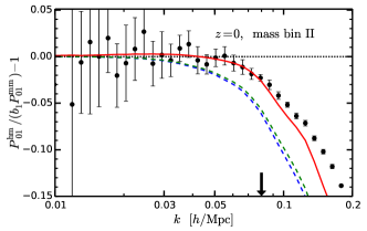
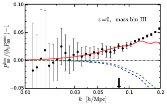
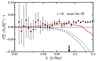
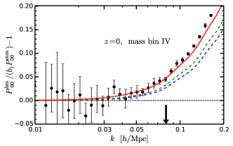
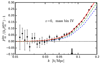
Figure 5: Same as Fig. 3, but at $z=0$. The best-fitting values are derived at $k_{\rm max}=0.08\,h$/Mpc (specified as an arrow).

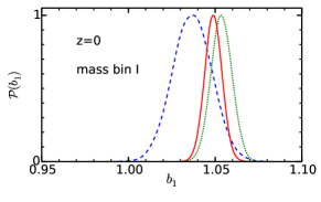
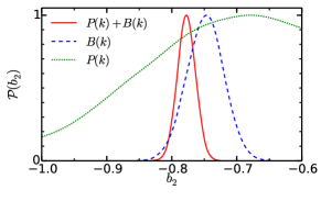
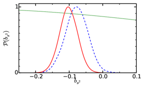
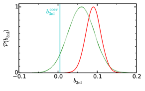
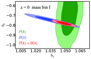
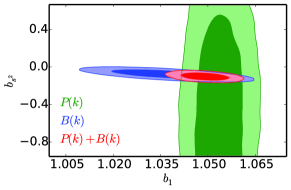
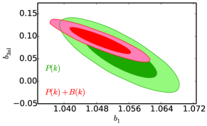
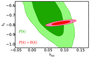
Figure 6: (Upper four panels) comparison between cases with and without combining the bispectrum information for mass bin I at $z=0$. We show the marginalized probability distribution for each bias parameter in the cases of the power spectrum combined with the bispectrum (red solid), the bispectrum only (blue dashed), and the power spectrum only (green dotted). As a reference, we show the prediction from the coevolution $b^{\rm coev}_{\rm 3nl}$ assuming $b_{1}\simeq b^{\rm E}_{1}$ is equal to the value obtained by joint fitting (cyan). Note that, in the case of the power spectrum, we use both density-density and density-momentum power spectrum with $k_{{\rm max},P(k)}=0.08h$/Mpc. (Lower four panels) the marginalized two-dimensional contours (68% and 95% C.L.) among the nonlinear bias parameters.

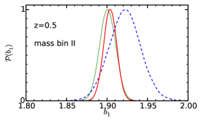
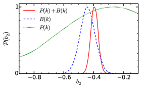
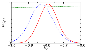
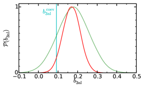
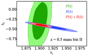
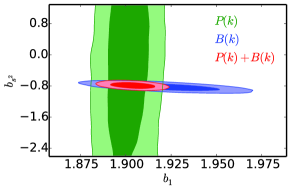
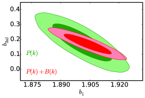
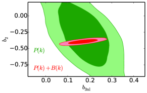
Figure 7: Same as Fig. 6, but for mass bin II at $z=0.5$. Note that, in the case of the power spectrum, we use both density-density and density-momentum power spectrum with $k_{{\rm max},P(k)}=0.1h$/Mpc.

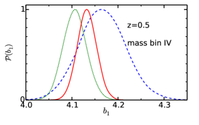
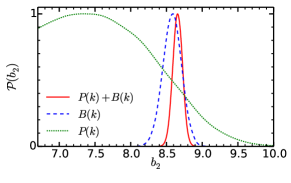
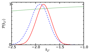
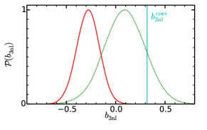
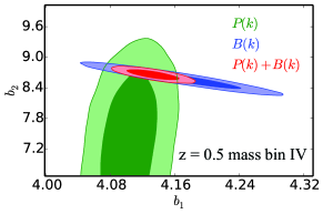
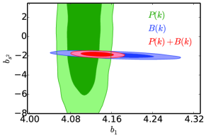
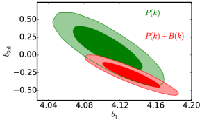
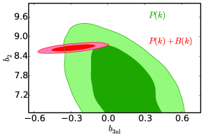
Figure 8: Same as Fig. 6, but for mass bin IV at $z=0.5$. Note that, in the case of the power spectrum, we use both density-density and density-momentum power spectrum with $k_{{\rm max},P(k)}=0.1h$/Mpc.

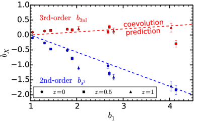
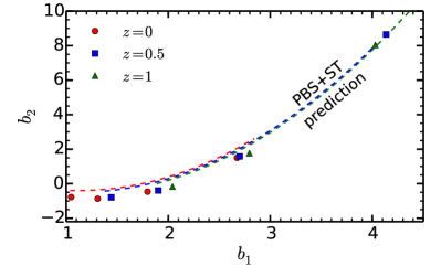
Figure 9: (Left) nonlocal bias values at second and third orders as a function of the linear bias parameter. Each point is taken from the result in the joint fit of the power spectrum and the bispectrum. Both of them are compared with the values expected from the local Lagrangian bias in the simple convolution picture (dashed lines). (Right) second-order local bias bias $b_{2}$ against $b_{1}$. Again each point is obtained from our joint fit. For comparison, we draw theory lines which is based on the peak-background split with the universal mass function (see text in detail). Note that the range of these lines are limited since we here consider relevant halo mass range only ($0.6\raisebox{-2.15277pt}{$\>\stackrel{{\scriptstyle\textstyle<}}{{\sim}}\>$}M_{\rm halo}\,[10^{13}M_{\odot}/h]\raisebox{-2.15277pt}{$\>\stackrel{{\scriptstyle\textstyle<}}{{\sim}}\>$}21$).

IV Results

Now we show our measurements of the bias parameters from the simulated halo-matter power spectra combined together with the bispectrum. In Fig. 2, we show the best-fitting values of $b_{3{\rm nl}}$ as a function of $k_{\rm max}$ for each mass bin at each redshift. First of all, the preferred values of $b_{3{\rm nl}}$ are nonzero generally for any halo mass bin at any redshift, at $k_{\rm max}\sim 0.1\,h/{\rm Mpc}$. Also, the best-fitting values of $b_{3{\rm nl}}$ from $P^{\rm hm}_{\,00}(k)$ are generally in a good agreement with those from $P^{\rm hm}_{\,01}(k)$, indicating that the third-order nonlocal bias term is important to explain both $P^{\rm hm}_{\,00}(k)$ and $P^{\rm hm}_{\,01}(k)$. If looking at smaller scales at $k\raisebox{-2.15277pt}{$\>\stackrel{{\scriptstyle\textstyle>}}{{\sim}}\>$}0.1\,h/{\rm Mpc}$, we start to see a discrepancy between the two results, and the best-fitting values tend to vary as a function of $k_{\rm max}$. In addition, a goodness of fit, $\chi^{2}$/(d.o.f.) becomes worse at larger $k$. This clearly shows that our bias model fails to describe the halo-matter power spectra at such small scales, and higher-order contribution would start to kick in. Notice again that our values of the goodness of fit is somewhat small ($\mathcal{O}(0.1)$) simply because we adopt the nonlinear matter power spectra taken from the simulation itself, and we do not worry about unrealistic overfitting issues here. Since our $b_{3\rm nl}$ measurements look convergent up to a certain $k_{\rm max}$ but start to vary at larger $k_{\rm max}$, it is difficult to define the reliable range of the bias model which could depends on both redshift and halo mass. We here simply and conservatively quote the measured values of $b_{3{\rm nl}}$ at $k_{\rm max}=0.08,\,0.1$, and 0.125 at $z=0,\,0.5$, and 1, respectively, which roughly correspond to valid range of the standard perturbation theory Carlson et al. (2009); Nishimichi et al. (2009).

We quantify contribution of the third-order nonlocal bias term to each power spectrum in Figs. 3, 4, and 5 for $z=1$, 0.5 and 0, respectively. We plot $P^{\rm hm}_{X}(k)/(b_{1}P^{\rm mm}_{X}(k))-1$ with $X$ being ‘00’ or ‘01’, which manifests deviation from the linear bias term. The blue lines show the nonlinear contributions from local term only, i.e., the $b_{2}$ term, while the green lines show ones from second-order local plus nonlocal terms, i.e., the $b_{2}$ term plus the $b_{s^{2}}$ one. Our best-fitting results including the third-order nonlocal bias term is shown by the red curves. Clearly seen from the figures, the local bias model cannot explain the simulated halo-matter spectra, and even including second-order nonlocal bias terms does not drastically help in general. Meanwhile, adding the third-order nonlocal bias term can apparently explain the power spectra very well. Within the valid range, the fractional differences between the simulated and fitted spectra are typically at a few percent level. This result is already expected from the behavior of the PT terms in Fig. 1. The reason why we obtain negative values of $b_{\rm 3nl}$ at mass bin IV at $z=0.5$ is obvious from the figures. At these bins, the bispectrum prefers large second-order bias parameters, especially $b_{2}$, whose contribution exceed the measured halo-matter power spectra. Therefore the negative $b_{\rm 3nl}$ is necessary to compensate with the second-order terms.

Given the fact that the contribution of the second-order terms are generally lower than that of the third-order nonlocal term, it is interesting to see to what extent we can simultaneously constrain four bias parameters only from the power spectra, i.e., without help of information on the second-order bias parameters from the bispectrum. We often encounter a similar situation in analyzing the actual galaxy survey if we only have the power spectrum measurement available, although we focus on the unobservable halo-matter power spectra throughout this work. Also, it is interesting to separate the information of the power spectrum out of that of the bispectrum and to understand the parameter degeneracy in the PT model. Figs. 6-8 show 1D and 2D marginalized posterior distribution for constraints on the bias parameters. Generally speaking, the third-order nonlocal bias $b_{3\rm nl}$ is well constrained even only from the power spectra, while the second-order bias parameters cannot be tightly constrained only by the power spectra (green). The second-order nonlocal bias, $b_{s^{2}}$ cannot be constrained at all by the power spectra, since the amplitude of the $b_{s^{2}}$ term in the power spectra is fairly small compared to other terms as seen in Fig. 1. The second-order local bias $b_{2}$ can be constrained by the power spectra, but we confirm that the bispectrum is more sensitive to $b_{2}$. At low and intermediate mass bins (see Figs. 6 and 7), the preferred values of $b_{2}$ both from the power spectra and the bispectrum are consistent with each other, and hence the resultant values of $b_{\rm 3nl}$ in both cases of $P(k)$ and of $P(k)+B(k)$ become consistent as well. At massive bin (see Fig. 8), this story seems a bit different. Since the preferred values of $b_{1}$ and $b_{2}$ from the bispectrum at at mass bin IV of $z=0.5$ are larger than those from the power spectra, the well-fitting $b_{\rm 3nl}$ from the combined case becomes lower than the one only from the power spectrum. Equivalently, the $b_{\rm 3nl}$ term become less important at higher mass bins, and the $b_{2}$ terms become dominant over the $b_{\rm 3nl}$ term. Furthermore, the linear bias value can be constrained solely by the bispectrum and its agreement with the power spectrum-only result becomes worse for more massive halos. The constraining power of the power spectrum on $b_{1}$ is weaker than what can be found in the literature. This is a consequence of an anti-correlation between $b_{1}$ and $b_{\rm 3nl}$. This fact implies that the $b_{\rm 3nl}$ term becomes important at fairly large scales, $k\raisebox{-2.15277pt}{$\>\stackrel{{\scriptstyle\textstyle<}}{{\sim}}\>$}0.1\,h$/Mpc and has a non-negligible impact on determination of the linear bias value. We here do not investigate how these correlations affect estimation of cosmological parameters of interest and will be addressed in future work.

Finally, we make a comparison between our $b_{3{\rm nl}}$ measurements with a theoretical prediction in order to make sure if our results are physically expected. For this purpose, we compare our results with the prediction, Eq. (42), in the simple coevolution picture (or the local Lagrangian bias) as discussed in §. II.4. The cyan horizontal (vertical) line in each panel of Fig. 2 (Figs. 6-8) is already drawn, and the left panel of Fig. 9 summarizes such a comparison which includes both second- and third-order nonlocal bias parameters as a function of the linear bias $b_{1}$. Notice that it is not clear if our measured $b_{1}$ truly corresponds to $b_{1}^{\rm E}$ (see Eq. (43)) but we here simply assume $b_{1}\simeq b_{1}^{\rm E}$ for simplicity. As clearly seen in Fig. 9, overall agreement in third-order nonlocal bias is as good as that in second-order, although the agreement is apparently not perfect. Also, the $b_{\rm 3nl}$ value at mass bin IV of $z=0.5$ exceptionally deviates from the coevolution prediction. As we discussed above, however, the value preferred from the power spectrum only is more consistent with the coevolution prediction (see green dotted line in Fig.8). Again, this difference comes from the fact that the mass bin IV of $z=0.5$ prefers larger $b_{2}$ which more affects the power spectrum and the bispectrum than the nonlocal bias terms. There are several sources which could make the prediction different from the local Lagrangian bias as we will discuss in the following section. However, it is worth mentioning that our $b_{\rm 3nl}$ measurement is not far from the coevolution prediction which is one of the simplest physical models one thinks of. This fact also implies an evidence of the third-order nonlocal bias term. In the right panel of Fig. 9, we also compare our measurements of the second-order local bias $b_{2}$ from the joint fit with theoretical prediction that is based on the peak-background split (PBS) with the universal mass function (see Appendix. D in detail). Clearly seen from the figure, the measured $b_{2}$ values are systematically lower than the theoretical predictions at fixed $b_{1}$, while the characteristic dependence on $b_{1}$ is qualitatively similar. Note that it is a coincidence that two points around $b_{1}\sim 4$ look in a perfect agreement with the prediction, since they deviate from predictions in $(b_{1},M_{\rm halo})$ or $(b_{2},M_{\rm halo})$ plane.

V Summary and discussion

The nonlocality of halo bias is naturally induced by nonlinear gravitational evolution as suggested by recent studies. In this paper we study how well the PT model including nonlocal bias effects perform against the halo statistics simulated in $N$-body simulations in a $\Lambda$CDM universe. For this purpose we first revisit the bias renormalization scheme proposed by McDonald and Roy (2009) and show that, while the leading-order bispectrum requires only one second-order nonlocal bias term, $b_{s^{2}}$ (see Eq. (31)), the power spectrum at next-to-leading order demands an additional nonlocal bias term, $b_{\rm 3nl}$, associated with the third-order perturbation (see Eq. (12)). We extend this model to the power spectrum between halo density and matter momentum, and show that there is an exactly same correction of the $b_{\rm 3nl}$ term in this case as well (see Eq. (30)). The fact that we only need one additional nonlocal bias even at third order may sound surprising. However, we argue that this is actually expected since the symmetry in gravity basically restricts the allowed functional form of nonlocal terms. In order to confirm this, we show that the PT kernel in the $b_{3\rm nl}$ term exactly matches to the solution in a simple coevolution picture between dark matter and halo fluids (see discussion in §. II.4). Also, this circumstance evidence becomes even much clearer when the solution in coevolution picture is found out to be consistent with that derived by the Galileon invariants (see Appendix C and similar discussions can be found in Chuen Chan et al. (2012)). Also we note that Ref. Assassi et al. (2014) readdress the bias renormalization in terms of the Effective Field Theory (EFT) language and drew the same conclusion.

Then an inevitable question is whether the model can really well describe the halo statistics in $N$-body simulations. In particular, can the model simultaneously explain the halo power spectrum and the bispectrum which is never achieved in a simple local bias model Pollack et al. (2012, 2013)? To answer this question, we fit the model including nonlocal bias terms to the power spectrum, combined with the bispectrum. We here focus on the cross spectra between halos and dark matter which are free from issues such as halo exclusion Baldauf et al. (2013) or stochasticity Desjacques and Sheth (2010); Hamaus:2012mz; Sato and Matsubara (2013). A novel thing in this work is to compare the model for the cross spectrum between halo density and matter momentum. The momentum power spectrum is the essential ingredient in predicting RSD in the so-called Distribution Function approach as initiated by Seljak and McDonald (2011). We show that the fitting values of $b_{3\rm nl}$ up to a certain $k_{\rm max}$ (typically, $k_{\rm max}\raisebox{-2.15277pt}{$\>\stackrel{{\scriptstyle\textstyle<}}{{\sim}}\>$}0.1h/$Mpc) are in a good agreement for two power spectra, saying that the model seems to be able to explain the power spectra and the bispectrum at the same time. We also explore if the derived values of $b_{3\rm nl}$ are consistent with predictions from the simple coevolution picture (or the local Lagrangian bias) and find as a good agreement as second order tidal bias, $b_{s^{2}}$, although the agreement is not perfect.

Our study does indicate that there is no reason to ignore the nonlocal bias terms in predicting the halo statistics at a high accuracy. In fact there have been some evidences which suggests the third-order nonlocal bias term should be included in the literature. For instance, Refs. Blazek et al. (2013); Vlah et al. (2013) find that they need to introduce two different second-order bias parameters for the halo density-density, $b_{2}^{00}$ and for the halo density-momentum, $b_{2}^{01}$ to explain the simulated halo power spectrum. As is already discussed in Vlah et al. (2013), the difference can be, at least qualitatively, explained by the $b_{3\rm nl}$ term. However, we need to be more careful to analyze the halo-halo statistics by properly taking stochasticity noise and velocity bias into account. Even though many improvements still need to be considered, Ref. Beutler et al. (2013) apply the model based on our study with nonlocal bias values fixed to be the coevolution predisctions to the actual galaxy survey data. One of the reasons why it seems to work is that the authors primarily focus on the anisotropic clustering signal to extract RSD which has larger statistical errors (typically $\sim 10\%$) than the isotropic part (i.e., monopole, typically a few %). Also, additional bias parameters such as the second-order local bias, $b_{2}$, and shot-noise like bias, $N$, are conservatively treated as free. In order to extract the shape information from the monopole, however, more refined analysis will be required. We leave it as our future work and hope to report it elsewhere in the near future. Also, there are extensions of the model considered here, which could make the fit and the comparisons better and extend to higher wavenumbers. Let us summarize the key assumptions of our simple coevolution picture again: local Lagrangian initial conditions, a continuity equation for the halo fluid, and no velocity bias. The local Lagrangian initial conditions will be likely to be modified by the presence of initial $b_{s^{2}}$ and $b_{\rm 3nl}$ due to e.g. ellipsoidal collapse Sheth et al. (2013). Since we are fitting for the amplitude of these terms, our inferred values are a combination of the initial and dynamical contributions and the agreement with the $b_{s^{2}}$, $b_{\rm 3nl}\propto(b_{1}-1)$ scaling tells us that the initial contributions are expected be fairly small. Furthermore, the peak model Bardeen et al. (1986) and studies of proto-haloes in $N$-body simulations Elia et al. (2012) suggest that there is an initial scale dependent linear bias $b_{1}(k)$, which arises from the dependence of the peak clustering on second derivatives of the field (see Desjacques (2008); Schmidt et al. (2012) for a rigorous derivation, and also see Desjacques et al. (2010); Matsubara (2011) for subsequent gravitational evolution taken into account). The same calculation also reveals that proto-halo velocities are likely statistically biased on small scales with respect to the underlying matter. Simple considerations for the motions of peaks suggest that these effects are damped by gravitational evolution at linear level. In absence of a well tested description of these effects at the non-linear level, we refrain from taking these effects into account.

Let us make a comment on a related work in Ref. Biagetti et al. (2014). The authors in Ref. Biagetti et al. (2014) predict the halo-matter power spectrum by fixing bias parameters: the local bias parameters, $b_{1}$ and $b_{2}$, are calculated by the peak-background split combined with the non-universal mass function in the excursion set peak formalism Musso et al. (2012); Paranjape et al. (2013a, b), and the nonlocal bias parameters are fixed with the results of the local Lagrangian bias (i.e., the same as our §. II.4). In addition, a crucial difference is that they include $k^{2}$-type bias term based on the peak formalism. They claim that their predictions are in a good agreement with simulations including cosmology with massive neutrinos Villaescusa-Navarro et al. (2014) at a few percent level, and the $k^{2}$-type term, which we ignored, is important. This sounds contradictory to our results, but we argue it is not actually the case: in Fig. 9, we observe that our preferred $b_{\rm 3nl}$ values are sometimes larger than the coevolution prediction. This means that it is necessary to introduce another component (like $k^{2}$ term) to well fit to the simulated data, if the $b_{\rm 3nl}$ is fixed to the coevolution prediction. In addition, as is already pointed out in Baldauf et al. (2012) and is shown in Fig. 9, the preferred values of the second-order bias, $b_{2}$ and $b_{s^{2}}$, are not in a perfect agreement with the simple theoretical predictions. It is interesting to clarify whether the source of this discrepancy comes truly from the $k^{2}$ bias or something different, which would require more careful investigation.

As a final remark, we make a comment on future directions of our study. As shown in Fig. 9, our measurements suggests a characteristic dependence of the higher-order local and nonlocal biases on the linear bias $b_{1}$. This fact implies that there would be a possibility that we could model higher-order bias terms simply in terms of $b_{1}$ (or the halo mass $M_{\rm halo}$), which is an ultimate goal of modeling the halo bias. We believe that our results provide a hint toward a more refined modeling of the nonlinear halo bias without any free parameters. Another legitimate extension of our study is to investigate if the $b_{3\rm nl}$ term can explain the trispectrum simultaneously. However, Ref. Assassi et al. (2014) shows that there exists an additional nonlocal term even in the tree-level trispectrum. In addition, the trispectrum analysis requires a gigantic simulation volume to gain ample signal-to-noise ratio. Thus such an analysis would take a rigorous amount of work, even though it is straightforward to do.

Appendix A Perturbation Theory basics

In this appendix we summarize basic equations in perturbation theory.

A.1 Matter density

A matter density in Fourier space is perturbatively expanded into

$$\delta_{\rm m}(\mbox{\boldmath$k$}) = \delta_{0}(\mbox{\boldmath$k$})$$ (46)

$$+\int\frac{d^{3}q}{(2\pi)^{3}}\,F^{(2)}_{\rm S}(\mbox{\boldmath$q$},\mbox{\boldmath$k$}-\mbox{\boldmath$q$})\delta_{0}(\mbox{\boldmath$q$})\delta_{0}(\mbox{\boldmath$k$}-\mbox{\boldmath$q$})$$

$$+\int\frac{d^{3}q_{1}}{(2\pi)^{3}}\frac{d^{3}q_{2}}{(2\pi)^{3}}\,F^{(3)}_{\rm S}(\mbox{\boldmath$q$}_{1},\mbox{\boldmath$q$}_{2},\mbox{\boldmath$k$}-\mbox{\boldmath$q$}_{1}-\mbox{\boldmath$q$}_{2})\delta_{0}(\mbox{\boldmath$q$}_{1})\delta_{0}(\mbox{\boldmath$q$}_{2})\delta_{0}(\mbox{\boldmath$k$}-\mbox{\boldmath$q$}_{1}-\mbox{\boldmath$q$}_{2})$$

$$+\mathcal{O}({\delta_{0}}^{4}),$$

where $\delta_{0}$ is the linear density perturbation and the symmetrized PT kernels are given by

$$F^{(2)}_{\rm S}(\mbox{\boldmath$q$}_{1},\mbox{\boldmath$q$}_{2}) = \frac{1}{2}\left\{F^{(2)}(\mbox{\boldmath$q$}_{1},\mbox{\boldmath$q$}_{2})+F^{(2)}(\mbox{\boldmath$q$}_{2},\mbox{\boldmath$q$}_{1})\right\}$$ (47)

$$= \frac{5}{7}+\frac{1}{2}\frac{\mbox{\boldmath$q$}_{1}\cdot\mbox{\boldmath$q$}_{2}}{q_{1}q_{2}}\left(\frac{q_{1}}{q_{2}}+\frac{q_{2}}{q_{1}}\right)+\frac{2}{7}\left(\frac{\mbox{\boldmath$q$}_{1}\cdot\mbox{\boldmath$q$}_{2}}{q_{1}q_{2}}\right)^{2},$$

$$G^{(2)}_{\rm S}(\mbox{\boldmath$q$}_{1},\mbox{\boldmath$q$}_{2}) = \frac{3}{7}+\frac{1}{2}\frac{\mbox{\boldmath$q$}_{1}\cdot\mbox{\boldmath$q$}_{2}}{q_{1}q_{2}}\left(\frac{q_{1}}{q_{2}}+\frac{q_{2}}{q_{1}}\right)+\frac{4}{7}\left(\frac{\mbox{\boldmath$q$}_{1}\cdot\mbox{\boldmath$q$}_{2}}{q_{1}q_{2}}\right)^{2},$$ (48)

$$F^{(3)}_{\rm S}(\mbox{\boldmath$q$}_{1},\mbox{\boldmath$q$}_{2},\mbox{\boldmath$q$}_{3}) = \frac{1}{3!}\left\{F^{(3)}(\mbox{\boldmath$q$}_{1},\mbox{\boldmath$q$}_{2},\mbox{\boldmath$q$}_{3})+\,{\rm cyclic}\right\}$$ (49)

$$= \frac{1}{6}\left[\frac{7}{9}\frac{\mbox{\boldmath$q$}_{123}\cdot\mbox{\boldmath$q$}_{3}}{q_{3}^{2}}F^{(2)}_{\rm S}(\mbox{\boldmath$q$}_{1},\mbox{\boldmath$q$}_{2})+\ \left\{\frac{7}{9}\frac{\mbox{\boldmath$q$}_{123}\cdot(\mbox{\boldmath$q$}_{1}+\mbox{\boldmath$q$}_{2})}{|\mbox{\boldmath$q$}_{1}+\mbox{\boldmath$q$}_{2}|^{2}}+\frac{2}{9}\frac{q_{123}^{2}\mbox{\boldmath$q$}_{3}\cdot(\mbox{\boldmath$q$}_{1}+\mbox{\boldmath$q$}_{2})}{|\mbox{\boldmath$q$}_{1}+\mbox{\boldmath$q$}_{2}|^{2}\cdot\mbox{\boldmath$q$}_{3}^{2}}\right\}G^{(2)}_{\rm S}(\mbox{\boldmath$q$}_{1},\mbox{\boldmath$q$}_{2})\right]$$

$$+\,{\rm cyclic},$$

$$G^{(3)}_{\rm S}(\mbox{\boldmath$q$}_{1},\mbox{\boldmath$q$}_{2},\mbox{\boldmath$q$}_{3}) = \frac{1}{6}\left[\frac{1}{3}\frac{\mbox{\boldmath$q$}_{123}\cdot\mbox{\boldmath$q$}_{3}}{q_{3}^{2}}F^{(2)}_{\rm S}(\mbox{\boldmath$q$}_{1},\mbox{\boldmath$q$}_{2})+\ \left\{\frac{1}{3}\frac{\mbox{\boldmath$q$}_{123}\cdot(\mbox{\boldmath$q$}_{1}+\mbox{\boldmath$q$}_{2})}{|\mbox{\boldmath$q$}_{1}+\mbox{\boldmath$q$}_{2}|^{2}}+\frac{2}{3}\frac{q_{123}^{2}\mbox{\boldmath$q$}_{3}\cdot(\mbox{\boldmath$q$}_{1}+\mbox{\boldmath$q$}_{2})}{|\mbox{\boldmath$q$}_{1}+\mbox{\boldmath$q$}_{2}|^{2}\cdot\mbox{\boldmath$q$}_{3}^{2}}\right\}G^{(2)}_{\rm S}(\mbox{\boldmath$q$}_{1},\mbox{\boldmath$q$}_{2})\right]$$ (50)

$$+\,{\rm cyclic},$$

where $\mbox{\boldmath$q$}_{123}=\mbox{\boldmath$q$}_{1}+\mbox{\boldmath$q$}_{2}+\mbox{\boldmath$q$}_{3}$. The unsymmetrized kernels are given by

$$F^{(2)}(\mbox{\boldmath$q$}_{1},\mbox{\boldmath$q$}_{2}) = \frac{5}{7}\alpha(\mbox{\boldmath$q$}_{1},\mbox{\boldmath$q$}_{2})+\frac{2}{7}\beta(\mbox{\boldmath$q$}_{1},\mbox{\boldmath$q$}_{2}),$$ (51)

$$G^{(2)}(\mbox{\boldmath$q$}_{1},\mbox{\boldmath$q$}_{2}) = \frac{3}{7}\alpha(\mbox{\boldmath$q$}_{1},\mbox{\boldmath$q$}_{2})+\frac{4}{7}\beta(\mbox{\boldmath$q$}_{1},\mbox{\boldmath$q$}_{2}),$$ (52)

$$\alpha(\mbox{\boldmath$q$}_{1},\mbox{\boldmath$q$}_{2}) = \frac{(\mbox{\boldmath$q$}_{1}+\mbox{\boldmath$q$}_{2})\cdot\mbox{\boldmath$q$}_{1}}{q_{1}^{2}},$$ (53)

$$\beta(\mbox{\boldmath$q$}_{1},\mbox{\boldmath$q$}_{2}) = \frac{1}{2}(\mbox{\boldmath$q$}_{1}+\mbox{\boldmath$q$}_{2})^{2}\frac{\mbox{\boldmath$q$}_{1}\cdot\mbox{\boldmath$q$}_{2}}{q_{1}^{2}q_{2}^{2}}.$$ (54)

A.2 Biased tracer’s density

Following an ansatz in McDonald & Roy (2010) McDonald and Roy (2009), a halo density field (or generally biased tracer) is written as

$$\delta_{\rm h}(\mbox{\boldmath$x$}) = c_{\delta}\delta_{\rm m}(\mbox{\boldmath$x$})$$ (55)

$$+\frac{1}{2}c_{\delta^{2}}\delta_{\rm m}(\mbox{\boldmath$x$})^{2}+\frac{1}{2}c_{s^{2}}s(\mbox{\boldmath$x$})^{2}$$

$$+\frac{1}{3!}c_{\delta^{3}}\delta_{\rm m}(\mbox{\boldmath$x$})^{3}+\frac{1}{2}c_{\delta s^{2}}\delta_{\rm m}(\mbox{\boldmath$x$})s(\mbox{\boldmath$x$})^{2}+c_{\psi}\psi(\mbox{\boldmath$x$})+c_{st}s(\mbox{\boldmath$x$})t(\mbox{\boldmath$x$})+\frac{1}{3!}c_{s^{3}}s(\mbox{\boldmath$x$})^{3}$$

$$+c_{\epsilon}\epsilon+\dots,$$

where each independent variable is defined as

$$s_{ij}(\mbox{\boldmath$x$}) \equiv \partial_{i}\partial_{j}\phi(\mbox{\boldmath$x$})-\frac{1}{3}\delta^{\rm K}_{ij}\delta_{\rm m}(\mbox{\boldmath$x$})=\left[\partial_{i}\partial_{j}\partial^{-2}-\frac{1}{3}\delta^{\rm K}_{ij}\right]\delta_{\rm m}(\mbox{\boldmath$x$}),$$ (56)

$$t_{ij}(\mbox{\boldmath$x$}) \equiv \partial_{i}v_{j}-\frac{1}{3}\delta^{\rm K}_{ij}\theta_{\rm m}(\mbox{\boldmath$x$})-s_{ij}(\mbox{\boldmath$x$})=\left[\partial_{i}\partial_{j}\partial^{-2}-\frac{1}{3}\delta^{\rm K}_{ij}\right][\theta(\mbox{\boldmath$x$})-\delta_{\rm m}(\mbox{\boldmath$x$})],$$ (57)

$$\psi(\mbox{\boldmath$x$}) \equiv [\theta(\mbox{\boldmath$x$})-\delta_{\rm m}(\mbox{\boldmath$x$})]-\frac{2}{7}s(\mbox{\boldmath$x$})^{2}+\frac{4}{21}\delta_{\rm m}(\mbox{\boldmath$x$})^{2}.$$ (58)

Note that $t_{ij}$ is zero at first order, and $\psi$ is zero up to second order. In Fourier space, the halo density contrast is given by

$$\delta_{\rm h}(\mbox{\boldmath$k$}) = c_{\delta}\delta_{0}(\mbox{\boldmath$k$})$$ (59)

$$+c_{\delta}\int\frac{d^{3}q}{(2\pi)^{3}}F^{(2)}_{\rm S}(\mbox{\boldmath$q$},\mbox{\boldmath$k$}-\mbox{\boldmath$q$})\delta_{0}(\mbox{\boldmath$q$})\delta_{0}(\mbox{\boldmath$k$}-\mbox{\boldmath$q$})$$

$$+\frac{1}{2}c_{\delta^{2}}\int\frac{d^{3}q}{(2\pi)^{3}}\delta_{0}(\mbox{\boldmath$q$})\delta_{0}(\mbox{\boldmath$k$}-\mbox{\boldmath$q$})$$

$$+\frac{1}{2}c_{s^{2}}\int\frac{d^{3}q}{(2\pi)^{3}}\,S^{(2)}(\mbox{\boldmath$q$},\mbox{\boldmath$k$}-\mbox{\boldmath$q$})\delta_{0}(\mbox{\boldmath$q$})\delta_{0}(\mbox{\boldmath$k$}-\mbox{\boldmath$q$})$$

$$+c_{\delta}\int\frac{d^{3}q_{1}}{(2\pi)^{3}}\frac{d^{3}q_{2}}{(2\pi)^{3}}\,F^{(3)}_{\rm S}(\mbox{\boldmath$q$}_{1},\mbox{\boldmath$q$}_{2},\mbox{\boldmath$k$}-\mbox{\boldmath$q$}_{1}-\mbox{\boldmath$q$}_{2})\delta_{0}(\mbox{\boldmath$q$}_{1})\delta_{0}(\mbox{\boldmath$q$}_{2})\delta_{0}(\mbox{\boldmath$k$}-\mbox{\boldmath$q$}_{1}-\mbox{\boldmath$q$}_{2})$$

$$+c_{\delta^{2}}\int\frac{d^{3}q_{1}}{(2\pi)^{3}}\frac{d^{3}q_{2}}{(2\pi)^{3}}\,F^{(2)}_{\rm S}(\mbox{\boldmath$q$}_{1},\mbox{\boldmath$k$}-\mbox{\boldmath$q$}_{1}-\mbox{\boldmath$q$}_{2})\delta_{0}(\mbox{\boldmath$q$}_{1})\delta_{0}(\mbox{\boldmath$q$}_{2})\delta_{0}(\mbox{\boldmath$k$}-\mbox{\boldmath$q$}_{1}-\mbox{\boldmath$q$}_{2})$$

$$+\frac{1}{3!}c_{\delta^{3}}\int\frac{d^{3}q_{1}}{(2\pi)^{3}}\frac{d^{3}q_{2}}{(2\pi)^{3}}\,\delta_{0}(\mbox{\boldmath$q$}_{1})\delta_{0}(\mbox{\boldmath$q$}_{2})\delta_{0}(\mbox{\boldmath$k$}-\mbox{\boldmath$q$}_{1}-\mbox{\boldmath$q$}_{2})$$

$$+c_{s^{2}}\int\frac{d^{3}q_{1}}{(2\pi)^{3}}\frac{d^{3}q_{2}}{(2\pi)^{3}}\,S^{(2)}(\mbox{\boldmath$q$}_{1},\mbox{\boldmath$k$}-\mbox{\boldmath$q$}_{1})F^{(2)}_{\rm S}(\mbox{\boldmath$q$}_{2},\mbox{\boldmath$k$}-\mbox{\boldmath$q$}_{1}-\mbox{\boldmath$q$}_{2})\delta_{0}(\mbox{\boldmath$q$}_{1})\delta_{0}(\mbox{\boldmath$q$}_{2})\delta_{0}(\mbox{\boldmath$k$}-\mbox{\boldmath$q$}_{1}-\mbox{\boldmath$q$}_{2})$$

$$+\frac{1}{3!}c_{s^{3}}\int\frac{d^{3}q_{1}}{(2\pi)^{3}}\frac{d^{3}q_{2}}{(2\pi)^{3}}\,S^{(3)}(\mbox{\boldmath$q$}_{1},\mbox{\boldmath$q$}_{2},\mbox{\boldmath$k$}-\mbox{\boldmath$q$}_{1}-\mbox{\boldmath$q$}_{2})\delta_{0}(\mbox{\boldmath$q$}_{1})\delta_{0}(\mbox{\boldmath$q$}_{2})\delta_{0}(\mbox{\boldmath$k$}-\mbox{\boldmath$q$}_{1}-\mbox{\boldmath$q$}_{2})$$

$$+\frac{1}{2}c_{\delta s^{2}}\int\frac{d^{3}q_{1}}{(2\pi)^{3}}\frac{d^{3}q_{2}}{(2\pi)^{3}}\,S^{(2)}(\mbox{\boldmath$q$}_{2},\mbox{\boldmath$k$}-\mbox{\boldmath$q$}_{1}-\mbox{\boldmath$q$}_{2})\delta_{0}(\mbox{\boldmath$q$}_{1})\delta_{0}(\mbox{\boldmath$q$}_{2})\delta_{0}(\mbox{\boldmath$k$}-\mbox{\boldmath$q$}_{1}-\mbox{\boldmath$q$}_{2})$$

$$+c_{\psi}\int\frac{d^{3}q_{1}}{(2\pi)^{3}}\frac{d^{3}q_{2}}{(2\pi)^{3}}\,\left\{D^{(3)}_{\rm S}(\mbox{\boldmath$q$}_{1},\mbox{\boldmath$q$}_{2},\mbox{\boldmath$k$}-\mbox{\boldmath$q$}_{1}-\mbox{\boldmath$q$}_{2})-2F^{(2)}_{\rm S}(\mbox{\boldmath$q$}_{1},\mbox{\boldmath$k$}-\mbox{\boldmath$q$}_{1}-\mbox{\boldmath$q$}_{2})D^{(2)}_{\rm S}(\mbox{\boldmath$q$}_{2},\mbox{\boldmath$k$}-\mbox{\boldmath$q$}_{2})\right\}$$

$$\;\;\;\;\;\;\;\;\times\delta_{0}(\mbox{\boldmath$q$}_{1})\delta_{0}(\mbox{\boldmath$q$}_{2})\delta_{0}(\mbox{\boldmath$k$}-\mbox{\boldmath$q$}_{1}-\mbox{\boldmath$q$}_{2})$$

$$+2c_{st}\int\frac{d^{3}q_{1}}{(2\pi)^{3}}\frac{d^{3}q_{2}}{(2\pi)^{3}}\,S^{(2)}(\mbox{\boldmath$q$}_{1},\mbox{\boldmath$k$}-\mbox{\boldmath$q$}_{1})D^{(2)}_{\rm S}(\mbox{\boldmath$q$}_{2},\mbox{\boldmath$q$}_{1}-\mbox{\boldmath$q$}_{2})\delta_{0}(\mbox{\boldmath$q$}_{1})\delta_{0}(\mbox{\boldmath$q$}_{2})\delta_{0}(\mbox{\boldmath$k$}-\mbox{\boldmath$q$}_{1}-\mbox{\boldmath$q$}_{2}),$$

where

$$S^{(2)}(\mbox{\boldmath$q$}_{1},\mbox{\boldmath$q$}_{2}) = \left(\frac{\mbox{\boldmath$q$}_{1}\cdot\mbox{\boldmath$q$}_{2}}{q_{1}q_{2}}\right)^{2}-\frac{1}{3},$$ (60)

$$S^{(3)}(\mbox{\boldmath$q$}_{1},\mbox{\boldmath$q$}_{2},\mbox{\boldmath$q$}_{3}) = \frac{(\mbox{\boldmath$q$}_{1}\cdot\mbox{\boldmath$q$}_{2})(\mbox{\boldmath$q$}_{2}\cdot\mbox{\boldmath$q$}_{3})(\mbox{\boldmath$q$}_{3}\cdot\mbox{\boldmath$q$}_{1})}{q_{1}^{2}q_{2}^{2}q_{3}^{2}}-\frac{1}{3}\frac{(\mbox{\boldmath$q$}_{1}\cdot\mbox{\boldmath$q$}_{2})^{2}}{q_{1}^{2}q_{2}^{2}}-\frac{1}{3}\frac{(\mbox{\boldmath$q$}_{2}\cdot\mbox{\boldmath$q$}_{3})^{2}}{q_{2}^{2}q_{3}^{2}}-\frac{1}{3}\frac{(\mbox{\boldmath$q$}_{3}\cdot\mbox{\boldmath$q$}_{1})^{2}}{q_{3}^{2}q_{1}^{2}}+\frac{2}{9},$$ (61)

$$D^{(N)} \equiv G^{(N)}-F^{(N)}.$$ (62)

A.3 Distribution function approach

In the Distribution Function approach to model the redshift-space distortion proposed in Ref. Seljak and McDonald (2011), the redshift-space power spectrum, $P^{\rm S}({\bf k})$, is expanded into infinite sum of momentum power spectrum,

$$P^{\rm S}(\mbox{\boldmath$k$})=\sum_{LL^{\prime}}\frac{(-1)^{L^{\prime}}}{L!L^{\prime}!}(ik_{\parallel})^{L+L^{\prime}}P_{LL^{\prime}}({\mbox{\boldmath$k$}}),$$ (63)

where the momentum and its power spectrum are defined by

$$T_{\parallel}^{L}(\mbox{\boldmath$x$})\equiv\left\{1+\delta(\mbox{\boldmath$x$})\right\}v_{\parallel}(\mbox{\boldmath$x$})^{L},$$ (64)

$$P_{LL^{\prime}}({\mbox{\boldmath$k$}})(2\pi)^{3}\delta_{D}(\mbox{\boldmath$k$}+\mbox{\boldmath$k$}^{\prime})\equiv\langle T_{\parallel}^{L}(\mbox{\boldmath$k$})T_{\parallel}^{L^{\prime}}(\mbox{\boldmath$k$}^{\prime})\rangle.$$ (65)

Note that the velocity is defined in units of the Hubble velocity, and we define the velocity dispersion $\theta$ so that $\delta=\theta$ in linear regime. The velocity divergence $\theta$ is written in Fourier space as

$$v_{\parallel}(\mbox{\boldmath$k$})=-if\frac{k_{\parallel}}{k^{2}}\theta(\mbox{\boldmath$k$}).$$ (66)

A.4 Halo-halo power spectrum

The auto power spectrum of halo is similarly given by

$$P^{\rm hh}_{\,00}(k) = b_{1}^{2}P^{\rm NL}_{\delta\delta}(k)+2b_{1}b_{2}P_{b2,\delta}(k)+2b_{1}b_{s^{2}}P_{bs2,\delta}(k)+2b_{1}b_{3{\rm nl}}\,\sigma^{2}_{3}(k)P(k)$$ (67)

$$\ \ \ \ +\,b_{2}^{2}P_{b22}(k)+2b_{2}b_{s^{2}}P_{b2s2}(k)+b_{s^{2}}^{2}P_{s22}(k)+N,$$

where

$$P_{b22}(k) \equiv \frac{1}{2}\int\frac{d^{3}q}{(2\pi)^{3}}\,P(q)\left\{P(|\mbox{\boldmath$k$}-\mbox{\boldmath$q$}|)-P(q)\right\},$$ (68)

$$P_{b2s2}(k) \equiv \frac{1}{2}\int\frac{d^{3}q}{(2\pi)^{3}}\,P(q)\left\{P(|\mbox{\boldmath$k$}-\mbox{\boldmath$q$}|)S^{(2)}(\mbox{\boldmath$q$},\mbox{\boldmath$k$}-\mbox{\boldmath$q$})-\frac{2}{3}P(q)\right\},$$ (69)

$$P_{bs22}(k) \equiv \frac{1}{2}\int\frac{d^{3}q}{(2\pi)^{3}}\,P(q)\left\{P(|\mbox{\boldmath$k$}-\mbox{\boldmath$q$}|)S^{(2)}(\mbox{\boldmath$q$},\mbox{\boldmath$k$}-\mbox{\boldmath$q$})^{2}-\frac{4}{9}P(q)\right\}.$$ (70)

Here we subtract the constant terms like $\int d^{3}q\,P(q)^{2}$ to keep nonlinear corrections vanishing in the limit of $k\to 0$. Also, cross spectrum between halo density and halo momentum is given by

$$P^{\rm hh}_{\,01}(k) = b_{1}f\left\{P^{\rm NL}_{\delta\theta}(k)+B_{b1}(k)\right\}+b_{1}(b_{1}-1)B_{b1}(k)+b_{2}\left\{P_{b2,\theta}(k)+b_{1}B_{b2}(k)\right\}$$ (71)

$$\ \ \ \ \ \ +b_{s^{2}}\left\{P_{bs2,\theta}(k)+b_{1}B_{bs2}(k)\right\}+b_{3{\rm nl}}\,\sigma^{2}_{3}(k)P(k).$$

Appendix B Fitting bias parameters only against the bispectrum

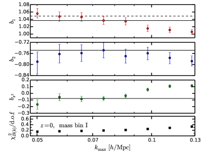
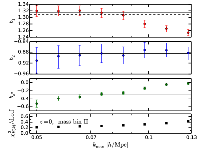
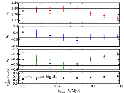
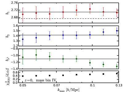
Figure 10: The best-fitting values of the bias parameters only from the bispectrum at $z=0$ as a function $k_{\rm max}$. Our fiducial choice at $k_{{\rm max},B(k)}=0.065h/$Mpc is highlighted with a black solid line. As a reference, the value of $b_{1}$ preferred by joint fitting with the power spectrum is indicated with a black dashed line.

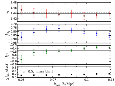
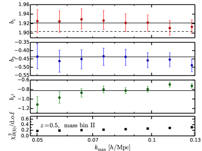
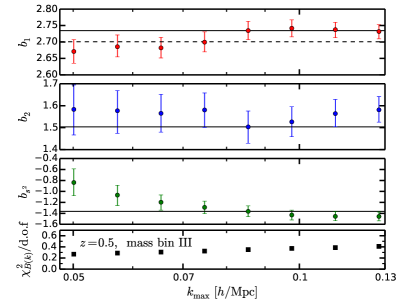
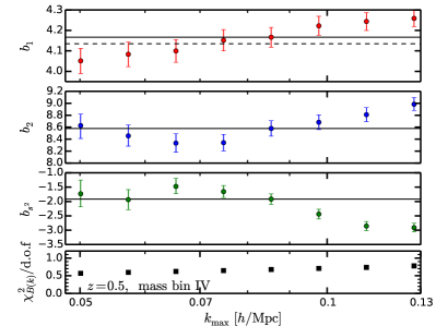
Figure 11: Same as Fig. 10, but at $z=0.5$.

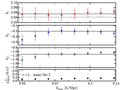
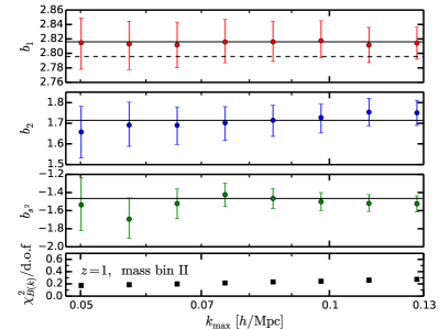
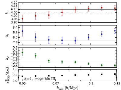
Figure 12: Same as Fig. 10, but at $z=1$.

As we discussed in §. II.3, the bispectrum is useful to access the second-order bias parameters, since the tree-level bispectrum depends only on the bias parameters up to second order. In other words, however, it is necessary to carefully investigate the valid range of the tree-level bispectrum. Here we show the fitting results using the bispectrum alone in our simulation. A set of free parameters is $(b_{1},b_{2},b_{s^{2}})$ in this case. Note that this analysis is slightly different from that in previous work Baldauf et al. (2012): we vary $b_{1}$ as a free parameter, while the authors in Baldauf et al. (2012) fixed the value of $b_{1}$ taken from the halo-matter power spectrum. Since we intend to combine the power spectrum with the bispectrum and we have already seen that there exists an anti-correlation between $b_{1}$ and $b_{\rm 3nl}$ in the joint fit, it is helpful to isolate the information only from the bispectrum.

Figs. 10-12 show bias parameters derived at $z=0$, 0.5 and 1, respectively, from our MCMC fitting as a function of $k_{\rm max}$. As found in Baldauf et al. (2012), we see non-zero second-order tidal bias $b_{s^{2}}$ for a variety of halo mass bins and redshifts. In addition the figures show that larger $k_{\rm max}$ results in general deviate more from low $k_{\rm max}$ ones with higher $\chi^{2}$ values, implying the PT model certainly breaks down at such small scales. Based upon these considerations we choose the valid range of the maximum wavenumber in the bispectrum in a redshift-dependent way: $k_{{\rm max},B(k)}=0.065(0.075)h$/Mpc at $z=0$ ($z=0.5$ or $1$). Note this choice is fully consistent with the $z=0$ result in Ref. Baldauf et al. (2012). Interestingly, this is achieved without adding information on the linear bias $b_{1}$ from the power spectrum. In fact the preferred values of $b_{1}$ only from the bispectrum tend to more deviate from ones in the joint-fit results at higher mass bins at higher redshift. This issue is also addressed in Figs. 6-8. When the preferred $b_{1}$ value from the bispectrum differs from that from the power spectrum, the bias values presented here could be different from those exhibited in the main text.

Appendix C Consistency check with the Galileon invariant approach

In §. II.4 we derived solutions up to third order for the simple co-evolution equations of dark matter and halo fluids starting from initial condition with purely local bias (i.e., local Lagrangian bias). As a matter of fact such solutions have been already derived in Ref. Chuen Chan et al. (2012) , but the authors took a different route which is based on Galileon symmetry in gravity. In this appendix we review the Galileon invariant approach and check that this approach is perfectly consistent with ours as expected.

In the Lagrangian picture, gravitational evolution of displacement field is solely governed by the velocity potential, $\Phi_{\rm v}$, defined by $\theta=\nabla^{2}\Phi_{\rm v}$. Since the halo distribution is a scalar under translations and rotation in three dimensional space, it should be written down in terms of scalar invariants of $\nabla_{i}\nabla_{j}\Phi_{\rm v}$. It is known that there are only three such invariants in three dimensional space, so called ‘Galileons’ Nicolis et al. (2009):

$$\mathcal{G}_{1} = \nabla^{2}\Phi_{\rm v},$$ (72)

$$\mathcal{G}_{2} = (\nabla_{i}\nabla_{j}\Phi_{\rm v})^{2}-(\nabla^{2}\Phi_{\rm v})^{2},$$ (73)

$$\mathcal{G}_{3} = (\nabla^{2}\Phi_{\rm v})^{3}+2(\nabla_{i}\nabla_{j}\Phi_{\rm v})(\nabla_{j}\nabla_{k}\Phi_{\rm v})(\nabla_{k}\nabla_{i}\Phi_{\rm v})-3(\nabla_{i}\nabla_{j}\Phi_{\rm v})^{2}\nabla^{2}\Phi_{\rm v}.$$ (74)

Ref. Chuen Chan et al. (2012) rewrote the co-evolution equations and derived the solutions in terms of Galileons. Since their approach solves the exactly same gravity system, it is quite natural to achieve the consistent solution with what we derived in §. II.4. Note that this approach does not hold if there exists a velocity bias, since relative motion between dark matter and halo fluids obviously breaks down the Galileon symmetry. Let us first begin with the second-order solution which is obtained as ($\epsilon=1$ and $y\to\infty$ in Eq. (95) in Ref. Chuen Chan et al. (2012))

$$\delta^{(2)}_{\rm h}=b_{1}^{\rm E}\delta^{(2)}+\frac{b^{\rm L}_{2}}{2}{\delta^{(1)}}^{2}-\frac{2}{7}b^{\rm L}_{1}\mathcal{G}_{2}^{(2)}(\Phi_{\rm v}),$$ (75)

where $\mathcal{G}_{2}^{(2)}(\Phi_{\rm v})$ in Fourier space is

$$\mathcal{G}_{2}^{(2)}(\Phi_{\rm v})(\mbox{\boldmath$q$}_{1},\mbox{\boldmath$q$}_{2})=\frac{\left(\mbox{\boldmath$q$}_{1}\cdot\mbox{\boldmath$q$}_{2}\right)^{2}}{q_{1}^{2}q_{2}^{2}}-1.$$ (76)

Thus the Fourier-transformed version of Eq. (75) matches Eq. (37). Note that the simple relation between Eulerian and Lagrangian bias, $b^{\rm E}_{2}=b^{\rm L}_{2}+(8/21)b^{\rm L}_{1}$ is used. Likewise the third-order solution is given by ($\epsilon=1$ and $y\to\infty$ in Eq. (99) in Ref. Chuen Chan et al. (2012))

$$\delta^{(3)}_{\rm h}=b_{1}^{\rm E}\delta^{(3)}+b^{\rm L}_{2}\delta^{(1)}\delta^{\rm L(2)}+\left(\frac{b^{\rm L}_{3}}{6}-\frac{b_{2}^{\rm L}}{2}\right){\delta^{(1)}}^{3}-\frac{2}{7}b^{\rm L}_{2}\delta^{(1)}\mathcal{G}_{2}^{(2)}(\Phi_{\rm v})-\frac{22}{126}b^{\rm L}_{1}\nabla[\mathcal{G}_{2}^{(2)}(\Phi_{\rm v}){\bf v}^{(1)}]-\frac{1}{9}b_{1}^{\rm L}\mathcal{G}_{2}^{(3)}(\Phi_{\rm v}),$$ (77)

where $\delta^{\rm L(2)}={\delta^{(1)}}^{2}+{\bf v}^{(1)}\cdot\nabla\delta^{(1)}+2\mathcal{G}^{(2)}_{2}/7$, and the (unsymmetrized) third-order part of the second-order Galileon is written in Fourier space as

$$\mathcal{G}_{2}^{(3)}(\Phi_{\rm v})(\mbox{\boldmath$q$}_{1},\mbox{\boldmath$q$}_{2},\mbox{\boldmath$q$}_{3}) = 2\left[\frac{\{\mbox{\boldmath$q$}_{1}\cdot(\mbox{\boldmath$q$}_{2}+\mbox{\boldmath$q$}_{3})\}^{2}}{q_{1}^{2}}\left\{\frac{1}{2}\frac{\mbox{\boldmath$q$}_{2}\cdot\mbox{\boldmath$q$}_{3}}{q_{2}^{2}q_{3}^{2}}-\frac{3}{7}\frac{1}{(\mbox{\boldmath$q$}_{2}+\mbox{\boldmath$q$}_{3})^{2}}\left[\frac{(\mbox{\boldmath$q$}_{2}\cdot\mbox{\boldmath$q$}_{3})^{2}}{q_{2}^{2}q_{3}^{2}}-1\right]\right\}\right.$$ (78)

$$\,\,\,-(\mbox{\boldmath$q$}_{2}+\mbox{\boldmath$q$}_{3})^{2}\left\{\frac{1}{2}\frac{\mbox{\boldmath$q$}_{2}\cdot\mbox{\boldmath$q$}_{3}}{q_{2}^{2}q_{3}^{2}}-\frac{3}{7}\frac{1}{(\mbox{\boldmath$q$}_{2}+\mbox{\boldmath$q$}_{3})^{2}}\left[\frac{(\mbox{\boldmath$q$}_{2}\cdot\mbox{\boldmath$q$}_{3})^{2}}{q_{2}^{2}q_{3}^{2}}-1\right]\right\}\left.\right]\delta_{0}(\mbox{\boldmath$q$}_{1})\delta_{0}(\mbox{\boldmath$q$}_{2})\delta_{0}(\mbox{\boldmath$q$}_{3}).$$

A tedious and long calculation shows that this solution exactly matches Eq. (40). Here also $b^{\rm E}_{3}=-(708/567)b^{\rm L}_{1}-(13/7)b^{\rm L}_{2}+b^{\rm L}_{3}$ is helpful to find the match. As discussed in Ref. Chuen Chan et al. (2012) (see also Assassi et al. (2014)), it is not necessary to start with Eq. (59) and there are duplicated terms in third-order terms in Eq. (59). However, this fact does not alter our discussion since all the nonlocal third-order terms can be summarized into the $b_{\rm 3nl}$ term anyway as shown in §. II.4 or in Ref. McDonald and Roy (2009).

Appendix D Predicting local bias parameters from the peak-background split with the universal mass function

In this appendix, we summarize how to predict the local bias parameters, $b_{1}$ and $b_{2}$, on the basis of a simple peak-background split Bardeen et al. (1986) combined with the universal halo mass function. For this purpose we here adopt the Sheth-Tormen (ST) fitting formula for the universal mass function Sheth and Tormen (1999). The similar contents can be found in the literature (see e.g., Saito et al. (2009)) and, this appendix follows the notation in Refs.Baldauf et al. (2011, 2012); Slosar et al. (2008).

The universal halo mass function basically assume that it depends only the peak hight $\nu$ defined as

$$\nu(R,z)=\frac{\delta_{\rm c}^{2}}{\sigma(R,z)^{2}},$$ (79)

where we set the density threshold $\delta_{\rm c}$ to be 1.686 based on the spherical collapse, and the variance of the matter fluctuation field smoothed over the scale $R$ is given by

$$\sigma^{2}(R,z)=\int\frac{k^{2}dk}{2\pi^{2}}\,P(k,z)|W(kR)|^{2},$$ (80)

with $W(kR)$ being the top-hat window function, i.e., $W(x)=3(\sin x-x\cos x)/x^{3}$. Here the Lagrangian radius $R$ is simply connected to the halo mass as $R=\{3M/(4\pi\overline{\rho}_{\rm m0})\}^{1/3}$. Note that $R$ does not depend on redshift. In the peak-background split, the local Lagrangian bias parameters are written down as

$$b_{1}^{\rm L}(M,z) = -\frac{1}{\overline{n}}\frac{2\nu}{\delta_{\rm c}}\frac{\partial n}{\partial\nu},$$ (81)

$$b_{2}^{\rm L}(M,z) = \frac{4}{\overline{n}}\frac{\nu^{2}}{\delta^{2}_{\rm c}}\frac{\partial^{2}n}{\partial\nu^{2}}+\frac{2}{\overline{n}}\frac{\nu}{\delta^{2}_{\rm c}}\frac{\partial n}{\partial\nu}.$$ (82)

In the case of the ST mass function, the derivatives are analytically expressed by

$$\frac{1}{\overline{n}}\frac{\partial n}{\partial\nu} = -\frac{q\nu-1}{2\nu}-\frac{p}{\nu\{1+(q\nu)^{p}\}},$$ (83)

$$\frac{1}{\overline{n}}\frac{\partial^{2}n}{\partial\nu^{2}} = \frac{p^{2}+\nu pq}{\nu^{2}\{1+(q\nu)^{p}\}}+\frac{(q\nu)^{2}-2q\nu-1}{4\nu^{2}},$$ (84)

where we adopt $(p,q)=(0.15,0.75)$. Finally we obtain the Eulerian local bias parameters using Eqs. (36) and (38).

References

- Komatsu et al. (2009) E. Komatsu, J. Dunkley, M. R. Nolta, C. L. Bennett, B. Gold, G. Hinshaw, N. Jarosik, D. Larson, M. Limon, L. Page, D. N. Spergel, M. Halpern, R. S. Hill, A. Kogut, S. S. Meyer, G. S. Tucker, J. L. Weiland, E. Wollack, and E. L. Wright, ApJS 180, 330 (2009), arXiv:0803.0547 .
- Komatsu et al. (2011) E. Komatsu, K. M. Smith, J. Dunkley, C. L. Bennett, B. Gold, G. Hinshaw, N. Jarosik, D. Larson, M. R. Nolta, L. Page, D. N. Spergel, M. Halpern, R. S. Hill, A. Kogut, M. Limon, S. S. Meyer, N. Odegard, G. S. Tucker, J. L. Weiland, E. Wollack, and E. L. Wright, ApJS 192, 18 (2011), arXiv:1001.4538 [astro-ph.CO] .
- Hinshaw et al. (2013) G. Hinshaw, D. Larson, E. Komatsu, D. N. Spergel, C. L. Bennett, J. Dunkley, M. R. Nolta, M. Halpern, R. S. Hill, N. Odegard, L. Page, K. M. Smith, J. L. Weiland, B. Gold, N. Jarosik, A. Kogut, M. Limon, S. S. Meyer, G. S. Tucker, E. Wollack, and E. L. Wright, ApJS 208, 19 (2013), arXiv:1212.5226 [astro-ph.CO] .
- Planck Collaboration et al. (2013) Planck Collaboration, P. A. R. Ade, N. Aghanim, C. Armitage-Caplan, M. Arnaud, M. Ashdown, F. Atrio-Barandela, J. Aumont, C. Baccigalupi, A. J. Banday, and et al., ArXiv e-prints (2013), arXiv:1303.5076 [astro-ph.CO] .
- Weinberg et al. (2013) D. H. Weinberg, M. J. Mortonson, D. J. Eisenstein, C. Hirata, A. G. Riess, and E. Rozo, Physics Reports 530, 87 (2013), arXiv:1201.2434 [astro-ph.CO] .
- Bernardeau et al. (2002) F. Bernardeau, S. Colombi, E. Gaztañaga, and R. Scoccimarro, Phys. Rep. 367, 1 (2002), arXiv:astro-ph/0112551 .
- Schlegel et al. (2009) D. Schlegel, M. White, and D. Eisenstein, in astro2010: The Astronomy and Astrophysics Decadal Survey, ArXiv Astrophysics e-prints, Vol. 2010 (2009) p. 314, arXiv:0902.4680 [astro-ph.CO] .
- Eisenstein et al. (2011) D. J. Eisenstein, D. H. Weinberg, E. Agol, H. Aihara, C. Allende Prieto, S. F. Anderson, J. A. Arns, É. Aubourg, S. Bailey, E. Balbinot, and et al., AJ 142, 72 (2011), arXiv:1101.1529 [astro-ph.IM] .
- Drinkwater et al. (2010) M. J. Drinkwater, R. J. Jurek, C. Blake, D. Woods, K. A. Pimbblet, K. Glazebrook, R. Sharp, M. B. Pracy, S. Brough, M. Colless, W. J. Couch, S. M. Croom, T. M. Davis, D. Forbes, K. Forster, D. G. Gilbank, M. Gladders, B. Jelliffe, N. Jones, I.-H. Li, B. Madore, D. C. Martin, G. B. Poole, T. Small, E. Wisnioski, T. Wyder, and H. K. C. Yee, MNRAS 401, 1429 (2010), arXiv:0911.4246 [astro-ph.CO] .
- Anderson et al. (2013a) L. Anderson, E. Aubourg, S. Bailey, F. Beutler, A. S. Bolton, J. Brinkmann, J. R. Brownstein, C.-H. Chuang, A. J. Cuesta, K. S. Dawson, D. J. Eisenstein, K. Honscheid, E. A. Kazin, D. Kirkby, M. Manera, C. K. McBride, O. Mena, R. C. Nichol, M. D. Olmstead, N. Padmanabhan, N. Palanque-Delabrouille, W. J. Percival, F. Prada, A. J. Ross, N. P. Ross, A. G. Sanchez, L. Samushia, D. J. Schlegel, D. P. Schneider, H.-J. Seo, M. A. Strauss, D. Thomas, J. L. Tinker, R. Tojeiro, L. Verde, D. H. Weinberg, X. Xu, and C. Yeche, ArXiv e-prints (2013a), arXiv:1303.4666 [astro-ph.CO] .
- Reid et al. (2012) B. A. Reid, L. Samushia, M. White, W. J. Percival, M. Manera, N. Padmanabhan, A. J. Ross, A. G. Sánchez, S. Bailey, D. Bizyaev, A. S. Bolton, H. Brewington, J. Brinkmann, J. R. Brownstein, A. J. Cuesta, D. J. Eisenstein, J. E. Gunn, K. Honscheid, E. Malanushenko, V. Malanushenko, C. Maraston, C. K. McBride, D. Muna, R. C. Nichol, D. Oravetz, K. Pan, R. de Putter, N. A. Roe, N. P. Ross, D. J. Schlegel, D. P. Schneider, H.-J. Seo, A. Shelden, E. S. Sheldon, A. Simmons, R. A. Skibba, S. Snedden, M. E. C. Swanson, D. Thomas, J. Tinker, R. Tojeiro, L. Verde, D. A. Wake, B. A. Weaver, D. H. Weinberg, I. Zehavi, and G.-B. Zhao, MNRAS 426, 2719 (2012), arXiv:1203.6641 [astro-ph.CO] .
- Anderson et al. (2013b) L. Anderson, E. Aubourg, S. Bailey, F. Beutler, V. Bhardwaj, M. Blanton, A. S. Bolton, J. Brinkmann, J. R. Brownstein, A. Burden, C.-H. Chuang, A. J. Cuesta, K. S. Dawson, D. J. Eisenstein, S. Escoffier, J. E. Gunn, H. Guo, S. Ho, K. Honscheid, C. Howlett, D. Kirkby, R. H. Lupton, M. Manera, C. Maraston, C. K. McBride, O. Mena, F. Montesano, R. C. Nichol, S. E. Nuza, M. D. Olmstead, N. Padmanabhan, N. Palanque-Delabrouille, J. Parejko, W. J. Percival, P. Petitjean, F. Prada, A. M. Price-Whelan, B. Reid, N. A. Roe, A. J. Ross, N. P. Ross, C. G. Sabiu, S. Saito, L. Samushia, A. G. Sanchez, D. J. Schlegel, D. P. Schneider, C. G. Scoccola, H.-J. Seo, R. A. Skibba, M. A. Strauss, M. E. C. Swanson, D. Thomas, J. L. Tinker, R. Tojeiro, M. V. Magana, L. Verde, D. A. Wake, B. A. Weaver, D. H. Weinberg, M. White, X. Xu, C. Yeche, I. Zehavi, and G.-B. Zhao, (2013b), arXiv:1312.4877v1 [astro-ph.CO] .
- Samushia et al. (2013) L. Samushia, B. A. Reid, M. White, W. J. Percival, A. J. Cuesta, G.-B. Zhao, A. J. Ross, M. Manera, É. Aubourg, F. Beutler, J. Brinkmann, J. R. Brownstein, K. S. Dawson, D. J. Eisenstein, S. Ho, K. Honscheid, C. Maraston, F. Montesano, R. C. Nichol, N. A. Roe, N. P. Ross, A. G. Sánchez, D. J. Schlegel, D. P. Schneider, A. Streblyanska, D. Thomas, J. L. Tinker, D. A. Wake, B. A. Weaver, and I. Zehavi, (2013), arXiv:1312.4899v1 [astro-ph.CO] .
- Beutler et al. (2013) F. Beutler, S. Saito, H.-J. Seo, J. Brinkmann, K. S. Dawson, D. J. Eisenstein, A. Font-Ribera, S. Ho, C. K. McBride, F. Montesano, W. J. Percival, A. J. Ross, N. P. Ross, L. Samushia, D. J. Schlegel, A. G. Sánchez, J. L. Tinker, and B. A. Weaver, (2013), arXiv:1312.4611v1 [astro-ph.CO] .
- Beutler et al. (2014) F. Beutler, S. Saito, J. R. Brownstein, C.-H. Chuang, A. J. Cuesta, W. J. Percival, A. J. Ross, N. P. Ross, D. P. Schneider, L. Samushia, A. G. Sánchez, H.-J. Seo, J. L. Tinker, C. Wagner, and B. A. Weaver, (2014), arXiv:1403.4599v1 [astro-ph.CO] .
- Zhao et al. (2013) G.-B. Zhao, S. Saito, W. J. Percival, A. J. Ross, F. Montesano, M. Viel, D. P. Schneider, D. J. Ernst, M. Manera, J. Miralda-Escude, N. P. Ross, L. Samushia, A. G. Sanchez, M. E. C. Swanson, D. Thomas, R. Tojeiro, C. Yeche, and D. G. York, MNRAS 436, 2038 (2013), arXiv:1211.3741 [astro-ph.CO] .
- Reid et al. (2014) B. A. Reid, H.-J. Seo, A. Leauthaud, J. L. Tinker, and M. White, ArXiv e-prints (2014), arXiv:1404.3742 .
- Blake et al. (2011a) C. Blake, S. Brough, M. Colless, C. Contreras, W. Couch, S. Croom, T. Davis, M. J. Drinkwater, K. Forster, D. Gilbank, M. Gladders, K. Glazebrook, B. Jelliffe, R. J. Jurek, I.-H. Li, B. Madore, D. C. Martin, K. Pimbblet, G. B. Poole, M. Pracy, R. Sharp, E. Wisnioski, D. Woods, T. K. Wyder, and H. K. C. Yee, MNRAS 415, 2876 (2011a), arXiv:1104.2948 [astro-ph.CO] .
- Blake et al. (2011b) C. Blake, T. Davis, G. B. Poole, D. Parkinson, S. Brough, M. Colless, C. Contreras, W. Couch, S. Croom, M. J. Drinkwater, K. Forster, D. Gilbank, M. Gladders, K. Glazebrook, B. Jelliffe, R. J. Jurek, I.-H. Li, B. Madore, D. C. Martin, K. Pimbblet, M. Pracy, R. Sharp, E. Wisnioski, D. Woods, T. K. Wyder, and H. K. C. Yee, MNRAS 415, 2892 (2011b), arXiv:1105.2862 [astro-ph.CO] .
- Blake et al. (2011c) C. Blake, E. A. Kazin, F. Beutler, T. M. Davis, D. Parkinson, S. Brough, M. Colless, C. Contreras, W. Couch, S. Croom, D. Croton, M. J. Drinkwater, K. Forster, D. Gilbank, M. Gladders, K. Glazebrook, B. Jelliffe, R. J. Jurek, I.-H. Li, B. Madore, D. C. Martin, K. Pimbblet, G. B. Poole, M. Pracy, R. Sharp, E. Wisnioski, D. Woods, T. K. Wyder, and H. K. C. Yee, MNRAS 418, 1707 (2011c), arXiv:1108.2635 [astro-ph.CO] .
- Blake et al. (2011d) C. Blake, K. Glazebrook, T. M. Davis, S. Brough, M. Colless, C. Contreras, W. Couch, S. Croom, M. J. Drinkwater, K. Forster, D. Gilbank, M. Gladders, B. Jelliffe, R. J. Jurek, I.-H. Li, B. Madore, D. C. Martin, K. Pimbblet, G. B. Poole, M. Pracy, R. Sharp, E. Wisnioski, D. Woods, T. K. Wyder, and H. K. C. Yee, MNRAS 418, 1725 (2011d), arXiv:1108.2637 [astro-ph.CO] .
- Blake et al. (2012) C. Blake, S. Brough, M. Colless, C. Contreras, W. Couch, S. Croom, D. Croton, T. M. Davis, M. J. Drinkwater, K. Forster, D. Gilbank, M. Gladders, K. Glazebrook, B. Jelliffe, R. J. Jurek, I.-h. Li, B. Madore, D. C. Martin, K. Pimbblet, G. B. Poole, M. Pracy, R. Sharp, E. Wisnioski, D. Woods, T. K. Wyder, and H. K. C. Yee, MNRAS 425, 405 (2012), arXiv:1204.3674 [astro-ph.CO] .
- Contreras et al. (2013) C. Contreras, C. Blake, G. B. Poole, F. Marin, S. Brough, M. Colless, W. Couch, S. Croom, D. Croton, T. M. Davis, M. J. Drinkwater, K. Forster, D. Gilbank, M. Gladders, K. Glazebrook, B. Jelliffe, R. J. Jurek, I.-h. Li, B. Madore, D. C. Martin, K. Pimbblet, M. Pracy, R. Sharp, E. Wisnioski, D. Woods, T. K. Wyder, and H. K. C. Yee, MNRAS 430, 924 (2013), arXiv:1302.5178 [astro-ph.CO] .
- Scrimgeour et al. (2012) M. I. Scrimgeour, T. Davis, C. Blake, J. B. James, G. B. Poole, L. Staveley-Smith, S. Brough, M. Colless, C. Contreras, W. Couch, S. Croom, D. Croton, M. J. Drinkwater, K. Forster, D. Gilbank, M. Gladders, K. Glazebrook, B. Jelliffe, R. J. Jurek, I.-h. Li, B. Madore, D. C. Martin, K. Pimbblet, M. Pracy, R. Sharp, E. Wisnioski, D. Woods, T. K. Wyder, and H. K. C. Yee, MNRAS 425, 116 (2012), arXiv:1205.6812 [astro-ph.CO] .
- Takada et al. (2012) M. Takada, R. Ellis, M. Chiba, J. E. Greene, H. Aihara, N. Arimoto, K. Bundy, J. Cohen, O. Doré, G. Graves, J. E. Gunn, T. Heckman, C. Hirata, P. Ho, J.-P. Kneib, O. Le Fèvre, L. Lin, S. More, H. Murayama, T. Nagao, M. Ouchi, M. Seiffert, J. Silverman, L. Sodré, Jr, D. N. Spergel, M. A. Strauss, H. Sugai, Y. Suto, H. Takami, and R. Wyse, ArXiv e-prints (2012), arXiv:1206.0737 [astro-ph.CO] .
- Adams et al. (2011) J. J. Adams, G. A. Blanc, G. J. Hill, K. Gebhardt, N. Drory, L. Hao, R. Bender, J. Byun, R. Ciardullo, M. E. Cornell, S. L. Finkelstein, A. Fry, E. Gawiser, C. Gronwall, U. Hopp, D. Jeong, A. Kelz, R. Kelzenberg, E. Komatsu, P. J. MacQueen, J. Murphy, P. S. Odoms, M. Roth, D. P. Schneider, J. R. Tufts, and C. P. Wilkinson, ApJS 192, 5 (2011), arXiv:1011.0426 [astro-ph.CO] .
- Levi et al. (2013) M. Levi, C. Bebek, T. Beers, R. Blum, R. Cahn, D. Eisenstein, B. Flaugher, K. Honscheid, R. Kron, O. Lahav, P. McDonald, N. Roe, D. Schlegel, and representing the DESI collaboration, ArXiv e-prints (2013), arXiv:1308.0847 [astro-ph.CO] .
- Laureijs et al. (2011) R. Laureijs, J. Amiaux, S. Arduini, J. . Auguères, J. Brinchmann, R. Cole, M. Cropper, C. Dabin, L. Duvet, A. Ealet, and et al., ArXiv e-prints (2011), arXiv:1110.3193 [astro-ph.CO] .
- Cooray and Sheth (2002) A. Cooray and R. Sheth, Phys. Rep. 372, 1 (2002), arXiv:astro-ph/0206508 .
- Seljak (2000) U. Seljak, MNRAS 318, 203 (2000), astro-ph/0001493 .
- Behroozi et al. (2010) P. S. Behroozi, C. Conroy, and R. H. Wechsler, ApJ 717, 379 (2010), arXiv:1001.0015 [astro-ph.CO] .
- Reddick et al. (2012) R. M. Reddick, R. H. Wechsler, J. L. Tinker, and P. S. Behroozi, ArXiv e-prints (2012), arXiv:1207.2160 [astro-ph.CO] .
- Hearin and Watson (2013) A. P. Hearin and D. F. Watson, MNRAS 435, 1313 (2013), arXiv:1304.5557 [astro-ph.CO] .
- Zentner et al. (2013) A. R. Zentner, A. P. Hearin, and F. C. v. d. Bosch, (2013), arXiv:1311.1818v1 [astro-ph.CO] .
- Leauthaud et al. (2011) A. Leauthaud, J. Tinker, P. S. Behroozi, M. T. Busha, and R. H. Wechsler, ApJ 738, 45 (2011), arXiv:1103.2077 [astro-ph.CO] .
- Tinker et al. (2013) J. L. Tinker, A. Leauthaud, K. Bundy, M. R. George, P. Behroozi, R. Massey, J. Rhodes, and R. Wechsler, (2013), arXiv:1308.2974v1 [astro-ph.CO] .
- Guo et al. (2014) H. Guo, Z. Zheng, I. Zehavi, H. Xu, D. J. Eisenstein, D. H. Weinberg, N. A. Bahcall, A. A. Berlind, J. Comparat, C. K. McBride, A. J. Ross, D. P. Schneider, R. A. Skibba, M. E. C. Swanson, J. L. Tinker, R. Tojeiro, and D. A. Wake, ArXiv e-prints (2014), arXiv:1401.3009 [astro-ph.CO] .
- Cole et al. (2005) S. Cole, W. J. Percival, J. A. Peacock, P. Norberg, C. M. Baugh, C. S. Frenk, I. Baldry, J. Bland-Hawthorn, T. Bridges, R. Cannon, M. Colless, C. Collins, W. Couch, N. J. G. Cross, G. Dalton, V. R. Eke, R. De Propris, S. P. Driver, G. Efstathiou, R. S. Ellis, K. Glazebrook, C. Jackson, A. Jenkins, O. Lahav, I. Lewis, S. Lumsden, S. Maddox, D. Madgwick, B. A. Peterson, W. Sutherland, and K. Taylor, MNRAS 362, 505 (2005), astro-ph/0501174 .
- Tegmark et al. (2006) M. Tegmark, D. J. Eisenstein, M. A. Strauss, D. H. Weinberg, M. R. Blanton, J. A. Frieman, M. Fukugita, J. E. Gunn, A. J. S. Hamilton, G. R. Knapp, R. C. Nichol, J. P. Ostriker, N. Padmanabhan, W. J. Percival, D. J. Schlegel, D. P. Schneider, R. Scoccimarro, U. Seljak, H. Seo, M. Swanson, A. S. Szalay, M. S. Vogeley, J. Yoo, I. Zehavi, K. Abazajian, S. F. Anderson, J. Annis, N. A. Bahcall, B. Bassett, A. Berlind, J. Brinkmann, T. Budavari, F. Castander, A. Connolly, I. Csabai, M. Doi, D. P. Finkbeiner, B. Gillespie, K. Glazebrook, G. S. Hennessy, D. W. Hogg, Ž. Ivezić, B. Jain, D. Johnston, S. Kent, D. Q. Lamb, B. C. Lee, H. Lin, J. Loveday, R. H. Lupton, J. A. Munn, K. Pan, C. Park, J. Peoples, J. R. Pier, A. Pope, M. Richmond, C. Rockosi, R. Scranton, R. K. Sheth, A. Stebbins, C. Stoughton, I. Szapudi, D. L. Tucker, D. E. vanden Berk, B. Yanny, and D. G. York, Phys. Rev. D 74, 123507 (2006), arXiv:astro-ph/0608632 .
- Yamamoto et al. (2010) K. Yamamoto, G. Nakamura, G. Hütsi, T. Narikawa, and T. Sato, Phys. Rev. D 81, 103517 (2010), arXiv:1004.3231 [astro-ph.CO] .
- Oka et al. (2014) A. Oka, S. Saito, T. Nishimichi, A. Taruya, and K. Yamamoto, MNRAS (2014), 10.1093/mnras/stu111, arXiv:1310.2820 [astro-ph.CO] .
- Kaiser (1984) N. Kaiser, ApJ 284, L9 (1984).
- Fry and Gaztanaga (1993) J. N. Fry and E. Gaztanaga, ApJ 413, 447 (1993), astro-ph/9302009 .
- Sheth and Tormen (1999) R. K. Sheth and G. Tormen, MNRAS 308, 119 (1999), astro-ph/9901122 .
- Tinker et al. (2008) J. Tinker, A. V. Kravtsov, A. Klypin, K. Abazajian, M. Warren, G. Yepes, S. Gottlöber, and D. E. Holz, ApJ 688, 709 (2008), arXiv:0803.2706 .
- Pollack et al. (2012) J. E. Pollack, R. E. Smith, and C. Porciani, MNRAS 420, 3469 (2012), arXiv:1109.3458 [astro-ph.CO] .
- Pollack et al. (2013) J. E. Pollack, R. E. Smith, and C. Porciani, (2013), arXiv:1309.0504v1 [astro-ph.CO] .
- Jeong and Komatsu (2009) D. Jeong and E. Komatsu, ApJ 691, 569 (2009), arXiv:0805.2632 .
- Saito et al. (2011) S. Saito, M. Takada, and A. Taruya, Phys. Rev. D 83, 043529 (2011), arXiv:1006.4845 [astro-ph.CO] .
- Nishizawa et al. (2012) A. J. Nishizawa, M. Takada, and T. Nishimichi, ArXiv e-prints (2012), arXiv:1212.4025 [astro-ph.CO] .
- McDonald and Roy (2009) P. McDonald and A. Roy, J. Cosmology Astropart. Phys 8, 20 (2009), arXiv:0902.0991 [astro-ph.CO] .
- Matsubara (2011) T. Matsubara, Phys. Rev. D 83, 083518 (2011), arXiv:1102.4619 [astro-ph.CO] .
- Baldauf et al. (2012) T. Baldauf, U. Seljak, V. Desjacques, and P. McDonald, ArXiv e-prints (2012), arXiv:1201.4827 [astro-ph.CO] .
- Chuen Chan et al. (2012) K. Chuen Chan, R. Scoccimarro, and R. K. Sheth, ArXiv e-prints (2012), arXiv:1201.3614 [astro-ph.CO] .
- McDonald (2006) P. McDonald, Phys. Rev. D 74, 103512 (2006), arXiv:astro-ph/0609413 .
- Assassi et al. (2014) V. Assassi, D. Baumann, D. Green, and M. Zaldarriaga, ArXiv e-prints (2014), arXiv:1402.5916 [astro-ph.CO] .
- Kehagias et al. (2013) A. Kehagias, J. Noreña, H. Perrier, and A. Riotto, (2013), arXiv:1311.0786v1 [astro-ph.CO] .
- Seljak et al. (2009) U. Seljak, N. Hamaus, and V. Desjacques, Physical Review Letters 103, 091303 (2009), arXiv:0904.2963 [astro-ph.CO] .
- Percival and Schäfer (2008) W. J. Percival and B. M. Schäfer, MNRAS 385, L78 (2008), arXiv:0712.2729 .
- Desjacques and Sheth (2010) V. Desjacques and R. K. Sheth, Phys. Rev. D 81, 023526 (2010), arXiv:0909.4544 [astro-ph.CO] .
- Desjacques et al. (2010) V. Desjacques, M. Crocce, R. Scoccimarro, and R. K. Sheth, Phys. Rev. D 82, 103529 (2010), arXiv:1009.3449 [astro-ph.CO] .
- Seljak and McDonald (2011) U. Seljak and P. McDonald, J. Cosmology Astropart. Phys 11, 039 (2011), arXiv:1109.1888 [astro-ph.CO] .
- Okumura et al. (2012a) T. Okumura, U. Seljak, and V. Desjacques, J. Cosmology Astropart. Phys 11, 014 (2012a), arXiv:1206.4070 [astro-ph.CO] .
- Okumura et al. (2012b) T. Okumura, U. Seljak, P. McDonald, and V. Desjacques, J. Cosmology Astropart. Phys 2, 010 (2012b), arXiv:1109.1609 [astro-ph.CO] .
- Vlah et al. (2012) Z. Vlah, U. Seljak, P. McDonald, T. Okumura, and T. Baldauf, J. Cosmology Astropart. Phys 11, 009 (2012), arXiv:1207.0839 [astro-ph.CO] .
- Vlah et al. (2013) Z. Vlah, U. Seljak, T. Okumura, and V. Desjacques, J. Cosmology Astropart. Phys 10, 053 (2013), arXiv:1308.6294 [astro-ph.CO] .
- Blazek et al. (2013) J. Blazek, U. Seljak, Z. Vlah, and T. Okumura, ArXiv e-prints (2013), arXiv:1311.5563 [astro-ph.CO] .
- Matsubara (2008) T. Matsubara, Phys. Rev. D 77, 063530 (2008), arXiv:0711.2521 .
- Taruya et al. (2010) A. Taruya, T. Nishimichi, and S. Saito, Phys. Rev. D 82, 063522 (2010), arXiv:1006.0699 [astro-ph.CO] .
- Fry (1996) J. N. Fry, ApJ 461, L65 (1996).
- Taruya (2000) A. Taruya, ApJ 537, 37 (2000), arXiv:astro-ph/9909124 .
- Hui and Parfrey (2008) L. Hui and K. P. Parfrey, Phys. Rev. D 77, 043527 (2008), arXiv:0712.1162 .
- Catelan et al. (1998) P. Catelan, F. Lucchin, S. Matarrese, and C. Porciani, MNRAS 297, 692 (1998), astro-ph/9708067 .
- Springel (2005) V. Springel, MNRAS 364, 1105 (2005), arXiv:astro-ph/0505010 .
- Desjacques et al. (2009) V. Desjacques, U. Seljak, and I. T. Iliev, MNRAS 396, 85 (2009), arXiv:0811.2748 .
- Percival et al. (2013) W. J. Percival, A. J. Ross, A. G. Sanchez, L. Samushia, A. Burden, R. Crittenden, A. J. Cuesta, M. V. Magana, M. Manera, F. Beutler, C.-H. Chuang, D. J. Eisenstein, S. Ho, C. K. McBride, F. Montesano, N. Padmanabhan, B. Reid, S. Saito, D. P. Schneider, H.-J. Seo, R. Tojeiro, and B. A. Weaver, (2013), arXiv:1312.4841v1 [astro-ph.CO] .
- Lewis and Bridle (2002) A. Lewis and S. Bridle, Phys. Rev. D 66, 103511 (2002), arXiv:astro-ph/0205436 .
- Carlson et al. (2009) J. Carlson, M. White, and N. Padmanabhan, Phys. Rev. D 80, 043531 (2009), arXiv:0905.0479 [astro-ph.CO] .
- Nishimichi et al. (2009) T. Nishimichi, A. Shirata, A. Taruya, K. Yahata, S. Saito, Y. Suto, R. Takahashi, N. Yoshida, T. Matsubara, N. Sugiyama, I. Kayo, Y. Jing, and K. Yoshikawa, PASJ 61, 321 (2009), arXiv:0810.0813 .
- Baldauf et al. (2013) T. Baldauf, U. Seljak, R. E. Smith, N. Hamaus, and V. Desjacques, ArXiv e-prints (2013), arXiv:1305.2917 [astro-ph.CO] .
- Hamaus et al. (2013) N. Hamaus, B. D. Wandelt, P. M. Sutter, G. Lavaux, and M. S. Warren, ArXiv e-prints (2013), arXiv:1307.2571 [astro-ph.CO] .
- Sato and Matsubara (2013) M. Sato and T. Matsubara, ArXiv e-prints (2013), arXiv:1304.4228 [astro-ph.CO] .
- Sheth et al. (2013) R. K. Sheth, K. C. Chan, and R. Scoccimarro, Phys. Rev. D 87, 083002 (2013), arXiv:1207.7117 [astro-ph.CO] .
- Bardeen et al. (1986) J. M. Bardeen, J. R. Bond, N. Kaiser, and A. S. Szalay, ApJ 304, 15 (1986).
- Elia et al. (2012) A. Elia, A. D. Ludlow, and C. Porciani, MNRAS 421, 3472 (2012), arXiv:1111.4211 [astro-ph.CO] .
- Desjacques (2008) V. Desjacques, Phys. Rev. D 78, 103503 (2008), arXiv:0806.0007 .
- Schmidt et al. (2012) F. Schmidt, D. Jeong, and V. Desjacques, ArXiv e-prints (2012), arXiv:1212.0868 [astro-ph.CO] .
- Biagetti et al. (2014) M. Biagetti, V. Desjacques, A. Kehagias, and A. Riotto, ArXiv e-prints (2014), 1405.1435 [astro-ph.CO] .
- Musso et al. (2012) M. Musso, A. Paranjape, and R. K. Sheth, MNRAS 427, 3145 (2012), arXiv:1205.3401 [astro-ph.CO] .
- Paranjape et al. (2013a) A. Paranjape, R. K. Sheth, and V. Desjacques, MNRAS 431, 1503 (2013a), arXiv:1210.1483 [astro-ph.CO] .
- Paranjape et al. (2013b) A. Paranjape, E. Sefusatti, K. C. Chan, V. Desjacques, P. Monaco, and R. K. Sheth, MNRAS 436, 449 (2013b), arXiv:1305.5830 [astro-ph.CO] .
- Villaescusa-Navarro et al. (2014) F. Villaescusa-Navarro, F. Marulli, M. Viel, E. Branchini, E. Castorina, E. Sefusatti, and S. Saito, J. Cosmology Astropart. Phys 3, 011 (2014), arXiv:1311.0866 [astro-ph.CO] .
- Note (1) Ref. Taruya (2000) has already derived such solutions in an exactly same way with ours, but investigated nonlocal terms in terms of stochastic bias in the halo-halo power spectrum.
- Nicolis et al. (2009) A. Nicolis, R. Rattazzi, and E. Trincherini, Phys. Rev. D 79, 064036 (2009), arXiv:0811.2197 [hep-th] .
- Saito et al. (2009) S. Saito, M. Takada, and A. Taruya, Phys. Rev. D 80, 083528 (2009), arXiv:0907.2922 .
- Baldauf et al. (2011) T. Baldauf, U. Seljak, and L. Senatore, J. Cosmology Astropart. Phys 4, 6 (2011), arXiv:1011.1513 [astro-ph.CO] .
- Slosar et al. (2008) A. Slosar, C. Hirata, U. Seljak, S. Ho, and N. Padmanabhan, J. Cosmology Astropart. Phys 8, 031 (2008), arXiv:0805.3580 .