Spanning the full Poincaré sphere with polariton Rabi oscillations

Abstract

We propose theoretically and demonstrate experimentally a generation of light pulses whose polarization varies temporally to cover selected areas of the Poincaré sphere with tunable swirling speed and total duration ($1\text{\,}\mathrm{ps}$ and $10\text{\,}\mathrm{ps}$ respectively in our implementation). The effect relies on the Rabi oscillations of two polarized fields in the strong coupling regime, excited by two counter-polarized and delayed pulses. The interferences of the oscillating fields result in the precession of the Stokes vector of the emitted light while polariton lifetime imbalance results in its drift from a circle on the sphere of controllable radius to a single point at long times. The positioning of the initial and final states allows to engineer the type of polarization spanning, including a full sweeping of the Poincaré sphere. The universality and simplicity of the scheme should allow for the deployment of time varying polarization fields at a technologically exploitable level.

Introduction

A new dimension has been literally opened for the control and manipulation of light with “polarization shaping” brixner01a ; sato13a . This makes the most out of the vectorial nature of light by determining its time evolution not only in phase and amplitude but also in its state of polarization. Since the interaction of light and matter is polarization sensitive, the control of this additional degree of freedom has allowed to outbeat the performances of light in most of its usual applications, such as photon ionization brixner04a , sub-wavelength localization aeschlimann07a or timing with zeptosecond precision kohler11a . Proposals abound as to its future applications in both a classical and quantum context brif10a . Beyond the extension of the concept of pulse shaping to encompass polarization, there has been as well increasing demand for time-independent but spatially varying polarization beams brown10a such as cylindrical vector beams youngworth00a . When providing all the states of polarization to realize so-called “full Poincaré beams” beckley10a , these also demonstrate advantages in similar endeavors, such as boosted scattering or sub-wavelength localization beckley10a . They also allow direct industrial applications in laser micro-processing, such as improving the efficiency and quality of processes like drilling holes for fuel-injection nozzles nolte99a , processing of silicon wafers meier07a or the machining of medical stent devices breitling_book04a . A new chapter of optics with fundamental as well as applied benefits has therefore been started with the availability of beams with a nontrivial dynamics of polarization.

Here we show that semiconductor microcavities kavokin_book11a in the strong exciton-photon coupling regime weisbuch92a offer a convenient and powerful platform to bring together these two twists on polarized light, by providing full Poincaré beams in time. This is implemented in a largely self-contained integrated device of micrometer size which does not rely on extrinsic processing of the signal. As such, this considerably improves on the unwieldy complexity of the setups required to generate polarization shaping and full Poincaré beams independently, that both come with their respective limitations. Indeed, since conventional solid state lasers typically emit light with a fixed linear polarization baranov_book13a , and optical nano-antennas also generally radiate a fixed polarization determined by their geometrical structure rodriguez13a ; banafsheh13a , the synthesizing of a desired polarization in space lerman10a or time brixner01a is an involved process. Time varying polarization is particularly demanding as it requires a combination of liquid crystals, spatial light modulators, interferometers and computer ressources with construction algorithms as well as state of the art pulse-shaping techniques, that all together make up a complex setup and impose some restrictions, such as the duration of the pulse polachek06a . The dynamics in our experiment takes place in a femtosecond timescale, as in many pulse shaping counteparts, but unlike these cases, it has no intrinsic restriction to a particular timescale and turning to other systems with Rabi frequencies of different magnitudes, the same dynamics can be realized with today’s technology in timeranges that run from attoseconds (with plexitons schlather13a ; vasa13a ) to milliseconds (with nanomechanical oscillators faust13a ). Our scheme also offers a tunable and undemanding control of which area to span on the Poincaré sphere and can be realized with any polarized fields that supports strong coupling, not only light. These results should allow to disseminate the usage of time-dependent polarization beams in a wide variety of platforms, including its extension to the quantum regime by powering the mechanism with quantum Rabi oscillations.

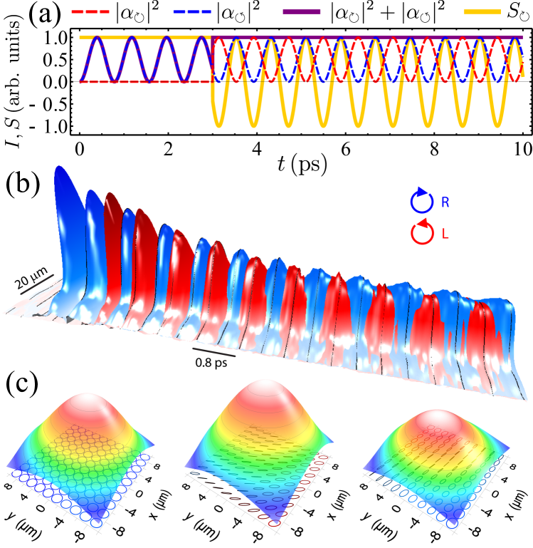
Figure 1: Rabi oscillations of polarized beams. (a) Rabi oscillations (theory) in i) one polarization only (till $t\approx$3\text{\,}\mathrm{ps}$$), resulting in an oscillating intensity (purple line) of constant polarization (yellow line), and ii) in two polarizations, reversing the pattern of oscillations. (b) Experimental observation of the effect through the cavity field (along the diameter of the Gaussian spot of $20\text{\,}\mathrm{\SIUnitSymbolMicro m}$ over a $10\text{\,}\mathrm{ps}$ duration) with left (red) and right (blue) circular polarization as a false color plot. In the experiment, the leakage of photons results in an exponential decay of the signal. See also Supplementary Movies S1 and S2. (c) Spatial distributions of the density and polarization at $200\text{\,}\mathrm{fs}$ time intervals during one of the initial cycles after the second pulse arrival. As can be seen while the emitted intensity remains basically constant (height scale in c) the resulting polarization is strongly affected by the Rabi oscillations (mutual oscillations in b and polarization map in c). The polarization can also be made homogeneous or not spatially.

Principle of the mechanism

The effect is based on the superposition of coherent states of different polarizations in the regime of Rabi oscillations norris94a . In some basis, say left ($\circlearrowleft$) and right ($\circlearrowright$) circular polarization, the state of the system is described by four complex amplitudes $\alpha_{p}$ and $\beta_{p}$ with $p=\circlearrowleft$, $\circlearrowright$ the state of polarization of the coherent photon $\alpha$ and exciton $\beta$ fields, with wavefunction $|{\psi(t)}\rangle=|{\alpha_{\circlearrowleft}(t),\beta_{\circlearrowleft}(t)}\rangle|{\alpha_{\circlearrowright}(t),\beta_{\circlearrowright}(t)}\rangle$, where we have written the coupled exciton-photon fields in the same ket vectors. Since there is no coupling between the polarizations in the linear regime of our experiment, each component evolves independently with the second quantized Hamiltonian $\sum_{p}g({a_{p}^{\dagger}}b_{p}+a_{p}{b_{p}^{\dagger}})$ for the ladder operators $a_{p}$ (for the photon) and $b_{p}$ (exciton), at resonance and in the rotating frame. Leaving aside for a moment the pulsed excitation to simply consider the initial state, the solution reads laussy09a :

$$\alpha_{p}(t)=\alpha_{p}(0)\cos(gt+\phi_{p})-i\beta_{p}(0)\sin(gt+\phi_{p})\,,$$ (1)

The exciton solution reads similarly but it is not explicitly needed since we are concerned in the time dynamics of the optical field only, obtained by tracing over the excitons $|{\psi_{\alpha}(t)}\rangle=|{\alpha_{\circlearrowleft}(t)}\rangle|{\alpha_{\circlearrowright}(t)}\rangle$ for $|{\alpha_{p}}\rangle=\exp(-|\alpha_{p}|^{2}/2)\sum_{k=0}^{\infty}\alpha_{p}^{k}|{k}\rangle/\sqrt{k!}$ the coherent state of cavity photons with complex amplitude $\alpha_{p}$ in the polarization $p$. In the following, we will call $\phi_{\alpha}=\phi_{\circlearrowright}-\phi_{\circlearrowleft}$ the relative optical phase between the two photon fields at $t=0$, and $\phi_{\beta}$ that between the exciton fields, which will play an important role and which, in the experiment will be controlled by the time delay between the exciting pulses. From Eq. (1), it is apparent that the exciton field is needed only as an initial condition. The state can be written in any of the familiar forms to represent polarization, such as Stokes or Jones vectors. In terms of the latter, the state of polarization reads:

$$\begin{pmatrix}\alpha_{\leftrightarrow}(t)\\ \alpha_{\updownarrow}(t)\end{pmatrix}=\frac{\alpha_{\circlearrowleft}(t)}{\sqrt{2}}\begin{pmatrix}1\\ i\end{pmatrix}+\frac{\alpha_{\circlearrowright}(t)}{\sqrt{2}}\begin{pmatrix}1\\ -i\end{pmatrix}\,,$$ (2)

with $\alpha_{\leftrightarrow,\updownarrow}$ the electromagnetic field components of the light in the linear polarization basis, emitted by the cavity in the rotating frame. One can then straightforwardly obtain the intensity $\langle{a_{p}^{\dagger}}a_{p}\rangle$ and degree of polarization $S_{p}=(\langle{a_{p}^{\dagger}}a_{p}\rangle-\langle{a_{q}^{\dagger}}a_{q}\rangle)/(\langle{a_{p}^{\dagger}}a_{p}\rangle+\langle{a_{q}^{\dagger}}a_{q}\rangle)$ in any basis through Jones calculus or, equivalently, the transformations $a_{\leftrightarrow}=(a_{\circlearrowleft}+a_{\circlearrowright})/\sqrt{2}$, $a_{\updownarrow}=i(a_{\circlearrowleft}-a_{\circlearrowright})/\sqrt{2}$ and $a_{\neswarrow/\nwsearrow}=((1\pm i)a_{\circlearrowleft}+(1\mp i)a_{\circlearrowright})/2$.

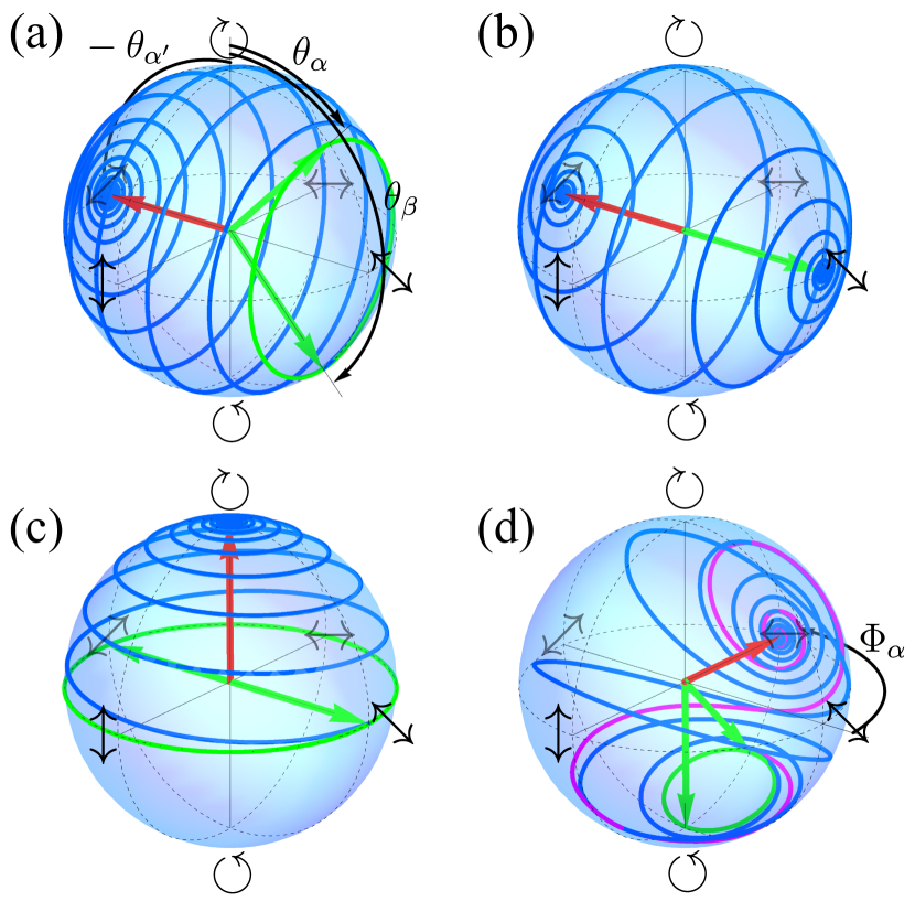
Figure 2: Dynamics of polarization on the Poincaré sphere (theory). The green arrows, defined by the angles $\theta_{\alpha}$ and $\theta_{\beta}$, fix the circle of polarization in absence of decay ($\gamma=0$) by intersecting the meridian of azimuthal angle $\phi_{\alpha}$. The red arrow, defined by the angle $\theta_{\alpha}^{\prime}$, fixes the point of long-time polarization. In presence of decay, $\gamma\neq 0$, the trajectory of the polarization, in blue, drifts from the green circle to the red final point. (a) Span of the Poincaré sphere excluding a spherical cap of antidiagonal polarization, by setting $R_{\alpha}=0.41$, $R_{\beta}=2.41$ and $R_{\alpha}^{\prime}=-1$. (b) Span of the full Poincaré sphere from the antidiagonal to the diagonal pole, by setting $R_{\alpha}=1-\epsilon$, $R_{\beta}=1+\epsilon$ and $R_{\alpha}^{\prime}=-1$ for $\epsilon\rightarrow 0$. (c) Span of the northern hemisphere of the Poincaré sphere in circular polarization, by setting $R_{\alpha}=1-\epsilon$, $R_{\beta}=-1$ and $R_{\alpha}^{\prime}\rightarrow\infty$ with $\epsilon\rightarrow 0$. (d) Distorted spanning of the sphere by choosing close initial and final points, by setting $R_{\alpha}=0$, $R_{\beta}=-2/3$, $R_{\alpha}^{\prime}=1$ and $\Phi_{\alpha}=\pi/2$. Parameters common to all cases: blue trajectories with $\gamma=1$ and the purple trajectory with $\gamma=3$.

Figure 1(a) shows a simple illustration of this polarized Rabi dynamics in the left-right circular polarization basis. The intermittent transfer of light to the exciton field through Rabi oscillations results in a temporary switch-off of the cavity emission in the corresponding polarization. By synchronizing them so that the cavity always emits in some polarization, one obtains a signal of constant intensity but of oscillating polarization defined by their superposition, which describes a circle on the Poincaré sphere during one period of oscillations (shown as a green trace in Fig. 2). The period, given by the polariton splitting, is roughly equal to $1\text{\,}\mathrm{ps}$ in our case. The circle is defined on the sphere, in a given basis (we will work in the circular one), by two couples of angles $(\theta_{\alpha,\beta},\Phi_{\alpha,\beta})$, defined by the ratios of polarization $R_{\alpha}=\alpha_{\circlearrowleft}/\alpha_{\circlearrowright}$ and $R_{\beta}=\beta_{\circlearrowleft}/\beta_{\circlearrowright}$ of the photon $\alpha$ and exciton $\beta$ fields at $t=0$, respectively. The relation follows straightforwardly by geometric construction as:

$$\theta_{\xi}=2\arccos(1/\sqrt{1+|R_{\xi}|^{2}})\,,$$ (3a)

$$\Phi_{\xi}=\phi_{\xi}+\arg R_{\xi}\,,$$ (3b)

for $\xi=\alpha$, $\beta$. This is illustrated in Fig. 2(a), where the case $\Phi_{\xi}=0$, $\theta_{\alpha}=\pi/4$ and $\theta_{\beta}=3\pi/4$ is shown. In the particular case where $\theta_{\alpha}=\theta_{\beta}$ and $\Phi_{\alpha}=\Phi_{\beta}$, the circle reduces to a point, i.e., to a constant polarization. This case corresponds to choices of $\alpha_{p}$ and $\beta_{p}$ that define a polariton, i.e., an eigenstate of the system with no temporal dynamics. The polarization of light is then fixed to that of the corresponding polariton.

Spanning the sphere thanks to polariton features

We can now take advantage of a feature that is usually regarded as a shortcoming of microcavity polaritons, but that in our case will turn the simple effect just proposed into a mechanism that powers a new type of light. There is a significant lifetime imbalance of the two types of polaritons dominici14a , with the upper polariton $|{\mathrm{U_{p}}}\rangle=|{\alpha_{p},\beta_{p}}\rangle$—where $\alpha_{p}=\beta_{p}$—being much more short-lived as compared to the lower polariton $|{\mathrm{L_{q}}}\rangle=|{\alpha_{q},\beta_{q}}\rangle$—where $\alpha_{q}=-\beta_{q}$—regardless of the polarizations $p,q$. The upper polariton lifetime is typically of the order of $2\text{\,}\mathrm{ps}$ while the lower polariton lifetime is of the order of $10\text{\,}\mathrm{ps}$. These values can however be tuned by orders of magnitude with the already existing technology steger13a . This results in time-dependent Rabi oscillations that converge toward a monotonously decaying signal as the population of the upper polaritons “evaporates” and only lower polaritons remain.

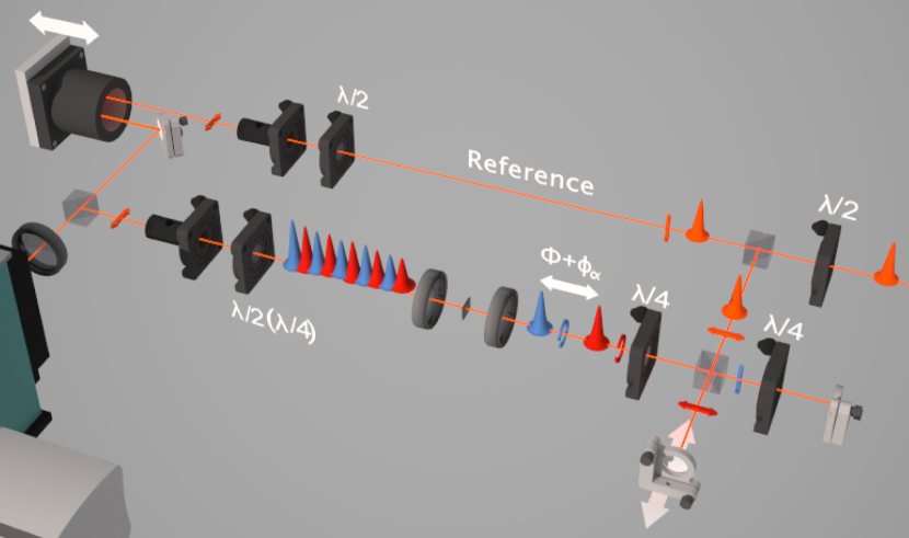
Figure 3: Setup that implements the effect experimentally. The effect is implemented and observed with a time-resolved digital holography setup for counter-polarized double pulse experiments. The fs pulses train is first split in a reference beam ($\updownarrow$) and a signal beam ($\leftrightarrow$). This latter is further divided into twin pulses of equal $\leftrightarrow$ linear polarizations, of which, only one, upon double passage onto a $\lambda/4$ plate, becomes $\updownarrow$ linear. After rejoining their paths, the twins are made counter-circular (by use of a second $\lambda/4$ plate). Their mutual delay can be set on a Rabi period scale ($\Phi$) and wavelength order ($\phi_{\alpha}$). Sample emission is then filtered in polarization and let to interfere with the reference on the camera, before digital elaboration.

The overall dynamics of polarization is therefore that which starts by describing the circle of the Rabi dynamics in absence of dissipation, with a continuous drift towards the fixed point of polarization of the lower polariton. The final state can be parametrized in the same way with a couple of angles $(\theta^{\prime}_{\alpha},\Phi^{\prime}_{\alpha})$, by making a rotation of the polariton basis. This introduces the parameters $\alpha_{p}^{\prime}=(\alpha_{p}-\beta_{p})/\sqrt{2}$ and $R_{\alpha}^{\prime}=\alpha^{\prime}_{\circlearrowright}/\alpha^{\prime}_{\circlearrowleft}$ from which one obtains the angles $\theta^{\prime}_{\alpha}=2\arccos(1/\sqrt{1+|R^{\prime}_{\alpha}|^{2})}$ and $\Phi^{\prime}_{\alpha}=\phi_{\alpha}+\arg R^{\prime}_{\alpha}$ (cf. Eqs. (3)).

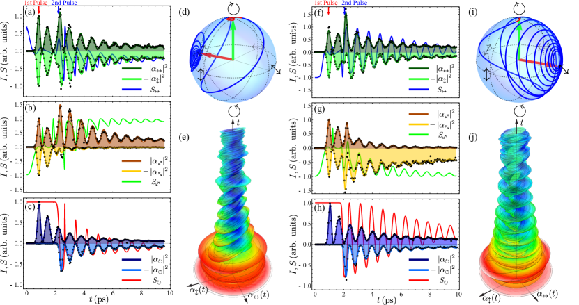
Figure 4: Experimental Observation of the effect Rabi in-phase experiment (a-e), i.e., the Rabi oscillations from the two different pulses start with the same phase, and Rabi antiphase experiment (f-j), i.e., the Rabi oscillations start with an opposite phase. The experimental data (a-c, f-h, black dots) is fitted by the theoretical model (solid lines), providing the amplitudes $|\alpha_{p,q}|^{2}$ and degrees of polarizations $S_{p}$. The dynamics of polarization can be displayed on the Poincaré sphere (d,i), demonstrating the rapid transition to the linear polarization in (d) and the spanning of the full hemisphere polarization in (i). (e,j) $2\textrm{D}+t$ representation of the field polarization, the radius and the color (from red to blue) of the ellipses are scaled on the instantaneous total intensity and polarization fields, respectively.

By fixing with the effective polariton state of Eq. (1), on a meridian defined by $\phi_{\alpha}$, the initial and final states through the three couples of angles $(\theta_{\alpha},\Phi_{\alpha})$, $(\theta_{\beta},\Phi_{\beta})$ (for the initial circle normal to the meridian) and $(\theta^{\prime}_{\alpha},\Phi^{\prime}_{\alpha})$ (for the final point on the meridian), one can thus span the Poincaré sphere of polarization in essentially any desired way. The exact trajectory is obtained by including decay in the dynamics of the coupled fields. This is achieved by turning to a dissipative master equation delvalle_book10a $\dot{\rho}=i\left[\rho,H\right]+\mathcal{L}\rho$ for the four-fields density matrix, with $\mathcal{L}\rho$ the Lindblad super-operator. Assuming radiative decays of all fields (with their corresponding decay rates $\gamma_{a,b}$) as well as a mechanism dephasing the upper polariton, that can be either radiative decay $\gamma_{\mathrm{U}}^{\mathrm{R}}$ or pure dephasing $\gamma_{\mathrm{U}}^{\phi}$, and incoherent pumping $P_{b}$ from the exciton reservoir, we are brought to a Liouvillian in the form dominici14a $\mathcal{L}\rho=\sum_{p=\circlearrowright,\circlearrowleft}\Big{[}\frac{\gamma_{a}}{2}\mathcal{L}_{a_{p}}+\frac{\gamma_{b}}{2}\mathcal{L}_{b_{p}}+\frac{P_{b}}{2}\mathcal{L}_{{b_{p}^{\dagger}}}+\frac{\gamma_{\mathrm{U}}^{\mathrm{R}}}{2}\mathcal{L}_{u_{p}}+\frac{\gamma_{\mathrm{U}}^{\phi}}{2}\mathcal{L}_{{u_{p}^{\dagger}}u_{p}}\Big{]}\rho$, with $\mathcal{L}_{c}\rho=2c\rho{c^{\dagger}}-{c^{\dagger}}c\rho-\rho{c^{\dagger}}c$ for the generic operator $c$. This too can be solved in closed-form. For the observables of interest, the solution remains fully defined by complex amplitudes:

$$\alpha_{p}(t)=\Bigg{[}\alpha_{p}(0)\cosh(Rt/4+i\phi_{p})\\ -\left(\frac{\beta_{p}(0)G+\alpha_{p}(0)\Gamma}{R}\right)\sinh(Rt/4+i\phi_{p})\Bigg{]}\exp(-\gamma t/4)\,,$$ (4)

where we have introduced:

$$\gamma=\gamma_{a}+\gamma_{b}+\gamma_{\mathrm{U}}-P_{b}\,, \Gamma=P_{b}-\gamma_{b}+\gamma_{a}\,,$$ (5a)

$$G=i4g+\gamma_{\mathrm{U}}\,, R=\sqrt{G^{2}+\Gamma^{2}}\,,$$ (5b)

$$\gamma_{\mathrm{U}}=\gamma_{\mathrm{U}}^{\mathrm{R}}+\gamma_{\mathrm{U}}^{\phi}\,.$$ (5c)

Equation (5c) states that it does not matter which mechanism is responsible for the loss of the upper polaritons, only the total decay rate enters the dynamics.

Some illustrative examples of this dynamics are shown in Fig. 2. In all cases, green arrows point at the initial states and the red one at the fixed point of the asymptotic final state. The green circle shows the polarization cycle in absence of dissipation and the blue trajectory the spanning of the Poincaré sphere for the system parameters (given in the caption). Panel (a) shows the spanning excluding a spherical cap of antidiagonal polarization. Panel (b) includes it by reducing the circle to a single point, thereby achieving a full spanning of the sphere. Panel (c) shows the spanning of a hemisphere only and from the horizontal/diagonal basis equator towards the right-circular polarization, again, covering a different area merely by tuning the parameters $\alpha_{p}$, $\beta_{q}$ and $\phi_{\alpha}$. Panel (d) shows two interesting variations of this effect: first, by choosing close points on the sphere, one can obtain a twisted trajectory, covering different areas with different speeds and, therefore, opening the possibility for emitters of pseudo-random polarization given the uncertainty at which time the photon will be emitted along an intricate path on the sphere. Second, by varying the Rabi period, which can be achieved by tuning the coupling strength, or the decay rates, one can vary the number of loops around the sphere.

Experimental implementation

To implement these effects in the laboratory, we used a GaAs polariton microcavity in the regime of Rabi oscillations described in previous works dominici14a ; ballarini13a . A sketch of our setup is shown in Fig. 3, which is based on the principles of the time-resolved digital holography dominici14a . Two femtosecond pulses with adjustable delay and polarization excite the system. The pulses are initially linearly polarized and subsequently passed through quarter wavelength plates to make them counter-circularly polarized. The energy spread of the pulses overlaps with both polariton branches and thus triggers Rabi oscillations between excitons and photons. After the 1st pulse, the lower and upper polaritons have the same circular polarization. After the 2nd pulse, the dynamics of polarization is triggered according to the principle of Eq. (4). By weighting adequately the two branches and by adjusting the optical phase between the two pulses, we are able to realize various cases of interest predicted by the theory. Some typical experimental observations are shown in Fig. 4, where we present the detected polarization in all the bases, namely (a) $\leftrightarrow$/$\updownarrow$, (b) $\nwsearrow$/$\neswarrow$ and (c) $\circlearrowleft$/$\circlearrowright$. We show in each case the intensity of light emitted in each component, $|\alpha_{p}|^{2}$ and the corresponding degree of polarization $S_{p}$. The points are experimental data and the lines are theory fits with the model presented above but supplemented with the dynamics of excitation by femtosecond polarized pulses. While all polarizations are measured experimentally, only two polarizations are needed by the theory to obtain the other ones. We have checked the consistency of the model and the observation by fitting polarizations in all bases and by their reconstruction from one basis only. Experimentally, only the photonic field is accessible, but the theory allows to reach the exciton field as well. Therefore, we are able to reconstruct the polarization dynamics, as shown in Fig. 4 (d,i), and (e,j) with a 3D (2D+time) representation of the polarization. The effective quantum state can also be reconstructed dominici14a . The dynamics is more clearly visualized on the Poincaré sphere. Figure 4 shows how the beam of light emitted by the microcavity provides an ultra-fast sweeping of, in these cases, a hemisphere of the Poincaré sphere, and with two speeds of relaxation similarly to the cases of the theoretical model shown in Fig. 2(d). In all cases, the agreement between theory and experiment is excellent.

Extensions and applications

In the literature, a variety of multiple polarized beams are implemented by setting space profiles with different polarization. A noticeable example is that of radial (hedgehog) or azimuthal polarization field states realizable, e.g., by use of Q-plate devices cardano12a . Here, we have used essentially spatially homogeneous profiles in the experiments, as seen in the time-space chart in Fig. 1(b,c), to focus on the time dynamics instead. Nevertheless, a spatially dependent polarization could also be combined with the temporal dynamics we have highlighted. One of the easiest space patternings would consist of sending the second pulse with a slight angle of incidence (i.e., a $\Delta k_{\alpha}$) with respect to the first one. In this case, while co-polarized beams would give interference fringes of amplitude, Rabi-oscillating in time (hence moving with a $g/\Delta k_{\alpha}$ velocity), in the case of counter-polarized beams, all the dynamics discussed in the present work could be obtained with an associated phase delay between the fringes. Each fringe could be made time-oscillating in polarization and with a phase offset with respect to each other, giving rise to a flow of polarization waves with Rabi time period and settable space period, the whole drifting towards the fixed polarization state of the LP polariton. Such effects are beyond the scope of this work but give a hint as to the rich patterns of polarization texture that are within reach, when powered by the dynamics of polariton fluids carusotto13a .

Supplementary Material

Supplementary Movie S1. The ultrafast imaging sequence of the opposing polarization densities in the experiment of Fig. 1(b,c). The map is over a $30\text{\times}30\text{\,}\mathrm{\SIUnitSymbolMicro m}$ area and along a $10\text{\,}\mathrm{ps}$ duration with time step of $50\text{\,}\mathrm{fs}$.

Supplementary Movie S2. The dynamics in a time-space representation, with the amplitude of the two circular polarizations plotted vs a central diameter and time.

References

- (1) Brixner, T. & Gerber, G. Femtosecond polarization pulse shaping. Opt. Lett. 26, 557 (2001).
- (2) Sato, M. et al. Terahertz polarization pulse shaping with arbitrary field control. Nat. Photon. 7, 724 (2013).
- (3) Brixner, T. et al. Quantum control by ultrafast polarization shaping. Phys. Rev. Lett. 92, 208301 (2004).
- (4) Aeschlimann, M. et al. Adaptive subwavelength control of nano-optical fields. Nature 446, 301 (2007).
- (5) Köhler, J., Wollenhaupt, M., Bayer, T., Sarpe, C. & Baumert, T. Zeptosecond precision pulse shaping. Opt. Express 19, 11638 (2011).
- (6) Brif, C., Chakrabarti, R. & Rabitz, H. Control of quantum phenomena: past, present and future. New J. Phys. 12, 075008 (2010).
- (7) Brown, T. G. & Zhan, Q. Focus issue: Unconventional polarization states of light. Opt. Express 18, 10775 (2010).
- (8) Youngworth, K. S. & Brown, T. G. Focusing of high numerical aperture cylindrical-vector beams. Opt. Express 7, 77 (2000).
- (9) Beckley, A. M., Brow, T. G. & Alonso, M. A. Full poincaré beams. Opt. Express 10, 10777 (2010).
- (10) Nolte, S. et al. Polarization effects in ultrashort-pulse laser drilling. Appl. Phys. A 68, 563 (1999).
- (11) Meier, M., Romano, V. & Feurer, T. Material processing with pulsed radially and azimuthally polarized laser radiation. Appl. Phys. A 86, 329 (2007).
- (12) Breitling, D., Föhl, C., Dausinger, F., Kononenko, T. & Konov, V. Femtosecond Technology for Technical and Medical Applications. (Springer, London, 2004).
- (13) Kavokin, A., Baumberg, J. J., Malpuech, G. & Laussy, F. P. Microcavities (Oxford University Press, 2011), 2 edn.
- (14) Weisbuch, C., Nishioka, M., Ishikawa, A. & Arakawa, Y. Observation of the coupled exciton-photon mode splitting in a semiconductor quantum microcavity. Phys. Rev. Lett. 69, 3314 (1992).
- (15) Baranov, A. & Tournie, E. Semiconductor Lasers, Fundamentals and Applications (Elsevier, 2013).
- (16) Rodríguez-Fortuño, F. J. et al. Near-field interference for the unidirectional excitation of electromagnetic guided modes. Science 19, 328 (2013).
- (17) Abasahl, B., Dutta-Gupta, S., Santschi, C. & Martin, O. J. F. Coupling strength can control the polarization twist of a plasmonic antenna. Nano Lett. 13, 4575 (2013).
- (18) Lerman, G. M., Stern, L. & Levy, U. Generation and tight focusing of hybridly polarized vector beams. Opt. Express 26, 27650 (2010).
- (19) Polachek, L., Oron, D. & Silberberg, Y. Full control of the spectral polarization of ultrashort pulses. Opt. Lett. 31, 631 (2006).
- (20) Steger, M. et al. Long-range ballistic motion and coherent flow of long-lifetime polaritons. Phys. Rev. B 88, 235314 (2013).
- (21) Schlather, A. E., Large, N., Urban, A. S., Nordlander, P. & Halas, N. J. Near-field mediated plexcitonic coupling and giant Rabi splitting in individual metallic dimers. Nano Lett. 13, 3281 (2013).
- (22) Vasa, P. et al. Real-time observation of ultrafast Rabi oscillations between excitons and plasmons in metal nanostructures with J-aggregates. Nat. Photon. 7, 128 (2013).
- (23) Faust, T., Rieger, J., Seitner, M. J., Kotthaus, J. P. & Weig, E. M. Coherent control of a classical nanomechanical two-level system. Nat. Phys. 9, 485 (2013).
- (24) Norris, T. et al. Time-resolved vacuum Rabi oscillations in a semiconductor quantum microcavity. Phys. Rev. B 50, 14663 (1994).
- (25) Laussy, F. P., del Valle, E. & Tejedor, C. Luminescence spectra of quantum dots in microcavities. I. Bosons. Phys. Rev. B 79, 235325 (2009).
- (26) Dominici, L. et al. Ultrafast control and rabi oscillations of polaritons. Phys. Rev. Lett. 113, 226401 (2014).
- (27) del Valle, E. Microcavity Quantum Electrodynamics (VDM Verlag, 2010).
- (28) Ballarini, D. et al. All-optical polariton transistor. Nat. Comm. 4, 1778 (2013).
- (29) Cardano, F. et al. Polarization pattern of vector vortex beams generated by q-plates with different topological charges. App. Optics 51, C1 (2012).
- (30) Carusotto, I. & Ciuti, C. Quantum fluids of light. Rev. Mod. Phys. 85, 299 (2013).