Entanglement Spectrum of a Random Partition:
Connection with the Localization Transition

Abstract

We study the entanglement spectrum of a translationally-invariant lattice system under a random partition, implemented by choosing each site to be in one subsystem with probability $p\in[0,1]$. We apply this random partitioning to a translationally-invariant (i.e., clean) topological state, and argue on general grounds that the corresponding entanglement spectrum captures the universal behavior about its disorder-driven transition to a trivial localized phase. Specifically, as a function of the partitioning probability $p$, the entanglement Hamiltonian $H_{A}$ must go through a topological phase transition driven by the percolation of a random network of edge-states. As an example, we analytically derive the entanglement Hamiltonian for a one-dimensional topological superconductor under a random partition, and demonstrate that its phase diagram includes transitions between Griffiths phases.

In recent years, systematic studies of quantum entanglement have greatly advanced our understanding of topological states of matter that cannot be adiabatically connected to a trivial product state. For example, topological entanglement entropy is directly related to the total quantum dimension of fractional quasi-particles levinwen ; Kitaev_Preskill . More recently, there has been a growing interest in utilizing the full entanglement spectrum to extract other universal properties Li_Haldane , especially in chiral topological phases (e.g., quantum Hall states) or symmetry-protected topological phases (e.g., topological insulators). As a common feature, these phases have topologically-protected gapless excitations on a physical boundary. When the ground state is spatially cut into left and right halves, the low-lying part of the entanglement spectrum shares the same universal characteristics as the energy spectrum of these boundary excitations Li_Haldane ; Edge_1 ; Edge_2 ; Edge_3 ; Edge_4 ; Edge_5 ; Edge_7 .

A recent work studied the entanglement spectrum obtained from an extensive partition that divides a system into two extensive subsystems Hsieh_Fu . For topological states that support gapless edge states, the corresponding entanglement spectrum was found to encode a wealth of information about the universal quantum critical behavior that would arise at its phase transition to a trivial direct-product state, despite the fact that the system under study itself is non-critical. It has been further shown that the entanglement spectra of extensive partitions can be directly computed from the matrix product state or tensor network representation of ground-state wavefunctions Hsieh_Fu_Qi , which may offer insights into topological phase transitions Zhang ; santos ; hatsugai ; Borchmann .

In this Letter, we study the entanglement spectum generated from a random partition that spatially bipartitions a system in a probabilistic manner: each physical site is chosen to be in subsystem $B$ (or $A$) with a probability $p\in[0,1]$ (or $1-p$). We apply this random partition to a translationally-invariant (i.e., clean) topological state, and argue on general grounds that the corresponding entanglement spectrum reproduces the universal behavior about its disorder-driven transition to a trivial localized phase. As an example, we analytically derive the form of the entanglement Hamiltonian for a clean one-dimensional topological superconductor under random partition, and establish the entanglement phase diagram as a function of probability $p$, finding agreement with the physical phase diagram of a disordered superconductor Huse_Motrunich_Damle .

We begin by considering a translationally-invariant topological state, which can be either a topological insulator/superconductor or a bosonic symmetry-protected topological phase. It has been shown Hsieh_Fu that upon varying the geometry of $A$ and $B$ subsystems in an extensive partition, the corresponding entanglement Hamiltonian undergoes a gap-closing transition that lies in the same universality class as the transition to a topologically trivial state realized by tuning the physical Hamiltonian. This intriguing connection is not a coincidence, but follows from the nature of topological phase transitions, which are driven by the percolation of gapless edge-states. For example, the transition from a quantum Hall insulator to a trivial insulator is described by the quantum percolation of chiral edge-states in a Chalker-Coddington network model Chalker_Coddington . Extensive partitioning of a quantum Hall insulator precisely creates, in the low-lying part of the entanglement spectrum, a network of chiral edge states moving along the percolating borders between $A$ and $B$. This mapping explains why topological phase transitions and entanglement spectra of extensive partitions are intimately related. It further motivates us to study the random partitioning of a topological ground-state, for which the entanglement spectrum is expected to mimic the network model with randomness and thus connect with the localization transition.

We define the probabilistic partitioning of a clean, topological state $\ket{\Psi}$ as follows. We independently choose each physical site in the full system to be in the $B$ subsystem with probability $p$; the remaining sites are defined to be in subsystem $A$. A partial trace of the density matrix over sites in subsystem $B$ yields a reduced density matrix for the $A$ subsystem $\rho_{A}\equiv{\rm Tr}_{B}|\Psi\rangle\langle\Psi|$, which can be interpreted as the thermal density matrix at temperature $T=1$ for an entanglement Hamiltonian $H_{A}$: $\rho_{A}\equiv e^{-H_{A}}$.

Our goal is to determine the phase diagram of $H_{A}$ as a function of the partitioning probability $p$. First, when $p\rightarrow 0$, the probabilistic partitioning yields a vanishingly small $B$ subsystem, with most sites belonging to the $A$ subsystem. In this limit, the ground-state of the entanglement Hamiltonian, denoted by $\ket{\psi_{A}}$, must share the same topological index as the original ground state $\ket{\Psi}$. As $p\rightarrow 1$, however, most sites become part of the $B$ subsystem, so that $\ket{\psi_{A}}$ becomes a trivial product state over the disjoint regions of the $A$ subsystem, and hence must be topologically trivial. Since the topological character of $\ket{\psi_{A}}$ changes as we tune the partitioning probability $p$, we conclude that the entanglement Hamiltonian ${H}_{A}$ must go through a phase transition at some critical partitioning probability $p=p_{c}$. Physically, the transition is driven by the percolation of a random network of gapless edge-states propagating around traced-out regions of the $B$ subsystem, as in the case of the aforementioned checkerboard-type extensive partition. Even though the original state $\ket{\Psi}$ is translationally-invariant, the probabilistic partitioning procedure introduces randomness into the entanglement Hamiltonian $H_{A}$, with the probability $p$ effectively tuning disorder strength.

The phase diagram of the entanglement Hamiltonian as a function of $p$ satisfies additional constraints. For a given bipartition, the eigenvalue spectra of the reduced density matrices $\rho_{A}$ and $\rho_{B}$ are identical, though their Hilbert spaces are distinct. By definition, for a fixed partitioning probability $p$, the $B$ subsystem is, on average, equivalent to the $A$ subsystem obtained with a partitioning probability $1-p$. Therefore, the ensemble-averaged spectra of the entanglement Hamiltonians ${H}_{A}(p)$ and ${H}_{A}(1-p)$ must be identical. As a result, the presence of a phase transition in the entanglement Hamiltonian with partition probability $p$ implies another transition at probability $1-p$. In the case where the topological index of $\ket{\Psi}$ cannot be evenly divided between two subsystems, as is the case for topological insulators with a $\mathbb{Z}_{2}$ index or quantum Hall insulators with an odd Chern number, we further expect that $H_{A}$ exhibits at least a topological phase transition at partitioning probability $p=1/2$, when the two subsystems are equivalent on average.

For the remainder of the paper, we apply our random partitioning procedure to Kitaev’s model Kitaev for a clean one-dimensional $p$-wave superconductor, extract the phase diagram of the entanglement Hamiltonian as a function of partitioning probability, and demonstrate its correspondence with a disordered superconductor. The Kitaev model is described by the Hamiltonian

$$H= -w\sum_{n}\left(c^{\dagger}_{n+1}c_{n}+\text{h.c.}\right)+\sum_{n}\left(\Delta c^{\dagger}_{n+1}c^{\dagger}_{n}+\text{h.c.}\right)$$

$$-\mu\sum_{n}\left(c^{\dagger}_{n}c_{n}-\frac{1}{2}\right)$$ (1)

with fermion operators $c_{n}$, $c^{\dagger}_{n}$ satisfying canonical anti-commutation relations. To simplify the calculation below, we restrict ourselves to the case where $w=\Delta\in\mathbb{R}$. Introducing two species of Majorana fermions at each lattice site $\gamma_{n}\equiv c_{n}+c^{\dagger}_{n}$ and $\chi_{n}\equiv(c^{\dagger}_{n}-c_{n})/i$, we may write the Hamiltonian as

$${H}=\frac{iw}{2}\sum_{n}\left[\eta\gamma_{n}\chi_{n}+\chi_{n}\gamma_{n+1}\right]$$ (2)

where the dimensionless parameter $\eta\equiv\mu/2w$ distinguishes the topologically trivial strong pairing phase ($|\eta|>1$) and topologically non-trivial weak pairing phase ($|\eta|<1$). As shown in Figure 1, in the topological superconductor (TSC) phase, Majorana fermions couple more strongly across two adjacent lattice sites than within a lattice site, leading to two unpaired Majorana fermions at the ends of the chain. In the extreme limit when $\eta=0$ in the topological phase, pairs of Majorana fermions within lattice sites completely decouple. We will refer to this special point $\eta=0$ as the Kitaev limit of the Hamiltonian (2), which proves to be a useful starting point for our analysis below.

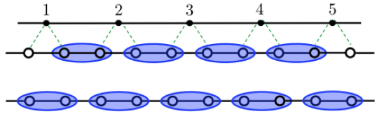
Figure 1: The two ground-states of the Kitaev $p$-wave superconductor with dimerization of Majorana fermions across (top) and within (bottom) lattice sites, corresponding to a TSC and a trivial $p$-wave superconductor, respectively.

Let $\ket{\Psi(\eta)}$ be the ground-state of the Kitaev Hamiltonian with parameter $|\eta|<1$ in the topological regime. Applying the random partitioning procedure to this ground-state, we trace over physical lattice sites (each of which contains two Majorana fermions) with probability $p$, and obtain an entanglement Hamiltonian $H_{A}(\eta;p)$. Clearly, $H_{A}(\eta;p)$ contains random couplings between sites in the $A$ subsystem, and mimics the physical Hamiltonian of a disordered superconductor, with the partitioning probability $p$ playing the role of disorder strength.

To derive $H_{A}(\eta;p)$, we note that the entanglement Hamiltonian of an $N$-site free fermion system such as the Kitaev model can only contain fermion bilinear terms Peschel . The spectrum of the entanglement Hamiltonian can be determined from the correlation matrices in the original ground-state $C_{nm}\equiv\braket{\Psi\,}{\,c^{\dagger}_{n}c_{n}\,}{\,\Psi}$ and $F_{nm}\equiv\braket{\Psi\,}{\,c^{\dagger}_{n}c^{\dagger}_{m}\,}{\,\Psi}$, by solving the eigenvalue problem Peschel :

$$(2\hat{C}-2\hat{F}-1)(2\hat{C}+2\hat{F}-1)\phi_{\ell}=\tanh^{2}\left(\frac{\epsilon_{\ell}}{2}\right)\phi_{\ell}$$ (3)

where $\epsilon_{\ell}$ is an eigenvalue of the entanglement Hamiltonian, with eigenvector $\phi_{\ell}$. Rewriting the complex fermions in terms of Majorana operators, we may define the $2N\times 2N$ skew-symmetric correlation matrix $\hat{\Gamma}$ for the Majorana fermions which has eigenvalues $\pm\tanh(\epsilon_{\ell}/2)$ Peschel_2 ; Supp_Material . Since we are interested in the low-lying part of the entanglement spectrum $\epsilon_{\ell}\rightarrow 0$, $\tanh(\epsilon_{\ell}/2)\rightarrow\epsilon_{\ell}/2$ and hence $\hat{\Gamma}$ satisfies:

$$2\hat{\Gamma}\phi_{\ell}\approx\pm\epsilon_{\ell}\phi_{\ell}$$ (4)

Therefore, the correlation matrix for Majorana fermions in the original ground-state is equivalent to the entanglement Hamiltonian acting on low-lying states $\epsilon_{\ell}\rightarrow 0$ in the entanglement spectrum. By building the correlation matrix for Majorana fermions in the ground-state $\ket{\Psi(\eta)}$, we may now construct the entanglement Hamiltonian for the Kitaev model after a random partition.

For arbitrary $\eta$, performing a random partition will generally produce an entanglement Hamiltonian with highly non-local couplings, due to the non-vanishing correlations between distant Majorana fermions in the ground state. However, for a sufficiently small $|\eta|$, i.e., when the system is close to the Kitaev limit, we may derive the form of $H_{A}(\eta;p)$ analytically. Let us first consider the case $\eta=0$, when pairs of Majorana fermions decouple. A single cut between two adjacent lattice sites then produces, in the entanglement spectrum of the $A$ subsystem, an unpaired Majorana fermion at the end of $A$. Aside from this, the entanglement spectrum at $\eta=0$ is identical to the energy spectrum (properly normalized) of decoupled Majorana pairs in the Kitaev Hamiltonian. Therefore, performing a random partition with several cuts will yield an $A$ subsystem that consists of disjoint segments, each of which hosts unpaired Majorana fermions at the two ends.

We now explicitly construct the entanglement Hamiltonian $H_{A}(\eta;p)$ near the Kitaev limit by perturbing away from $\eta=0$. As one may expect, a small $\eta$ induces a small coupling between the unpaired Majorana fermions at ends of disjoint segments with the rest of the $A$ subsystem. By an analytical calculation Supp_Material , we find that couplings between two Majorana fermions in $H_{A}(\eta;p)$ decrease exponentially with their separation in the original lattice. Therefore, it suffices to include nearest-neighbor couplings within subsystem $A$ only in $H_{A}(\eta;p)$.

Two types of nearest-neighbor couplings appear in $H_{A}(\eta;p)$. First, to leading order in $\eta$, couplings belonging to a connected sequence of sites in the $A$ subsystem are identical to those appearing in the original Kitaev Hamiltonian, after a proper normalization. Second, couplings between Majorana fermions belonging to different segments in the $A$ subsystem are computed from their two-point correlation function. If a series of $N$ consecutive lattice sites $-$ between sites $m-1$ and $m+N$ $-$ are determined to be within the $B$ subsystem and traced over in the random partition, a coupling will be induced between the Majorana fermions at the right and left edges of the two lattice sites, which is found to be proportional to $C(N)\equiv\langle\Psi(\eta)\,|\,i\chi_{m-1}\gamma_{m+N}\,|\,\Psi(\eta)\rangle$. An explicit calculation Supp_Material yields the result that at long distances, i.e. large $N$,

$$C(N)\sim\eta^{N}/\sqrt{N}+O(\eta^{N+1})$$ (5)

We then conclude that the entanglement Hamiltonian takes the form:

$${H}_{A}(\eta;p)=\frac{iw}{2}\sum_{n\in A}\eta\gamma_{n}\chi_{n}+\frac{iw}{2}\sum_{m>n\in A}f_{nm}\chi_{n}\gamma_{m}$$ (6)

where $f_{nm}$ has non-zero elements $f_{n,n+1}=1$ and $f_{nm}=C(m-n-1)$ if $n$ and $m$ label lattice sites at the right and left edges of two adjacent segments in the $A$ subsystem. The couplings in the entanglement Hamiltonian are illustrated in Fig. 2.

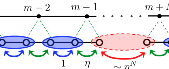
Figure 2: The entanglement Hamiltonian $H_{A}(\eta;p)$, derived in the Kitaev limit $|\eta|<<1$, consists of several couplings between adjacent Majorana fermions in the subsystem $A$. Blue and green hoppings between nearest-neighbor Majorana fermions appear with dimensionless coupling $1$ and $\eta$, respectively. Tracing over $N$ lattice sites induces a coupling $O(\eta^{N})$ between the dangling Majorana modes on the adjacent chains in the $A$ subsystem.

We now demonstrate that the topological character of the entanglement Hamiltonian (6) changes at a critical partitioning probability $p=1/2$. Specifically, we demonstrate that when $p<1/2$ the entanglement Hamiltonian in the $A$ subsystem supports an exponentially localized edge-state $\ket{\psi}$ at zero energy and corresponds to a topological superconductor phase, but that such a state does not exist for $p>1/2$.

To see this, we first note that a random partitioning of a chain with probability $p$ will produce an $A$ subsystem that consists of clusters of lattice sites. Let us now introduce a boundary in the $A$ subsystem and explicitly construct a zero-energy state of the entanglement spectrum under a random partition. Recall that an exact zero-energy left-boundary eigenstate of the translationally-invariant Kitaev Hamiltonian (2) takes the form $\ket{\psi}=(1,0,\eta,0,\eta^{2},0,\ldots)$, with $|\eta|<1$, in the basis of Majorana sites on a semi-infinite chain Kitaev . We find a similar zero-energy state can be obtained for the entanglement Hamiltonian (6) of the $A$ subsystem, which consists of consecutive clusters of sites of lengths $\{\ell_{k}\}$, each separated by distance $\{d_{k}\}$. An edge-state of the entanglement Hamiltonian now takes the form:

$$\ket{\psi_{A}}\propto \Bigg{(}\underbrace{1,0,\eta,0,\ldots,\eta^{\ell_{1}},0,}_{\text{1st cluster of sites}}\,{\frac{\eta^{\ell_{1}}}{C(d_{1})},0,\ldots,\frac{\eta^{\ell_{1}+\ell_{2}}}{C(d_{1})},0,\ldots}$$

$$\underbrace{\prod_{k=1}^{N-1}\frac{\eta^{\ell_{k}}}{C(d_{k})},0,\ldots,\eta^{\ell_{N}}\prod_{k=1}^{N-1}\frac{\eta^{\ell_{k}}}{C(d_{k})},0}_{N^{\mathrm{th}}\text{ cluster of sites}},\ldots\Bigg{)}$$ (7)

in a basis of Majorana sites in $A$. From the form of the two-point function computed previously we see that amplitude for the edge-state on the first Majorana site in the $N$th cluster of the $A$ subsystem is given by:

$$\psi_{N}=\prod_{k=1}^{N-1}\frac{\eta^{\ell_{k}}}{C(d_{k})}\sim\prod_{k=1}^{N-1}\eta^{\ell_{k}-d_{k}}=\eta^{\,\sum_{k}\ell_{k}-\sum_{k}d_{k}}$$ (8)

Now, if we consider the amplitude at the end of the chain, we see that $\psi_{N}\rightarrow\eta^{L_{A}-L_{B}}$ where $L_{A}$ and $L_{B}$ are the sizes of the $A$ and $B$ subsystems, respectively. For a system of size $L$, regardless of the probability distributions for the lengths $\{\ell_{k}\}$ and $\{d_{k}\}$, the sizes of the two subsystems are determined from the partitioning probability to be $L_{A}=(1-p)L$ and $L_{B}=pL$ in the thermodynamic limit $L\rightarrow+\infty$ so that

$$\psi_{N}\rightarrow\left[\eta^{1-2p}\right]^{L}$$ (9)

When $p<1/2$ we observe that the state (Entanglement Spectrum of a Random Partition: Connection with the Localization Transition) is an exact zero-energy eigenstate of the entanglement Hamiltonian. When $p>1/2$, however, the amplitude at the end of the chain diverges and the above state becomes non-normalizable for an infinite set of clusters.

The above calculation of an edge-state immediately implies that the entanglement Hamiltonian $H_{A}$ changes from being topologically non-trivial at partitioning probability $p<1/2$ to trivial when $p>1/2$, and hence must be critical at the point $p=1/2$. This transition can also be understood by integrating out the Majorana fermions in the interior of the clusters in the $A$ subsystem and constructing an effective entanglement Hamiltonian $H_{A}^{\mathrm{eff}}$ acting exclusively on the dangling Majorana modes at the ends of each cluster. In this case, $H_{A}^{\mathrm{eff}}$ will describe a dimerized Majorana fermion chain, in which two adjacent Majorana fermions correspond to sites separated by lengths $\{...\ell_{k},d_{k},\ell_{k+1},d_{k+1}...\}$ in the original lattice. The nearest-neighbor hopping in $A$, which is proportional to the corresponding correlation function in the ground-state, is determined by the lengths $\{d_{k}\}$ for intra-cluster hoppings or $\{\ell_{k+1}\}$ for inter-cluster hoppings. At $p=1/2$, the $A$ and $B$ subsystems are equivalent on average, so that the length distributions $\{\ell_{k}\}$ and $\{d_{k}\}$ are identical, and the ensemble of $H_{A}^{\mathrm{eff}}$ is translationally-invariant, instead of dimerized. The corresponding ground state of a one-dimensional Majorana fermion chain is well-known to be critical Fulga .

We now demonstrate that in the vicinity of $p=1/2$, the entanglement Hamiltonian is in Griffiths phases, characterized by a singularity in the density of states at zero energy due to the proliferation of segments of the topologically-ordered or trivial phase, respectively. Recall that when $p<1/2$, near $p=1/2$, the characteristic size of clusters in the $A$ subsystem is larger than that of the $B$ subsystem. Then, the dangling Majorana modes on adjacent clusters in the $A$ subsystem, separated by distance $x$ will mix to form localized bound-states with finite energy $\epsilon\sim\exp[c\,x\ln|\eta|]$, with $c>0$ a constant. Since the probability of such a configuration of sites in the $A$ subsystem is $p^{x}(1-p)^{2}$, the contribution of these low-energy modes to the density of states in the entanglement ground-state is Huse_Motrunich_Damle :

$$\rho(\epsilon)=\int_{0}^{\infty}dx\,(1-p)^{2}p^{x}\,\delta(\epsilon-e^{c\,x\ln|\eta|})\propto\frac{1}{\epsilon^{1-\beta(p)}}$$ (10)

with the non-universal exponent $\beta(p)\equiv\ln(p)/c\,\ln|\eta|$. The power-law singularity in the density of states signals the presence of a Griffiths region for an entanglement ground-state with $p$ near $1/2$, due to the proliferation of low-energy configurations of Majorana edge-modes dimerizing across lattice sites. $p>1/2$ also correspond to a Griffiths phase, with exponent $\beta(1-p)$ due to Majorana modes at the ends of the same chain forming bound-states with exponentially small energy. The two Griffiths phases at $p<1/2$ and $p>1/2$ are both characterized by a power-law singularity in the density of states at zero energy, but are topologically distinct, as shown by the presence and absence of zero-energy Majorana fermion at the boundary.

To summarize, we have introduced a random partitioning scheme to study the disorder-driven quantum critical behavior of a topological phase; applying this procedure to the one-dimensional $p$-wave superconductor yields an interesting phase diagram, consisting of two topologically distinct Griffiths phases separated by a critical point. The random-partitioning scheme may be naturally used to study spin-chains Fisher ; Yang , as well as higher-dimensional systems to numerically extract critical exponents of disorder-driven phase transitions, such as localization transitions in all symmetry classes of non-interacting topological phases Classification_1 ; Classification_2 . It might also be interesting to study the entanglement spectrum of fractional topological phases under a random partition, although the connection with topological phase transitions appears to be less direct.

I Supplementary Material

In this section, we briefly review the calculation of the entanglement Hamiltonian for the ground-state of a free-fermion system as presented in Peschel_SM ; Peschel_2_SM and compute the two-point correlation function between Majorana fermions on even and odd Majorana sites in the ground-state of the Kitaev chain Kitaev_SM , in the limit that the coupling $\eta\equiv\mu/2w$ is small. In the main text, this calculation is used to construct the associated entanglement Hamiltonian, which is directly proportional to the correlation matrix for the Majorana fermions in the ground-state, when acting on the low-lying states in the entanglement spectrum.

Appendix A The Entanglement Hamiltonian from a Bipartition of a Free-Fermion Ground State

For a free-fermion Hamiltonian, the entanglement Hamiltonian obtained after a bipartition of the ground-state $\ket{\Psi}$ may be determined entirely from the two-point correlation functions in the ground-state. For a free-fermion system, any $n$-point correlation function can be written as a sum over two-point functions by Wick s Theorem. Furthermore, the reduced density matrix $\rho_{A}$ is defined to reproduce all observables in the $A$ subsystem. Therefore, for a fermion number-conserving, free-fermion Hamiltonian, the reduced density matrix must take the form:

$$\rho_{A}=\frac{e^{-\mathcal{H}_{A}}}{Z}\hskip 21.68121pt\mathcal{H}_{A}\equiv\sum_{i,\,j\in A}h_{ij}c^{\dagger}_{i}c_{j}$$ (11)

with $Z\equiv\mathrm{Tr}\left[e^{-\mathcal{H}_{A}}\right]$ and fermion operators $c_{i}$, $c_{j}^{\dagger}$ satisfying canonical anti-commutation relations. In this case, we may explicitly diagonalize the entanglement Hamiltonian $\mathcal{H}_{A}$, and express the correlation matrix $C_{nm}\equiv\braket{c^{\dagger}_{n}c_{m}}$ (with $n,m\in A)$ evaluated in the ground-state in terms of the eigenvalues $\{\epsilon_{j}\}$ and eigenvectors $\{\phi_{j}\}$ of $\mathcal{H}_{A}$ as Peschel_SM :

$$C_{nm}=\mathrm{Tr}\left[\rho_{A}c^{\dagger}_{n}c_{m}\right]=\sum_{j}\phi^{*}_{j}(n)\phi_{j}(m)\left(e^{\epsilon_{j}}+1\right)^{-1}$$ (12)

In matrix form, this is equivalent to the statement that the entanglement Hamiltonian may be written as $(\mathcal{H}_{E})^{T}=\ln[(1-\hat{C})/\hat{C}]$, and that $\hat{C}$ solves the eigenvalue problem Peschel_2_SM :

$$(1-2\hat{C})\phi_{j}=\tanh\left(\frac{\epsilon_{j}}{2}\right)\phi_{j}$$ (13)

A similar calculation may be performed for a free-fermion Hamiltonian defined on $N$ lattice sites that only conserves fermion number parity. In this case, the expansion of an $n$-point function in terms of two-point correlators will include contributions from both the regular $C_{nm}\equiv\braket{c^{\dagger}_{n}c_{m}}$ and ‘anomalous’ correlation functions $F_{nm}\equiv\braket{c^{\dagger}_{n}c^{\dagger}_{m}}$. In order for the reduced density matrix to reproduce all observables in $A$, the entanglement Hamiltonian must also be a free-fermion Hamiltonian with pairing terms Peschel_SM , i.e. of the form:

$$\mathcal{H}_{E}=\sum_{n,m}\left[f_{nm}c^{\dagger}_{n}c_{m}+\Delta_{nm}c^{\dagger}_{n}c^{\dagger}_{m}+\mathrm{h.c.}\right]$$ (14)

As explained in Peschel_2_SM , we may diagonalize the Hamiltonian by Bogoliubov transformation, so that the $\hat{C}$ and $\hat{F}$ matrices now satisfy the eigenvalue problem:

$$(2\hat{C}-2\hat{F}-1)(2\hat{C}+2\hat{F}-1)\phi_{j}=\tanh^{2}\left(\frac{\epsilon_{j}}{2}\right)\phi_{j}$$ (15)

Equivalently, the entanglement Hamiltonian may be expressed in terms of Majorana operators $\gamma_{2n-1}\equiv c_{n}+c^{\dagger}_{n}$ and $\gamma_{2n}\equiv-i(c_{n}-c_{n}^{\dagger})$. In this case, $\mathcal{H}_{E}$ will only contain terms bilinear in the Majorana operators, and may be written in the form:

$$\mathcal{H}_{E}=\frac{i}{4}\sum_{n,m\in A}B_{nm}\gamma_{n}\gamma_{m}$$ (16)

with $\hat{B}$ a $2N\times 2N$ real, skew-symmetric matrix. We may diagonalize the entanglement Hamiltonian by block-diagonalizing $\hat{B}$ by an appropriate orthogonal transformation and bringing it into canonical form:

$$\mathcal{O}^{T}\hat{B}\mathcal{O}=\left(\begin{array}[]{cccccc}0&\epsilon_{1}&&&&\\ -\epsilon_{1}&0&&&&\\ &&0&\epsilon_{2}&&\\ &&-\epsilon_{2}&0&&\\ &&&&&\ddots\end{array}\right)$$ (22)

with $\mathcal{O}\in O(2N)$ so that the entanglement eigenvalues are $\pm\epsilon_{\ell}$. Taking the appropriate real linear combination of the Majorana operators $\{\gamma_{n}\}$ given by the eigenvectors of $\hat{B}$ that diagonalize the entanglement Hamiltonian, it is possible to compute the two-point correlation function $\Gamma_{nm}\equiv\braket{\gamma_{n}\gamma_{m}}$ $(n\neq m)$ in the original ground-state. Similar to the correlation function for a free-fermion system conserving fermion number, this yields the result Peschel_2_SM that $\Gamma$ solves the eigenvalue problem:

$$\hat{\Gamma}\phi_{\ell}=\pm\tanh\left(\frac{\epsilon_{\ell}}{2}\right)\phi_{\ell}$$ (23)

Therefore, in the limit $\epsilon_{\ell}\rightarrow 0$, we see that $2\hat{\Gamma}\phi_{\ell}\approx\pm\epsilon_{\ell}\phi_{\ell}$, so that the two-point function for Majorana fermions in the original ground-state is equivalent to the entanglement Hamiltonian when acting on the low-lying ($\epsilon_{\ell}\rightarrow 0$) states in the entanglement spectrum.

Appendix B The Two-Point Correlation Function for the Kitaev Majorana Chain

We now compute the two-point function for Majorana fermions in the ground-state of the Kitaev Hamiltonian Kitaev_SM

$$H= -w\sum_{n}\left(c^{\dagger}_{n+1}c_{n}+\text{h.c.}\right)+\sum_{n}\left(\Delta c^{\dagger}_{n+1}c^{\dagger}_{n}+\text{h.c.}\right)$$

$$-\mu\sum_{n}\left(c^{\dagger}_{n}c_{n}-\frac{1}{2}\right)$$ (24)

with $w=\Delta\in\mathbb{R}$. The complex fermion operators satisfy canonical anti-commutation relations $\{c_{n},c_{m}\}=\{c_{n}^{\dagger},c_{m}^{\dagger}\}=0$ and $\{c_{n},c^{\dagger}_{m}\}=\delta_{nm}$. In the topologically non-trivial phase, the ground-state of the Hamiltonian on an $N$-site chain with periodic boundary conditions takes the form of a BCS wavefunction with odd fermion parity:

$$\ket{\Psi}=\prod_{k\neq 0}\left[u_{k}+v_{k}\cdot a^{\dagger}_{k}a^{\dagger}_{-k}\right]a^{\dagger}_{0}\ket{0}$$ (25)

where the parameter $u_{k}$ is given by:

$$u_{k}^{2}=\frac{1}{2}\left(1+\frac{2w\cos k+\mu}{E(k)}\right)$$ (26)

with $u_{k}^{2}+v_{k}^{2}=1$. Here, the quantity $E(k)=\sqrt{(2w\cos k+\mu)^{2}+4w^{2}\sin^{2}k}$ is the bulk dispersion Kitaev_SM . We note that the non-vanishing correlation functions for the ground-state take the form:

$$\langle\Psi\,|\,c_{p}^{\dagger}c_{k}^{\dagger}\,|\,\Psi\rangle=\delta_{k,-p}\cdot u_{k}v_{k}$$ (27)

$$\langle\Psi\,|\,c^{\dagger}_{k}c_{p}\,|\,\Psi\rangle=\delta_{k,p}\cdot v_{k}^{2}$$ (28)

We now explicitly compute the two-point correlation functions for the Majorana fermions in the ground-state of the clean Kitaev chain. The real-space correlation functions for the complex fermions may be written by performing a Fourier transform:

$$\langle c^{\dagger}_{n}c^{\dagger}_{m}\rangle=\frac{1}{N}\sum_{k}e^{ik(m-n)}u_{k}v_{k}$$ (29)

$$\langle c^{\dagger}_{n}c_{m}\rangle=\frac{1}{N}\sum_{k}e^{ik(m-n)}v_{k}^{2}$$ (30)

Now, we define the Majorana operators $\gamma_{2n}$ and $\gamma_{2n-1}$ for $n=1,\ldots,N$ as $\gamma_{2n-1}\equiv c_{n}+c^{\dagger}_{n}$ and $\gamma_{2n}\equiv-i(c_{n}-c_{n}^{\dagger})$ so that the operators satisfy anti-commutation relations $\{\gamma_{n},\gamma_{m}\}=2\delta_{nm}$. When we perform a random partitioning of our system, we will be tracing over physical lattice sites. For the topologically non-trivial ground-state, this tracing procedure will produce dangling Majorana modes at the edges of connected clusters in the $A$ subsystem. To determine the entanglement Hamiltonian obtained from a random partitioning, we are interested in computing the two-point function between Majorana fermions on odd and even Majorana sites that are separated by physical lattice sites belonging to the $B$ subsystem. From the two-point functions for the complex fermions, we find that this correlation function for the Majorana fermions is given by the expression

$$\langle\gamma_{2n}\gamma_{2m+1}\rangle=-i\delta_{n,m+1}+\frac{i}{N}\sum_{k}e^{ik(n-m-1)}\cdot v_{k}^{2}$$ (31)

We now define the quantity $\eta\equiv\mu/2w$. In the limit $|\eta|<<1$, (near the Kitaev limit, as explained in the main text) we expand $v_{k}^{2}$ about $\eta=0$, and extract the first non-trivial contribution to the two-point function $\braket{\gamma_{2n}\gamma_{2m+1}}$ to lowest order in $\eta$. Note that:

$$v_{k}^{2}=\frac{1}{2}-\frac{\eta+\cos k}{2\sqrt{1+2\eta\cos k+\eta^{2}}}$$ (32)

We now expand the above expression about $\eta=0$. At each order in $\eta$, we wish to extract the term appearing in the expansion with the largest power of $\cos k$; this is the term that, when substituted into the sum appearing in (31) will provide the first non-zero contribution to the two-point function for a certain pair of well-separated Majorana fermions. At $O(\eta^{\ell})$, we find that the term appearing in the expansion of $v_{k}^{2}$ with the highest power of $\cos k$ takes the form

$$\left(\frac{1}{2}\cdot\frac{3}{2}\cdots\frac{2\ell-1}{2}\right)\frac{(-1)^{\ell+1}(2\cos k+2\eta)^{\ell}}{2(1+2\eta\cos k+\eta^{2})^{2\ell+1}}\Bigg{|}^{\eta=0}\frac{\eta^{\ell}}{\ell\,!}\cos k$$

$$=(-1)^{\ell+1}\frac{2^{\ell-1}\eta^{\ell}}{\sqrt{\pi}}\frac{\Gamma\left(\ell+\frac{1}{2}\right)}{\Gamma(\ell+1)}(\cos k)^{\ell+1}$$ (33)

where $\Gamma(x)$ is the gamma function. Here we have made use of the following identity:

$$(2\ell-1)!!=1\cdot 3\cdot 5\cdots(2\ell-1)=\frac{2^{\ell}}{\sqrt{\pi}}\Gamma\left(\ell+\frac{1}{2}\right)$$ (34)

Now, substituting this term into the sum appearing in (31) for the two-point function for the Majorana fermions, we see that

$$(-1)^{\ell+1}\frac{2^{\ell-1}\eta^{\ell}}{\sqrt{\pi}}\frac{\Gamma\left(\ell+\frac{1}{2}\right)}{\Gamma(\ell+1)}\frac{i}{N}\sum_{k}e^{ik(n-m-1)}(\cos k)^{\ell+1}=(-1)^{\ell+1}\frac{\eta^{\ell}}{2\sqrt{\pi}}\frac{\Gamma\left(\ell+\frac{1}{2}\right)}{\Gamma(\ell+1)}\frac{i}{N}\sum_{k}e^{ik(n-m-1)}\left[e^{ik(\ell+1)}+\cdots\right]$$

$$=i(-1)^{\ell+1}\frac{\eta^{\ell}}{2\sqrt{\pi}}\frac{\Gamma\left(\ell+\frac{1}{2}\right)}{\Gamma(\ell+1)}\delta_{m-n,\ell}+\Big{[}\text{shorter-range couplings, i.e. terms proportional to $\delta_{m-n,s}$ with $s<\ell$}\Big{]}$$ (35)

Therefore, we observe that near the Kitaev limit, the above term provides the lowest-order contribution to the two-point function $C(\ell)\equiv\braket{\gamma_{2n}\gamma_{2n+2\ell+1}}$, with $\ell\geq 0$ i.e.

$$C(\ell)=(-1)^{\ell+1}\frac{\eta^{\ell}}{2\sqrt{\pi}}\frac{i\,\Gamma\left(\ell+\frac{1}{2}\right)}{\Gamma(\ell+1)}+O(\eta^{\ell+1})$$ (36)

This is precisely the two-point correlation function that determines the coupling in the entanglement Hamiltonian between two Majorana fermions at the edges of adjacent chains in the $A$ subsystem that are separated by $\ell$ physical lattice sites belonging to the $B$ subsystem. Our calculation shows that these dangling Majorana modes in the $A$ subsystem, when separated by $\ell$ physical lattice sites, will have an $O(\eta^{\ell})$ coupling. We also see that when $\ell=0$, we have $|2C(\ell)|=1$, in agreement with the dimensionless coupling between two nearest-neighbor Majorana fermions belonging to different physical lattice sites close to the Kitaev limit. Finally, when $\ell$ is sufficiently large, $\Gamma(\ell+1/2)/\Gamma(\ell+1)\rightarrow 1/\sqrt{\ell}$, so that:

$$C(\ell)\sim\frac{\eta^{\ell}}{\sqrt{\ell}}$$ (37)

at long distances.

References

- (1) I. Peschel, J. Phys. A 36, L205 (2003).
- (2) I. Peschel and V. Eisler, J. Phys. A 42, 504003 (2009).
- (3) A. Kitaev, arXiv:0010440v2 [cond-mat] (2000).