Hadron Structure from Lattice QCD

Abstract

Recent progress in lattice QCD calculations of nucleon structure will be presented. Calculations of nucleon matrix elements and form factors have long been difficult to reconcile with experiment, but with advances in both methodology and computing resources, this situation is improving. Some calculations have produced agreement with experiment for key observables such as the axial charge and electromagnetic form factors, and the improved understanding of systematic errors will help to increase confidence in predictions of unmeasured quantities. The long-omitted disconnected contributions are now seeing considerable attention and some recent calculations of them will be discussed.

1 Introduction

For many observables, lattice QCD calculations have achieved careful control over systematic errors and obtained precise results Aoki et al. (2014). However, for many others, this is still a work in progress, and control over systematics remains a challenge. The latter holds true for nucleon structure — which is the focus of this review — although much progress is being made.

Lattice regularizations of QCD use a discretized Euclidean hypercubic spacetime lattice, usually with a spacing $a$ between points and a finite periodic box with dimensions $L_{s}^{3}\times L_{t}$. The path integral is performed analytically over quark fields and numerically using Monte Carlo methods over the gauge fields, so that in practice a calculation has two separate steps: First, an ensemble of gauge configurations $\{U\}$ is produced by sampling the path integral. Second, observables are computed on each gauge configuration. For observables involving quark fields, this requires computing parts of the quark propagator $S[U]=D^{-1}[U]$ on each background gauge configuration, where $D[U]$ is the Dirac operator. As efficient algorithms are available for solving $D[U]\psi=\eta$, observables that can be constructed using source-to-all propagators typically require the least computational resources.

To determine nucleon matrix elements $\langle p^{\prime}|\mathcal{O}|p\rangle$, we compute two-point and three-point functions,

$$C_{\text{2pt}}(\vec{p},t) =\sum_{\vec{x}}e^{-i\vec{p}\cdot(\vec{x}-\vec{x}_{0})}\operatorname{Tr}[\Gamma_{\text{pol}}\langle N(x,t_{0}+t)\bar{N}(x_{0},t_{0})\rangle],$$ (1)

$$C_{\text{3pt}}^{\mathcal{O}}(\vec{p}^{\prime},\vec{p},\tau,T) =\sum_{\vec{x},\vec{y}}e^{-i\vec{p}^{\prime}\cdot(\vec{x}-\vec{x}_{0})}e^{i(\vec{p}^{\prime}-\vec{p})\cdot(\vec{y}-\vec{x}_{0})}\operatorname{Tr}[\Gamma_{\text{pol}}\langle N(x,t_{0}+T)\mathcal{O}(y,t_{0}+\tau)\bar{N}(x_{0},t_{0})\rangle],$$ (2)

where $N$ is a nucleon interpolating operator and $\Gamma_{\text{pol}}$ is a polarization matrix. Typically, $N=\epsilon^{abc}(\tilde{u}_{a}^{T}C\gamma_{5}\tilde{d}_{b})\tilde{u}_{c}$, where $\tilde{q}$ is a spatially “smeared” quark field with spatial extent tuned to optimize the overlap of $N$ with the ground state, and $\mathcal{O}$ is an operator bilinear in quark fields.

The Wick contractions for the three-point functions include the notorious disconnected diagrams, which require the quark propagator from every point on the operator $\mathcal{O}$’s timeslice back to itself and would thus be very expensive to compute exactly; recent calculations using stochastic estimation for these disconnected loops will be discussed later in this review. Because of the difficulty in computing disconnected diagrams, much of the focus in lattice calculations has been on isovector observables, which have no disconnected contribution.

The other three-point-function contractions form the connected diagrams, which can be computed exactly (for each gauge configuration and source position) using the sequential propagator method, where a propagator from the source point $(x_{0},t_{0})$ is used to create a “source” on timeslice $t_{0}+T$ for a second propagator. The forward and sequential propagators can then be combined using any quark bilinear operator at any point on the lattice. However, changing the parameters of the annihilation operator, such as the source-sink separation $T$ or the momentum $\vec{p}^{\prime}$, requires computing a new sequential propagator.

In addition to the ground-state nucleon, the interpolating operator will couple to other states with the same quantum numbers. When all time separations $t$, $\tau$, and $T-\tau$ become large, excited nucleon states decay more rapidly than the ground state and the dominant contribution to the two-point and three-point functions comes from the ground-state nucleon. Specifically,

$$C_{\text{2pt}}(\vec{p},t) \to Z(\vec{p})^{2}e^{-E(\vec{p})t},$$ (3)

$$C_{\text{3pt}}^{\mathcal{O}}(\vec{p}^{\prime},\vec{p},\tau,T) \to Z(\vec{p}^{\prime})Z(\vec{p})e^{-E(\vec{p}^{\prime})(T-\tau)}e^{-E(\vec{p})\tau}\langle p^{\prime}|\mathcal{O}|p\rangle,$$ (4)

where $Z(\vec{p})$ is an overlap factor between the interpolating operator and the ground state. The traditional method for determining the matrix element is to construct a ratio to cancel the overlap factors and the time dependence:

$$R^{\mathcal{O}}(\vec{p}^{\prime},\vec{p},\tau,T) =\frac{C_{\text{3pt}}^{\mathcal{O}}(\vec{p}^{\prime},\vec{p},\tau,t)}{\sqrt{C_{\text{2pt}}(\vec{p},T)C_{\text{2pt}}(\vec{p}^{\prime},T)}}\sqrt{\frac{C_{\text{2pt}}(\vec{p},T-\tau)C_{\text{2pt}}(\vec{p}^{\prime},\tau)}{C_{\text{2pt}}(\vec{p}^{\prime},T-\tau)C_{\text{2pt}}(\vec{p},\tau)}}$$ (5)

$$=\langle p^{\prime}|\mathcal{O}|p\rangle+O(e^{-\Delta E(\vec{p})\tau})+O(e^{-\Delta E(\vec{p}^{\prime})(T-\tau)}),$$

where $\Delta E(\vec{p})$ is the energy gap to the lowest-lying excited state with momentum $\vec{p}$. For each source-sink separation $T$, choosing the midpoint $\tau=T/2$ yields leading excited-state contaminants that decay as $e^{-\Delta E_{\text{min}}T/2}$, where $\Delta E_{\text{min}}=\text{min}\{\Delta E(\vec{p}),\Delta E(\vec{p}^{\prime})\}$.

To eliminate excited states, we want to use large source-sink separations $T$; however, the signal-to-noise ratio decays rapidly, with an asymptotic behaviour $\sim e^{-(m_{N}-3m_{\pi}/2)T}$ Lepage (1989). It is thus challenging to use large-enough source-sink separations that excited-state effects are negligible, while still obtaining a good signal. This is especially true at smaller pion masses, since the signal decays more rapidly and the lowest-lying excited states (which are $N\pi$ or $N\pi\pi$ states in a finite box) have smaller energy gaps. Further adding to the difficulty is the requirement to compute a new sequential propagator for each source-sink separation.

The problem of excited-state contamination has seen increased attention in recent years, and alternatives to the ratio method have been explored. These include the summation method, where the sums of ratios are taken,

$$S^{\mathcal{O}}(\vec{p}^{\prime},\vec{p},T)=\sum_{\tau=\tau_{0}}^{T-\tau_{0}}R^{\mathcal{O}}(\vec{p}^{\prime},\vec{p},\tau,T)=c+T\langle p^{\prime}|\mathcal{O}|p\rangle+O(Te^{-\Delta E_{\text{min}}T}),$$ (6)

where $\tau_{0}$ is a chosen parameter and $c$ is an unknown constant. The matrix element is then extracted from the slope of a line fit to the sums at several values of $T$, or from a finite difference. This yields improved asymptotic behaviour Capitani et al. (2010); Bulava et al. (2010), with the leading excited-state contaminants decaying as $Te^{-\Delta E_{\text{min}}T}$. Other approaches such as various forms of multi-state fits Green et al. (2011); Bhattacharya et al. (2014); Collins et al. (2014); Bali et al. (2014); Alexandrou et al. (2014); von Hippel et al. (2014); Junnarkar et al. (2014) and the use of a variational basis of interpolating operators Aubin and Orginos (2011); Owen et al. (2013, 2014); Green et al. (2014a) have also been explored.

Besides excited states, important systematics include the following:

1. Continuum extrapolation $a\to 0$. Depending on the operator and the discretization, effects may be $O(a)$ or $O(a^{2})$. Evidence for a significant effect on nucleon observables has not been reported, however this could be an important issue.

2. Infinite-volume extrapolation $L_{s}\to\infty$. For hadronic matrix elements, the leading effects are $O(e^{-m_{\pi}L})$; the usual rule of thumb is that $m_{\pi}L>4$ is sufficient, although there have been few careful studies.

3. Non-physical quark masses. Most calculations have been performed at heavier-than-physical pion masses and have relied on extrapolation (typically using some form of chiral perturbation theory) to the physical point. With advances in algorithms and computational power, some recent calculations have been performed near Green et al. (2014b); Bali et al. (2014) or at Alexandrou et al. (2014); Syritsyn et al. (2014); Koutsou et al. (2014); Gupta et al. (2014) the physical pion mass. This is important for some observables that show strong dependence on the pion mass in the chiral regime, such as the charge radius, which diverges in the chiral limit.

Calculations using physical pion masses have become much more practical due to algorithmic advances, such as the related techniques of truncated solver Collins et al. (2007); Bali et al. (2010) and all-mode-averaging (AMA) Blum et al. (2013), which make use of a large number of samples computed using approximate quark propagators, supplemented with a relatively small number of samples computed using exact quark propagators for bias correction. The approximation for the quark propagators is chosen such that they can be computed much more quickly and the contribution to the variance from bias correction is small. These have proven to be essential tools, especially for computationally-expensive actions such as domain wall fermions Lin (2014); Ohta (2014a); Syritsyn et al. (2014).

2 Benchmark observables

Given that full control over all systematics is still a work in progress for nucleon structure calculations, we rely on comparisons with experiment to help judge the quality of our calculations. Understanding what is required to obtain agreement with experiment for these “benchmark” observables, such as the axial charge and electromagnetic form factors, is essential for judging the quality of calculations of other observables.

2.1 Axial charge

The nucleon axial charge $g_{A}$ is defined via a neutron-to-proton transition matrix element,

$$\langle p(P)|\bar{u}\gamma_{5}\gamma_{\mu}d|n(P)\rangle=g_{A}\bar{u}_{p}(P)\gamma_{5}\gamma_{\mu}u_{n}(P),$$ (7)

and has long served as a benchmark for lattice calculations. It is a relatively simple quantity to compute, being a forward matrix element and an isovector quantity that doesn’t require disconnected diagrams. Experimentally, it is well known from beta decay of polarized neutrons; the latest PDG value is $g_{A}=1.2723(23)$ Olive et al. (2014).

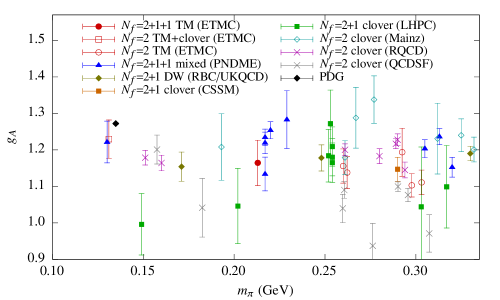
Figure 1: Axial charge versus pion mass, computed using $N_{f}=2$ and $N_{f}=2+1+1$ twisted mass fermions Alexandrou et al. (2014); a mixed action with clover-improved Wilson valence quarks and $N_{f}=2+1+1$ HISQ staggered sea quarks Gupta et al. (2014); $N_{f}=2+1$ domain wall fermions Ohta (2014a); $N_{f}=2+1$ clover-improved Wilson fermions, without Owen et al. (2013) and with Green et al. (2014b) smearing; and $N_{f}=2$ clover-improved Wilson fermions Jäger et al. (2014); Bali (2014); Horsley et al. (2014). Note that some of the same ensembles were used by RQCD and QCDSF, so that their errors may be correlated.

Obtaining agreement with the experimental value has proven difficult for lattice calculations. Those that include pion masses below 300 MeV are shown in Fig. 1. Note that, unless otherwise stated, the plotted data show the “raw” values from each lattice ensemble, renormalized but without any extrapolations to zero lattice spacing, infinite volume, or physical pion mass. In general, the lattice data tend to lie below the experimental value and show no strong dependence on the pion mass. In the past, the added uncertainty due to extrapolations to the physical pion mass meant that data that were below experiment could still be reconciled with it Edwards et al. (2006), but this becomes more difficult as calculations with near-physical pion masses become available.

The possibility of large excited-state contaminations affecting lattice calculations of $g_{A}$ has seen several studies in recent years. The Mainz group obtained agreement of their extrapolated value with experiment, when using the summation method to remove contributions from excited states, whereas the ratio method with a source-sink separation $T\approx 1.1$ fm produced a value below experiment Capitani et al. (2012). Using similar methods, LHPC reported similar results for pion masses $m_{\pi}\gtrsim 250$ MeV, but found that closer to the physical pion mass, removing excited states yielded even lower values of $g_{A}$ than typical lattice calculations Green et al. (2014b). Further evidence for the importance of excited-state effects comes from comparing results from the RQCD and QCDSF collaborations in Fig. 1, where many of the same lattice ensembles were used (thus controlling most systematics) but different quark-field smearing was used in the interpolating operator, leading to significantly different values of $g_{A}$ Collins et al. (2014).

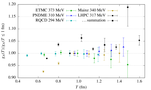
Figure 2: Axial charge, computed using the ratio method, versus source-sink separation $T$, with pion masses 373 Alexandrou et al. (2014), 310 Bhattacharya et al. (2014), 294 Collins et al. (2014), 340 Junnarkar et al. (2014), and 317 Green (2013) MeV. Data are normalized to their values at $T$ slightly below 1 fm. For the very-high-precision study from LHPC, we also show the summation-method results, computed using finite differences between the sums at the two nearest source-sink separations.

Some dedicated studies of excited-state effects are shown in Fig. 2. The highest-precision data are from a calculation by LHPC using very high statistics and a large volume; these indicate a $-5\%$ shift caused by excited states, when using the ratio method with a source-sink separation $T$ slightly below 1 fm. Other calculations have noisier results, but the dependence on $T$ past 1 fm is consistent with the LHPC data. On the other hand, studying Fig. 2 below $T=1$ fm, where excited-state effects are expected to be more prominent, shows different behaviour among the different calculations. This may indicate that ETMC and RQCD were more successful at tuning their interpolating operators to eliminate these effects. Finally, this figure also shows the effectiveness of the summation method at removing excited-state effects using relatively small source-sink separations, albeit with increased noise compared with the ratio method.

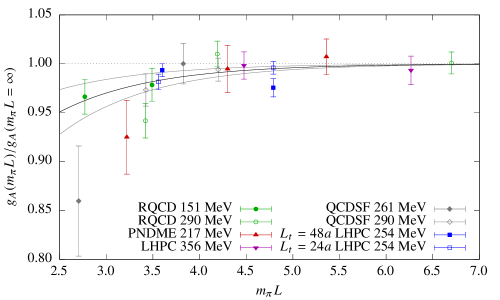
Figure 3: Axial charge versus the product of pion mass and spatial box length, $m_{\pi}L$, from RQCD Bali (2014), QCDSF Horsley et al. (2014), PNDME Gupta et al. (2014), and LHPC Bratt et al. (2010); Green et al. (2014c). Data are normalized to their infinite-volume extrapolation (see text), and the black and gray curves show the fitted dependence on $m_{\pi}L$ and its $1\sigma$ error. Note that the two calculations with $m_{\pi}=290$ MeV used the same two ensembles, so a 50% error correlation was assumed when fitting. At $m_{\pi}=254$ MeV, the spatial and temporal extents of the box were varied independently; here we treat the two temporal extents as two independent finite-volume studies.

The other major focus in studies of systematic errors for $g_{A}$ has been on the finite-volume effects, which have been prominently emphasized in works of the RBC-UKQCD collaboration, particularly in Ref. Yamazaki et al. (2008), where $g_{A}$ was found to depend significantly on $m_{\pi}L$, even in the region around $m_{\pi}L=4$, and that $m_{\pi}L\gtrsim 6$ would be needed to keep finite-volume effects below 1%. There have been relatively few fully-controlled studies of finite-volume effects. These are shown in Fig. 3, where we see that small volumes lead to small values of $g_{A}$. In order to study the dependence on the box size, we fit the data using a floating norm with a crude model,

$$g_{A}(m_{\pi}L,\dots)=A(\dots)(1+Be^{-m_{\pi}L}),$$ (8)

where $A(\dots)$ depends on all parameters except for $m_{\pi}L$. I.e., the data in Fig. 3 are fitted using eight independent parameters $A(\dots)$ and a universal $B$ parametrizing the finite-volume effects; then $A$ is used to normalize each dataset in the figure. Although the model isn’t a perfect description of the data ($\chi^{2}/\text{dof}=20/9$), it implies a small shift in the value of $g_{A}$ by $-1.1(5)\%$ when $m_{\pi}L=4$.

It should also be noted that we are neglecting any interactions between the box size and other systematic errors. For the case of excited states, this could be an important effect if significant contributions come from multi-particle $N\pi$ or $N\pi\pi$ states, since the energy gaps and couplings to the interpolating operator would depend on the box size. If we insist on controlling excited states before studying finite-volume effects, then the constraints that we can find on the latter are weaker; e.g., Ref. Green et al. (2014c) indicates that $g_{A}$ is shifted by less than 5% when $m_{\pi}L=4$.

At this point, there is no consensus, among those who perform lattice QCD calculations of nucleon structure, regarding a single culprit for the long-standing discrepancy with experimental measurements of $g_{A}$. The very recent ability to perform calculations at the physical pion mass will eliminate one source of uncertainty, but it seems that the axial charge will remain a troublesome observable for the near future. The problems may ultimately prove to come from a combination of multiple systematic errors, and it is possible that less-studied issues may be important, such as thermal states arising from a finite time-extent Green et al. (2014b) or inefficient sampling of gauge fields leading to a long-range autocorrelation Ohta (2014a).

2.2 Electromagnetic form factors

The Dirac and Pauli form factors of the vector current,

$$\langle p^{\prime}|\bar{q}\gamma^{\mu}q|p\rangle=\bar{u}(p^{\prime})\left(\gamma^{\mu}F_{1}^{q}(Q^{2})+\frac{i\sigma^{\mu\nu}(p^{\prime}-p)_{\nu}}{2m_{N}}F_{2}^{q}(Q^{2})\right)u(p),$$ (9)

where $Q^{2}=-(p^{\prime}-p)^{2}$, have been the primary off-forward benchmarks for lattice nucleon-structure calculations. The isovector ($u-d$) combination can be compared with the difference between proton and neutron form factors from elastic scattering with electrons, which are usually given in terms of electric and magnetic Sachs form factors,

$$G_{E}(Q^{2}) =F_{1}(Q^{2})-\frac{Q^{2}}{(2m_{N})^{2}}F_{2}(Q^{2}),$$ (10)

$$G_{M}(Q^{2}) =F_{1}(Q^{2})+F_{2}(Q^{2}).$$ (11)

As was the case for the axial charge, lattice calculations of the electromagnetic form factors have disagreed with experiment, producing a much milder dependence on $Q^{2}$. For a long time this was easily attributable to the use of heavier-than-physical pion masses, since chiral perturbation theory predicts that both the isovector charge and magnetic radii diverge in the chiral limit. However, this discrepancy persisted as pion masses were reduced.

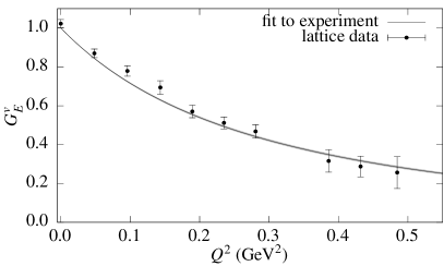
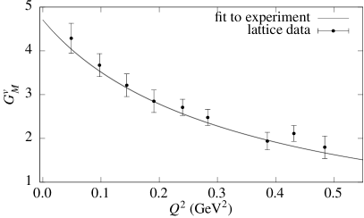
Figure 4: Isovector electromagnetic form factors. The lattice data are from the calculation in Refs. Green et al. (2014c, a), with $m_{\pi}=149$ MeV and using the summation method to reduce excited-state effects. The curves (including narrow error bands) are from the fit to experimental data in Ref. Alberico et al. (2009).

Studies of contributions from excited states have found large effects Green et al. (2011, 2014a); von Hippel et al. (2014); Koutsou et al. (2014), and that by reducing them and using relatively light pion masses, much of the gap between lattice calculations and experiment could be closed. This is displayed in Fig. 4, which shows results from a calculation where the isovector $G_{E}$ and $G_{M}$ agree with experiment Green et al. (2014c, a). Although this needs to be reproduced and successful control over excited states remains a significant challenge, these results are an encouraging sign of progress in nucleon structure calculations.

The behaviour of the form factors near $Q^{2}=0$ is of particular interest, as it yields the charge and magnetic radii ($r_{E}^{2}$ and $r_{M}^{2}$) and the magnetic moment $\mu$,

$$G_{E}(Q^{2}) =1-\frac{Q^{2}}{6}r_{E}^{2}+O(Q^{4}),$$ (12)

$$G_{M}(Q^{2}) =\mu\left(1-\frac{Q^{2}}{6}r_{M}^{2}+O(Q^{4})\right).$$ (13)

In particular, experimental determinations of the proton charge radius have a 7$\sigma$ discrepancy between the very precise value determined from spectroscopy of muonic hydrogen Antognini et al. (2013), $r_{E}^{p}=0.84087(39)$ fm, and the CODATA value determined from scattering and spectroscopy with electrons Mohr et al. (2012), $r_{E}^{p}=0.8775(51)$ fm. Having a reliable ab initio calculation of the proton charge radius (or even the isovector charge radius) is thus a highly attractive goal for practitioners of lattice QCD. Since the discrepancy in the squared proton charge radius $(r_{E}^{2})^{p}$ is 8–9%, even though lattice calculations are uncompetitive with the experimental precision, distinguishing between the two experimental values may be within reach in the next few years.

Given a form factor computed on the lattice, fitting is required to determine the radii and magnetic moment. This is usually done with a two-parameter dipole fit,

$$F(Q^{2})=\frac{F(0)}{\left(1+\frac{Q^{2}}{m_{D}^{2}}\right)^{2}},$$ (14)

although other forms have also been explored. Once form factors are reliably computed at the physical pion mass, this model-dependent fitting will probably be a leading source of uncertainty in radii and the magnetic moment. The situation could be improved with data at smaller $Q^{2}$; however, with periodic boundary conditions, the smallest available nonzero spatial momentum transfer is $2\pi/L_{s}$, so that even with the large $(5.6\text{ fm})^{3}$ volume used for the calculation shown in Fig. 4, the minimum momentum transfer was $Q^{2}=0.05\text{ GeV}^{2}$, an order of magnitude larger than obtained in scattering experiments Murphy et al. (1974); Simon et al. (1980); Bernauer et al. (2014).

We describe four strategies that might be used to obtain a better calculation of radii:

1. Use larger volumes to reduce $2\pi/L$ and thus the minimum $Q^{2}$. This is the most straightforward approach, and it is compatible with disconnected diagrams, so that the proton form factors could be directly computed. To access very low $Q^{2}$ without a rapid increase in computational costs, asymmetric boxes could be used, with one “long” spatial dimension.

2. Boost the source and sink nucleons to large momentum, in the direction of momentum transfer. This way, small $Q^{2}$ can be reached by increasing the energy difference between the source and the sink while keeping the spatial momentum transfer fixed to its minimum value. This strategy would likely require a nonstandard approach to the interpolating operators, since the usual smeared operators tend to have a poor signal and poor overlap with the ground state at large momentum Lin et al. (2010); Roberts et al. (2012); Della Morte et al. (2012).

3. Use (partially) twisted boundary conditions Bedaque (2004); de Divitiis et al. (2004); Sachrajda and Villadoro (2005). Using different boundary conditions on different quark flavors allow for arbitrary momentum transfer to be probed. The partially twisted case corresponds to only changing the boundary conditions on the valence quarks and not on the sea quarks, in order to reuse an existing ensemble of gauge configurations. However, twisted boundary conditions can introduce additional finite-volume effects that are exponentially suppressed at large volume, but may be significant in practice, especially for $F_{2}(Q^{2})$ Jiang and Tiburzi (2008); Tiburzi (2006). Since this technique relies on a transition between two flavors with different boundary conditions, it cannot be applied to disconnected diagrams, meaning that a clean, direct calculation of the proton form factors is not possible. There has been one preliminary study of the application of partially twisted boundary conditions to nucleon isovector form factors Hägler et al. (2008).

4. Use the Rome method de Divitiis et al. (2012). This amounts to setting up a calculation using partially twisted boundary conditions, and then analytically taking the derivative with respect to the twist angle, which requires computing additional sequential propagators. By evaluating the derivative at zero twist angle, momentum-derivatives of matrix elements at $Q^{2}=0$ can be computed, leading to a direct computation of the radii, independent of any fitting to $F(Q^{2})$. This has been studied for the pion in chiral perturbation theory Tiburzi (2014), where it was found that finite-volume effects for the charge radius asymptotically scale as $L^{1/2}e^{-m_{\pi}L}$. As with twisted boundary conditions, this method cannot be applied to disconnected diagrams.

Together with good control over excited states and the use of physical quark masses, these techniques may help to produce a reliable QCD calculation of the proton charge radius.

3 Other observables

3.1 Momentum fraction

The quark and gluon momentum fractions in a proton are obtained from forward matrix elements of the traceless energy-momentum tensor,

$$\langle p|T^{\mu\nu}_{q,g}|p\rangle=\langle x\rangle_{q,g}\bar{u}(p)\gamma^{\{\mu}p^{\nu\}}u(p),$$ (15)

where the braces denote taking the traceless symmetric part and

$$T^{\mu\nu}_{q} =\bar{q}\gamma^{\{\mu}i\overleftrightarrow{D}^{\nu\}}q,$$ (16)

$$T^{\mu\nu}_{g} =G^{\{\mu\alpha a}{G_{\alpha}}^{\nu\}a}.$$ (17)

These satisfy a sum rule: $\langle x\rangle_{g}+\sum_{q}\langle x\rangle_{q}=1$.

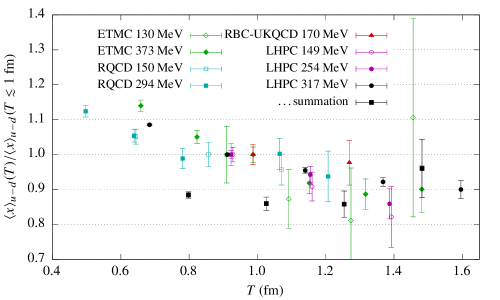
Figure 5: Isovector average quark momentum fraction, computed using the ratio method, versus source-sink separation $T$, with pion masses 130 and 373 Alexandrou et al. (2014), 150 and 294 Bali et al. (2014), 170 Ohta (2014b), 149 and 254 Green et al. (2014b), and 317 Green (2013) MeV. Data are normalized to their values at $T$ slightly below 1 fm. For the very-high-precision study from LHPC, we also show the summation-method results, computed using finite differences between the sums at the two nearest source-sink separations.

In order to avoid the need for disconnected diagrams, most calculations have been focussed on the isovector combination, $\langle x\rangle_{u-d}$. It has been found that this observable suffers from large excited-state effects; a selection of excited-state studies is shown in Fig. 5. These are broadly consistent with one another and indicate that using the ratio method with source-sink separation slightly below 1 fm yields a value 10–15% above the ground-state value, although the effect may grow at smaller pion masses Green et al. (2014b). It seems clear that good control over excited states is essential for the momentum fraction; indeed, the calculation of Ref. Green et al. (2014b), using the summation method to reduce their effect and extrapolating to the physical pion mass, found $\langle x\rangle_{u-d}=0.140(21)$ (in the $\overline{\text{MS}}$ scheme at 2 GeV), which is in agreement with the phenomenological value.

Going beyond the isovector combination, we note the study by $\chi$QCD in which the gluon and individual $u$, $d$, and $s$ quark contributions to the nucleon’s momentum were computed Deka et al. (2013), albeit using fairly heavy quark masses and a quenched ensemble. There also have been some other recent studies of $\langle x\rangle_{g}$, using quenched Horsley et al. (2012) and dynamical Wiese et al. (2014) fermions, and it is encouraging that reasonable statistical errors can be obtained. Some studies of the disconnected contributions to the quark momentum fraction will be briefly discussed in the later section on disconnected diagrams. These observables also face a more complicated pattern of renormalization, where the quark and gluon momentum fractions mix. The mixing coefficients have been studied perturbatively Glatzmaier and Liu (2014) but not yet nonperturbatively.

3.2 Scalar and tensor charges

The nucleon scalar charge $g_{S}$ and tensor charge $g_{T}$ are defined, analogously to the axial charge, via neutron-to-proton transition matrix elements:

$$\langle p(P)|\bar{u}d|n(P)\rangle =g_{S}\bar{u}_{p}(P)u_{n}(P),$$ (18)

$$\langle p(P)|\bar{u}\sigma^{\mu\nu}d|n(P)\rangle =g_{T}\bar{u}_{p}(P)\sigma^{\mu\nu}u_{n}(P).$$ (19)

In a study of generic beyond-the-Standard-Model contributions to neutron beta decay, it was shown that the leading effects are proportional to these two couplings; thus, calculations of $g_{S}$ and $g_{T}$ are required in order to find constraints on BSM physics from beta-decay experiments Bhattacharya et al. (2012).

The tensor charge is also equal to the isovector first moment of the proton’s transversity,

$$g_{T}=\langle 1\rangle_{\delta u-\delta d}.$$ (20)

Experimental measurements with good precision are planned at Jefferson Lab Dudek et al. (2012); therefore the tensor charge is an attractive target for testing predictions of lattice QCD.

The scalar charge is related via the Feynman-Hellmann theorem to the contribution from the difference in $u$ and $d$ quark masses to the neutron-proton mass splitting,

$$g_{S}=\frac{(m_{n}-m_{p})_{\text{QCD}}}{m_{d}-m_{u}}$$ (21)

(up to higher order isospin-breaking corrections), which also provides an indirect way of calculating the scalar charge using lattice QCD González-Alonso and Camalich (2014).

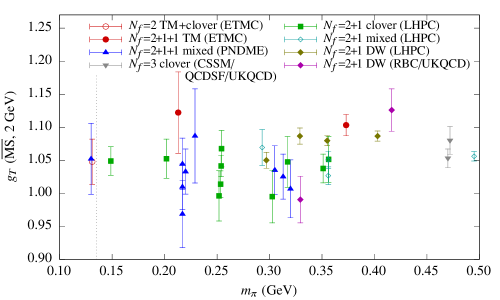
Figure 6: Nucleon tensor charge (renormalized in the $\overline{\text{MS}}$ scheme at 2 GeV) versus pion mass, computed using $N_{f}=2$ and $N_{f}=2+1+1$ twisted mass fermions Alexandrou et al. (2014), a mixed action with clover-improved Wilson valence quarks and $N_{f}=2+1+1$ HISQ staggered sea quarks Gupta et al. (2014), $N_{f}=3$ Zanotti et al. (2014) and $N_{f}=2+1$ Green et al. (2012a, b) clover-improved Wilson fermions with smearing, a mixed action with domain wall valence quarks and $N_{f}=2+1$ Asqtad staggered sea quarks Green et al. (2012a), and $N_{f}=2+1$ domain wall fermions Green et al. (2012a); Aoki et al. (2010). The vertical dotted line indicates the physical pion mass.

Lattice QCD calculations of the tensor charge are summarized in Fig. 6. There is no sign of a significant dependence on the pion mass. In addition, when excited-state effects have been studied for $g_{T}$, they have been found to be small Green et al. (2012a); Bhattacharya et al. (2014); Alexandrou et al. (2014), and the preliminary extrapolation in Ref. Gupta et al. (2014) to the continuum and infinite-volume limits found only mild effects. Thus the tensor charge appears to be a well-behaved observable, and should serve as a good test for lattice calculations when precise experimental measurements become available.

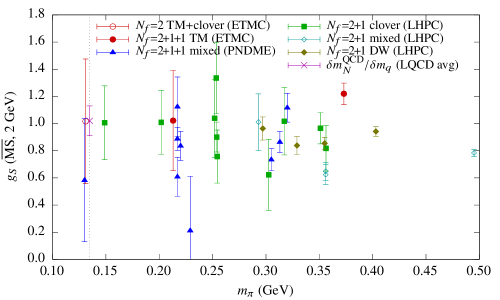
Figure 7: Nucleon scalar charge (renormalized in the $\overline{\text{MS}}$ scheme at 2 GeV) versus pion mass, computed using $N_{f}=2$ and $N_{f}=2+1+1$ twisted mass fermions Alexandrou et al. (2014), a mixed action with clover-improved Wilson valence quarks and $N_{f}=2+1+1$ HISQ staggered sea quarks Gupta et al. (2014), $N_{f}=2+1$ clover-improved Wilson fermions with smearing Green et al. (2012a, b), a mixed action with domain wall valence quarks and $N_{f}=2+1$ Asqtad staggered sea quarks Green et al. (2012a), $N_{f}=2+1$ domain wall fermions Green et al. (2012a), and indirectly using Eq. (21) with lattice QCD data at the physical point González-Alonso and Camalich (2014). The vertical dotted line indicates the physical pion mass.

Similarly, we show the scalar charge in Fig. 7. This suffers from considerably more noise than the axial and tensor charges; as a result, it is difficult to clearly identify systematic effects. ETMC reports large excited-state effects Alexandrou et al. (2014), but higher statistics are needed to confirm that this is a problem.

4 Disconnected diagrams

The disconnected-diagrams contributions to a hadron three-point function equal the correlation between a disconnected loop,

$$T(\vec{p}^{\prime}-\vec{p},\tau)=\sum_{\vec{y}}e^{i(\vec{p}^{\prime}-\vec{p})\cdot(\vec{y}-\vec{x}_{0})}\mathcal{O}(y,t_{0}+\tau),$$ (22)

and the hadron’s two-point function, Eq. (1). For a local quark bilinear operator, $\mathcal{O}=\bar{q}\Gamma q$, this requires computing the quark propagator from every point $y$ back to itself, $\operatorname{Tr}(\Gamma S[U](y,y))$, which is typically done using stochastic estimation by introducing noise vectors $\eta$ that have expectation value $E(\eta\eta^{\dagger})=I$. Solving $D[U]\psi=\eta$ yields a stochastic estimate for the all-to-all propagator, $S[U]=E(\psi\eta^{\dagger})$. Various techniques are used to reduce the noise associated with this procedure more efficiently than the $1/\sqrt{n}$ obtained by using many noise sources.

	ETMC Abdel-Rehim et al. (2014); Vaquero et al. (2014)	LHPC Meinel et al. (2014)	LANL Yoon et al. (2014)
$N_{f}$	$2+1+1$	$2+1$	$2+1+1$
Action	twisted mass	clover	clover on HISQ
$a$	0.082 fm	0.114 fm	0.12 fm
$m_{\pi}$	372 MeV	317 MeV	305 MeV
$N_{\text{samp}}(C_{\text{2pt}})$	147k	99k	61k
Methods	truncated solver Collins et al. (2007); Bali et al. (2010),	hierarchical probing Stathopoulos et al. (2013)	truncated solver,
for loops	one-end trick Michael and Urbach (2007)		hopping parameter expansion Collins et al. (2007); Bali et al. (2010)
$R(g_{A}^{u+d})$	$-0.12(2)$	$-0.12(2)$	$-0.19(2)$
$R(g_{T}^{u+d})$	$-0.002(2)$	$-0.005(10)$	$-0.039(8)$
$R(g_{S}^{u+d})$	$0.101(15)$	$1.756(94)$	$0.328(25)$
$R(\langle x\rangle_{u+d})$	$0.05(13)$	$0.24(4)$	—

Table 1: Recent calculations of light quark disconnected contributions to isoscalar nucleon forward matrix elements. $R(X)$ is defined as the ratio of disconnected to connected contributions to the observable $X$.

There are an increasing number of nucleon-structure calculations that include disconnected diagrams, however these generally do not cover the same range of ensembles as for connected diagrams, so that less is known about systematic errors. Three such calculations that were presented at the Lattice 2014 conference, covering a range of observables, are shown in Tab. 1. These used $O(10^{5})$ samples of the two-point function in order to obtain a good signal (cf. typically $10^{3}$–$10^{4}$ samples for connected three-point functions), along with various stochastic-estimation techniques for the disconnected loops. The importance of disconnected contributions is highly observable-dependent: they form a moderate positive contribution to the isoscalar scalar charge (relevant for the nucleon sigma term) and momentum fraction, a moderate negative contribution to the isoscalar axial charge, and a small contribution to the isoscalar tensor charge.

For the light-quark disconnected contribution to electromagnetic form factors, a clear nonzero signal was found by LHPC Meinel et al. (2014). For the proton $G_{E}$ and $G_{M}$, these were less than 1% of the connected part (positive for $G_{E}$, negative for $G_{M}$). This calculation made use of hierarchical probing, an approach that eliminates the variance of $\eta(x)\eta^{\dagger}(y)$ for nearby spatial sites $x$ and $y$, and was found to be particularly effective at reducing the noise for the vector current.

These calculations are still in their infancy for most nucleon observables: the pion mass dependence and other systematics have not been probed. But these first calculations are a promising sign that reasonable signals can be obtained using existing techniques.

5 Conclusions

Lattice QCD calculations of nucleon structure have been making steady progress toward full control over systematic errors. The ability to calculate using the physical pion mass will nearly eliminate the uncertainty associated with chiral extrapolation. Excited-state contamination has been identified as an important source of errors, and due to the exponentially-decaying signal, removing it remains a challenge.

The axial charge remains the primary “benchmark” observable for nucleon structure calculations, and agreement with experiment remains problematic — even in the cases where agreement within errors was obtained, the lattice values are mostly below the experimental value, rather than scattered on both sides of it. Until this issue is unambiguously resolved, predictions of other observables will likely have to be treated with some caution.

For electromagnetic form factors, it appears that the approach to the physical pion mass and the removal of excited-state effects are the most important systematics to control. It is promising that a calculation has produced agreement with the experimental form factors, and that a good signal has been obtained for the disconnected contribution. The application of new techniques to probe the form factors at low $Q^{2}$ may help to produce a solid first-principles calculation of the proton charge radius with sufficient accuracy to discriminate between the two experimental values.

The same methodology is being applied to observables such as the quark and gluon momentum fractions, and the scalar and tensor charges. The sources of uncertainty vary significantly: excited states are significant for the momentum fraction, whereas statistical fluctuations are quite large for the scalar charge. The tensor charge appears to be under reasonably good control, and the agreement among lattice calculations that its value is around 1.05 will provide a good test once it is measured experimentally.

6 Acknowledgments

I thank John Negele for comments on a draft of this review as well as my other collaborators in LHPC for their invaluable contributions to some of the work presented here: Michael Engelhardt, Stefan Krieg, Stefan Meinel, Andrew Pochinsky, and Sergey Syritsyn. I am also grateful to my colleagues at Mainz for their helpful comments on an early version of this talk.

References

- Aoki et al. (2014) S. Aoki, Y. Aoki, C. Bernard, T. Blum, G. Colangelo, et al., Eur. Phys. J. C 74, 2890 (2014), 1310.8555.
- Lepage (1989) G. P. Lepage, “The Analysis of Algorithms for Lattice Field Theory,” in From Actions to Answers: Proceedings of the 1989 Theoretical Advanced Study Institute in Elementary Particle Physics, 5–30 June 1989, University of Colorado, Boulder, edited by T. DeGrand, and D. Toussaint, World Scientific, Singapore, 1989, pp. 97–120.
- Capitani et al. (2010) S. Capitani, B. Knippschild, M. Della Morte, and H. Wittig, PoS LATTICE2010, 147 (2010), 1011.1358.
- Bulava et al. (2010) J. Bulava, M. A. Donnellan, and R. Sommer, PoS LATTICE2010, 303 (2010), 1011.4393.
- Green et al. (2011) J. Green, J. Negele, A. Pochinsky, S. Krieg, and S. Syritsyn, PoS LATTICE2011, 157 (2011), 1111.0255.
- Bhattacharya et al. (2014) T. Bhattacharya, S. D. Cohen, R. Gupta, A. Joseph, H.-W. Lin, et al., Phys. Rev. D 89, 094502 (2014), 1306.5435.
- Collins et al. (2014) S. Collins, G. S. Bali, B. Gläßle, M. Göckeler, J. Najjar, et al., PoS LATTICE2013, 290 (2014), 1311.7041.
- Bali et al. (2014) G. S. Bali, S. Collins, B. Gläßle, M. Göckeler, J. Najjar, et al., Phys. Rev. D 90, 074510 (2014), 1408.6850.
- Alexandrou et al. (2014) C. Alexandrou, M. Constantinou, K. Hadjiyiannakou, K. Jansen, C. Kallidonis, et al., PoS LATTICE2014, 151 (2014), 1411.3494.
- von Hippel et al. (2014) G. M. von Hippel, S. Capitani, D. Djukanovic, J. Hua, B. Jäger, et al., PoS LATTICE2014, 147 (2014), 1411.4804.
- Junnarkar et al. (2014) P. M. Junnarkar, S. Capitani, D. Djukanovic, G. von Hippel, J. Hua, et al., PoS LATTICE2014, 150 (2014), 1411.5828.
- Aubin and Orginos (2011) C. Aubin, and K. Orginos, AIP Conf. Proc. 1374, 621–624 (2011), 1010.0202.
- Owen et al. (2013) B. J. Owen, J. Dragos, W. Kamleh, D. B. Leinweber, M. S. Mahbub, et al., Phys. Lett. B 723, 217–223 (2013), 1212.4668.
- Owen et al. (2014) B. J. Owen, W. Kamleh, D. B. Leinweber, M. S. Mahbub, and B. J. Menadue, PoS LATTICE2013, 277 (2014), 1312.0291.
- Green et al. (2014a) J. R. Green, J. W. Negele, A. V. Pochinsky, S. N. Syritsyn, M. Engelhardt, et al., Phys. Rev. D 90, 074507 (2014a), 1404.4029.
- Green et al. (2014b) J. R. Green, M. Engelhardt, S. Krieg, J. W. Negele, A. V. Pochinsky, et al., Phys. Lett. B 734, 290–295 (2014b), 1209.1687.
- Syritsyn et al. (2014) S. Syritsyn, T. Blum, M. Engelhardt, J. Green, T. Izubuchi, et al., PoS LATTICE2014, 134 (2014), 1412.3175.
- Koutsou et al. (2014) G. Koutsou, et al., PoS LATTICE2014, 148 (2014).
- Gupta et al. (2014) R. Gupta, et al., PoS LATTICE2014, 152 (2014).
- Collins et al. (2007) S. Collins, G. Bali, and A. Schäfer, PoS LATTICE2007, 141 (2007), 0709.3217.
- Bali et al. (2010) G. S. Bali, S. Collins, and A. Schäfer, Comput. Phys. Commun. 181, 1570–1583 (2010), 0910.3970.
- Blum et al. (2013) T. Blum, T. Izubuchi, and E. Shintani, Phys. Rev. D 88, 094503 (2013), 1208.4349.
- Lin (2014) M. Lin, PoS LATTICE2013, 275 (2014), 1401.1476.
- Ohta (2014a) S. Ohta, PoS LATTICE2014, 149 (2014a), 1410.8353.
- Olive et al. (2014) K. Olive, et al., Chin. Phys. C 38, 090001 (2014).
- Jäger et al. (2014) B. Jäger, T. D. Rae, S. Capitani, M. Della Morte, D. Djukanovic, et al., PoS LATTICE2013, 272 (2014), 1311.5804.
- Bali (2014) G. Bali, PoS LATTICE2014, 136 (2014).
- Horsley et al. (2014) R. Horsley, Y. Nakamura, A. Nobile, P. E. L. Rakow, G. Schierholz, et al., Phys. Lett. B 732, 41–48 (2014), 1302.2233.
- Edwards et al. (2006) R. G. Edwards, et al., Phys. Rev. Lett. 96, 052001 (2006), hep-lat/0510062.
- Capitani et al. (2012) S. Capitani, M. Della Morte, G. von Hippel, B. Jäger, A. Jüttner, et al., Phys. Rev. D 86, 074502 (2012), 1205.0180.
- Green (2013) J. R. Green, Studies in hadron structure using lattice QCD with quark masses that almost reach the physical point, Ph.D. thesis, Massachusetts Institute of Technology (2013), URL http://hdl.handle.net/1721.1/84184.
- Bratt et al. (2010) J. D. Bratt, et al., Phys. Rev. D 82, 094502 (2010), 1001.3620.
- Green et al. (2014c) J. Green, M. Engelhardt, S. Krieg, S. Meinel, J. Negele, et al., PoS LATTICE2013, 276 (2014c), 1310.7043.
- Yamazaki et al. (2008) T. Yamazaki, et al., Phys. Rev. Lett. 100, 171602 (2008), 0801.4016.
- Alberico et al. (2009) W. M. Alberico, S. M. Bilenky, C. Giunti, and K. M. Graczyk, Phys. Rev. C 79, 065204 (2009), 0812.3539.
- Antognini et al. (2013) A. Antognini, F. Nez, K. Schuhmann, F. D. Amaro, F. Biraben, et al., Science 339, 417–420 (2013).
- Mohr et al. (2012) P. J. Mohr, B. N. Taylor, and D. B. Newell, Rev. Mod. Phys. 84, 1527–1605 (2012), 1203.5425.
- Murphy et al. (1974) J. J. Murphy, Y. Shin, and D. M. Skopik, Phys. Rev. C 9, 2125–2129 (1974).
- Simon et al. (1980) G. G. Simon, C. Schmitt, F. Borkowski, and V. H. Walther, Nucl. Phys. A 333, 381–391 (1980).
- Bernauer et al. (2014) J. C. Bernauer, et al., Phys. Rev. C 90, 015206 (2014), 1307.6227.
- Lin et al. (2010) H.-W. Lin, S. D. Cohen, R. G. Edwards, K. Orginos, and D. G. Richards (2010), 1005.0799.
- Roberts et al. (2012) D. S. Roberts, W. Kamleh, D. B. Leinweber, M. S. Mahbub, and B. J. Menadue, Phys. Rev. D 86, 074504 (2012), 1206.5891.
- Della Morte et al. (2012) M. Della Morte, B. Jäger, T. Rae, and H. Wittig, Eur. Phys. J. A 48, 139 (2012), 1208.0189.
- Bedaque (2004) P. F. Bedaque, Phys. Lett. B 593, 82–88 (2004), nucl-th/0402051.
- de Divitiis et al. (2004) G. M. de Divitiis, R. Petronzio, and N. Tantalo, Phys. Lett. B 595, 408–413 (2004), hep-lat/0405002.
- Sachrajda and Villadoro (2005) C. T. Sachrajda, and G. Villadoro, Phys. Lett. B 609, 73–85 (2005), hep-lat/0411033.
- Jiang and Tiburzi (2008) F.-J. Jiang, and B. C. Tiburzi, Phys. Rev. D 78, 114505 (2008), 0810.1495.
- Tiburzi (2006) B. C. Tiburzi, Phys. Lett. B 641, 342–349 (2006), hep-lat/0607019.
- Hägler et al. (2008) P. Hägler, M. Göckeler, R. Horsley, Y. Nakamura, M. Ohtani, et al., PoS LATTICE2008, 138 (2008).
- de Divitiis et al. (2012) G. M. de Divitiis, R. Petronzio, and N. Tantalo, Phys. Lett. B 718, 589–596 (2012), 1208.5914.
- Tiburzi (2014) B. C. Tiburzi, Phys. Rev. D 90, 054508 (2014), 1407.4059.
- Ohta (2014b) S. Ohta, PoS LATTICE2013, 274 (2014b), 1309.7942.
- Deka et al. (2013) M. Deka, T. Doi, Y. Yang, B. Chakraborty, S. J. Dong, et al. (2013), 1312.4816.
- Horsley et al. (2012) R. Horsley, et al., Phys. Lett. B 714, 312–316 (2012), %****␣hadronstructure.bbl␣Line␣225␣****1205.6410.
- Wiese et al. (2014) C. Wiese, C. Alexandrou, V. Drach, K. Hadjiyiannakou, K. Jansen, et al., PoS LATTICE2013, 289 (2014), 1311.3174.
- Glatzmaier and Liu (2014) M. Glatzmaier, and K.-F. Liu (2014), 1403.7211.
- Bhattacharya et al. (2012) T. Bhattacharya, V. Cirigliano, S. D. Cohen, A. Filipuzzi, M. Gonzalez-Alonso, et al., Phys. Rev. D 85, 054512 (2012), 1110.6448.
- Dudek et al. (2012) J. Dudek, R. Ent, R. Essig, K. S. Kumar, C. Meyer, et al., Eur. Phys. J. A 48, 187 (2012), 1208.1244.
- González-Alonso and Camalich (2014) M. González-Alonso, and J. M. Camalich, Phys. Rev. Lett. 112, 042501 (2014), 1309.4434.
- Zanotti et al. (2014) J. Zanotti, et al., PoS LATTICE2014, 165 (2014).
- Green et al. (2012a) J. R. Green, J. W. Negele, A. V. Pochinsky, S. N. Syritsyn, M. Engelhardt, et al., Phys. Rev. D 86, 114509 (2012a), 1206.4527.
- Green et al. (2012b) J. Green, M. Engelhardt, S. Krieg, J. Negele, A. Pochinsky, et al., PoS LATTICE2012, 170 (2012b), 1211.0253.
- Aoki et al. (2010) Y. Aoki, T. Blum, H.-W. Lin, S. Ohta, S. Sasaki, et al., Phys. Rev. D 82, 014501 (2010), 1003.3387.
- Abdel-Rehim et al. (2014) A. Abdel-Rehim, C. Alexandrou, M. Constantinou, V. Drach, K. Hadjiyiannakou, et al., Phys. Rev. D 89, 034501 (2014), 1310.6339.
- Vaquero et al. (2014) A. Vaquero, C. Alexandrou, M. Constantinou, V. Drach, K. Hadjiyiannakou, et al., PoS LATTICE2014, 140 (2014), 1410.8761.
- Meinel et al. (2014) S. Meinel, et al., PoS LATTICE2014, 139 (2014).
- Yoon et al. (2014) B. Yoon, et al., PoS LATTICE2014, 141 (2014).
- Stathopoulos et al. (2013) A. Stathopoulos, J. Laeuchli, and K. Orginos (2013), 1302.4018.
- Michael and Urbach (2007) C. Michael, and C. Urbach, PoS LATTICE2007, 122 (2007), 0709.4564.