Low-energy excitations and quasielastic contribution to electron-nucleus and neutrino-nucleus scattering in the continuum random phase approximation

Abstract

We present a detailed study of a continuum random phase approximation approach to quasielastic electron-nucleus and neutrino-nucleus scattering. We compare the ($e,e^{\prime}$) cross-section predictions with electron scattering data for the nuclear targets ¹²C, ¹⁶O, and ⁴⁰Ca, in the kinematic region where quasielastic scattering is expected to dominate. We examine the longitudinal and transverse contributions to ¹²C($e,e^{\prime}$) and compare them with the available data. We find an overall satisfactory description of the ($e,e^{\prime}$) data. Further, we study the ¹²C($\nu_{\mu},\mu^{-}$) cross sections relevant for accelerator-based neutrino-oscillation experiments. We pay special attention to low-energy excitations which can account for non-negligible contributions in measurements, and require a beyond-Fermi-gas formalism.

I Introduction

The quest for a completion of our knowledge of neutrino-oscillation parameters has made tremendous progress in recent years. Still, neutrino-oscillation experiments face a number of challenges. Major issues are the identification of the basic processes contributing to the neutrino-nucleus signal in a detector and the reduction of the systematic uncertainties. A thorough understanding of the complexity of the nuclear environment and its electroweak response at low and intermediate energies is required. Charged-current quasielastic (CCQE) processes account for a large share of the detected signals in many experiments. Although several cross section measurements have been performed  miniboone:ccqenu ; miniboone:ccqeantinu ; miniboone:nunc ; minerva:nu ; minerva:antinu ; t2k:qenu ; t2k:qenu2 , uncertainties connected to the electroweak responses persist rev:Morfin ; rev:Nieves .

Despite substantial progress in the understanding of the different processes involved in the signal of neutrino-oscillation experiments, the simulation codes are primarily based on a Fermi-gas description of the nucleus. Relativistic Fermi-gas (RFG) based models are employed in Monte Carlo event generators. The RFG model provides a basic picture of the nucleus as a system of quasifree nucleons and takes into account the Fermi motion and Pauli blocking effects. The analysis of electron-scattering data suggests that at momentum transfers $q\approx$ 500 MeV/c, the RFG model describes the general behavior of the quasielastic (QE) cross section sufficiently accurately, but its description becomes poor for smaller momentum transfers, where nuclear effects are more prominent. Since the neutrino flux in the oscillation experiments is distributed over energies from very low to a few GeV, the cross section picks up contributions from all energies. The low excitation-energy cross sections do not receive proper attention in an RFG description. Furthermore, even at higher incoming neutrino energy, the contributions stemming from low transferred energies are not negligible. At low energy transfers, the nuclear structure certainly needs a beyond RFG description. Several studies emphasizing the low energy excitation in the framework of neutrino-nuclear interactions Kolbe:1995 ; Volpe:2000 ; Co:2005 ; Martini:2007 ; Samana:2011 have been performed. Those studies, however, have not been explicitly extended to explore the kinematics of MiniBooNE MiniBooNE , T2K T2K , and other similar experiments.

In this paper, we present a continuum random phase approximation (CRPA) approach for the description of QE electroweak scattering off the nucleus, crucial for accelerator-based neutrino-oscillation experiments. We pay special attention to low-energy nuclear excitations. In this context, the availability of a large amount of high-precision electron-nucleus scattering data is of the utmost importance, as it allows one to test the reliability of the reaction model.

Several models have been developed to study electron-nucleus scattering and further generalized to describe neutrino-nucleus cross sections Alberico:1982 ; Martini:2009 ; Martini:2013 ; Nieves:1997 ; Nieves:2004 ; Nieves:2005 ; Benhar:1994 ; Benhar:2005 ; Benhar:2007 ; Ankowski:2014 ; Amaro:2005 ; Amaro:2007 ; Mosel:2009 ; Butkevich:2005 ; Butkevich:2007 ; Meucci:2003 ; Meucci:2004 ; Co:1984 . An extensive test against the inclusive quasielastic electron scattering is performed within an RFG and plane-wave impulse approximation approach in Ref. Butkevich:2005 , while a spectral function based approach is assessed in Ref. Ankowski:2014 . The model we adopt takes a Hartree-Fock (HF) description of nuclear dynamics as a starting point and additionally implements long-range correlations through a CRPA framework with an effective Skyrme nucleon-nucleon two-body interaction. We solve the CRPA equations by a Green’s function approach. Thereby, the polarization propagator is approximated by an iteration of its first-order contribution. In this way, the formalism implements the description of one-particle one-hole excitations out of the correlated nuclear ground state. To improve our description of the kinematics of the interaction at intermediate energies, we implemented an effective relativistic approach proposed in Refs. Donnelly:1998 ; Amaro:2005 ; Amaro:2007 .

The article is organized as follows. In Sec. II, we outline the details of the QE electron and neutrino-nucleus cross-section formalism. We describe the CRPA framework for calculating nuclear responses. Sec. III, is divided into two parts: In Sec. III.1, we present numerical results of electron-scattering cross sections (on a variety of nuclear targets), and responses (on ¹²C) and compare them with the available data. In Sec. III.2, we discuss neutrino-scattering results in the context of accelerator-based neutrino-oscillation experiments. We pay special attention to low-energy neutrino-induced nuclear excitations. Conclusions can be found in Sec. IV.

II Formalism

In this section, we describe our CRPA-based approach for the calculation of the nuclear response for inclusive electron and neutrino-nucleus scattering in the QE region. This approach was successful in describing exclusive photo-induced and electron-induced QE processes Jan:1988 ; Jan:1989 , and inclusive neutrino scattering at supernova energies Natalie:nc1999 ; Natalie:cc2002 ; Natalie:nc2004 ; Natalie:sn2006 ; Natalie:proc2009 ; Natalie:nuintproc2012 . We have also used this approach to calculate the inclusive CCQE antineutrino-nucleus scattering cross sections at intermediate energies Vishvas:ccqeantinu2014 . Here, we are using an updated version of the same formalism.

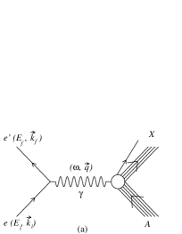
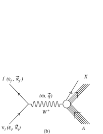
Figure 1: Inclusive processes considered in this paper: (a) QE electron-nucleus and (b) CCQE neutrino-nucleus ($l=e,\mu,\tau$), where $X$ is the undetected hadronic final state.

We consider QE electron and CCQE neutrino scattering off a nucleus under conditions where the details of the final hadron state remain unobserved. As shown in Fig. 1, an incident electron (neutrino) with four-momentum $E_{i},\vec{k}_{i}$ ($\varepsilon_{i},\vec{\kappa}_{i}$) scatters off a nucleus via the exchange of a photon ($W$-boson) and only the outgoing charged lepton with four-momentum $E_{f},\vec{k}_{f}$ ($\varepsilon_{f},\vec{\kappa}_{f}$) is detected in the final state

$$e(E_{i},\vec{k}_{i})+A\rightarrow e^{\prime}(E_{f},\vec{k}_{f})+X,$$ (1)

and

$$\nu_{l}(\varepsilon_{i},\vec{\kappa}_{i})+A\rightarrow l^{-}(\varepsilon_{f},\vec{\kappa}_{f})+X,$$ (2)

where $l$ represents $e$, $\mu$, or $\tau$. Further, $A$ is the nucleus in its ground state $|J_{i},M_{i}\rangle$ and $X$ is the unobserved hadronic final state.

The double differential cross section for electron and neutrino-nucleus scattering of Eqs. (1) and  (2) can be expressed as

$$\left(\frac{d^{2}\sigma}{d{\omega}d{\Omega}}\right)_{e}~{}=~{}\frac{\alpha^{2}}{Q^{4}}~{}\left(\frac{2}{2J_{i}+1}\right)~{}E_{f}k_{f}\cos^{2}(\theta/2)$$

$$~{}~{}~{}~{}~{}~{}~{}~{}\times~{}\zeta^{2}\left(Z^{\prime},E_{f},q\right)~{}\left[\sum_{J=0}^{\infty}\sigma_{L,e}^{J}+\sum_{J=1}^{\infty}\sigma_{T,e}^{J}\right],$$ (3)

and

$$\left(\frac{d^{2}\sigma}{d{\omega}d{\Omega}}\right)_{\nu}~{}=~{}\frac{G_{F}^{2}~{}\cos^{2}{\theta_{c}}}{(4\pi)^{2}}~{}\left(\frac{2}{2J_{i}+1}\right)~{}\varepsilon_{f}{{\kappa}_{f}}$$

$$~{}~{}~{}~{}~{}~{}\times~{}\zeta^{2}\left(Z^{\prime},\varepsilon_{f},q\right)~{}\left[\sum_{J=0}^{\infty}\sigma_{CL,\nu}^{J}+\sum_{J=1}^{\infty}\sigma_{T,\nu}^{J}\right],$$ (4)

where $\alpha$ is the fine-structure constant, $G_{F}$ is the Fermi coupling constant, and $\theta_{c}$ is the Cabibbo angle. The direction of the outgoing lepton is described by the solid angle $\Omega$. The lepton-scattering angle is $\theta$, the transferred four-momentum is $q^{\mu}(\omega,\vec{q})$ and $Q^{2}=-q_{\mu}q^{\mu}$. Further, $\zeta(Z^{\prime},E,q)$ is introduced in order to take into account the distortion of the lepton wave function in the Coulomb field generated by $Z^{\prime}$ protons, within a modified effective momentum approximation Engel:1998 .

The $\sigma_{L,e}^{J}$ ($J$ denotes the multipole number) and $\sigma_{T,e}^{J}$ are the longitudinal and transverse components of the electron-nucleus scattering cross section, while $\sigma_{CL,\nu}^{J}$ and $\sigma_{T,\nu}^{J}$ are the Coulomb-longitudinal and transverse contributions of the neutrino-nucleus scattering cross section. In Fig. 2, we plot the strength obtained by adding the different multipole contributions to the cross section for incident neutrino energies from 0.1 to 2.0 GeV. Naturally, the higher the energy of the incident particle, the more multipoles contribute to the cross section. From the figure, one observes that for energies as low as 200 MeV, multipoles up to $J=$ 4 contribute. For energies as high as 2 GeV, multipoles up to $J=$16 need to be considered, and the relative weight of small $J$ contributions diminishes.

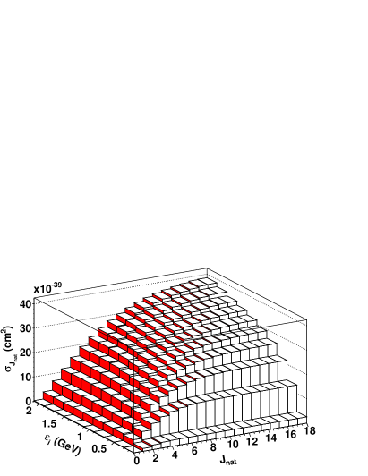
Figure 2: (Color online) Multipole contributions (for natural parity transitions) to the cross section, as a function of the incoming neutrino energy. The $\sigma_{J_{nat}}$ denotes the ¹²C$(\nu_{\mu},\mu^{-})$ cross section including all multipoles of the natural parity excitations up to $J_{nat}$.

The (Coulomb) longitudinal and transverse parts of the cross section both are composed of a kinematical factor $(v)$ and a response function $(R)$. The response function contains the full nuclear structure information. In the electron scattering case, the longitudinal ($\sigma_{L,e}$) and transverse ($\sigma_{T,e}$) components of the cross section can be expressed as follows

$$\sigma_{L,e}=v^{L}_{e}R^{L}_{e},~{}~{}~{}\sigma_{T,e}=v^{T}_{e}R^{T}_{e},$$ (5)

where the leptonic factors, $v^{L}_{e}$ and $v^{T}_{e}$, are given by

$$v^{L}_{e}=\frac{Q^{4}}{|\vec{q}|^{4}},~{}~{}~{}v^{T}_{e}=\left[\frac{Q^{2}}{2|\vec{q}|^{2}}~{}+~{}\tan^{2}(\theta/2)\right].$$ (6)

Longitudinal $R^{L}_{e}$ and transverse $R^{T}_{e}$ response functions are defined as

$$R^{L}_{e}=|\langle J_{f}||\widehat{\mathcal{M}}_{J}^{e}(|\vec{q}|)||J_{i}\rangle|^{2},$$ (7)

$$R^{T}_{e}=\left[|\langle J_{f}||\widehat{\mathcal{J}}_{J}^{mag,e}(|\vec{q}|)||J_{i}\rangle|^{2}+|\langle J_{f}||\widehat{\mathcal{J}}_{J}^{el,e}(|\vec{q}|)||J_{i}\rangle|^{2}\right].$$

Here $\widehat{\mathcal{M}}_{J}^{e}$, ${\widehat{\mathcal{J}}}_{J}^{mag,e}$ and ${\widehat{\mathcal{J}}}_{J}^{el,e}$ are the longitudinal, transverse magnetic and transverse electric operators, respectively Connell:1972 ; Walecka:1995 . The $|J_{i}\rangle$ and $|J_{f}\rangle$ denote the initial and final state of the nucleus.

Similarly for neutrino-scattering processes, we express the Coulomb-longitudinal ($\sigma_{CL,\nu}$) and transverse ($\sigma_{T,\nu}$) parts of the cross section as follows:

$$\sigma_{CL,\nu} = \left[v^{\mathcal{M}}_{\nu}R^{\mathcal{M}}_{\nu}+v^{\mathcal{L}}_{\nu}R^{\mathcal{L}}_{\nu}+~{}2~{}v^{\mathcal{M}\mathcal{L}}_{\nu}R^{\mathcal{M}\mathcal{L}}_{\nu}\right],$$ (9)

$$\sigma_{T,\nu} = \left[v^{T}_{\nu}R^{T}_{\nu}+2~{}v^{TT}_{\nu}R^{TT}_{\nu}\right],$$ (10)

where leptonic coefficients $v^{\mathcal{M}}_{\nu}$, $v^{\mathcal{L}}_{\nu}$, $v^{\mathcal{M\mathcal{L}}}_{\nu}$, $v^{T}_{\nu}$, and $v^{TT}_{\nu}$ are given as

$$v^{\mathcal{M}}_{\nu}=\left[1+\frac{\kappa_{f}}{\varepsilon_{f}}\cos\theta\right],$$ (11)

$$v^{\mathcal{L}}_{\nu}=\left[1+\frac{\kappa_{f}}{\varepsilon_{f}}\cos\theta-\frac{2\varepsilon_{i}\varepsilon_{f}}{|\vec{q}|^{2}}{\left(\frac{\kappa_{f}}{\varepsilon_{f}}\right)}^{2}\sin^{2}\theta\right],$$ (12)

$$v^{\mathcal{M}\mathcal{L}}_{\nu}=\left[\frac{\omega}{|\vec{q}|}\left(1+\frac{\kappa_{f}}{\varepsilon_{f}}\cos\theta\right)+\frac{m_{l}^{2}}{\varepsilon_{f}|\vec{q}|}\right],$$ (13)

$$v^{T}_{\nu}=\left[1-\frac{\kappa_{f}}{\varepsilon_{f}}\cos\theta+\frac{\varepsilon_{i}\varepsilon_{f}}{|\vec{q}|^{2}}{\left(\frac{\kappa_{f}}{\varepsilon_{f}}\right)}^{2}\sin^{2}\theta\right],$$ (14)

$$v^{TT}_{\nu}=\left[\frac{\varepsilon_{i}+\varepsilon_{f}}{|\vec{q}|}\left(1-\frac{\kappa_{f}}{\varepsilon_{f}}\cos\theta\right)-\frac{m_{l}^{2}}{\varepsilon_{f}|\vec{q}|}\right],$$ (15)

and response functions $R^{\mathcal{M}}_{\nu}$, $R^{\mathcal{L}}_{\nu}$, $R^{\mathcal{ML}}_{\nu}$, $R^{T}_{\nu}$, and $R^{TT}_{\nu}$ are defined as

$$R^{\mathcal{M}}_{\nu}=|\langle J_{f}||\widehat{\mathcal{M}}_{J}^{\nu}(|\vec{q}|)||J_{i}\rangle|^{2},$$ (16)

$$R^{\mathcal{L}}_{\nu}=|\langle J_{f}||\widehat{\mathcal{L}}_{J}^{\nu}(|\vec{q}|)||J_{i}\rangle|^{2},$$ (17)

$$R^{\mathcal{ML}}_{\nu}=~{}\mathcal{R}\left[\langle J_{f}||\widehat{\mathcal{L}}_{J}^{\nu}(|\vec{q}|)||J_{i}\rangle\langle J_{f}||\widehat{\mathcal{M}}_{J}^{\nu}(|\vec{q}|)||J_{i}\rangle^{\ast}\right],$$ (18)

$$R^{T}_{\nu}=\left[|\langle J_{f}||\widehat{\mathcal{J}}_{J}^{mag,\nu}(|\vec{q}|)||J_{i}\rangle|^{2}+|\langle J_{f}||\widehat{\mathcal{J}}_{J}^{el,\nu}(|\vec{q}|)||J_{i}\rangle|^{2}\right],$$

$$R^{TT}_{\nu}=~{}\mathcal{R}\left[\langle J_{f}||\widehat{\mathcal{J}}_{J}^{mag,\nu}(|\vec{q}|)||J_{i}\rangle\langle J_{f}||\widehat{\mathcal{J}}_{J}^{el,\nu}(|\vec{q}|)||J_{i}\rangle^{\ast}\right].$$

Here $\widehat{\mathcal{M}}_{J}^{\nu}$, $\widehat{\mathcal{L}}_{J}^{\nu}$, $\widehat{\mathcal{J}}_{J}^{mag,\nu}$ and $\widehat{\mathcal{J}}_{J}^{el,\nu}$ are the Coulomb, longitudinal, transverse magnetic, and transverse electric operators, respectively Connell:1972 ; Walecka:1995 .

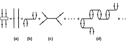
Figure 3: Diagrammatic representation of the polarization propagator $\Pi^{(RPA)}$ for particle-hole states. Panel (a) corresponds to the unperturbed polarization propagator $\Pi^{(0)}$, (b) and (c) are the first-order direct and exchange RPA diagrams, and (d) represents a typical higher-order RPA diagram.

To calculate the nuclear response functions, we use the CRPA approach which is described in detail in Refs. Jan:1988 ; Jan:1989 ; Natalie:nc1999 ; Natalie:cc2002 . Here we will briefly present the essence of our model. We start by describing the nucleus within a mean-field (MF) approximation. The MF potential is obtained by solving the Hartree-Fock (HF) equations with a Skyrme (SkE2) two-body interaction Jan:1988 ; Jan:1989 . The sequential filling of the single-nucleon orbits automatically introduces Pauli-blocking. The continuum wave functions are obtained by integrating the positive-energy Schrödinger equation with appropriate boundary conditions. In this manner, we account for the final-state interactions of the outgoing nucleon. Once we have bound and continuum single-nucleon wave functions, we introduce the long-range correlations through a CRPA approach. We solve the CRPA equations with a Green’s function formalism. The RPA describes a nuclear excited state as the linear combination of particle-hole ($ph^{-1}$) and hole-particle ($hp^{-1}$) excitations out of a correlated ground state

$$\arrowvert\Psi_{RPA}^{C}\rangle=\sum_{C^{\prime}}\left[X_{C,C^{{}^{\prime}}}~{}\arrowvert p^{\prime}h^{\prime-1}\rangle-~{}Y_{C,C^{{}^{\prime}}}~{}\arrowvert h^{\prime}p^{\prime-1}\rangle\right]~{},$$ (21)

where $C$ denotes the full set of quantum numbers representing an accessible channel. The Green’s function approach allows one to treat the single-particle energy continuum exactly by treating the RPA equations in coordinate space. The RPA polarization propagator, obtained by the iteration of the first-order contributions to the particle-hole Green’s function, is written as

$$\Pi^{(RPA)}(x_{1},x_{2};E_{x})=\Pi^{(0)}(x_{1},x_{2};E_{x})$$

$$+\frac{1}{\hbar}\int dxdx^{\prime}\Pi^{0}(x_{1},x;E_{x})\tilde{V}(x,x^{\prime})\Pi^{(RPA)}(x^{\prime},x_{2};E_{x}),$$

(22)

where $E_{x}$ is the excitation energy of the target nucleus and $x$ is a shorthand notation for the combination of the spatial, spin and isospin coordinates. The $\Pi^{(0)}$ in Eq. (22) corresponds to the HF contribution to the polarization propagator and $\tilde{V}$ denotes the antisymmetrized nucleon-nucleon interaction. The HF responses can be retrieved by switching off the second term in the above equation. Fig. 3 shows different components contributing to the polarization propagator.

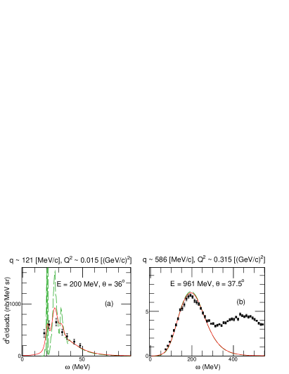
Figure 4: (Color online) Comparison of ¹²C$(e,e^{\prime})$ cross sections obtained with (full line) and without (dashed lines) the folding method. The experimental data are from (a) edata12C:Barreau and (b) edata12C:Sealock .

A limitation of the RPA formalism is that the configuration space is restricted to 1p-1h excitations. As a result only the escape-width contribution to the final-state interaction is accounted for and the spreading width of the particle states is neglected. This affects the description of giant resonances in the CRPA formalism. The energy location of the giant resonance is generally well predicted but the width is underestimated and the height of the response in the peak is overestimated. In order to remedy this, several methods have been proposed such as the folding procedure of Refs. Smith:1988 ; DePace:1993 ; Co:2005 ; Amaro:2007 . Here, we use a simplified phenomenological approach where the modified response functions $R^{\prime}(q,\omega^{\prime})$ are obtained after folding the HF and CRPA response functions $R(q,\omega)$:

$$R^{\prime}(q,\omega^{\prime})=\int_{-\infty}^{\infty}d\omega~{}R(q,\omega)~{}L(\omega,\omega^{\prime}),$$ (23)

with ($L$) a Lorentzian

$$L(\omega,\omega^{\prime})=\frac{1}{2\pi}\left[\frac{\Gamma}{(\omega-\omega^{\prime})^{2}+(\Gamma/2)^{2}}\right].$$ (24)

We use an effective value of $\Gamma$ = 3 MeV which complies well with the predicted energy width in the giant-resonance region [48], where one expects the effect of the folding to be most important. The overall effect of folding is a redistribution of strength from peak to the tails. In line with the conclusions drawn in Refs. Nieves:1997 ; Co:2005 , the energy integrated response functions are not much affected by the folding procedure of Eq. (23). In Fig. 4, we compare the ($e,e^{\prime}$) cross sections obtained with and without folding. Figure 4 (a) clearly shows that in the giant-resonance region, the adopted folding procedure spreads the strength over a wider $\omega$ range, thereby considerably improving the quality of agreement with the data. At higher $\omega$ (Fig. 4 (b)) the effect of the folding is marginal. All computed cross-section results shown in the paper adopt the folding procedure of Eq. (23).

$d^{2}\sigma/d\omega d\Omega$ (nb/MeV sr)

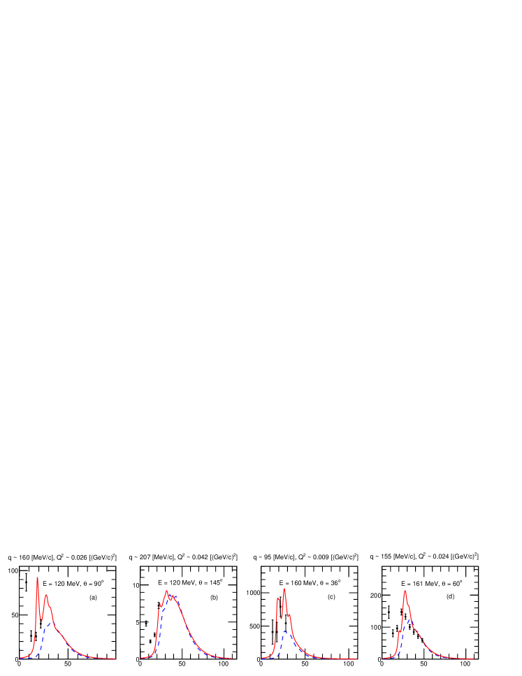
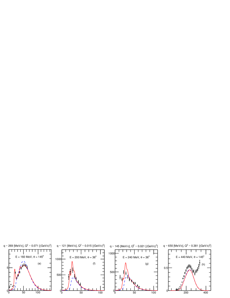
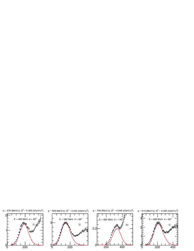
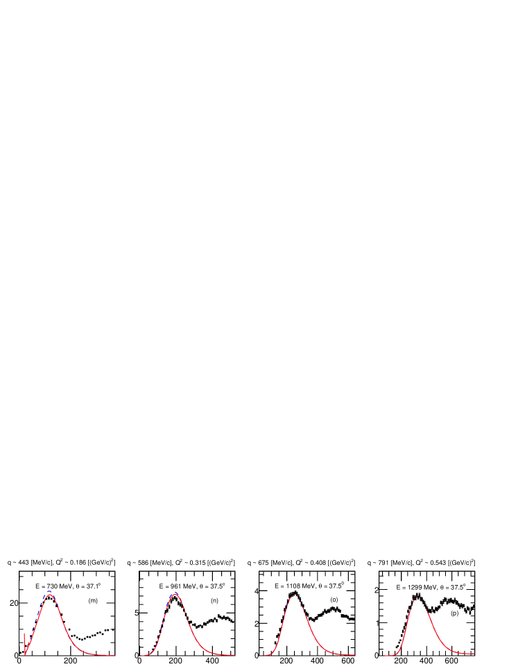
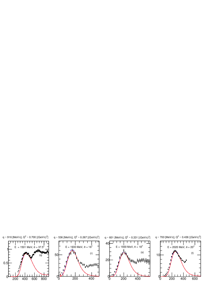
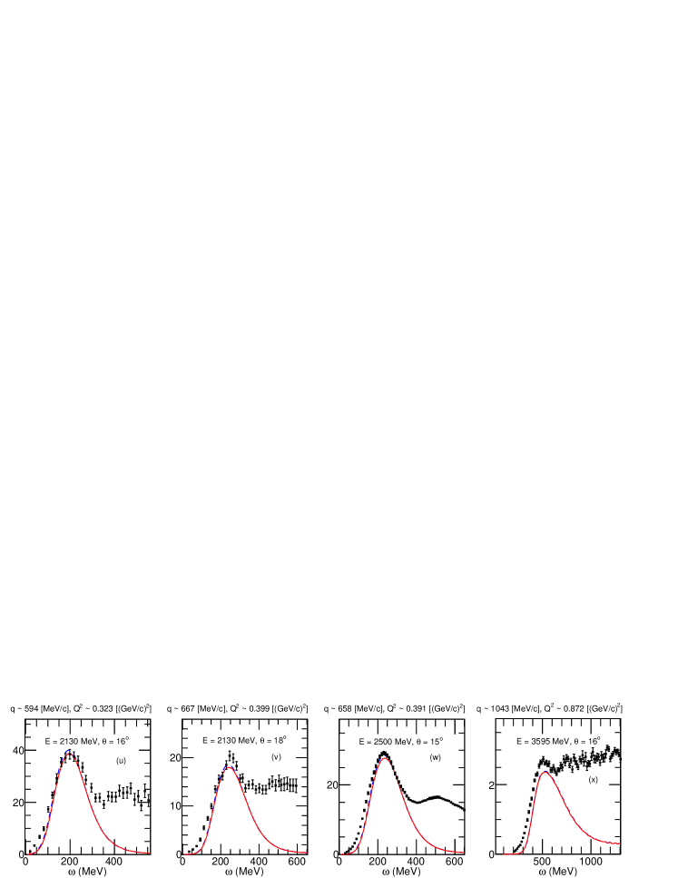
Figure 5: (Color online) The double differential cross section for ¹²C($e,e^{\prime}$). CRPA (solid lines) and HF (dashed-lines) cross sections are compared with the data of Refs. edata12C:Barreau ; edata12C16O:O'Connell ; edata12C:Sealock ; edata12C:Bagdasaryan ; edata12C:Day ; edata12C:Zeller . The $q$ and $Q^{2}$ values, on top of each panel, are calculated at quasielastic conditions $Q^{2}/(2M_{N}\omega)=1$, with $M_{N}$ the nucleon mass.

Our approach is self-consistent because we use the same SkE2 interaction in both the HF and CRPA equations. The parameters of the momentum-dependent SkE2 force are optimized against ground-state and low-excitation energy properties skyrme:physrep1987 . Under those conditions the virtuality $Q^{2}$ of the nucleon-nucleon vertices is small. At high virtualities $Q^{2}$, the SkE2 force tends to be unrealistically strong. We remedy this by introducing a dipole hadronic form factor at the nucleon-nucleon interaction vertices

$$V(Q^{2})~{}\rightarrow V(Q^{2}=0)~{}\frac{1}{(1+\frac{Q^{2}}{\Lambda^{2}})^{2}}$$ (25)

where we introduced the free cut-off parameter $\Lambda$. We adopt $\Lambda~{}=$ 455 MeV, a value which is optimized in a $\chi^{2}$ test of the comparison of $A(e,e^{\prime})$ CRPA cross sections with the experimental data of Refs. edata12C:Barreau ; edata12C16O:O'Connell ; edata12C:Sealock ; edata12C:Bagdasaryan ; edata12C:Day ; edata12C:Zeller ; edata16O:Anghinolfi ; edata40Ca:Williamson . In the $\chi^{2}$ test, we consider the theory-experiment comparison from low values of omega up to the maximum of the quasielastic peak. We have restricted our fit to the low-$\omega$ side of the quasielastic peak, because the high-$\omega$ side is subject to corrections stemming from intermediate $\Delta$ excitation, which is not included in our model.

The influence of the nuclear Coulomb field on the lepton is taken into account by means of an effective momentum approximation (EMA) Engel:1998 . In order to take into account the reduced lepton wavelength, the three-momentum transfer is enhanced in an effective way

$$q_{eff}~{}=~{}q+1.5~{}\left(\frac{Z^{\prime}\alpha\hbar c}{R}\right),$$ (26)

where $R=1.24~{}A^{1/3}$ fm. The lepton wave functions are modified accordingly

$$\Psi_{l}^{eff}~{}=~{}\zeta(Z^{\prime},E,q)~{}\Psi_{l}$$ (27)

with

$$\zeta(Z^{\prime},E,q)~{}=~{}\sqrt{\frac{q_{eff}E_{eff}}{qE}},$$ (28)

where $E$ ($E_{eff}$) is the energy (effective energy) of the outgoing lepton.

Our description of the nuclear dynamics is based on a nonrelativistic framework. For $q>$ 500 MeV/c, the momentum of the emitted nucleon is comparable with its rest mass, and relativistic effects become important. We have implemented relativistic corrections in an effective fashion, as suggested in Refs. Donnelly:1998 ; Amaro:2005 ; Amaro:2007 . Those references show that a satisfactory description of relativistic effects can be achieved by following kinematic substitution in the nuclear response

$$\lambda~{}\rightarrow~{}\lambda\left(1+\lambda\right),$$ (29)

where $\lambda=\omega/2M_{N}$ and $M_{N}$ is the nucleon mass. The above substitution produces a reduction of the width of the one-body responses and a shift in the peak towards smaller values of $\omega$. The correction becomes sizable for $q$ $\gtrsim$ 500 MeV/c.

III Results

To test our model, we start with the calculation of ($e,e^{\prime}$) cross sections on different nuclei and the response functions for electron scattering off ¹²C, in subsection III.1. We confront our numerical results with the data of Refs. edata12C:Barreau ; edata12C16O:O'Connell ; edata12C:Sealock ; edata12C:Bagdasaryan ; edata12C:Day ; edata12C:Zeller ; edata16O:Anghinolfi ; edata40Ca:Williamson ; edataRLRT12C:Jourdan . We discuss the neutrino-scattering results in subsection III.2.

III.1 Electron scattering

In this subsection, we present our results for the QE $A(e,e^{\prime})$ cross sections. For any given $E_{i}$, the nuclear response depends on $q^{\mu}$. Energy transfers below the particle knockout threshold result in nuclear excitations in discrete states. At slightly higher energies, the giant dipole resonance (GDR) shows up. Only at substantially higher energy one can distinguish the peak corresponding to QE one-nucleon knockout. In an ideal case, if an electron scatters from a free nucleon, one would expect a narrow peak at $\omega=Q^{2}/2M_{N}$. Deviations from that peak are due to the nuclear dynamics. The heavier the target nucleus, the wider the peak. The shift of the peak is due to nuclear binding and correlations.

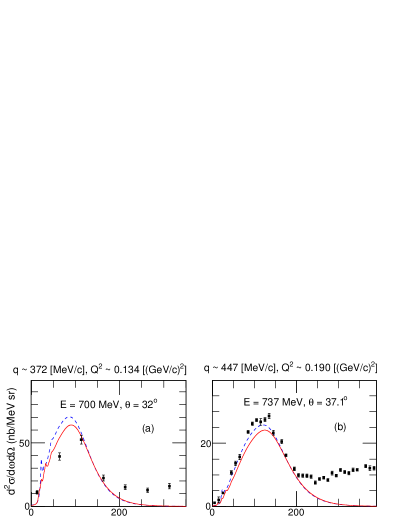
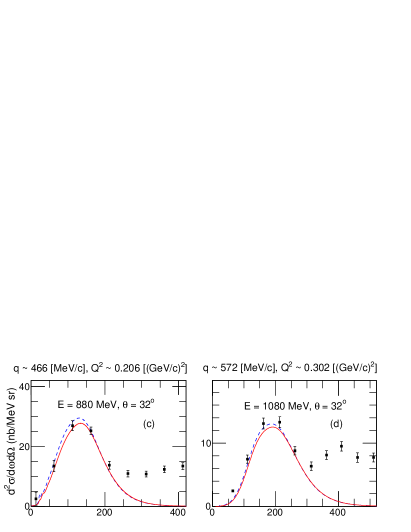
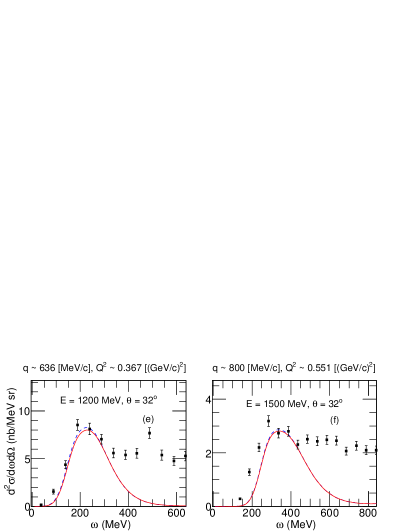
Figure 6: (Color online) As in Fig. 5 but for ¹⁶O($e,e^{\prime}$). The data are from Refs. edata16O:Anghinolfi ; edata12C16O:O'Connell .

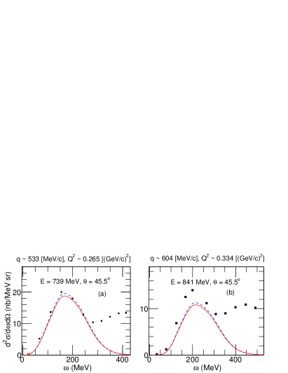
Figure 7: (Color online) Same as Figs. 5 and 6 but on a ⁴⁰Ca target, the measurements are from Ref. edata40Ca:Williamson .

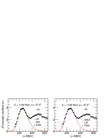
Figure 8: (Color online) Comparison of cross sections obtained (on ¹²C) (a) with the HF and WS single-particle wave functions with SKE2 as residual interaction and (b) with the SKE2 and LM residual interaction with HF as single-particle wave functions.

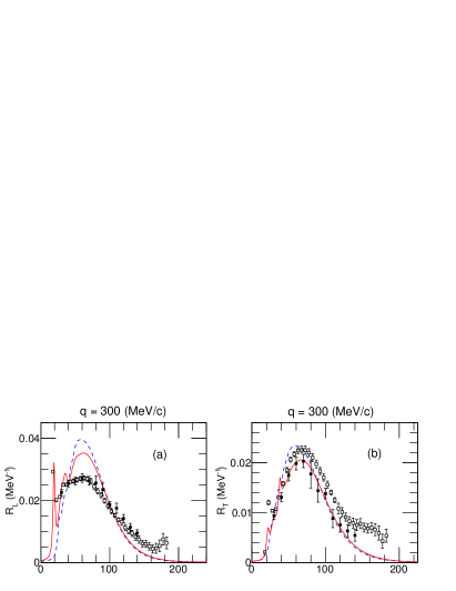
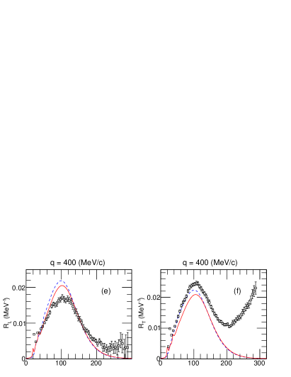
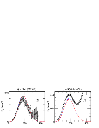
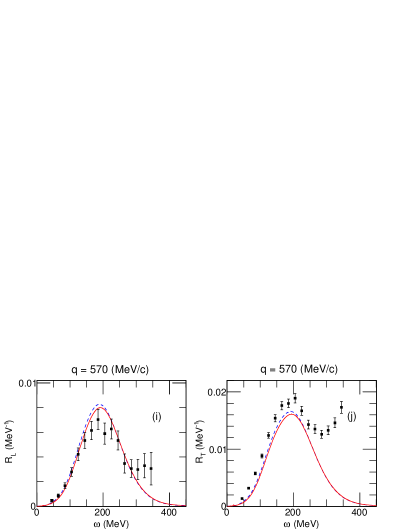
Figure 9: (Color online) Longitudinal and transverse responses for ¹²C($e,e^{\prime}$), for different values of $q$. Solid lines are CRPA predictions and dashed lines are HF predictions. Experimental data are from Ref. edataRLRT12C:Jourdan (filled squares) and Ref. edata12C:Barreau (open squares).

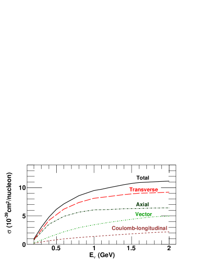
Figure 10: (Color online) Different contributions to the total ¹²C($\nu_{\mu},\mu^{-}$) cross section (per neutron) as a function of incoming neutrino energy. The sum of transverse and Coulomb-longitudinal (axial and vector) is the total cross section.

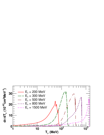
Figure 11: (Color online) Cross section for ¹²C($\nu_{\mu},\mu^{-}$) as a function of outgoing muon kinetic energy $T_{\mu}$, for different incoming neutrino energies. Note the log scale on the horizontal axis.

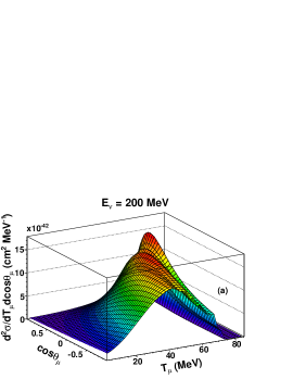
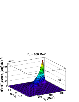
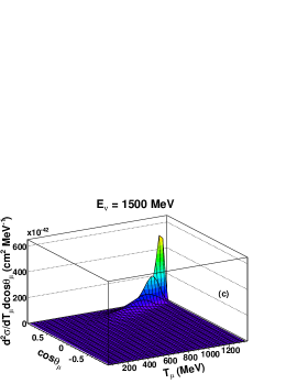
Figure 12: (Color online) Double differential ¹²C($\nu_{\mu},\mu^{-}$) cross sections plotted as a function of $T_{\mu}$ and $\cos\theta_{\mu}$, for three neutrino energies.

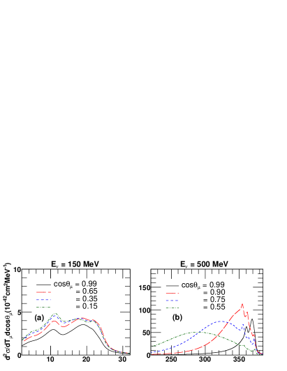
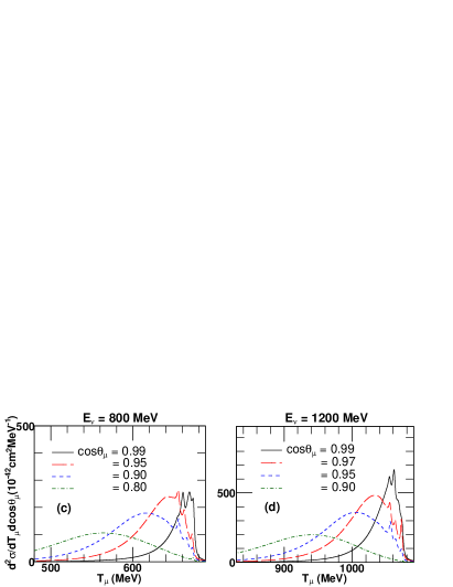
Figure 13: (Color online) Low-energy excitations in double differential cross sections for ¹²C($\nu_{\mu},\mu^{-}$) plotted as a function of $T_{\mu}$, for different $\cos\theta_{\mu}$ values.

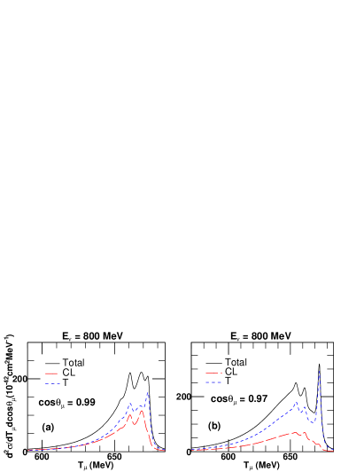
Figure 14: (Color online) Coulomb-longitudinal (CL) and transverse (T) contributions to the double differential cross sections, at $E_{\nu}=$ 800 MeV and two values of $\cos\theta_{\mu}$.

For the two vector form factors entering in the responses, we use the standard dipole parametrization of Ref. dipoleformfactor:1991 . In Fig. 5 we present results of our numerical calculations for ¹²C($e,e^{\prime}$). We compare CRPA and HF predictions with the measurements performed at the Saclay Linear Accelerator edata12C:Barreau , Bates Linear Accelerator Center edata12C16O:O'Connell , Stanford Linear Accelerator Center edata12C:Sealock ; edata12C:Day , Yerevan electron synchrotron edata12C:Bagdasaryan , and DESY edata12C:Zeller . The comparison is performed over a broad range of three- and four-momentum transfers: 95 $\lesssim q\lesssim$ 1050 MeV/c, and 0.009 $\lesssim Q^{2}\lesssim$ 0.900 (GeV/c)². Our predictions are reasonably successful in describing the data over the broad kinematical range considered here. Moreover, they compare favorably with the cross-section results of Refs. Butkevich:2005 ; Ankowski:2014 . The interesting feature of our results is the prediction of the nuclear excitations at small energy ($\omega<$ 50 MeV) and momentum transfers ($q<$ 300 MeV/c), well below the QE peak. This feature can be appreciated in Figs. 5 (a)-5 (g). The HF and CRPA A($e,e^{\prime}$) cross sections are identical for $Q^{2}\gtrsim 0.25$ (GeV/c)². The cross section drops by two orders of magnitude with the shift in scattering angle from $36^{\circ}$ to $145^{\circ}$, for a fixed energy, as evident from Figs. 5 (c)-5(e) for an incoming energy of 160 MeV. Even for higher incoming electron energies the cross-section measurements at smaller scattering angles are still dominated by QE processes. Obviously, the measured cross sections include contributions from channels beyond QE, like $\Delta$-excitations, evident as the second peak in the data, and 2p-2h contributions. Our description is restricted to QE processes and further work is in progress on the role of processes beyond QE ones tom .

The double differential ¹⁶O($e,e^{\prime}$) cross sections are shown in Fig. 6. Our numerical calculations reasonably describe the QE parts of the measurements performed at ADONE edata16O:Anghinolfi and at the Bates Linear Accelerator Center edata12C16O:O'Connell . Further, the calculations for the heavier target ⁴⁰Ca are presented in Fig. 7. Again, the comparison with the experimental data taken at Bates Linear Accelerator Center edata40Ca:Williamson is fair.

In Fig. 8 we compare cross sections obtained with two different parametrizations of the single-nucleon wave functions and nucleon-nucleon residual interactions. The Landau Migdal (LM) Co:1985 and SKE2 Jan:1989 ; skyrme:physrep1987 yield similar cross sections while the use of the Woods-Saxon (WS) Co:1984 wave function slightly shifts and reduces the strength of the cross section. This can be attributed to the fact that the HF wave functions have larger high-momentum components than the WS ones.

The ($e,e^{\prime}$) cross section receives contributions from the longitudinal and transverse components, as can be seen in Eq. (3). A separation of these two response functions provides further detail about the target dynamics. It is worth mentioning that the experimental values of responses are extracted from a set of cross-section measurements using a Rosenbluth separation RLRT:Rosenbluth1950 . The data of Ref. edataRLRT12C:Jourdan is determined by a reanalysis of the world data on ($e,e^{\prime}$) cross sections. Interestingly, that resulted in a significant difference from the measurements of Ref. edata12C:Barreau , as can be seen in Fig. 9 (b). The comparison between our predictions on ¹²C with the experimental data of Refs. edata12C:Barreau ; edataRLRT12C:Jourdan is quite satisfactory. The longitudinal responses are overestimated and the transverse responses are usually underestimated. Our predictions are in line with those predicted in Ref. edataRLRT12C:Jourdan and with the continuum shell model predictions of Ref. Amaro:1999 . It is long known, that the inclusion of processes involving meson exchange current (MEC) are needed to account for the transverse strength of the electromagnetic response Donnelly:1978 ; Alberico:1984 . The calculations carried out on light nuclei overwhelmingly suggest that single-nucleon knockout processes, such as in this work, are dominant in the longitudinal channel while in the transverse channel two-nucleon processes provide substantial contributions.

III.2 Neutrino scattering

The calculation of ¹²C($\nu_{l},l^{-}$) response functions involve two vector form factors and one axial form factor. We use the BBBA05 parametrization of Ref. BBBA05formfactor:2006 for the two vector form factors, and the standard dipole parametrization of the axial form factor with $M_{A}=$ 1.03 $\pm$ 0.02 GeV Beringer:betadecay2012 ; Amsler:2008 ; Bernard:MaWorldAve2002 .

In Fig. 10 we display different contributions to the total ¹²C($\nu_{\mu},\mu^{-}$) cross section, as a function of the incoming neutrino energy. The axial contribution is larger than the vector one. Related to this, neutrino cross sections are dominated by the transverse current.

Electron-scattering cross-section measurements are typically performed for a fixed incoming electron energy and scattering angle. As neutrinos are produced as the secondary products of a decaying primary beam, the interacting neutrino’s energy is not sharply defined. The initial neutrino energy is reconstructed using the kinematics of the final outgoing lepton. This is a major source of uncertainty whereby nuclear structure can have an important influence.

The neutrino flux in oscillation experiments typically covers a wide energy range from about 100 MeV to a few GeV. The cross section measured at a single energy and scattering angle of the outgoing lepton picks up contributions from scattering processes at different energies, with varying weights. In Fig. 11, we show the differential cross section (in outgoing muon energy) for 200 $\lesssim E_{\nu}\lesssim$ 1500 MeV. It is evident from the figure that with increasing $E_{\nu}$ the strengths of the cross sections shift in muon energy. Also, there is a clear signature of the low-$\omega$ excitations even at neutrino energies around the peak of the MiniBooNE and T2K $\nu_{\mu}$ spectra.

The measured cross sections are flux-folded double differential in outgoing muon kinetic energy $T_{\mu}$ and scattering angle $\cos\theta_{\mu}$. To illustrate the low-energy excitations and general behavior of double differential ¹²C$(\nu_{\mu},\mu^{-})$ cross sections at fixed energies, we display in Fig. 12 the double differential cross sections for $E_{\nu}=$ 200, 800, and 1500 MeV. With the increase in incoming neutrino energy, the strength shifts in the forward direction and the width of giant resonances reduces. In Fig. 13, we plot the double differential cross section at different fixed values of $\cos\theta_{\mu}$. For $E_{\nu}=$ 150 MeV, the double differential cross section is dominated by low-lying nuclear excitations, as evident from Fig. 13 (a). For neutrino energies around the mean energy of the MiniBooNE miniboone:ccqenu and T2K t2k:qenu fluxes, $E_{\nu}=$ 800 MeV [Fig. 13 (c)], the nuclear collective excitations are still sizable at forward muon scattering angles. The same feature is still visible for very forward scattering off neutrinos with an energy of 1200 MeV [Fig. 13(d)]. The contribution of collective excitations to neutrino-nucleus responses can not be accounted for within the RFG-based simulation codes. As evident from the results presented here, they can account for non-negligible contributions to the signal even at higher neutrino energies.

In Fig. 14, we show the transverse and Coulomb-longitudinal contribution to the double differential cross sections. For $\cos\theta_{\mu}=$ 0.99, the Coulomb-longitudinal contribution of the quasielastic cross section is comparable to the transverse one. The transverse contribution dominates the cross section as soon as one moves away from the very forward direction. This feature along with the giant-resonance contribution to forward-scattering cross sections accounts for most of the strength at very small momentum transfers. Theoretical models, which do not predict this behavior, tend to underestimate the cross section for forward-scattering angles, as discussed in Ref. Martini:2014 .

IV Conclusions

We presented a detailed discussion of CRPA predictions for quasielastic electron-nucleus and neutrino-nucleus responses.

We assessed inclusive quasielastic electron-nucleus cross sections on ¹²C, ¹⁶O, and ⁴⁰Ca. We consider momentum transfers over the broad range 95 $\lesssim q\lesssim$ 1050 MeV/c in combination with energy transfers which favor the quasielastic nucleon-knockout reaction process. We confronted our predictions with high-precision electron-scattering data. We separated the longitudinal and transverse responses on ¹²C, for 300 $\lesssim q\lesssim$ 570 MeV/c, and compared them with the data. A reasonable overall description of the data, especially those corresponding with low-energy nuclear excitations, is reached.

We calculated ¹²C($\nu_{\mu},\mu^{-}$) cross sections, relevant for accelerator-based neutrino-oscillation experiments. We illustrated how low-energy nuclear excitations are induced by neutrinos. We paid special attention to contributions where nuclear-structure details become important, but remain unobserved in RFG-based models. We show that low-energy excitations can account for non-negligible contributions to the signal of accelerator-based neutrino-oscillation experiments, especially at forward neutrino-nucleus scattering.

- (1) A. A. Aguilar-Arevalo et al., (MiniBooNE Collaboration), Phys. Rev. D81, 092005 (2010).
- (2) A. A. Aguilar-Arevalo et al., (MiniBooNE Collaboration), Phys. Rev. D88, 032001 (2013).
- (3) A. A. Aguilar-Arevalo et al., (MiniBooNE Collaboration), Phys. Rev. D82, 092005 (2010).
- (4) G. A. Fiorentini et al., (MINERvA Collaboration), Phys. Rev. Lett. 111, 022502 (2013).
- (5) L. Fields et al., (MINERvA Collaboration), Phys. Rev. Lett. 111, 022501 (2013).
- (6) K. Abe et al., (T2K Collaboration), Phys. Rev. D87, 092003 (2013).
- (7) K. Abe et al., (T2K Collaboration), arXiv:1407.4256[hep-ex].
- (8) J. G. Morfin, J. Nieves, and J. T. Sobczyk, Adv. High Energy Phys. 2012, 934597 (2012).
- (9) L. Alvarez-Ruso, Y. Hayato, J. Nieves, New J. Phys. 16, 075015 (2014).
- (10) E. Kolbe, K. Langanke, F. K. Thielemann, and P. Vogel, Phys. Rev. C 52, 3437 (1995).
- (11) C. Volpe, N. Auerbach, G. Colo, T. Suzuki, and N. Van Giai, Phys. Rev. C 62, 015501 (2000).
- (12) A. Botrugno, and G. Co’, Nucl. Phys. A761, 200 (2005).
- (13) M. Martini, G. Co’, M. Anguiano, and A. M. Lallena, Phys. Rev. C 75, 034604 (2007).
- (14) A. R. Samana, F. Krmpotic, N. Paar, C. A. Bertulani, Phys. Rev. C 83, 024303 (2011).
- (15) http://www-boone.fnal.gov/
- (16) http://t2k-experiment.org/
- (17) W. M. Alberico, M. Ericson, and A. Molinari, Nucl. Phys. A 379, 429 (1982).
- (18) M. Martini, M. Ericson, G. Chanfray, and J. Marteau, Phys. Rev. C 80, 065501 (2009).
- (19) M. Martini J. Phys. Conf. Ser. 408, 012041 (2013).
- (20) A. Gil, J. Nieves, and E. Oset, Nucl. Phys. A 627, 543 (1997).
- (21) J. Nieves, J. E. Amaro, and M. Valverde, Phys. Rev. C 70, 055503 (2004).
- (22) J. Nieves, M. Valverde, and M. J. Vicente Vacas, Phys. Rev. C 73, 025504 (2006).
- (23) O. Benhar, A. Fabrocini, S. Fantoni, and I. Sick, Nucl. Phys. A 579, 493 (1994).
- (24) O. Benhar, N. Farina, H. Nakamura, M. Sakuda, and R. Seki, Phys. Rev. D 72, 053005 (2005).
- (25) H. Nakamura, T. Nasu, M. Sakuda, and O. Benhar, Phys. Rev. C 76, 065208 (2007).
- (26) A. M. Ankowski, O. Benhar, and M. Sakuda, Phys. Rev. D 91, 033005 (2015).
- (27) J. E. Amaro, M. B. Barbaro, J. A. Caballero, T. W. Donnelly, and C. Maieron, Phys. Rev. C71, 065501 (2005).
- (28) J. E. Amaro, M. B. Barbaro, J. A. Caballero, T. W. Donnelly, and J. M. Udias, Phys. Rev. C75, 034613 (2007).
- (29) T. Leitner, O. Buss, L. Alvarez-Ruso, and U. Mosel, Phys. Rev. C 79, 034601 (2009).
- (30) A. V. Butkevich, and S. P. Mikheyev, Phys. Rev. C 72, 025501 (2005).
- (31) A. V. Butkevich, and S. A. Kulagin, Phys. Rev. C 76, 045502 (2007).
- (32) A. Meucci, F. Capuzzi, C. Giusti, and F. D. Pacati, Phys. Rev. C 67, 054601 (2003).
- (33) A. Meucci, C. Giusti, and F. D. Pacati, Nucl. Phys. A 739, 277 (2004).
- (34) G. Co’, and S. Krewald, Phys. Lett. B137, 145 (1984).
- (35) S. Jeschonnek, T. W. Donnelly, Phys. Rev. C57, 2438 (1998).
- (36) J. Ryckebusch, M. Waroquier, K. Heyde, J. Moreau, and D. Ryckbosch, Nucl. Phys. A476, 237 (1988).
- (37) J. Ryckebusch, K. Heyde, D. Van Neck, and M. Waroquier, Nucl. Phys. A503, 694 (1989).
- (38) N. Jachowicz, S. Rombouts, K. Heyde, and J. Ryckebusch, Phys. Rev. C59, 3246 (1999).
- (39) N. Jachowicz, K. Heyde, J. Ryckebusch, and S. Rombouts, Phys. Rev. C65, 025501 (2002).
- (40) N. Jachowicz, K. Vantournhout, J. Ryckebusch, and K. Heyde, Phys. Rev. Lett. 93, 082501 (2004).
- (41) N. Jachowicz, G. C. McLaughlin, Phys. Rev. Lett. 96, 172301 (2006).
- (42) N. Jachowicz, C. Praet, and J. Ryckebusch, Acta Physica Polonica B 40, 2559 (2009).
- (43) N. Jachowicz, and V. Pandey, AIP Conf. Proc. 1663, 050003 (2015).
- (44) V. Pandey, N. Jachowicz, J. Ryckebusch, T. Van Cuyck, and W. Cosyn, Phys. Rev. C89, 024601 (2014).
- (45) J. Engel, Phys. Rev. C57, 2004 (1998).
- (46) J. S. O’Connell, T. W. Donnelly, and J. D. Walecka, Phys. Rev. C6, 719 (1972).
- (47) J. D. Walecka, Theoretical Nuclear and Subnuclear Physics (Oxford University Press, New York, 1995).
- (48) R. D. Smith, J. Wambach, Phys. Rev. C38, 100 (1988).
- (49) A. De Pace, and M. Viviani, Phys. Rev. C48, 2931 (1993).
- (50) M. Waroquier, J. Ryckebusch, J. Moreau, K. Heyde, N. Blasi, S. .Y. Van de Werf and G. Wenes, Phys. Rept. 148, 249 (1987).
- (51) P. Barreau et al., Nucl. Phys. A402, 515 (1983).
- (52) J. S. O’Connell et al., Phys. Rev. C35, 1063 (1987).
- (53) R. M. Sealock et al., Phys. Rev. Lett.62, 1350 (1989).
- (54) D. S. Bagdasaryan et al., YERPHI-1077-40-88 (1988).
- (55) D. B. Day et al., Phys. Rev. C 48, 1849 (1993).
- (56) D. Zeller, DESY-F23-73-2 (1973).
- (57) M. Anghinolfi et al., Nucl. Phys. A602, 405 (1996).
- (58) C. F. Williamsonet al., Phys. Rev. C56, 3152 (1997).
- (59) J. Jourdan, Nucl. Phys. A603, 117 (1996).
- (60) E. J. Beise, and R. D. McKeown, Comments Nucl. Part. Phys., 20, 105 (1991).
- (61) T. Van Cuyck, N. Jachowicz, M. Martini, V. Pandey, J. Ryckebusch, in preparation.
- (62) G. Có, and S. Krewald, Nucl. Phys. A 433, 392 (1985).
- (63) M. N. Rosenbluth, Phys. Rev. 79, 615 (1950).
- (64) J. E. Amaro, G. Co’, A. .M. Lallena, arXiv:9902072 [nucl-th].
- (65) T. W. Donnelly, J. W. Van Orden, T. De Forest, Jr., and W. C. Hermans, Phys. Lett. B 76, 393 (1978).
- (66) W. M. Alberico, M. Ericson, and A. Molinari, Ann. Phys. 154, 356 (1984).
- (67) R. Bradford, A. Bodek, H. Budd, and J. Arrington, Nucl. Phys. Proc. Suppl. 159, 127 (2006).
- (68) J. Beringer et al., (Particle Data Group), Phys. Rev. D 86, 010001 (2012).
- (69) C. Amsler et al., (Particle Data Group), Phys. Lett. 667B, 1 (2008).
- (70) V. Bernard, L. Elouadrhiri, and U. G. Meissner, J. Phys. G 28, R1 (2002).
- (71) M. Martini, M. Ericson, Phys. Rev. C 90, 025501 (2014).