Electromagnetic matrix elements for negative parity nucleons

Abstract:

Here we present preliminary results for the evaluation of the electromagnetic form factors for the lowest-lying negative-parity, spin-$\nicefrac{{1}}{{2}}$ nucleons, namely the $S_{11}(1535)$ and $S_{11}(1650)$, through the use of the variational method. We find that the characteristics of the electric form factor, $G_{E}$, are similar between these states, however significant differences are observed between the quark-sector contributions to the magnetic form factor, $G_{M}$. Within simple constituent quark models, these states are understood to be admixtures of $s=\nicefrac{{1}}{{2}}$ and $s=\nicefrac{{3}}{{2}}$ states coupled to orbital angular momentum $\ell=1$. Our results reveal a qualitative difference in the manner in which the singly-represented quark sector contributes to these baryon magnetic form factors.

1 Introduction

Over the past decade there has been significant experimental interest in mapping out the excited nucleon spectrum and understanding the underlying dynamics and structure of these states. Such data provides an excellent opportunity to connect experiment with theoretical expectations to gain further insight into hadronic excitations. The success of using variational techniques to explore the hadron spectrum from Lattice QCD has shown that these methods can be utilised for calculations of both ground state [1] and excited state [2, 3] matrix elements. In this work we perform an evaluation of the electromagnetic form factors of the lowest-lying spin-$\nicefrac{{1}}{{2}}$ negative-parity nucleon states.

2 Accessing negative parity states

The simplest approach to evaluating the correlators relevant to accessing negative-parity nucleons [4] is to use the standard nucleon interpolator coupled with an additional $\gamma_{5}$ matrix in order to change its parity transformation properties, $\chi_{p}(x)\rightarrow\chi^{-}_{p}(x)=\gamma_{5}\chi_{p}(x)$. One then evaluates the two-point correlator in the standard fashion and projects out the state via the standard projection operator $\Gamma=\left(\frac{\gamma_{0}+I}{2}\right)$

$$G_{-}(\vec{p},t;\Gamma) =\sum_{\vec{x}}e^{-i\vec{p}\cdot\vec{x}}\mathrm{tr}\left[\Gamma\,\langle\,\Omega\,|\,\chi^{-}_{p}(x)\,\overline{\chi}^{-}_{p}(0)\,|\,\Omega\rangle\right]$$ (1)

$$=-\sum_{\vec{x}}e^{-i\vec{p}\cdot\vec{x}}\mathrm{tr}\left[\Gamma\,\langle\,\Omega\,|\,\gamma_{5}\chi_{p}(x)\,\overline{\chi}_{p}(0)\gamma_{5}\,|\,\Omega\rangle\right]\,.$$ (2)

However using the cyclicity of the trace, one could instead access the relevant contributions for negative parity states from the correlator evaluated with the positive parity operator if one instead uses the modified projector

$$\Gamma^{-}=-\gamma_{5}\Gamma\gamma_{5}=\left(\frac{\gamma_{0}-I}{2}\right)\,.$$ (3)

Such an approach has long been established as the optimal method for studying negative parity states. However, we outline this in detail here as the arguments carry over naturally to the evaluation of three-point correlation functions. Again, one could evaluate the three-point correlator for a negative parity nucleon through

$$G^{\mu}_{-}(\vec{p}\>\!^{\prime},\vec{p};t_{2},t_{1};\Gamma^{\prime}) =\;\;\;\;\sum_{\vec{x}_{2},\vec{x}_{1}}e^{-i\vec{p}\>\!^{\prime}\cdot\vec{x}_{2}}e^{+i(\vec{p}\>\!^{\prime}-\vec{p})\cdot\vec{x}_{1}}\mathrm{tr}\left[\Gamma^{\prime}\,\langle\,\Omega\,|\,\chi^{-}_{p}(x_{2})j^{\mu}(x_{1})\overline{\chi}^{-}_{p}(0)\,|\,\Omega\,\rangle\right]$$ (4)

$$=-\sum_{\vec{x}_{2},\vec{x}_{1}}e^{-i\vec{p}\>\!^{\prime}\cdot\vec{x}_{2}}e^{+i(\vec{p}\>\!^{\prime}-\vec{p})\cdot\vec{x}_{1}}\mathrm{tr}\left[\Gamma^{\prime}\,\langle\,\Omega\,|\,\gamma_{5}\chi_{p}(x_{2})j^{\mu}(x_{1})\overline{\chi}_{p}(0)\gamma_{5}\,|\,\Omega\,\rangle\right]\,.$$ (5)

However, we can again access the necessary terms by evaluating correlators with the positive parity operators and projecting with the modified projector, $\left(\Gamma^{\prime}\right)^{-}=-\gamma_{5}\Gamma^{\prime}\gamma_{5}$.

3 Variational Methods for matrix element determination

The goal of the this approach is to produce a set of operators $\phi^{\alpha}$ that satisfy

$$\langle\Omega|\phi^{\alpha}|\beta,p,s\rangle=\delta^{\alpha\beta}\,.$$ (6)

This is realised by taking an existing basis of operators $\{\chi_{i}\}$ and constructing the desired operators as linear superpositions

$$\phi^{\alpha}(x)=\sum_{i}v^{\alpha}_{i}\,\chi_{i}(x)\>,\hskip 20.0pt\overline{\phi}\,{}^{\alpha}(x)=\sum_{j}\overline{\chi}_{j}(x)\,u^{\alpha}_{j}\,.$$ (7)

Starting from the matrix of cross correlators

$$G_{ij}(\vec{p},t;\,\Gamma)=\sum_{\vec{x}}e^{-i\vec{p}\cdot\vec{x}}\mathrm{tr}\left[\Gamma\langle\Omega|\chi_{i}(x)\overline{\chi}_{j}(0)|\Omega\rangle\right]\,,$$ (8)

and noting $G_{ij}(\vec{p},t;\Gamma)\,u^{\alpha}_{j}$ provides a recurrence relation with time dependence $e^{-E_{\alpha}t}$, one can show that the necessary vectors $v^{\alpha}_{i}$ and $u^{\alpha}_{j}$ are the eigenvectors of the generalised eigenvalue equations

$$v^{\alpha}_{i}\>G_{ij}(\vec{p},t_{0}+\Delta t;\,\Gamma)\hskip 13.0pt =e^{-E_{\alpha}\Delta t}\>v^{\alpha}_{i}\>G_{ij}(\vec{p},t_{0};\,\Gamma)\,,$$ (9a)

$$\hskip 13.0ptG_{ij}(\vec{p},t_{0}+\Delta t;\,\Gamma)\>u^{\alpha}_{j} =e^{-E_{\alpha}\Delta t}\>\hskip 13.0ptG_{ij}(\vec{p},t_{0};\,\Gamma)\>u^{\alpha}_{j}\,.$$ (9b)

It is worth noting that these equations are evaluated for a given 3-momentum $\vec{p}$ and projection operator $\Gamma$ and so the corresponding operators satisfy Eq. (6) for this momentum and parity only. One can obtain the correlator for the state $\alpha$ by projecting with the corresponding eigenvectors

$$G^{\alpha}(\vec{p},t;\Gamma)\equiv v^{\alpha}_{i}(\vec{p})\>G_{ij}(\vec{p},t;\Gamma)\>u^{\alpha}_{j}(\vec{p})\,,$$ (10)

from which the desired quantities are extracted in the standard way. To access the corresponding three-point correlator, it is a simple matter of applying the relevant eigenvectors to the corresponding three-point function, where care is taken to ensure that the projection is done with the correct momenta for source and sink

$$G^{\alpha}(\vec{p}\>\!^{\prime},\vec{p},t_{2},t_{1};\,\Gamma^{\prime})\equiv v^{\alpha}_{i}(\vec{p}\>\!^{\prime})\>G_{ij}(\vec{p}\>\!^{\prime},\vec{p},t_{2},t_{1};\,\Gamma^{\prime})\>u^{\alpha}_{j}(\vec{p})\,.$$ (11)

From the projected two and three-point functions one then continues on in the standard way by constructing a suitable ratio to isolate the desired matrix element. Here we choose to use the ratio as defined in Ref. [5]. Using the modified projectors outlined in the previous section, we arrive at the ratio used in the determination of the form factors

$$R^{\alpha}_{-}(\vec{p}\>\!^{\prime},\vec{p};\Gamma^{\prime},\Gamma)=\sqrt{\frac{\langle G^{\alpha}(\vec{p}\>\!^{\prime},\vec{p},t_{2},t_{1};\left(\Gamma^{\prime}\right)^{-})\rangle\,\langle G^{\alpha}(\vec{p},\vec{p}\>\!^{\prime},t_{2},t_{1};\left(\Gamma^{\prime}\right)^{-})\rangle}{\langle G^{\alpha}(\vec{p}\>\!^{\prime},t_{2};\Gamma^{-})\rangle\,\langle G^{\alpha}(\vec{p},t_{2};\Gamma^{-})\rangle}}\,.$$ (12)

4 Negative Parity Baryon Form Factors

Here we consider the electromagnetic form factors for a negative parity, spin-$\nicefrac{{1}}{{2}}$ baryon. To make the connection with the familiar positive parity case, we note that negative-parity baryon spinors can be defined relative to positive parity spinors by again multiplying by a $\gamma_{5}$ matrix and attributing the odd-parity baryon mass to considerations of $p$

$$u(p,s)\rightarrow u_{-}(p,s)=\gamma_{5}\,u(p,s)\,.$$ (13)

One can then show through the vertex decomposition presented in Refs. [6, 7] that it is possible to write the $+\rightarrow+$ and $-\rightarrow-$ transitions, of which the elastic processes are a special case, in a common form. With this understanding it follows that the matrix element can be expressed as

$$\langle\,N^{-},p^{\prime},s^{\prime}\,|\,j^{\mu}(0)\,|\,N^{-},p,s\,\rangle=\left(\frac{M^{2}}{E_{p}E_{p^{\prime}}}\right)^{\nicefrac{{1}}{{2}}}u(p^{\prime},s^{\prime})\left(\gamma^{\mu}F_{1}(Q^{2})+i\frac{\sigma^{\mu\nu}q_{\nu}}{2M}F_{2}(Q^{2})\right)u(p,s)\,.$$ (14)

These are in turn related to the Sachs Electric and Magnetic form factors

$$G_{E}(Q^{2}) =F_{1}(Q^{2})-\frac{Q^{2}}{(2M)^{2}}F_{2}(Q^{2})\,,$$ (15)

$$G_{M}(Q^{2}) =F_{1}(Q^{2})+F_{2}(Q^{2})\,.$$ (16)

To isolate these form factors, we follow the approach outlined in Refs. [8, 9]. Having projected out the correlators relevant for the state $|\alpha\rangle$ and formed the necessary ratio, we choose the incoming state to be at rest and so extract $G_{E}$ and $G_{M}$ through the following terms

$$G_{E}(Q^{2})=\overline{R}^{4}_{-}(\vec{q},0;\Gamma_{4},\Gamma_{4})\,,\quad G_{M}(Q^{2})=\frac{(E_{q}+M)}{|\vec{q}|}\overline{R}^{3}_{-}(\vec{q},0;\Gamma_{2},\Gamma_{4})\,,$$ (17)

where $\overline{R}$ is the reduced ratio

$$\overline{R}^{\mu}_{-}(\vec{p}\>\!^{\prime},\vec{p};\Gamma)=\left[\frac{2E_{p}}{E_{p}+M}\right]^{\nicefrac{{1}}{{2}}}\left[\frac{2E_{p^{\prime}}}{E_{p^{\prime}}+M}\right]^{\nicefrac{{1}}{{2}}}R^{\mu}_{-}(\vec{p}\>\!^{\prime},\vec{p};\Gamma)\,.$$ (18)

5 Calculation Details

The states of interest, the $S_{11}(1535)$ and the $S_{11}(1650)$, have been isolated in a previous CSSM study [10] and so we shall use the same operator basis and parameters in our variational analysis. To form our operator basis we use local nucleon operators

$$\chi_{1}(x)=\epsilon^{abc}\left(u^{Ta}(x)\,C\gamma_{5}\,d^{b}(x)\right)u^{c}(x)\,,\quad\chi_{2}(x)=\epsilon^{abc}\left(u^{Ta}(x)\,C\,d^{b}(x)\right)\gamma_{5}u^{c}(x)\,,$$ (19)

coupled with varying levels of gauge-invariant Gaussian smearing applied to both fermion source and sink. In particular, we use 16, 35, 100 and 200 sweeps of smearing applied to the spatial dimensions only, with a smearing fraction $\alpha=0.7$. This allows for the construction of an 8 $\times$ 8 correlation matrix. For the variational parameters we use $t_{0}=18$ and $\Delta t=2$ relative to the quark source at $t=16$. The calculation is performed on the PACS-CS 2 + 1 flavour dynamical gauge-field configurations [11] made available through the ILDG [12]. These configurations use an ${\cal O}(a)$-improved Wilson-Clover fermion action and Iwasaki gauge-action, with $\beta=1.90$ resulting in a lattice spacing $a=0.0907$ fm. The lattices have dimension $32^{3}$ $\times$ $64$ giving rise to a spatial box of length $L=2.9$ fm. We have access to five light quark masses, with the strange quark mass held fixed. The resulting pion masses range from 702 MeV right down to 156 MeV. The resulting spectrum is presented in Fig. 1. We observe two low-lying eigenstates with small mass difference, consistent with the experimentally observed masses for the $S_{11}(1535)$ and $S_{11}(1650)$. It is these states whose form factors we shall examine herein.

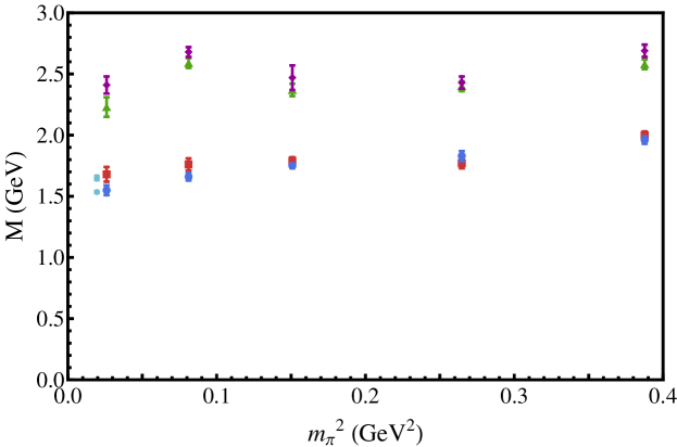
Figure 1: The four lowest lying-states observed in our $\nicefrac{{1}}{{2}}^{-}$ nucleon spectrum obtained via an 8 $\times$ 8 correlation matrix formed from smeared $\chi_{1}$ and $\chi_{2}$ interpolators. The light blue data points correspond to the PDG values [14] for the negative parity nucleon states with 3-star determination or higher.

For the SST inversion we choose to use the fixed current method with a conserved-vector current inserted at $t_{S}=21$. For our error analysis we use a second-order single-elimination jackknife method where the $\chi^{2}_{\textrm{dof}}$ is obtained via a covariance matrix analysis. For the form factors we consider all but the lightest quark mass. The eigenstate projected correlators are fitted to a single state ansatz. By studying the regions where $\log(G)$ behaves linearly we ensure that the correlator is dominated by a single energy eigenstate. Further discussion can be found in Refs. [3, 13].

6 Results

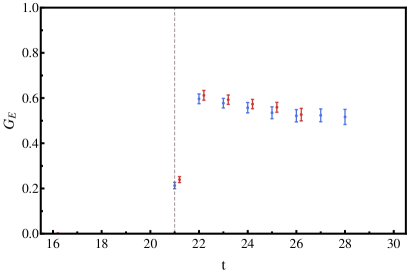
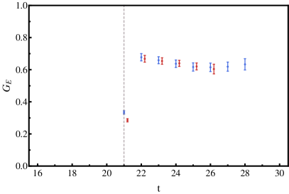
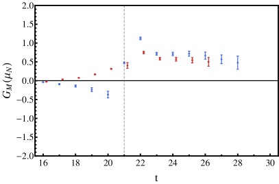
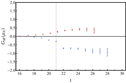
Figure 2: The doubly-represented (left) and singly-represented (right) quark sector contributions to the the Sachs electric form factor $G_{E}$ for $m_{\pi}=0.570$ GeV. Results are provided for single quarks of unit charge. The blue data points correspond to the $S_{11}(1535)$ while the red data points to the $S_{11}(1650)$.

Figure 3: The doubly-represented (left) and singly-represented (right) quark sector contributions to the the Sachs magnetic form factor $G_{M}$ for $m_{\pi}=0.570$ GeV. Results are provided for single quarks of unit charge. Again, the blue data points correspond to the $S_{11}(1535)$ while the red data points to the $S_{11}(1650)$.

In Figs. 2 and 3 we present the quark-sector results for the electric and magnetic form factors respectively. We present results for single quarks of unit charge. The data is presented at a single quark mass corresponding to $m_{\pi}=0.570$ GeV. However, all masses considered display behaviour consistent with that in Fig. 2 and 3. The colours match up with the states presented in Fig. 1, with the blue identified as the $S_{11}(1535)$ and the red as the $S_{11}(1650)$.

We note that due to the similar masses between these two states, we are probing each state at essentially the same value of $Q^{2}$. For the electric form factor, we find that both states take on very similar values in both quark sectors, with the doubly-represented quark-sector form factor slightly smaller than the singly-represented sector. Examining the magnetic quark sector we see distinctly different behaviour between these two states. Though the doubly-represented quark sector is similar, we find that the singly-represented quark sector in the $S_{11}(1650)$ is positive (same sign as the doubly-represented sector) while the corresponding contribution in the $S_{11}(1535)$ is negative. Furthermore, the magnitude of the singly-represented quark contribution is somewhat larger in the $S_{11}(1535)$ than it is in the $S_{11}(1650)$.

7 Conclusions

Herein we have presented the first lattice QCD calculation of the electromagnetic form factors of the two lowest-lying spin-$\nicefrac{{1}}{{2}}$ negative-parity nucleons. Using variational techniques we are able to disentangle the relevant matrix element for these two states, allowing us to probe their underlying structure.

Both states display very similar values in their electric form factor. However, comparison of the magnetic form factor highlights distinctly different behaviour in the quark sector contributions. Such behavior is anticipated in simple quark models due to differences in the underlying space-spin-flavour symmetry construction of these states.

The difference in the sign between the doubly-represented and singly-represented quark contributions in the $S_{11}(1535)$ and the sign symmetry of quark sector contributions in the $S_{11}(1650)$ will give rise to significantly different baryon form factors. It will be interesting to compare these with phenomenological estimates and gain insight into the mechanisms of QCD giving rise to these observations. Future work will generalise these techniques to examine the corresponding helicity amplitudes for these states, central to the radiative transitions measured in experimental programs.

References

[1]
B. J. Owen, J. Dragos, W. Kamleh, D. B. Leinweber, M. S. Mahbub, B. J. Menadue and J. M. Zanotti,
Variational Approach to the Calculation of gA,
Phys. Lett. B 723, 217 (2013)
[arXiv:1212.4668 [hep-lat]].
[2]
B. Owen, W. Kamleh, D. B. Leinweber, S. Mahbub and B. Menadue,
Correlation matrix methods for excited meson form factors in full QCD,
PoS LATTICE 2012, 173 (2012).
[3]
B. J. Owen, W. Kamleh, D. B. Leinweber, M. S. Mahbub and B. J. Menadue,
Probing the proton and its excitations in full QCD,
PoS LATTICE 2013, 277 (2013)
[arXiv:1312.0291 [hep-lat]].
[4]
F. X. Lee and D. B. Leinweber,
Nucl. Phys. Proc. Suppl. 73, 258 (1999)
[hep-lat/9809095].
[5]
J. N. Hedditch, W. Kamleh, B. G. Lasscock, D. B. Leinweber, A. G. Williams and J. M. Zanotti,
Pseudoscalar and vector meson form-factors from lattice QCD,
Phys. Rev. D 75, 094504 (2007)
[hep-lat/0703014 [HEP-LAT]].
[6]
R. C. E. Devenish, T. S. Eisenschitz and J. G. Korner,
Electromagnetic Transition Form-Factors,
Phys. Rev. D 14, 3063 (1976).
[7]
I. G. Aznauryan, V. D. Burkert and T.-S. H. Lee,
On the definitions of the helicity amplitudes,
arXiv:0810.0997 [nucl-th].
[8]
D. B. Leinweber, R. M. Woloshyn and T. Draper,
Electromagnetic structure of octet baryons,
Phys. Rev. D 43, 1659 (1991).
[9]
S. Boinepalli, D. B. Leinweber, A. G. Williams, J. M. Zanotti and
J. B. Zhang,
Precision electromagnetic structure of octet baryons in the
chiral regime,
Phys. Rev. D 74, 093005 (2006)
[hep-lat/0604022].
[10]
M. S. Mahbub et al.,
Low-lying Odd-parity States of the Nucleon in Lattice QCD,
Phys. Rev. D 87, 011501 (2013)
[arXiv:1209.0240 [hep-lat]].
[11]
S. Aoki et al. [PACS-CS Collaboration],
2+1 Flavor Lattice QCD toward the Physical Point,
Phys. Rev. D 79, 034503 (2009)
[arXiv:0807.1661 [hep-lat]].
[12]
M. G. Beckett, B. Joo, C. M. Maynard, D. Pleiter, O. Tatebe and T. Yoshie,
Building the International Lattice Data Grid,
Comput. Phys. Commun. 182, 1208 (2011)
[arXiv:0910.1692 [hep-lat]].
[13]
M. S. Mahbub, W. Kamleh, D. B. Leinweber and A. G. Williams,
Searching for low-lying multi-particle thresholds in lattice spectroscopy,
Annals Phys. 342, 270 (2014)
[arXiv:1310.6803 [hep-lat]].
[14]
K. A. Olive et al. [Particle Data Group Collaboration],
Review of Particle Physics,
Chin. Phys. C 38, 090001 (2014).