Nonlinear optomechanical paddle nanocavities

Abstract

Nonlinear optomechanical coupling is the basis for many potential future experiments in quantum optomechanics (e.g., quantum non-demolition measurements, preparation of non-classical states), which to date have been difficult to realize due to small non-linearity in typical optomechanical devices. Here we introduce an optomechanical system combining strong nonlinear optomechanical coupling, low mass and large optical mode spacing. This nanoscale “paddle nanocavity” supports mechanical resonances with hundreds of fg mass which couple nonlinearly to optical modes with a quadratic optomechanical coupling coefficient $g^{(2)}>2\pi\times 400$ MHz/nm², and a two phonon to single photon optomechanical coupling rate $\Delta\omega_{0}>2\pi\times 16$ Hz. This coupling relies on strong phonon-photon interactions in a structure whose optical mode spectrum is highly non–degenerate. Nonlinear optomechanical readout of thermally driven motion in these devices should be observable for T $>50$ mK, and measurement of phonon shot noise is achievable. This shows that strong nonlinear effects can be realized without relying on coupling between nearly degenerate optical modes, thus avoiding parasitic linear coupling present in two mode systems.

The study of quantum properties of mesoscopic mechanical systems is a rapidly evolving field which has been propelled by recent advances in development of cavity optomechanical devices ref:aspelmeyer2013co . Nanophotonic cavity optomechanical structures ref:eichenfield2009oc allow co-localization of photons and femtogram to picogram mechanical excitations, and have enabled demonstrations of ultra-sensitive displacement and force detection ref:gavartin2012aho ; ref:krause2012ahm ; ref:liu2012wcs ; ref:sun2012fdc ; ref:wu2014ddo , ground state cooling ref:chan2011lcn and optical squeezing ref:safavi2013sls . Development of cavity optomechanical systems with large nonlinear photon–phonon coupling has been motivated by quantum non-demolishing (QND) measurement of phonon number ref:thompson2008sdc and shot noise ref:clerk2010qmp , as well as mechanical quantum state preparation ref:brawley2014nom , study of photon–photon interactions ref:ludwig2012eqn , mechanical squeezing and cooling ref:bhattacharya2008otc ; ref:nunnenkamp2010csq ; ref:biancofiore2011qdo , and phonon-photon entanglement ref:liao2014spq .

Recent progress in developing optomechanical systems with large nonlinear optomechanical coupling has been driven by studies of membrane-in-the-middle (MiM) ref:sankey2010stn ; ref:flowers2012fcb ; ref:karuza2013tlq ; ref:lee2014mod and whispering gallery mode ref:hill2013now ; ref:doolin2014nos ; ref:brawley2014nom cavities. Demonstrations of massively enhanced quadratic coupling ref:flowers2012fcb ; ref:lee2014mod ; ref:hill2013now have exploited avoided crossings between nearly–degenerate optical modes, and have revealed rich multimode dynamics ref:lee2014mod . To surpass bandwidth limits ref:heinrich2010psz ; ref:ludwig2012eqn and parasitic linear coupling ref:miao2009sql imposed by closely spaced optical modes, it is desirable to develop devices which combine strong nonlinear coupling and large optical mode spacing. This can be achieved in short, low-mass, high-finesse optical cavities. In this work we present such a nanocavity optomechanical system, which couples modes possessing low optical loss and THz free spectral range, to mechanical resonances with femtogram mass, 300 kHz – 220 MHz frequency, and large zero point fluctuation amplitude. This device has vanishing linear and large nonlinear optomechanical coupling, with quadratic optomechanical coupling coefficient $g^{(2)}\approx 2\pi\times 400$ MHz/nm² and single photon to two phonon coupling rate $\Delta\omega_{0}=2\pi\times 16$ Hz.

The strength of photon–phonon interactions in nanocavity–optomechanical systems is determined by the modification of the optical mode dynamics via deformations to the nanocavity dielectric environment from excitations of mechanical resonances. In systems with dominantly dispersive optomechanical coupling, this dependence is expressed to second-order in mechanical resonance amplitude $x$ as $\omega_{o}(x)=\omega_{0}+g^{(1)}x+\frac{1}{2}g^{(2)}x^{2}$, where $\omega_{o}$ is the cavity resonance frequency, and $g^{(1)}=\delta\omega_{o}/\delta x$, $g^{(2)}=\delta^{2}\omega_{o}/\delta x^{2}$ are the first and second order optomechanical coupling coefficients. In nanophotonic devices, $x$ parameterizes a spatially varying modification to the local dielectric constant, $\Delta\epsilon(\mathbf{r};x)$, whose distribution depends on the mechanical resonance shape and is responsible for modifying the frequencies of the nanocavity optical resonances.

Insight into nonlinear optomechanical coupling in nanocavities is revealed by the dependence of $\delta\omega^{(2)}$ on the overlap between $\Delta\epsilon$ and the optical modes of the nanocavity ref:johnson2002ptm ; ref:rodriguez2011bat :

$$g^{(2)}=\frac{\omega}{2}\frac{|\langle E_{\omega}|\frac{\delta\epsilon}{\delta x}|E_{\omega}\rangle|^{2}}{|\langle E_{\omega}|\epsilon|E_{\omega}\rangle|^{2}}+\sum\limits_{\omega^{\prime}\neq\omega}g^{(2)}_{\omega^{\prime},\omega}.$$ (1)

where the first term is a “self-term” and $g^{(2)}_{\omega^{\prime},\omega}$ represents cross–couplings between the fundamental mode of interest ($\omega$) and other modes supported by cavity ($\omega^{\prime}$):

$$g^{(2)}_{\omega^{\prime},\omega}=-\left(\frac{\omega^{3}}{\omega^{\prime 2}-\omega^{2}}\right)\frac{|\langle E_{\omega^{\prime}}|\frac{\delta\epsilon}{\delta x}|E_{\omega}\rangle|^{2}}{\langle E_{\omega^{\prime}}|\epsilon|E_{\omega^{\prime}}\rangle\langle E_{\omega}|\epsilon|E_{\omega}\rangle}.$$ (2)

Here $E_{\omega}$ denotes the electric field of a nanocavity mode at frequency $\omega$, and the inner product is an overlap surface integral defined in Ref. ref:johnson2002ptm and developed in the context of optomechanics in Refs. ref:eichenfield2009mdc ; ref:rodriguez2011bat (see Supplementary information). In cavity optomechanical systems with no linear coupling ($\delta\omega^{(1)}=0$), the contribution in Eq. (1) from the self–overlap of the dielectric perturbation vanishes, and the quadratic coupling is determined entirely by mechanically induced cross-coupling between the nanocavity’s optical modes. Enhancing this coupling can be realized in two ways. In the first approach, demonstrated in Refs. ref:sankey2010stn ; ref:flowers2012fcb ; ref:hill2013now ; ref:karuza2013tlq ; ref:lee2014mod , the factor $\omega^{2}/(\omega^{\prime 2}-\omega^{2})$ can be enhanced in a cavity with nearly–degenerate modes ($\omega\sim\omega^{\prime}$) which are coupled by a mechanical perturbation. An alternative approach which is desirable to avoid multimode dynamics ref:lee2014mod is to maximize the $g^{(2)}_{\omega^{\prime},\omega}$ overlap terms. Here we investigate this route, and present a system with optical modes isolated by THz in frequency which possesses high quadratic optomechanical coupling owing to a strong overlap between optical and mechanical fields.

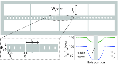
Figure 1: Schematic of the photonic crystal paddle nanocavity (top-view). The paddle is separated from photonic crystal nanobeam mirrors by gaps $d=50$ nm, and has length $L=958$ nm. The elliptical hole horizontal and vertical semi-axes ($R_{x},R_{y}$) are tapered as shown.

The optomechanical device studied here, illustrated in Fig. 1, is a photonic crystal “paddle nanocavity” which combines operating principles of MiM cavities ref:thompson2008sdc ; ref:jayich2008dom and photonic crystal nanobeam optomechanical devices ref:eichenfield2009oc . The device is designed to be fabricated from silicon-on-insulator (refractive index $n_{\text{Si}}=3.48$, thickness $t=220$ nm), and to support modes near $\lambda\sim 1550$ nm. A “paddle” element is suspended within the optical mode of the nanocavity defined by two photonic crystal nanobeam mirrors. The width of the gap ($d=50$ nm) separating the mirrors from the paddle is chosen for smooth variation in local effective-index of the structure ref:hryciw2013ods , and the paddle length ($L=958$ nm) is set to $\approx 1.5\lambda/n_{\text{eff}}$ ref:quan2010pcn . This allows the nanocavity to support high optical quality factor ($Q_{o}$) modes. The length ($l_{s}$) and width ($w_{s}$) of the paddle supports can be adjusted to tailor its mechanical properties, although $l_{s}\geq 200$ nm and $w_{s}\leq 200$ nm is required to not degrade $Q_{o}$. We consider three support geometries, labeled $p1-p3$ (see 2 for dimentions). All of these dimensions are realizable experimentally ref:wu2014ddo .

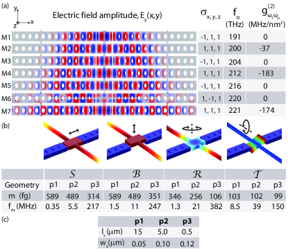
Figure 2: (a) Properties of the localized optical modes of the paddle nanocavity (labeled M1 – M7): electric field distribution ($E_{y}$ component), spatial symmetry in $x-y$ plane, optical frequency, and contribution $g^{(2)}_{\omega_{1}\omega_{n}}$ to the quadratic optomechanical coupling $g^{(2)}$ describing interaction between mode M1 and the $\cal{S}$ mechanical resonance shown in (b). (b) Displacement profiles and properties of the paddle nanocavity mechanical resonances. $m$ and $f_{m}$ are indicated for three support geometries, $p1-p3$, whose cross-sections are given in (c).

Figure 2(a) shows the first seven localized optical modes supported by the paddle nanocavity, calculated using finite element simulations (FEM) footnote . The lowest order mode ($M1$) has a resonance wavelength near 1550 nm ($\omega_{o}/2\pi=191$ THz) and $Q_{o}>1.3\times 10^{4}$. The mechanical resonances of the paddle nanocavity were also calculated using FEM simulations, and the displacement profiles of the four lowest mechanical frequency resonances are shown in Fig. 2(b). They are referred to here as “sliding” ($\cal{S}$), “bouncing” ($\cal{B}$), “rotational” ($\cal{R}$) and “torsional” ($\cal{T}$) resonances. As discussed below, we are particularly interested in the $\cal{S}$ resonance, whose frequency and effective mass ref:eichenfield2009mdc varies between $f_{m}=0.35-217\,$MHz and $m=314-589\,$fg for the support geometries $p1-p3$, as described in Fig. 2(b). Appropriate selection of geometry $p1-p3$ depends on the application, with $p1$ suited for sensitive actuation, $p2$ a compromise between ease of fabrication and sensitivity, and $p3$ for high frequency operation and low thermal phonon occupation.

The spatial symmetry of the nanocavity results in vanishing $g^{(1)}$ for the mechanical resonances considered here. The intensity $E^{2}(x,y,z)$ of each nanocavity optical mode has even symmetry, denoted $\sigma_{x,y,z}=1$, while the mechanical resonances induce perturbation $\Delta\epsilon$ which is odd in at least one direction, characterized by $\sigma_{x}=-1$ ($\cal{S},\cal{R}$), $\sigma_{y}=-1$ ($\cal{R}$) or $\sigma_{z}=-1$ ($\cal{B},\cal{T}$). As a result, $g^{(1)}\propto\langle E_{\omega}|\delta\epsilon|E_{\omega}\rangle=0$. Similarly, the second order self–overlap term in Eq. (1) is also zero. However, the electric field amplitude $E(x,y,z)$ may be even or odd, resulting in non–zero cross-coupling $g^{(2)}_{\omega^{\prime},\omega}$ between optical modes with opposite $\sigma_{x,y,z}$. For example, displacement in the $\hat{x}$ direction of $\cal{S}$ couples optical modes with opposite $\sigma_{x}$. In contrast, displacement in the $\hat{z}$ direction by the $\cal{B}$ and $\cal{T}$ resonances does not induce cross–coupling, as the localized optical modes all have even vertical symmetry ($\sigma_{z}=1$). Here we focus on the nonlinear coupling between the $\cal{S}$ resonance and the $M1$ mode of the nanocavity.

To evaluate $g^{(2)}_{\omega,\omega^{\prime}}$, the mechanical and optical field profiles were input into Eq. (2). The resulting contributions $g_{\omega_{1}\omega_{n}}^{(2)}$ of each localized mode to $g^{(2)}$ for optomechanical coupling between the $\cal{S}$ resonance and the $M1$ mode are summarized in Fig. 2(a). Contributions from delocalized modes are neglected due to their large mode volume and low overlap. The imaginary part of $\omega_{o}$, which is small for the localized modes whose $Q_{o}>10^{2}$, is also ignored. A total $g^{(2)}/2\pi\approx-400$ MHz/nm² is predicted, which matches with our direct FEM calculations (see Supplementary information). The corresponding single photon to two phonon coupling rate, $\Delta\omega_{o}$ depends on the support geometry. For the most flexible $p1$ geometry, $\Delta\omega_{o}\equiv|g^{(2)}x_{zpf}^{2}|=2\pi\times 16$ Hz, where $x_{zpf}=\sqrt{{\hbar}/{2m\omega_{m}}}$. This $\Delta\omega_{o}$ is about four orders of magnitude higher than typical MiM systems ref:sankey2010stn ; ref:lee2014mod , while the mode spacing is five orders of magnitude higher than other nonlinear optomechanical systems ref:sankey2010stn ; ref:ludwig2012eqn ; ref:hill2013now . The dominant contributions to $g^{(2)}$ arise from cross–coupling between modes $M1\leftrightarrow M4$ and $M1\leftrightarrow M7$ due to strong spatial overlap between their fields and the paddle–nanobeam gaps. Increasing $g^{(2)}$ through additional optimization, for example by concentrating the optical field more strongly in the gap, should be possible.

Given $g^{(2)}$ of the paddle nanocavity, the optical response of the device can be predicted. In experimental applications of optomechanical nanocavities, photons are coupled into and out of the nanocavity using an external waveguide. Mechanical fluctuations, $x(t)$ are monitored via variations, $dT(t)$, of the waveguide transmission, $T$. In the sideband unresolved regime ($\omega_{m}\ll\omega_{o}/Q_{o}$), optomechanical coupling results in a fluctuating waveguide output $dT=G_{1}x(t)+\frac{1}{2}G_{2}x(t)^{2}$, where

$$G_{1} =\frac{dT}{dx}=g^{(1)}\frac{dT}{d\Delta},$$ (3)

$$G_{2} =\frac{d^{2}T}{dx^{2}}=g^{(2)}\frac{dT}{d\Delta}+\left(g^{(1)}\right)^{2}\frac{d^{2}T}{d\Delta^{2}}.$$ (4)

Here $\Delta=\omega-\omega_{o}$ is the detuning between input photons and the nanocavity mode, and $dT/d\Delta$, $d^{2}T/d\Delta^{2}$ are the slope and curvature of the Lorentzian cavity resonance in $T(\Delta)$. Eq. (4) shows that in general, both nonlinear transduction of linear optomechanics and linear transduction of nonlinear optomechanics contribute to the second order signal. The nonlinear mechanical displacement can be measured through photodetection of the waveguide optical output. For input power $P_{i}$, the waveguide output optical power spectral density (PSD) due to transduction of $x^{2}(t)$ is $S_{P}^{(2)}(\omega)=\frac{1}{4}P_{i}^{2}G_{2}^{2}S_{x^{2}}(\omega)$, where $S_{x^{2}}(\omega)$ is the PSD of the $x^{2}$ mechanical motion of the mechanical resonance. To analyze the possibility of observing this signal, it is instructive to consider the scenario of a thermally–driven mechanical resonance. As shown in the Supplementary information and Refs. ref:hauer2015nps ; ref:nunnenkamp2010csq , $S_{x^{2}}(\omega)$ of a resonator in a $\bar{n}$ phonon number thermal state is

$$S_{x^{2}}(\omega)=2x_{zpf}^{4} \left(\frac{2\Gamma(\bar{n}+1)^{2}}{\Gamma^{2}+(\omega-2\omega_{m})^{2}}+\frac{2\Gamma\bar{n}^{2}}{\Gamma^{2}+(\omega+2\omega_{m})^{2}}\right.$$

$$+\left.\frac{8\Gamma\bar{n}(\bar{n}+1)+1}{\Gamma^{2}+\omega^{2}}\right),$$ (5)

where $\Gamma=\omega_{m}/Q_{m}$ and $Q_{m}$ is the mechanical quality factor.

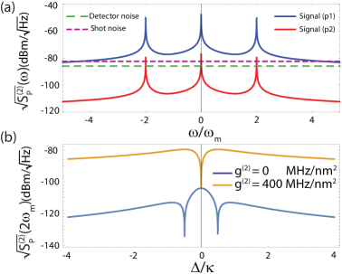
Figure 3: (a) $S_{P}^{(2)}(\omega)$ generated by thermal motion of the $\cal{S}$ mode of a paddle nanocavity for $p1$ and $p2$ support geometry, assuming room temperature operation, $\Delta=\kappa/2$, $P_{i}=100\,\mu$W and $Q_{m}=10^{3}$. (b) $S_{P}^{(2)}(2\omega_{m})$ as a function of detuning $\Delta$, for varying quadratic coupling strengths $g^{(2)}$.

Figure 3 shows $S_{P}^{(2)}(\omega)$ predicted from Eq. (5), for the $\cal{S}$ mode of a paddle nanocavity at room temperature ($T_{b}=300$K). The input optical field is set to $P_{i}=100$ $\mu$W, with detuning $\Delta=\kappa/2$ to maximize the nonlinear optomechanical coupling contribution. The predicted $S_{P}^{(2)}(\omega)$ is shown for $p1$ and $p2$ support geometries, assuming $Q_{m}=10^{3}$, $Q_{o}=1.4\times 10^{4}$, and relatively weak fiber coupling $T_{o}=0.90$. Note that $Q_{m}$ is specified assuming the device is operating in moderate vacuum conditions ref:wu2014ddo , and can increase to $10^{5}$ in cryogenic vacuum conditions ref:safavi2013sls . Also shown are estimated noise levels, assuming direct photodetection using a Newport 1811 photoreceiver (NEP=$2.5$ pW/$\sqrt{Hz}$). Resonances in $S_{P}^{(2)}$ are evident at $\omega=2\omega_{m}$ and $\omega=0$, corresponding to energies of the two phonon processes characteristic of $x^{2}$ optomechanical coupling. Figure 3 suggests that even for these relatively modest device parameters, the nonlinear signal at $2\omega_{m}$ is observable. This signal can be further enhanced with improved device performance. For example, if $Q_{m}=10^{4}$, the nonlinear signal is visible for temperatures as low as 50 mK for the $p1$ geometry. Note that additional technical noise will increase as $f_{m}$ is further decreased into the kHz range.

Nonlinear optomechanical coupling can be differentiated from nonlinear transduction by the $\Delta$ dependence of the nonlinear signal. This is demonstrated in Fig. 3, which shows $S_{P}^{(2)}(2\omega_{m},\Delta)$ with and without quadratic coupling, assuming that fabrication imperfections introduce nominal $g^{(1)}/2\pi=50$ MHz/nm. This demonstrates that at $\Delta=\kappa/2$, the nonlinear signal is dominantly from nonlinear optomechanical coupling.

Next we study the feasibility of QND phonon measurement using a paddle nanocavity. High $\omega_{m}$ is advantageous for ground state cooling which is required for QND measurements. The large optical mode spacing of the paddle nanocavity allows this without introducing Zener tunneling effects ref:ludwig2012eqn or parasitic linear coupling and resulting backaction ref:miao2009sql . Cryogenic temperature of $10$ mK could directly cool the $\cal{S}$ resonance of the $p3$ structure to its quantum ground state. For feasible optical and mechanical quality factors $Q_{o}=10^{6}$ ref:hryciw2013ods ; ref:chan2011lcn and $Q_{m}=10^{5}$ ref:safavi2013sls , the signal to noise ratio (SNR) introduced in Ref. ref:thompson2008sdc of a quantum jump measurement in such a device is $\Sigma^{(0)}=\tau^{(0)}_{tot}\Delta\omega_{0}^{2}/S_{\omega_{o}}=6.4\times 10^{-8}$. Here $\tau^{(0)}_{tot}$ is the thermal lifetime quantifying the rate of decoherence due to bath phonons of the ground state cooled nanomechanical resonator, and $S_{\omega_{o}}$ is the shot noise limited sensitivity of an ideal Pound-Drever-Hall detector. Introducing laser cooling would potentially allow preparation of the $p1$ device to its quantum ground state, where the larger $x_{zpf}$ and $\Delta\omega_{o}$ increases $\Sigma^{(0)}$ to ${2.1\times 10^{-5}}$. However, this would require development of sideband unresolved nonlinear optomechanical cooling ref:nunnenkamp2010csq .

A more feasible approach for observing discreteness of the paddle nanocavity mechanical energy is a QND measurement of phonon shot noise ref:clerk2010qmp . The SNR of such a measurement scales with the magnitude of an applied drive, which enhances the signal by $S=8n_{d}\bar{n}\Sigma^{(0)}$, where $n_{d}$ is the drive amplitude in units of phonon number, and $\bar{n}<1$ for a resonator in the quantum ground state. Using a $p3$ structure, SNR of above one is achievable assuming a drive amplitude of $62$ pm ($n_{d}\approx 7.8\times 10^{6}$) and thermal bath phonon number $\bar{n}=1/4$.

In conclusion, we have designed a single–mode nonlinear optomechanical nanocavity with THz mode spacing. The quadratic optomechanical coupling coefficient $g^{(2)}/2\pi=400$ MHz/nm² and single photon to two phonon coupling rate $\Delta\omega_{0}/2\pi=16$ Hz of this system are among the largest single–mode quadratic optomechanical couplings predicted to-date. Observing a thermal nonlinear signal from this structure is possible in realistic conditions, and a continuous QND measurements of phonon shot noise may be achievable for optimized device parameters.

Funding Information

Natural Science and Engineering Research Council of Canada, Canada Foundation for Innovation, Alberta Innovates Technology Futures, WWTF, Austrian Science Fund (FWF) through SFB FOQUS and the START grant Y 591-N16.

Supplementary Information for “Nonlinear optomechanical paddle nanocavities”

I Evaluation of the nonlinear optomechanical coupling coefficient

The matrix element used in the perturbation theory calculation of $g^{(2)}$ is a measure of the overlap of the nanocavity optical fields and the shifting dielectric boundaries of the mechanical resonance. It is discussed in detail in Refs. sref:johnson2002ptm ; sref:eichenfield2009mdc ; sref:rodriguez2011bat , and is given by

$$\langle E_{\omega^{\prime}}|\frac{\delta\epsilon}{\delta x}|E_{\omega}\rangle=\int\text{d}A({\bf q\cdot\hat{n}})\left[\Delta\epsilon\,\textbf{e}^{\parallel}_{\omega^{\prime}}\cdot\textbf{e}^{*\parallel}_{\omega}-\Delta(\epsilon^{-1})\,\textbf{d}^{\perp}_{\omega^{\prime}}\cdot\textbf{d}^{*\perp}_{\omega}\right]$$ (S1)

where the integral is evaluated over the surface of the nanocavity, and $\textbf{e}^{\parallel}_{\omega}$ and $\textbf{d}^{\perp}_{\omega}$ are the components of the the optical mode electric and displacement fields parallel and perpendicular to the surface, respectively. The perturbation introduced by the mechanical resonance is described by the normalized displacement of the dielectric boundaries, $\textbf{q}=\textbf{Q(r)}/|\textbf{Q(r)}|_{\text{max}}$ where $\textbf{Q}(r)$ is the vectorial displacement field. For the device studied here, the dielectric contrast is constant, and is described by $\Delta\epsilon=\epsilon_{1}-\epsilon_{2}$ and $\Delta(\epsilon^{-1})=1/\epsilon_{2}-1/\epsilon_{1}$ , where $\epsilon_{1}$ is the dielectric constant of the nanocavity, and $\epsilon_{2}=1$ is the dielectric constant of the surrounding medium.

II Nonlinear optomechanical signal

Here we analyze the optical power spectrum generated by a thermally driven mechanical oscillator quadratically coupled to an optical nanocavity. As described by Eq. (5) in the main text, the optical energy spectrum of a quadratically coupled mechanical resonator in a cavity optomechanical system can be written in terms of the autocorrelation of displacement squared,

$$S_{x^{2}}(\omega)=\int_{-\infty}^{+\infty}\langle x^{2}(t)x^{2}(0)\rangle e^{-i\omega t}dt.$$ (S2)

Expressing the displacement in terms of annihilation and creation operators $b$ and $b^{\dagger}$ as $x=x_{zpf}(be^{i\omega_{m}t}+b^{\dagger}e^{-i\omega_{m}t})$ and substituting the displacement operator into Eq. (S2) yields

$$S_{x^{2}}( \omega)=2\pi x_{zpf}^{4}\left[(2(\bar{n}+1)^{2}\delta(\omega-2\omega_{m})\right.$$

$$+\left.2\bar{n}^{2}\delta(\omega+2\omega_{m})+(8\bar{n}(\bar{n}+1)+1)\delta(\omega)\right].$$ (S3)

where $\bar{n}$ is the mean thermal phonon number and $T_{b}$ is the bath temperature. For large phonon numbers $\bar{n}\gg 1$, it is approximated by $\bar{n}=k_{b}T_{b}/\hbar\omega_{m}$ and the area under the nonlinear spectrum is given by

$$\int^{+\infty}_{-\infty}S_{x^{2}}\frac{d\omega}{2\pi}=12\bar{n}x_{zpf}^{4}=3\left(\frac{k_{b}T_{b}}{m\omega_{m}^{2}}\right)^{2}$$ (S4)

which is in agreement with the moment relation for a thermal distribution $\langle x^{4}\rangle=3\langle x^{2}\rangle^{2}$ sref:kardar2007spp . For low loss mechanical resonators ($\Gamma\ll\omega_{m}$) we can replace the delta functions with a Lorentzian $\delta(\omega-\omega_{m})=\frac{1}{\pi}\frac{\Gamma}{\Gamma^{2}+(\omega-\omega_{m})^{2}}$, resulting in the following formula for power spectral density,

$$S_{x^{2}}(\omega)=2x_{zpf}^{4} \left(\frac{2\Gamma(\bar{n}+1)^{2}}{\Gamma^{2}+(\omega-2\omega_{m})^{2}}+\frac{2\Gamma\bar{n}^{2}}{\Gamma^{2}+(\omega+2\omega_{m})^{2}}\right.$$

$$\left.+\frac{8\Gamma\bar{n}(\bar{n}+1)+1}{\Gamma^{2}+\omega^{2}}\right).$$ (S5)

Assuming a large thermal phonon occupancy ($\bar{n}\gg 1$), for frequencies near the double mechanical frequency ($\omega\approx 2\omega_{m}$) we obtain following normalized form (using Eq. (S4)) for nonlinear power spectral density

$$S_{x^{2}}(\omega) =96\left(\frac{k_{B}T_{b}}{m}\right)^{2}\frac{\omega_{m}}{Q_{m}}\times$$

$${\frac{1}{[(\omega^{2}-4\omega_{m}^{2})^{2}+(\frac{2\omega_{m}\omega}{Q_{m}})^{2}][\omega^{2}+(\frac{\omega_{m}}{2Q_{m}})^{2}]}}$$ (S6)

One obtains a similar result from a classical analysis which assumes that during the mechanical decay time, $\Delta t\approx 1/\Gamma$, the thermal force acts as a delta function “kick”. In this approximation, the spectral density of the thermal force is given by sref:saulson1990tnm

$$S_{FF}(\omega)=\frac{|F(\omega)|^{2}}{\Delta t}=\frac{2k_{B}T_{b}m\omega_{m}}{Q_{m}}$$ (S7)

For a measurement time on the order of $\Delta t$,

$$F(\omega)=\sqrt{\frac{2k_{B}T_{b}m\omega_{m}\Delta t}{Q_{m}}}$$ (S8)

and

$$x(\omega)=\sqrt{\frac{2k_{B}T_{b}\omega_{m}\Delta t}{mQ_{m}}}\frac{1}{\omega_{m}^{2}-\omega^{2}+i\Gamma\omega}$$ (S9)

From Eq. (S9) and Eq. (S2), and using the convolution properties of Fourier transforms, we find

$$S_{x^{2}} =96\left(\frac{k_{B}T_{b}}{m}\right)^{2}\frac{\omega_{m}}{Q_{m}}\times$$

$${\frac{1}{[(\omega^{2}-4\omega_{m}^{2})^{2}+(\frac{2\omega_{m}\omega}{Q_{m}})^{2}][\omega^{2}+(\frac{\omega_{m}}{2Q_{m}})^{2}]}},$$ (S10)

after imposing the normalization given by Eq. (S4). As illustrated in Fig. S1, the classical nonlinear signal described by Eq. (S10) matches the quantum result of Eq. (S5) when $\bar{n}\gg 1$, in the neighbourhood of $\omega\sim 2\omega_{m}$. This analysis is in agreement with results in Ref. sref:hauer2015nps .

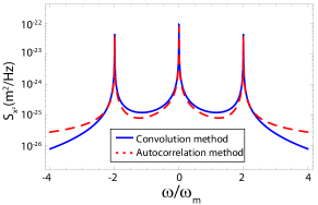
Figure S1: Comparison of the power spectral density of the nonlinear signal obtained from exact autocorrelation analysis resulting in expression Eq. (S5) (red) and the approximate thermal analysis resulting in Eq. (S10) (blue), assuming $\omega_{m}=2\pi\times 5.5$ MHz, $Q_{m}=1000$, and $T_{b}=300$K.

III Validating the second order perturbation theory

The accuracy of the second order perturbation theory, whose use has not been previously reported for nanophotonic cavity–optomechanical devices to the best of our knowledge, was tested by comparing its results with FEM calculations of $\omega_{o}(x)$, Here $x$ parameterizes the paddle displacement from the center position between the two mirrors of the simulated structure. This displacement closely approximates the motion of the $\cal{S}$ resonance which we are primarily interested in here.

This comparison is shown in Fig. S2, where we find good agreement for displacements $|x|\leq 2$ nm, and deviation for larger displacements as the perturbation condition breaks down. This agreement confirms the validity of the assumptions underlying the second order perturbation theory. It also highlights the suitability of this method, as extracting $g^{(2)}$ from parameterized FEM simulations has considerable uncertainty due a $2$ nm minimum mesh available with our computation tool.

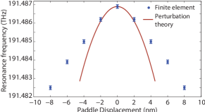
Figure S2: Frequency of the $M1$ nanocavity mode as a function of paddle displacement along the $x$-axis, calculated using FEM simulations of $\omega_{o}(x)$ (data points) and perturbation theory prediction $\omega_{o}(x)=\omega_{o}(0)+(1/2)g^{(2)}x^{2}$ (solid line) with $g^{(2)}/2\pi=400\,\text{MHz/nm}^{2}$. Error bars determined by the lowest significant digit of $\omega_{o}$.

References

- (1) M. Aspelmeyer, T. J. Kippenberg, and F. Marquardt, “Cavity optomechanics,” Rev. Mod. Phys. 86, 1391–1452 (2014).
- (2) M. Eichenfield, J. Chan, R. Camacho, K. Vahala, and O. Painter, “Optomechanical crystals,” Nature 462, 78–82 (2009).
- (3) E. Gavartin, P. Verlot, and T. J. Kippenberg, “A hybrid on-chip optomechanical transducer for ultrasensitive force measurements,” Nat. Nano. 7, 509–514 (2012).
- (4) A. G. Krause, M. Winger, T. D. Blasius, W. Lin, and O. Painter, “A high-resolution microchip optomechanical accelerometer,” Nat. Photon. 6, 768–772 (2012).
- (5) Y. Liu, H. Miao, V. Aksyuk, and K. Srinivasan, “Wide cantilever stiffness range cavity optomechanical sensors for atomic force microscopy,” Opt. Express 20, 18268–18280 (2012).
- (6) X. Sun, J. Zhang, M. Poot, C. W. Wong, and H. X. Tang, “Femtogram doubly clamped nanomechanical resonators embedded in a high-q two-dimensional photonic crystal nanocavity,” Nano Lett. 12, 2299–2305 (2012).
- (7) M. Wu, A. C. Hryciw, C. Healey, D. P. Lake, H. Jayakumar, M. R. Freeman, J. P. Davis, and P. E. Barclay, “Dissipative and dispersive optomechanics in a nanocavity torque sensor,” Phys. Rev. X 4, 021052 (2014).
- (8) J. Chan, T. P. M. Alegre, A. H. Safavi-Naeini, J. T. Hill, A. Krause, S. Groblacher, M. Aspelmeyer, and O. Painter, “Laser cooling of a nanomechanical oscillator into its quantum ground state,” Nature 478, 89–92 (2011).
- (9) A. H. Safavi-Naeini, S. Gröblacher, J. T. Hill, J. Chan, M. Aspelmeyer, and O. Painter, “Squeezed light from a silicon micromechanical resonator,” 500, 185–189 (2013).
- (10) J. D. Thompson, B. M. Zwickl, A. M. Jayich, F. Marquardt, S. M. Girvin, and J. G. E. Harris, “Strong dispersive coupling of a high-finesse cavity to a micromechanical membrane,” Nature 452, 72 (2008).
- (11) A. A. Clerk, F. Marquardt, and J. G. E. Harris, “Quantum measurement of phonon shot noise,” Phys. Rev. Lett. 104, 213603 (2010).
- (12) G. A. Brawley, M. R. Vanner, P. E. Larsen, S. Schmid, A. Boisen, and W. P. Bowen, “Non-linear optomechanical measurement of mechanical motion,” arXiv preprint arXiv:1404.5746 (2014).
- (13) M. Ludwig, A. H. Safavi-Naeini, O. Painter, and F. Marquardt, “Enhanced quantum nonlinearities in a two-mode optomechanical system,” Phys. Rev. Lett. 109, 063601 (2012).
- (14) M. Bhattacharya, H. Uys, and P. Meystre, “Optomechanical trapping and cooling of partially reflective mirrors,” Physical Review A 77, 033819 (2008).
- (15) A. Nunnenkamp, K. Børkje, J. G. E. Harris, and S. M. Girvin, “Cooling and squeezing via quadratic optomechanical coupling,” Phys. Rev. A 82, 021806 (2010).
- (16) C. Biancofiore, M. Karuza, M. Galassi, R. Natali, P. Tombesi, G. Di Giuseppe, and D. Vitali, “Quantum dynamics of an optical cavity coupled to a thin semitransparent membrane: Effect of membrane absorption,” Physical Review A 84, 033814 (2011).
- (17) J.-Q. Liao and F. Nori, “Single-photon quadratic optomechanics,” Scientific Reports 4 (2014).
- (18) J. C. Sankey, C. Yang, B. M. Zwickl, A. M. Jayich, and J. G. E. Harris, “Strong and tunable nonlinear optomechanical coupling in a low-loss system,” Nature Phys. 6, 707–712 (2010).
- (19) N. Flowers-Jacobs, S. Hoch, J. Sankey, A. Kashkanova, A. Jayich, C. Deutsch, J. Reichel, and J. Harris, “Fiber-cavity-based optomechanical device,” Applied Physics Letters 101, 221109 (2012).
- (20) M. Karuza, M. Galassi, C. Biancofiore, C. Molinelli, R. Natali, P. Tombesi, G. Di Giuseppe, and D. Vitali, “Tunable linear and quadratic optomechanical coupling for a tilted membrane within an optical cavity: theory and experiment,” Journal of Optics 15, 025704 (2013).
- (21) D. Lee, M. Underwood, D. Mason, A. Shkarin, S. Hoch, and J. Harris, “Multimode optomechanical dynamics in a cavity with avoided crossings,” arXiv:1401.2968 (2014).
- (22) J. T. Hill, “Nonlinear optics and wavelength translation via cavity-optomechanics,” PhD Thesis (2013).
- (23) C. Doolin, B. Hauer, P. Kim, A. MacDonald, H. Ramp, and J. Davis, “Nonlinear optomechanics in the stationary regime,” Physical Review A 89, 053838 (2014).
- (24) G. Heinrich, J. Harris, and F. Marquardt, “Photon shuttle: Landau-zener-stückelberg dynamics in an optomechanical system,” Physical Review A 81, 011801 (2010).
- (25) H. Miao, S. Danilishin, T. Corbitt, and Y. Chen, “Standard quantum limit for probing mechanical energy quantization,” Phys. Rev. Lett. 103, 100402 (2009).
- (26) S. G. Johnson, M. Ibanescu, M. A. Skorobogatiy, O. Weisberg, J. D. Joannopoulos, and Y. Fink, “Perturbation theory for Maxwell’s equations with shifting material boundaries,” Phys. Rev. E 65, 066611 (2002).
- (27) A. W. Rodriguez, A. P. McCauley, P.-C. Hui, D. Woolf, E. Iwase, F. Capasso, M. Loncar, and S. G. Johnson, “Bonding, antibonding and tunable optical forces in asymmetric membranes,” Opt. Express 19, 2225–2241 (2011).
- (28) M. Eichenfield, J. Chan, A. H. Safavi-Naeini, K. J. Vahala, and O. Painter, “Modeling dispersive coupling and losses of localized optical and mechanical modes in optomechanical crystals,” Opt. Express 17, 20078–20098 (2009).
- (29) A. Jayich, J. Sankey, B. Zwickl, C. Yang, J. Thompson, S. Girvin, A. Clerk, F. Marquardt, and J. Harris, “Dispersive optomechanics: a membrane inside a cavity,” New Journal of Physics 10, 095008 (2008).
- (30) A. C. Hryciw and P. E. Barclay, “Optical design of split-beam photonic crystal nanocavities,” Opt. Lett. 38, 1612–1614 (2013).
- (31) Q. Quan, P. B. Deotare, and M. Loncar, “Photonic crystal nanobeam cavity strongly coupled to the feeding waveguide,” Applied Physics Letters 96, 203102 (2010).
- (32) COMSOL software was used for all FEM simulations.
- (33) B. Hauer, J. Maciejko, and J. Davis, “Nonlinear power spectral densities for the harmonic oscillator,” arXiv preprint arXiv:1502.02372 (2015).

References

- (1) S. G. Johnson, M. Ibanescu, M. A. Skorobogatiy, O. Weisberg, J. D. Joannopoulos, and Y. Fink, “Perturbation theory for Maxwell’s equations with shifting material boundaries,” Phys. Rev. E 65, 066611 (2002).
- (2) M. Eichenfield, J. Chan, A. H. Safavi-Naeini, K. J. Vahala, and O. Painter, “Modeling dispersive coupling and losses of localized optical and mechanical modes in optomechanical crystals,” Opt. Express 17, 20078–20098 (2009).
- (3) A. W. Rodriguez, A. P. McCauley, P.-C. Hui, D. Woolf, E. Iwase, F. Capasso, M. Loncar, and S. G. Johnson, “Bonding, antibonding and tunable optical forces in asymmetric membranes,” Opt. Express 19, 2225–2241 (2011).
- (4) M. Kardar, Statistical Physics of Particles (Cambridge university press, 2007).
- (5) P. R. Saulson, “Thermal noise in mechanical experiments,” Phys. Rev. D 42, 2437–2445 (1990).
- (6) B. Hauer, J. Maciejko, and J. Davis, “Nonlinear power spectral densities for the harmonic oscillator,” arXiv preprint arXiv:1502.02372 (2015).