Dynamics of Information Diffusion and Social Sensing

Abstract

Statistical inference using social sensors is an area that has witnessed remarkable progress in the last decade. It is relevant in a variety of applications including localizing events for targeted advertising, marketing, localization of natural disasters and predicting sentiment of investors in financial markets. This chapter presents a tutorial description of four important aspects of sensing-based information diffusion in social networks from a communications/signal processing perspective. First, diffusion models for information exchange in large scale social networks together with social sensing via social media networks such as Twitter is considered. Second, Bayesian social learning models and risk averse social learning is considered with applications in finance and online reputation systems. Third, the principle of revealed preferences arising in micro-economics theory is used to parse datasets to determine if social sensors are utility maximizers and then determine their utility functions. Finally, the interaction of social sensors with YouTube channel owners is studied using time series analysis methods. All four topics are explained in the context of actual experimental datasets from health networks, social media and psychological experiments. Also, algorithms are given that exploit the above models to infer underlying events based on social sensing. The overview, insights, models and algorithms presented in this chapter stem from recent developments in network science, economics and signal processing. At a deeper level, this chapter considers mean field dynamics of networks, risk averse Bayesian social learning filtering and quickest change detection, data incest in decision making over a directed acyclic graph of social sensors, inverse optimization problems for utility function estimation (revealed preferences) and statistical modeling of interacting social sensors in YouTube social networks.

Keywords. diffusion, Susceptible-Infected-Susceptible (SIS model), random graphs, mean field dynamics, social sampling, social learning, risk averse social learning filter, conditional value at risk, reputation systems, Afriat’s theorem, detecting utility maximizers, revealed preferences, potential games, Granger causality, YouTube

1 Introduction and Motivation

Humans can be viewed as social sensors that interact over a social network to provide information about their environment. Examples of information produced by such social sensors include Twitter posts, Facebook status updates, and ratings on online reputation systems like Yelp and Tripadvisor. Social sensors go beyond physical sensors – for example, user opinions/ratings (such as the quality of a restaurant) are available on Tripadvisor but are difficult to measure via physical sensors. Similarly, future situations revealed by the Facebook status of a user are impossible to predict using physical sensors [161].

Statistical inference using social sensors is an area that has witnessed remarkable progress in the last decade. It is relevant in a variety of applications including localizing special events for targeted advertising [119, 42], marketing  [172, 122], localization of natural disasters [162], and predicting sentiment of investors in financial markets [27, 150]. For example, [15] reports sthat models built from the rate of tweets for particular products can outperform market-based predictors.

1.1 Context: Why social sensors?

Social sensors present unique challenges from a statistical estimation point of view. First, social sensors interact with and influence other social sensors. For example, ratings posted on online reputation systems strongly influence the behavior of individuals. Such interacting sensing can result in non-standard information patterns due to correlations introduced by the structure of the underlying social network. Thus certain events “go viral" [122, 70]. Second, due to privacy concerns and time-constraints, social sensors typically do not reveal raw observations of the underlying state of nature. Instead, they reveal their decisions (ratings, recommendations, votes) which can be viewed as a low resolution (quantized) function of their raw measurements and interactions with other social sensors. This can result in misinformation propagation, herding and information cascades. Third, the response of a social sensors may not be consistent with that of an utility maximizer; social sensors are typically risk averse.

Social sensors are enabled by technological networks. Indeed, social media sites that support interpersonal communication and collaboration using Internet-based social network platforms, are growing rapidly. McKinsey estimates that the economic impact of social media on business is potentially greater than $1 trillion since social media facilitates efficient communication and collaboration within and across organizations.

1.2 Main Results and Organization

There is strong motivation to construct models that facilitate understanding the dynamics of information flow in social networks. This chapter presents a tutorial description of four mportant aspects of sensing-based information diffusion in social networks from a signal processing perspective:

1.2.1 Information Diffusion in Large Scale Social Networks

The first topic considered in this chapter (Sec.2) is diffusion of information in social networks comprised of a population of interacting social sensors. The states of sensors evolve over time as a probabilistic function of the states of their neighbors and an underlying target process. Several recent papers investigate such information diffusion in real-world social networks. Motivated by marketing applications, [167] studies diffusion (contagion) behavior in Facebook. Using data from 260,000 Facebook pages (which advertise products, services and celebrities), [167] analyzes information diffusion. In [159], the spread of hashtags on Twitter is studied. There is a wide range of social phenomena such as diffusion of technological innovations, sentiment, cultural fads, and economic conventions [36, 130] where individual decisions are influenced by the decisions of others.

We consider the so called Susceptible-Infected-Susceptible (SIS) model [151] for information diffusion in a social network. It is shown for social networks comprised of a large number of agents how the dynamics of degree distribution can be approximated by the mean field dynamics. Mean field dynamics have been studied in [21] and applied to social networks in [130] and leads to a tractable model for the dynamics social sensors.

We demonstrate using influenza datasets from the U.S Centers for Disease Control and Prevention (CDC) how Twitter can be used as a real time social sensor for tracking the spread of influenza. That is, a health network (namely, Influenza-like Illness Surveillance Network (ILInet)) is sensed by a real time microblogging social media network (namely, Twitter).

We also review two recent methods for sampling social networks, namely, social sampling and respondent-driven sampling. Respondent-driven sampling is now used by the U.S. Centers for Disease Control and Prevention (CDC) as part of the National HIV Behavioral Surveillance System in health networks.

1.2.2 Bayesian Social Learning in Online Reputation Systems

The second topic of this chapter (Sec.3) considers online reputation systems where individuals make recommendations based on their private observations and recommendations of friends. Such interaction of individuals and their social influence is modelled as Bayesian social learning [18, 25, 36] on a directed acyclic graph. We consider two important classes of such problems; risk averse social learning in financial systems, and data incest in reputation systems. The risk averse social learning and associated quickest change detection is important in detecting market shocks in high frequency trading. Data incest (misinformation propagation) arises as a result of correlations in recommendations due to the intersection of multiple paths in the information exchange graph. Necessary and sufficient conditions are given on the structure of information exchange graph to mitigate data incest. Experimental results on human subjects are presented to illustrate the effect of social influence and data incest on decision making.

The setup differs from classical signal processing where sensors use noisy observations to compute estimates - in social learning agents use noisy observations together with decisions made by previous agents, to estimate the underlying state of nature. Social learning has been used widely in economics, marketing, political science and sociology to model the behavior of financial markets, crowds, social groups and social networks; see [18, 25, 2, 36, 127, 1] and numerous references therein. Related models have been studied in the context of sequential decision making in information theory [45, 84] and statistical signal processing [37, 112] in the electrical engineering literature. Social learning can result in unusual behavior such as herding [25] where agents eventually choosing the same action irrespective of their private observations. As a result, the actions contain no information about the private observations and so the Bayesian estimate of the underlying random variable freezes. Such behavior can be undesirable, particularly if individuals herd and make incorrect decisions.

1.2.3 Revealed Preferences and Detection of Utility Maximizers

The third topic considered in this chapter (Sec.4) is the principle of revealed preferences arising in microeconomics. It is used as a constructive test to determine: Are social sensors utility optimizers in their response to external influence? The key question considered is as follows: Given a time-series of data $\mathcal{D}=\{(p_{t},x_{t}),t\in\{1,2,\dots,T\}\}$ where $p_{t}\in\mathds{R}^{m}$ denotes the external influence, $x_{t}$ denotes the response of an agent, is it possible to detect if the agent is a utility maximizer?

These issues are fundamentally different to the model-centric theme used in the signal processing literature where one postulates an objective function (typically convex) and then proposes optimization algorithms. In contrast the revealed preference approach is data centric - given a dataset, we wish to determine if is consistent with utility maximization.

We present a remarkable result called Afriat’s theorem [7, 175] which provides a necessary and sufficient condition for a finite dataset $\mathcal{D}$ to have originated from a utility maximizer. Also a multi-agent version of Afriat’s theorem is presented to determine if the dataset generated by multiple agents is consistent with playing from the equilibrium of a potential game.

Unlike model centric applications of game theory in signal processing, the revealed preferences approach is data centric: 1) Given a time series dataset of probe and response signals, how can one detect if the response signals are consistent with a Nash equilibrium generated by players in a concave potential game? 2) If consistent with a concave potential game, how can the utility function of the players be estimated?

We present three datasets involving social sensors to illustrate Afriat’s theorem of revealed preferences. These datasets are: (i) an auction conducted by undergraduate students at Princeton University, (ii) aggregate power consumption in the electricity market of Ontario province and (iii) Twitter dataset for specific hashtags.

Varian has written several influential papers on Afriat’s theorem in the economics literature. These include measuring the welfare effect of price discrimination [177], analysing the relationship between prices of broadband Internet access and time of use service [180], and ad auctions for advertisement position placement on page search results from Google [180, 179]. Despite widespread use in economics, revealed preference theory is relatively unknown in the electrical engineering literature.

1.2.4 Social Interaction of YouTube Consumers

The fourth topic considered in this chapter (Sec.5) is the engagement dynamics of social sensors to online video content. Specifically, we consider how users interact with video content created on the YouTube social network. YouTube is the largest user-driven video content provider in the world and has become a major platform for disseminating multimedia information. YouTube contains over 1 billion users who collectively watch millions of hours of YouTube videos and generate billions of views every day (e.g. 150 years of video are watched every day). Additionally, users upload over 300 hours of video content every minute. YouTube generates billions in revenue through advertising and also shares the revenue with the popular users that upload videos through the Partner program. YouTube is clearly a social media site, however is YouTube also a social networking site? In classical online social networks the interaction is directly between users–that is, user-user interactions. However YouTube is unique in that the interaction between users includes video content–that is, the interaction follows users-content-users. In fact the interaction between users is incentivized using the posted videos. In this way it is not merely the interest preferences between users that promote user-user interaction, but also the content of the videos that governs the social interactions between users.

Using real-world data consisting of over $6$ million videos spread over $25$ thousand channels, we empirically examine the sensitivity of YouTube meta-level features on the engagement dynamics of users in YouTube. Insight into the dynamics of social sensors in YouTube can be used to predict how users will interact with posted video content. These results are important for designing methods for optimizing user engagement and for improving the efficiency of content distribution networks [87, 164, 88]. Estimating the popularity of YouTube videos based on meta-level features is a challenging problem given the diversity of users and content providers. Time-series methods for modeling YouTube the engagement dynamics of videos over time include ARMA time series models [75], multivariate linear regression models [153], and Gompertz models [156, 157]. These methods do not utilize any of the meta-level features of the YouTube video to estimate the users engagement dynamics. In [187] a bag-of-words Bernoulli Naive Bayes classifier is applied to perform a binary classification (popular/unpopular) of YouTube videos based on the title alone. The classifier was able to achieve a classification accuracy of 66%. In [87] visual perception and extreme learning machines were applied to the meta-level features of videos and found to be able to accurately estimate the (popular/unpopular) videos with an accuracy of 80%. It was determined that the main meta-level features that impact video engagement include: first day view count , number of subscribers, and contrast of the video thumbnail.

The above methods focus on how to estimate user engagement to specific videos; however, they do not consider the social learning dynamics that are present between users and channel owners. The key topics focused on in Sec.5 are: (i) how user engagement is affected by changes in meta-level (title, thumbnail, tag) features of the videos, (ii) the causal relationship between channel subscribers and user engagement, (iii) the engagement dynamics of videos over time with exogenous social media events, and (iv) the engagement of users to videos in a channel’s video playlist. The insight provided can be used by channel owners to design policies for maximizing user engagement by adjusting video meta-level features, promoting on external social media venues, and periodically adjusting the uploading schedule of videos.

1.3 Perspective

The unifying theme that underpins the four topics in this chapter stems from statistical signal processing and controlled sensing. These are used to predict global behavior given local behavior: individual social sensors interact with other sensors and we are interested in understanding the behavior of the entire network. Information diffusion, social learning and revealed preferences are important issues for social sensors. We treat these issues in a highly stylized manner so as to provide easy accessibility to a signal processing audience. The underlying tools used in this chapter are widely used in signal processing, economics and network science.

Let us briefly discuss how the four themes of this chapter interact; these four themes are depicted in Fig.1.

Figure 1: Four themes considered in this chapter

The network diffusion models are non-Bayesian and describe the behavior of large numbers of social sensors. The mean field dynamics model for the diffusion of information has the form of an averaged stochastic approximation algorithm (which is widely used in adaptive filtering). Note however, here that the stochastic approximation type equation is a generative model, and not an algorithm.

The Bayesian social learning models in contrast describe highly stylized individual behavior of social sensors. At this level, it is important to model risk-averse human decision making and the Bayesian social learning model serves as a useful generative model.

Underpinning both the network diffusion and Bayesian social learning models, are utility (cost) functions which the social sensors optimize in order to make decisions. The natural question is: Given real world data, is the behavior of agents consistent with optimizing a utility function? If yes, can the utility function be estimated? Revealed preferences yield a useful set of algorithms that can answer both these questions. More generally, it can be used to detect play from the Nash equilibrium of a potential game. Put simply, revealed preferences provide the data-driven justification for the utility function models.

Finally, the detailed analysis of the YouTube data provides for an interesting real world study of how social sensors interact. It is important to note that while YouTube is clearly a social media site, it is also a social networking site. Classical online social networks (OSNs) are dominated by user-user interactions. However YouTube is unique in that the interaction between users includes video content?that is, the interaction follows users-content-users. The interaction between users in the YouTube social network is incentivized using the posted videos. In addition to the social incentives, YouTube also gives monetary incentives to promote users increasing their popularity. As more users view and interact with a users video or channel, YouTube will pay the user proportional to the advertisement exposure on the users channel. Therefore, users not only maximize exposure to increase their social popularity, but also for monetary gain which introduce unique dynamics in the formation of edges in the YouTube social network.

Books and Tutorials

The literature in social learning, information diffusion and revealed preferences is extensive. In each of the following sections, we provide a brief review of relevant works. Seminal books in social networks, social learning and network science include [181, 93, 36, 57]. There is a growing literature dealing with the interplay of technological and social networks [40]. Social networks overlaid on technological networks account for a significant fraction of Internet use. As discussed in [40], three key aspects that cut across social and technological networks are the emergence of global coordination through local actions, resource sharing models and the wisdom of crowds. These themes are addressed in the current chapter in the context of social learning, diffusion and revealed preferences. Other tutorials include [113, 109].

2 Information Diffusion in Large Scale Social Networks

This section addresses the first topic of the chapter, namely, information diffusion models and their mean field dynamics in social networks. The setting is as follows: The states of individual nodes in the social network evolve over time as a probabilistic function of the states of their neighbors and an underlying target process (state of nature). The underlying target process can be viewed as the market conditions or competing technologies that evolve with time and affect the information diffusion. The nodes in the social network are sampled randomly to determine their state. As the adoption of the new technology diffuses through the network, its effect is observed via sentiments (such as tweets) of these selected members of the population. These selected nodes act as social sensors. In signal processing terms, the underlying target process can be viewed as a signal, and the social network can be viewed as a sensor. The key difference compared to classical sensing is that the sensor now is a social network with diffusion dynamics and noisy measurements (due to sampling nodes).

As described in Sec.1, a wide range of social phenomena such as diffusion of technological innovations, cultural fads, ideas, behaviors, trends and economic conventions [72, 139, 41, 36] can be modelled by diffusion in social networks. Another important application is sentiment analysis (opinion mining) where the spread of opinions amongst people is monitored via social media.

Motivated by the above setting, this section proceeds as follows:

1. We describe the Susceptible-Infected-Susceptible (SIS) model for diffusion of information in social networks which has been extensively studied in [93, 129, 130, 151, 181].

2. Next, it is shown how the dynamics of the infected degree distribution of the social network can be approximated by the mean field dynamics. The mean field dynamics state that as the number of agents in the social network goes to infinity, the dynamics of the infected degree distribution converges to that of an ordinary differential (or difference) equation. Such averaging theory results are widely used to analyze adaptive filters. For social networks, they yield a useful tractable model for the diffusion dynamics.

3. We illustrate the diffusion model by using data sets from 3 related social networks to track the spread of influenza during the period September 1 to December 31, 2009. The friendship network of 744 undergraduate students at Harvard college is used together with the U.S. outpatient Influenza-like Illness Surveillance Network (ILInet) to monitor the spread of influenza. Then it is shown that Twitter posts related to influenza during this period are correlated with the spread of influenza. Thus in this example, influenza diffuses in a human health network (Harvard friendship network at a local level and ILInet at a global level) and Twitter is used as a social sensor to monitor the spread of the influenza.

4. Finally, this section also describes how social networks can be sampled. We review two recent methods for sampling social networks, namely, social sampling and respondent-driven sampling; the latter being used in health networks.

(a) Dynamics of Health Network impact the # of tweets.

(b) Model for the number of tweets resulting from the Influenza Health Network.

Figure 2: Dynamics of Health Network are modelled using the SIS model and a Linear and Nonlinear Autoregressive with Exogenous input time series models, refer to Sec.2 for details.

The aim is to estimate the underlying target state that is being sensed by the social network and also and the state probabilities of the nodes by sampling measurements at nodes in the social network. In a Bayesian estimation context, this is equivalent to a filtering problem involving estimation of the state of a prohibitively large scale Markov chain in noise. The mean field dynamics yields a tractable approximation with provable bounds for the information diffusion. Such mean field dynamics have been studied in [21] and applied to social networks in [129, 130, 181]. For an excellent recent exposition of interacting particle systems comprising of agents each with a finite state space, see [9], where the more apt term “Finite Markov Information Exchange (FMIE) process” is used.

Regarding real datasets, in addition to the case study presented below, for other examples of diffusion datasets and their analysis see [167, 159]. A repository of social network datasets can be obtained at [121].

2.1 Social Network Model

A social network is modelled as a graph with $N$ vertices:

$$G=(V,E),\text{ where }V=\{1,2,\ldots,{N}\},\text{ and }E\subseteq V\times V.$$ (1)

Here, $V$ denotes the finite set of vertices, and $E$ denotes the set of edges. In social networks, it is customary to use the terminology network, nodes and links for graph, vertices and edges, respectively.

We use the notation $({m},n)$ to refer to a link between node ${m}$ and $n$. The network may be undirected in which case $({m},n)\in E$ implies $(n,{m})\in E$. In undirected graphs, to simplify notation, we use the notation ${m},n$ to denote the undirected link between node $n$ and ${m}$. If the graph is directed, then $({m},n)\in E$ does not imply that $(n,{m})\in E$. We will assume that self loops (reflexive links) of the form $i,i$ are excluded from $E$.

An important parameter of a social network $G=(V,E)$ is the connectivity of its nodes. Let $\mathcal{N}^{({m})}$ and $D^{({m})}$ denote the neighbourhood set and degree (or connectivity) of a node ${m}\in V$, respectively. That is, with $|\cdot|$ denoting cardinality,

$$\mathcal{N}^{({m})}=\{n\in V:{m},n\in E\},\quad D^{({m})}=\big{|}\mathcal{N}^{({m})}\big{|}.$$ (2)

For convenience, we assume that the maximum degree of the network is uniformly bounded by some fixed integer $\bar{D}$.

Let ${N{(d)}}$ denote the number of nodes with degree $d$, and let the degree distribution ${P{(d)}}$ specify the fraction of nodes with degree $d$. That is, for $d=0,1,\ldots,\bar{D}$,

$${N{(d)}}=\sum_{{m}\in V}I\left\{D^{({m})}=d\right\},\quad{P{(d)}}=\frac{{N{(d)}}}{{N}missing}.$$

Here, $I\left\{\cdot\right\}$ denotes the indicator function. Note that $\sum_{d}{P{(d)}}=1$. The degree distribution can be viewed as the probability that a node selected randomly with uniform distribution on $V$ has a connectivity $d$.

Random graphs generated to have a degree distribution ${P}$ that is Poisson were formulated by Erdös and Renyi [59]. Several recent works show that large scale social networks are characterized by connectivity distributions that are different to Poisson distributions. For example, the internet, www have a power law connectivity distribution ${P}(d)\propto d^{-\gamma}$, where $\gamma$ ranges between 2 and 3. Such scale free networks are studied in [19]. In the rest of this chapter, we assume that the degree distribution of the social network is arbitrary but known—allowing an arbitrary degree distribution facilities modelling complex networks.

Let $k=0,1,\ldots$ denote discrete time. Assume the target process ${s}$ is a finite state Markov chain with transition probability

$$A_{ss^{\prime}}=\mathbb{P}\left({s_{k+1}}=s^{\prime}|{s_{k}}=s\right).$$ (3)

In the example of technology diffusion, the target process can denote the availability of competition or market forces that determine whether a node adopts the technology. In the model below, the target state will affect the probability that an agent adopts the new technology.

2.2 SIS Diffusion Model for Information in Social Network

The model we present below for the diffusion of information in the social network is called the Susceptible-Infected-Susceptible (SIS) model [151, 181]. The diffusion of information is modelled by the time evolution of the state of individual nodes in the network. Let $x_{k}^{({m})}\in\{0,1\}$ denote the state at time $k$ of each node ${m}$ in the social network. Here, $x_{k}^{({m})}=0$ if the agent at time $k$ is susceptible and $x_{k}^{({m})}=1$ if the agent is infected. At time $k$, the state vector of the ${N}$ nodes is

$$x_{k}=\left[x_{k}^{(1)},\ldots,x_{k}^{({N})}\right]^{\prime}\in\{0,1\}^{{N}}.$$ (4)

Assume that the process $x$ evolves as a discrete time Markov process with transition law depending on the target state ${s}$. If node ${m}$ has degree $D^{({m})}=d$, then the probability of node ${m}$ switching from state $i$ to $j$ is

$$\mathbb{P}\left(x_{k+1}^{({m})}=j|x_{k}^{({m})}=i,x_{k}^{(i-)},{s_{k}}=s\right)=p_{ij}(d,A^{({m})}_{k},s),\;i,j\in\{0,1\}.$$ (5)

Here, $A^{({m})}_{k}$ denotes the number of infected neighbors of node ${m}$ at time $k$. That is,

$$A^{({m})}_{k}=\sum_{n\in N^{({m})}}I\left\{n:x_{k}^{({m})}=1\right\}.$$ (6)

In words, the transition probability of an agent depends on its degree distribution and the number of active neighbors.

With the above probabilistic model, we are interested in modelling the evolution of infected agents over time. Let $\rho_{k}(d)$ denote the fraction of infected nodes at each time $k$ with degree $d$. We call $\rho$ the infected node distribution. So with $d=0,1,\ldots,\bar{D}$,

$$\rho_{k}(d)=\frac{1}{{N}(d)}\sum_{{m}\in V}I\left\{D^{({m})}=d,x_{k}^{({m})}=1\right\}.$$ (7)

The SIS model assumes that the infection spreads according to the following dynamics:

1. At each time instant $k$, a single agent, denoted by ${m}$, amongst the ${N}$ agents is chosen uniformly. Therefore, the probability that the chosen agent ${m}$ is infected and of degree $d$ is $\rho_{k}(d)\,{P{(d)}}$. The probability that the chosen agent ${m}$ is susceptible and of degree $d$ is $(1-\rho_{k}(d))\,{P{(d)}}$.

2. Depending on whether its state $x_{k}^{({m})}$ is infected or susceptible, the state of agent ${m}$ evolves according to the transition probabilities specified in (5).

With the Markov chain transition dynamics of individual agents specified above, it is clear that the infected distribution $\rho_{k}=\big{(}\rho_{k}(1),\ldots,\rho_{k}(\bar{D})\big{)}$ is an $\prod_{d=1}^{\bar{D}}{N{(d)}}$ state Markov chain. Indeed, given $\rho_{k}(d)$, due to the infection dynamics specified above

$$\rho_{k+1}(d)\in\left\{\rho_{k}(d)-\frac{1}{{N{(d)}}},\;\rho_{k}(d)+\frac{1}{{N{(d)}}}\right\}.$$ (8)

Our aim below is to specify the transition probabilities of the Markov chain $\rho$. Let us start with the following statistic that forms a convenient parametrization of the transition probabilities. Given the infected node distribution $\rho_{k}$ at time $k$, define $\theta(\rho_{k})$ as the probability that at time $k$ a uniformly sampled link in the network points to an infected node. We call $\theta(\rho_{k})$ as the infected link probability. Clearly

$$\theta(\rho_{k}) =\frac{\sum_{d=1}^{\bar{D}}\text{(\# of links from infected node of degree $d$)}}{\sum_{d=1}^{\bar{D}}\text{(\# of links of degree $d$)}}$$

$$=\frac{\sum_{d=1}^{\bar{D}}d\,{P{(d)}}\,\rho_{k}(d)}{\sum_{d}^{\bar{D}}d\,{P{(d)}}}.$$ (9)

In terms of the infected link probabilities, the scaled transition probabilities of the process $\rho$ are:

$${\bar{p}_{01}(d,\theta_{k},s)} \stackrel{{\scriptstyle\text{defn}}}{{=}}\frac{1}{{P{(d)}}}\,\mathbb{P}\left(\rho_{k+1}(d)=\rho_{k}(d)+\frac{1}{{N{(d)}}}\Big{|}{s_{k}}=s\right)$$

$$=(1-\rho_{k}(d))\,\sum_{a=0}^{d}p_{01}(d,a,s)\,\mathbb{P}(\text{$a$ out of $l$ neighbours infected})$$

$$=(1-\rho_{k}(d))\,\sum_{a=0}^{d}p_{01}(d,a,s)\binom{d}{a}\theta_{k}^{a}(1-\theta_{k})^{d-a},$$

$${\bar{p}_{10}(d,\theta_{k},s)} \stackrel{{\scriptstyle\text{defn}}}{{=}}\frac{1}{{P{(d)}}}\,\mathbb{P}\left(\rho_{k+1}(d)=\rho_{k}(d)-\frac{1}{{N{(d)}}}\Big{|}{s_{k}}=s\right)$$

$$=\rho_{k}(d)\,\sum_{a=0}^{d}p_{10}(d,a,s)\,\binom{d}{a}\theta_{k}^{a}(1-\theta_{k})^{d-a}.$$ (10)

In the above, the notation $\theta_{k}$ is the short form for $\theta(\rho_{k})$. The transition probabilities ${\bar{p}}_{01}$ and ${\bar{p}}_{10}$ defined above model the diffusion of information about the target state ${s}$ over the social network. We have the following martingale representation theorem for the evolution of Markov process $\rho$.

Let $\mathcal{F}_{k}$ denote the sigma algebra generated by $\{\rho_{0},\dots,\rho_{k},{s_{0}},\ldots{s_{k}}\}$.

Theorem 2.1.

For $d=1,2,\ldots,\bar{D}$, the infected distributions evolve as

$$\rho_{k+1}(d)=\rho_{k}(d)+\frac{1}{{N}missing}\bigl{[}{\bar{p}_{01}(d,\theta(\rho_{k}),{s_{k}})}-{\bar{p}_{10}(d,\theta(\rho_{k}),{s_{k}})}+w_{k+1}\bigr{]}$$ (11)

where $w$ is a martingale increment process, that is $\mathbf{E}\{w_{k+1}|\mathcal{F}_{k}\}=0$. Recall ${s}$ is the finite state Markov chain that models the target process. ∎

The above theorem is a well-known martingale representation of a Markov chain [58]—it says that a discrete time Markov process can be obtained by discrete time filtering of a martingale increment process. The theorem implies that the infected distribution dynamics resemble what is commonly called a stochastic approximation (adaptive filtering) algorithm in statistical signal processing: the new estimate is the old estimate plus a noisy update (the “noise” being a martingale increment) that is weighed by a small step size $1/{N}$ when ${N}$ is large. Subsequently, we will exploit the structure in Theorem 2.1 to devise a mean field dynamics model which has a state of dimension $\bar{D}$. This is to be compared with the intractable state dimension $\prod_{d=1}^{\bar{D}}{N{(d)}}$ of the Markov chain $\rho$.

2.3 Mean Field Dynamics of Information Diffusion

The mean field dynamics state that as the number of agents ${N}$ grows to infinity, the dynamics of the infected distribution $\rho$, described by (11), in the social network evolves according to the following deterministic difference equation that is modulated by a Markov chain that depends on the target state evolution ${s}$:

For $d=1,2,\ldots,\bar{D}$,

$$\bar{\rho}_{k+1}(d) =\bar{\rho}_{k}(d)+\frac{1}{{N}missing}\bigl{[}{\bar{p}_{01}(d,\theta(\bar{\rho}_{k}),{s_{k}})}-{\bar{p}_{10}(d,\theta(\bar{\rho}_{k}),{s_{k}})}\bigr{]}$$

$${\bar{p}_{01}(d,\theta,{s_{k}})} =(1-\bar{\rho}_{k}(d))\sum_{a=0}^{d}p_{01}(d,a,{s_{k}})\binom{d}{a}\theta^{a}(1-\theta)^{d-a}$$

$${\bar{p}_{10}(d,\theta,{s_{k}})} =\bar{\rho}_{k}(d)\,\sum_{a=0}^{d}p_{10}(d,a,{s_{k}})\binom{d}{a}\theta^{a}(1-\theta)^{d-a}$$

$$\theta(\bar{\rho}_{k}) =\frac{\sum_{d=1}^{\bar{D}}d\,{P{(d)}}\,\bar{\rho}_{k}(d)}{\sum_{d}^{\bar{D}}d\,{P{(d)}}}$$ (12)

That the above mean field dynamics follow from (11) is intuitive. Such averaging results are well known in the adaptive filtering community where they are deployed to analyze the convergence of adaptive filters. The difference here is that the limit mean field dynamics are not deterministic but Markov modulated. Moreover, the mean field dynamics here constitute a model for information diffusion, rather than the asymptotic behavior of an adaptive filtering algorithm. As mentioned earlier, from an engineering point of view, the mean field dynamics yield a tractable model for estimation.

We then have the following exponential bound result for the error of the mean field dynamics approximation.

Theorem 2.2.

For a discrete time horizon of $T$ points, the deviation between the mean field dynamics $\bar{\rho}_{k}$ in (12) and actual infected distribution in $\rho_{k}$ (11) satisfies

$$\mathbb{P}\left\{\max_{0\leq k\leq T}\left\|\rho_{k}-\bar{\rho}_{k}\right\|_{\infty}\geq\epsilon\right\}\leq C_{1}\exp(-C_{2}\epsilon^{2}{N})$$ (13)

where $C_{1}$ and $C_{2}$ are positive constants and $T=O({N})$. ∎

The proof of the above theorem follows from [21, Lemma 1] and is presented in [106]. Actually in [21] the mean field dynamics are presented in continuous time as a system of ordinary differential equations. The exponential bound follows from an application of the Azuma-Hoeffding inequality. The above theorem provides an exponential bound (in terms of the number of agents ${N}$) for the probability of deviation of the sample path of the infected distribution from the mean field dynamics for any finite time interval  $T$.

The stochastic approximation and adaptive filtering literature [22, 114] has several averaging analysis methods for recursions of the form (11). The well studied mean square error analysis [22, 114] computes bounds on $\mathbf{E}\|\bar{\rho}_{k}-\rho_{k}\|^{2}$ instead of the maximum deviation in Theorem 2.2. A mean square error analysis of estimating a Markov modulated empirical distribution is given in [186]. Such mean square analysis assume a finite but small step size $1/{N}$ in (11).

Related Literature

Given the above SIS model, it is appropriate to pause briefly and review related literature. There are several other models for studying the spread of infection and technology in complex networks including Susceptible-Alert-Infected-Susceptible (SAIS), and Susceptible-Exposed-Infected-Vigilant (SEIV); see [86, 57]. Susceptible-Infected-Susceptible (SIS) models have been extensively studied in [130, 93, 151, 181, 109] to model information/infection diffusion, for example, the adoption of a new technology in a consumer market.

Degree-based mean field dynamics approximations for SIS models have been derived in [130, 154]. Pair approximations (PA) and approximate master equations (AME) yield more general models for the complex dynamics of large scale networks [154]. However, the resulting differential/difference equations that characterize the dynamics in PA and AME are no longer polynomial functions of the state. In this more general case, however, a suboptimal filter such as a particle filter can be used to track the infection diffusion.

It is also important to note that the right hand side of the mean field difference equation (12) is a polynomial function of the infected degree distribution $\bar{\rho}$. As a result, when the graph is sampled, resulting in noisy observations of $\bar{\rho}$, one can construct an exact finite dimensional Bayesian filter for the conditional mean estimate of $\bar{\rho}$ at each time $k$ using the filtering algorithms in [85]. We refer the reader to [108] for details and also posterior Cramer-Rao lower bounds for estimating the infected degree distribution in the case of Erdos-Rényi and also power law (scale free) networks such as Twitter. In comparison, [78] provides a stochastic approximation algorithm and analysis on a Hilbert space for tracking the degree distribution of evolving random networks with a duplication-deletion model.

On networks having fixed degree distribution, [130] identified conditions under which a network is susceptible to an epidemic using a mean-field approach and provided a closed form solution for the infection diffusion threshold. The diffusion properties of networks was investigated using stochastic dominance of their underlying degree distributions like in [94]. We generalize these stochastic dominance results for evolving networks by considering a simple preferential attachment model as this can generate a scale-free network [67].

Finally, [151] studies the link between the power law exponent and the diffusion threshold. For the preferential attachment model, [67] studies the connection between the parameters that dictate the evolution (node and edge addition probability) and the degree distribution. [108] has similar results using stochastic dominance, but, the key emphasis is on providing a structured way to study such ordinal sensitivity relationships in large networks.

Numerical Example

We simulate the diffusion of information through a network comprising of $N=100$ nodes (with maximum degree $\bar{D}=17$). It is assumed that at time $k=0$, $5\%$ of nodes are infected. The mean field dynamics model is investigated in terms of the infected link probability (9). The infected link probability $\theta(\rho_{k})$ is computed using  (12).

Assume each agent is a myopic optimizer and, hence, chooses to adopt the technology only if ${c^{({m})}}\leq A^{({m})}_{k}$; $r=1$. At time $k$, the costs ${c^{({m})}}$, $m=1,2,\ldots,100$, are i.i.d. random variables simulated from uniform distribution $U[0,C({s_{k}})]$. Therefore, the transition probabilities in (5) are

$$p_{01}(d,A^{({m})}_{k},{s_{k}})=\mathbb{P}\left({c^{({m})}}\leq A^{({m})}_{k}\right)=\left\{\begin{array}[]{l}\frac{A^{({m})}_{k})}{C({s_{k}})},\quad A^{({m})}_{k}\leq C({s_{k}}),\\ 1,\quad A^{({m})}_{k}>C({s_{k}}).\end{array}\right.$$ (14)

The probability that a product fails is $p_{F}=0.3$, i.e.,

$$p_{10}(d,A^{({m})}_{k},{s_{k}})=0.3.$$

The infected link probabilities obtained from network simulation (9) and from the discrete-time mean field dynamics model (12) are illustrated in Figure 3. To illustrate that the infected link probability computed from (12) follows the true one (obtained by network simulation), we assume that the value of $C$ jumps from $1$ to $10$ at time $k=200$, and from $10$ to $1$ at time $k=500$. As can be seen in Figure 3, the mean field dynamics provide an excellent approximation to the true infected distribution.

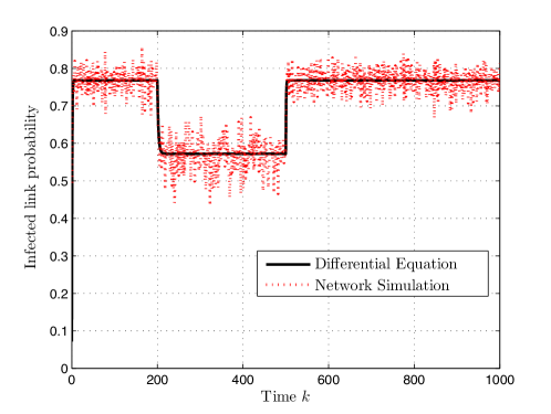
Figure 3: The infected link probability obtained from network simulation compared to the one obtained from the mean field dynamics model (12). The transition probabilities in (14) depend only on the number of infected neighbors $A^{({m})}_{k}$ (the parameters are defined in Scenario 1).

2.4 Example: Social Sensing of Influenza using Twitter

In this section, we utilize datasets from 3 different social networks (namely, (i) Harvard college social network, (ii) influenza datasets from the U.S Centers for Disease Control and Prevention (CDC) and (iii) Twitter, to show how Twitter can be used as a real time social sensor for detecting outbreaks of influenza.

2.4.1 Twitter as a social sensor

A key advantage of using social media for rapid sensing of disease outbreaks in health networks is that it is low cost and provides rapid results compared with traditional techniques. For example, CDC must contact thousands of hospitals to query the data which causes a reporting lag of approximately one to two weeks [47]. Using real time microblogging platforms such as Twitter for disease detection has several advantages: the tweets are publicly available, high tweet posting frequency users often provide meta-data (i.e. city, gender, age), and Twitter contains a diverse set of users [47].

Several papers have considered using Twitter data for estimating influenza infection rates. In [165, 188] support vector regression supervised learning algorithms is used to relate the volume of Twitter posts that contain specific words (i.e. flu, swine, influenza) to the number of confirmed influenza cases in the U.S. as reported by the CDC. Multiple linear regression [46, 48], and unsupervised Bayesian algorithms [124] have been used to relate the number of tweets of specific words to the influenza rate reported by the CDC. The detection algorithms [165, 46, 124] do not consider the dynamics of the disease propagation and the dynamics of information diffusion in the Twitter network. To reduce the effect of information diffusion in the network, [32] proposes a support vector machine (SVM) classifier to detect: a) if the tweet indicates the users awareness of influenza or indicates the user is infected, and b) if the influenza reference is in reference to another person. The classified tweets are then used to train a multiple linear regression model. To account for the diffusion dynamics of Twitter [4, 3] utilize an Autoregressive with Exogenous input (ARX) model. The exogenous input is the number of unique Twitter users with influenza related tweets, and the output is the number of infected users as reported by the CDC.

If the social network is known then the influenza spread can be formulated in terms of the diffusion model (11). Given the U.S. population of several hundred millions, it is reasonable to adopt the mean field dynamics (12). With the influenza infection rate modelled using (12), the results can be used as an exogenous input to an ARX or Nonlinear ARX (NARX) models to predict the volume of Twitter messages related to influenza as illustrated in Fig.2. In this framework, the Twitter messages are used to validate the underlying propagation model of influenza of use for predicting the infection rate and outbreak detection.

2.4.2 Social Network Influenza Dataset

We consider the dataset [43] obtained from a social network of 744 undergraduate students from Harvard College. The health of the 744 students was monitored from September 1, 2009 to December 31, 2009 and was reported by the university Health Services. To construct the social network, students were presented with a background questionnaire. In the questionnaire students are asked: “Please provide the contact information for 2-3 Harvard College students who you know and who you think would like to participate in this study”, and “…provide us with the names and contact information of 2-3 of your friends…”. This information was used to construct the degree distribution and links of the social network. A movie containing the spread of the influenza in the 744 college students over the 122 day sampling period can be viewed as the Youtube video titled “Social Network Sensors for Early Detection of Contagious Outbreaks" at http://www.youtube.com/watch?v=0TD06g2m8qM. Fig.4(a-c) display 3 illustrative snapshots from this video; red nodes denote infected students while yellow nodes depict their neighbors in the social network.

2.4.3 Models for Influenza Diffusion

From the data in the youtube video for the Harvard students, we observed the following regarding the transition probabilities $p_{ij}(d,A,s)$ defined in (5). As expected, students with a larger number of infected neighbors $A$ contract influenza sooner. The data shows that the transition probabilities were approximately independent of the degree of the node $d$. Since the data provided was during an actual influenza outbreak we set the target state of the network (i.e. ${s}$) constant. Therefore the transition probabilities depend only on the number of infected neighbours and were estimated as

$${p}_{01}(a=1)=0.02,\;{p}_{01}(a=2)=0.15.$$

That is, the dataset reveals that the probability of getting infected given $a=2$ infected neighbors is substantially higher than with $a=1$ infected neighbor, as expected. The estimated infected link probability $\theta_{k}$ in (9) versus time (days) $k$ is displayed in Fig.4(d). Recall from Sec.2.3 that the infected link probability $\theta_{k}$ is related to the mean field dynamics equation (12). This allows the transition probabilities and $\theta_{k}$ to be used to predict the infection rate dynamics.

Other graph-theoretic measures also play a role in the analysis of the diffusion. Students with high $k$-coreness are expected to contract influenza earlier. Additionally, students that have high betweenness centrality (i.e. number of shortest paths from all students to all others that pass through that student) contract influenza earlier then students with low betweenness centrality. These observations show that the diffusion of influenza in the network depends strongly on the underlying health network structure. The dynamic model (7) accounts for the effects of the degree of nodes, however to account for the effects from betweenness centrality and $k$-coreness would require a more sophisticated formulation then that presented in Sec.2.1.

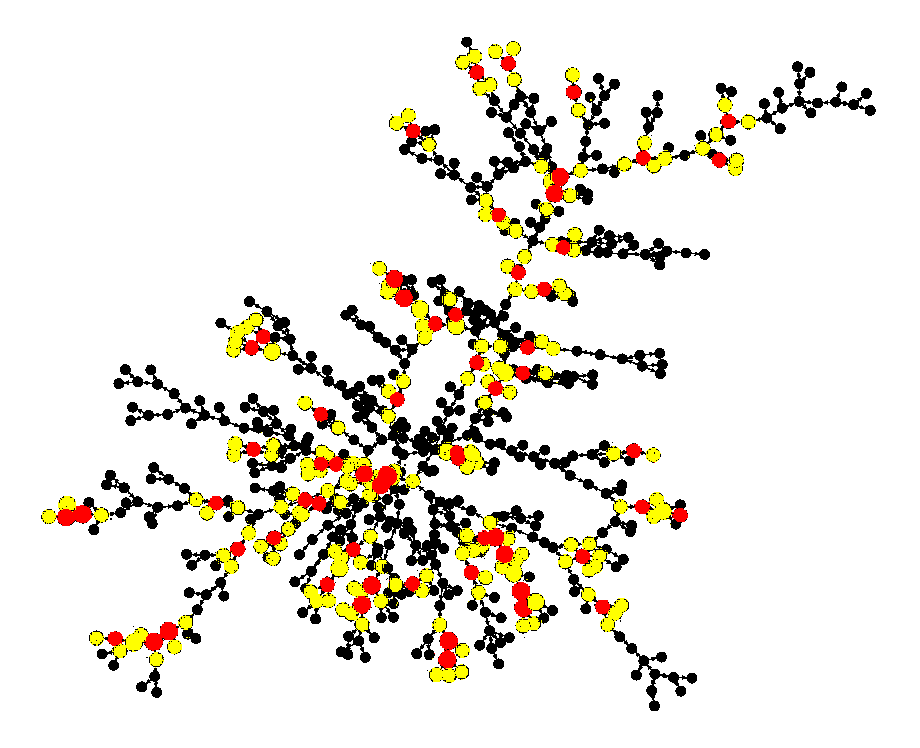
(a) October 10, 2009

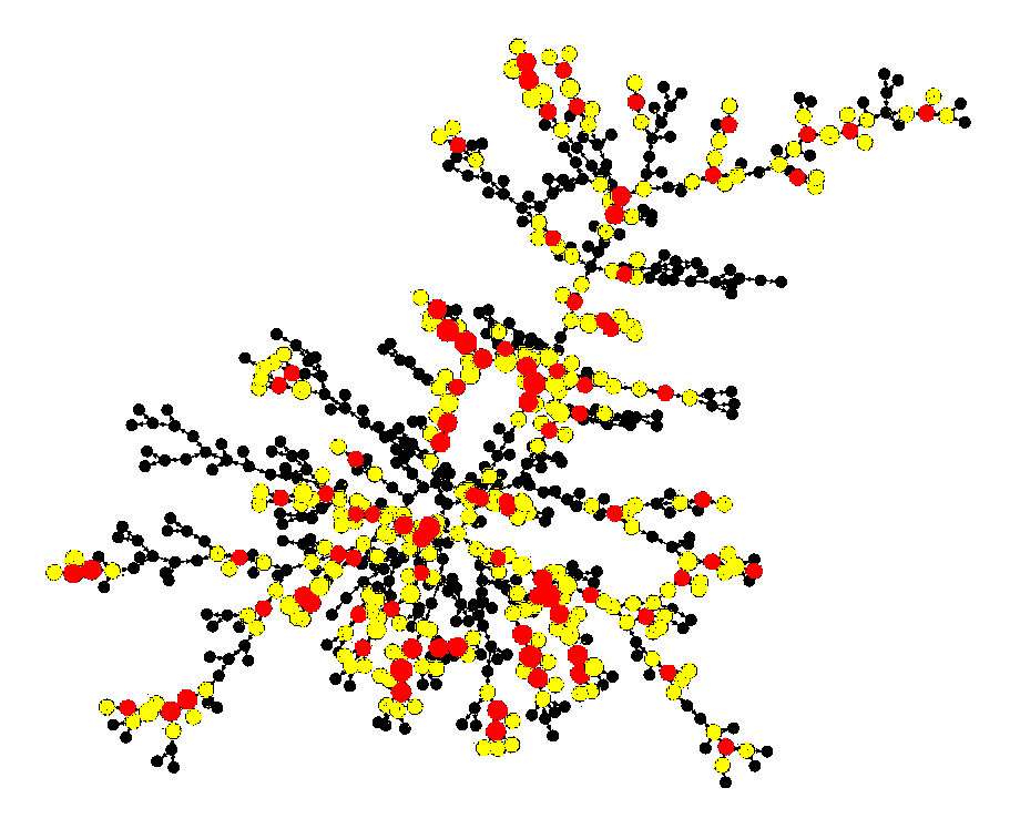
(b) November 11, 2009

(c) December 23, 2009

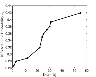
(d) Oct. 10 to Dec. 23, 2009

Figure 4: Snapshots from youtube video of Harvard undergraduate social network propagation of influenza and the estimated infected link probability $\theta_{k}$ (9) for October 10 to December 23, 2009.

2.4.4 Time series model for Influenza Tweets

In Sec.2.4.3 we illustrated how the mean field dynamics model (12) can be used to estimate the influenza infection rate with the model parameters estimated from a sampled set of the entire population. To validate the estimated parameters for the entire network requires that the infection rate be related to an observable response, in this case the number of Twitter mentions of a specific keyword. Two time series models are considered for relating the infection rate to the number of Twitter mentions. The models are validated using two real-world datasets of Twitter mentions and number of influenza cases in the U.S..

The number of influenza cases in the U.S. is obtained from the CDC which publishes weekly reports from the U.S. outpatient Influenza-like Illness Surveillance Network (ILInet). The data reported by the CDC is comprised of reports from over 3000 health providers nationwide and was obtained for the dates between September 1, 2012 to October 1, 2013. The associated Twitter data for the 122 day period was obtained using the software PeopleBrowsr. The pre-specified Twitter search terms used are: flu, swine and influenza. Since our focus is on monitoring influenza dynamics in the U.S., we excluded all tweets as tagged as originating from outside the U.S. The total number of mentions of a specific keyword on each is obtained using PeopleBrowsr.

We used two time series models for the volume of tweets and compared their performance. The first time series model considered is the ARX model defined by:

$$\tau_{k}=\sum_{i=1}^{n_{a}}a_{i}\tau_{k-i}+\sum_{i=0}^{n_{b}-1}b_{i}\rho_{k-\Delta-i}+d+v_{k}.$$ (15)

In (15), $\tau_{k}$ is the number of influenza related tweets at $k$, $\rho_{k}$ is the exogenous input of the infected influenza patients, $n_{a},n_{b},a_{i},b_{i},\Delta$ and $d$ are model parameters with $v_{k}$ an iid noise process. $\Delta$ models the delay between patient contraction, and the respective individual tweeting their symptoms. $d$ models the mean number of tweets related to influenza that are not related to an actual infection.

The second time series model we used is the nonlinear autoregressive exogenous (NARX) model given by:

$$\tau_{k}=F(\tau_{k-1},\dots,\tau_{k-n_{a}},\rho_{k-\Delta},\dots,\rho_{k-\Delta-n_{b}})+v_{k}.$$ (16)

In (16) $F$ denotes a nonlinear function which relates the exogenous input and previous tweets to the current number of tweets. Here we consider $F$ as a support vector machine which can be trained using historical data. Note that if $F$ was independent of previous tweets, previous exogenous inputs, and no delay (i.e. $n_{b}=0$ and $\Delta=0$), then (16) would be identical to the SVM classifier used in [165, 188] to relate the number of tweets to number of infected agents.

The number of reported influenza cases, associated Twitter data, and results of the model training and prediction are displayed in Fig.5 for the ARX (15) and NARX (16) models. As seen from Fig.5(a) ,the dominant word for indicating a possible influenza outbreak is flu as compared with swine and influenza. Notice that there is a lag between the maximum confirmed influenza cases and the # of tweets; however, there is an increase in the number of tweets prior to the peak of infected patients. These dynamics are a result of a combination of infection propagation dynamics and the diffusion of information on Twitter. To account for these dynamics the ARX and NARX models presented in Sec.2.4.4 are utilized. The training and prediction accuracy of these models for $n_{a}=0,n_{b}=2$ (i.e model input parameters $\rho_{k-\Delta}$ and $\rho_{k-\Delta-1}$) are displayed in Fig.5(b). As seen, the NARX (16) model provides a superior estimate as compared with the ARX model (15). Interestingly there is a $\Delta=18$ day delay between the maximum number of infected patients and the maximum number of Twitter mentions containing the word flu. This is contrast to the dynamics observed for the 2009 [165] and 2010-2011 [3] influenza outbreaks which show that the increase in Twitter mentions occurs earlier or at the same time as the number of infected patients increases. This also emphasizes the importance of using the mean field dynamics model for influenza propagation as compared with only using Twitter data for predicting the influenza infection rate. Here we have used the CDC data to estimate the number of infected agents, however the mean field dynamics model (12) could be used to estimate the dynamics of disease propagation and relate this to the observable number of tweets in real-time.

To summarize, the above datasets illustrate how Twitter can be used as a sensor for monitoring the spread of influenza in a heath network. The propagation of influenza was modeled according to the SIS model and the dynamics of tweets according to an autoregressive model.

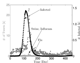
(a) Experimental data of # of tweets and # of Infected with influenza.

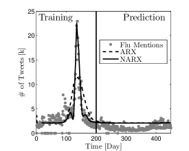
(b) ARX model (15) and NARX model (16) for the # of tweets given the # of infected influenza patients. The ARX and NARX models are trained using the initial 200 days of data. The predictive accuracy of the models is illustrated for the remaining 230 days.

Figure 5: The experimental data is obtained for September 2012 to October 2013 as described in Sec.2.4.2. The ARX (15) and NARX (16) models are utilized to estimate the number of tweets with flu given the number of infected influenza patients.

2.5 Sentiment-Based Sensing Mechanism

In the above dataset, samples of influenza affected individuals were obtained from a Harvard college social network. More generally, it is often necessary to sample individuals in a social network to estimate an underlying state of nature such as the sentiment. An important question regarding sensing in a social network is: How can one construct a small but representative sample of a social network with a large number of nodes? In [123] several scale-down and back-in-time sampling procedures are studied. Below we review three sampling schemes. The simplest possible sampling scheme is uniform sampling. We also briefly describe social sampling and respondent-driven sampling which are recent methods that have become increasingly popular.

2.5.1 Uniform Sampling

Consider the following sampling-based measurement strategy. At each period $k$, ${\alpha{(d)}}$ individuals are sampled independently and uniformly from the population ${N{(d)}}$ comprising of agents with connectivity degree $d$. That is, a uniform distributed i.i.d. sequence of nodes, denoted by$\{{m_{l}},l=1:{\alpha{(d)}}\}$, is generated from the population ${N{(d)}}$. The messages $y_{k}^{({m_{l}})}$ of these ${\alpha{(d)}}$ individuals are recorded. From these independent samples, the empirical sentiment distribution ${z}_{k}{(d)}$ of degree $d$ nodes at each time $k$ is obtained as

$${z}_{k}(d,y)=\frac{1}{{\alpha{(d)}}}\sum_{l=1}^{{\alpha{(d)}}}I\left\{y_{k}^{({m_{l}})}=y\right\},\quad y=1,\ldots,Y.$$ (17)

At each time $k$, the empirical sentiment distribution ${z}_{k}$ can be viewed as noisy observations of the infected distribution $\rho_{k}$ and target state process ${s_{k}}$.

2.5.2 Social Sampling

Social sampling is an extensive area of research; see [49] for recent results. In social sampling, participants in a poll respond with a summary of their friend’s responses. This leads to a reduction in the number of samples required. If the average degree of nodes in the network is $d$, then the savings in the number of samples is by a factor of $d$, since a randomly chosen node summarizes the results form $d$ of its friends. However, the variance and bias of the estimate depend strongly on the social network structure. In [49], a social sampling method is introduced and analyzed where nodes of degree $d$ are sampled with probability proportional to $1/d$. This is intuitive since weighing neighbors’ values by the reciprocal of the degree undoes the bias introduced by large degree nodes. It then illustrates this social sampling method and variants on the LiveJournal network (livejournal.com) comprising of more than 5 million nodes and 160 million directed edges.

2.5.3 MCMC Based Respondent-Driven Sampling (RDS)

Respondent-driven sampling (RDS) was introduced by Heckathorn [82, 83, 120] as an approach for sampling from hidden populations in social networks and has gained enormous popularity in recent years. There are more than 120 RDS studies worldwide involving sex workers and injection drug users [132]. As mentioned in [69], the U.S. Centers for Disease Control and Prevention (CDC) recently selected RDS for a 25-city study of injection drug users that is part of the National HIV Behavioral Surveillance System [117].

RDS is a variant of the well known method of snowball sampling where current sample members recruit future sample members. The RDS procedure is as follows: A small number of people in the target population serve as seeds. After participating in the study, the seeds recruit other people they know through the social network in the target population. The sampling continues according to this procedure with current sample members recruiting the next wave of sample members until the desired sampling size is reached. Typically, monetary compensations are provided for participating in the data collection and recruitment.

RDS can be viewed as a form of Markov Chain Monte Carlo (MCMC) sampling (see [69] for an excellent exposition). Let $\{{m_{l}},l=1:{\alpha{(d)}}\}$ be the realization of an aperiodic irreducible Markov chain with state space ${N{(d)}}$ comprising of nodes of degree $d$. This Markov chain models the individuals of degree $d$ that are snowball sampled, namely, the first individual ${m_{1}}$ is sampled and then recruits the second individual ${m_{2}}$ to be sampled, who then recruits ${m_{3}}$ and so on. Instead of the independent sample estimator (17), an asymptotically unbiased MCMC estimate is then generated as

$$\frac{\sum_{l=1}^{{\alpha{(d)}}}\frac{I(y_{k}^{({m_{l}})}=y)}{{\pi{({m_{l}})}}}}{\sum_{l=1}^{{\alpha{(d)}}}\frac{1}{{\pi{({m_{l}})}}}}$$ (18)

where ${\pi}({m})$, ${m}\in{N{(d)}}$, denotes the stationary distribution of the Markov chain. For example, a reversible Markov chain with prescribed stationary distribution is straightforwardly generated by the Metropolis Hastings algorithm.

In RDS, the transition matrix and, hence, the stationary distribution ${\pi}$ in the estimator (18) is specified as follows: Assume that edges between any two nodes ${m}$ and $n$ have symmetric weights $W{({m},n)}$ (i.e., $W{({m},n)}=W{(n,{m})}$, equivalently, the network is undirected). In RDS, node ${m}$ recruits node $n$ with transition probability $W{({m},n)}/\sum_{n}W{({m},n)}$. Then, it can be easily seen that the stationary distribution is $\pi({m})=\sum_{n\in V}W{({m},n)}/\sum_{{m}\in V,n\in V}W{({m},n)}$. Using this stationary distribution, along with the above transition probabilities for sampling agents in (18), yields the RDS algorithm.

It is well known that a Markov chain over a non-bipartite connected undirected network $G$ is aperiodic. Then, the initial seed for the RDS algorithm can be picked arbitrarily, and the above estimator is an asymptotically unbiased estimator.

Note the difference between RDS and social sampling: RDS uses the network to recruit the next respondent, whereas social sampling seeks to reduce the number of samples by using people’s knowledge of their friends’ (neighbors’) opinions.

Finally, the reader may be familiar with the DARPA network challenge in 2009 where the locations of 10 red balloons in the continental US were to be determined using social networking. In this case, the winning MIT Red Balloon Challenge Team used a recruitment based sampling method. The strategy can also be viewed as a variant of the Query Incentive Network model of [101].

2.6 Summary and Extensions

This section has discussed the diffusion of information in social networks. Mean field dynamics were used to approximate the asymptotic infected degree distribution. An illustrative example of the spread of influenza was provided. Finally, methods for sampling the population in a social networks were reviews. Below we discuss some related concepts and extensions.

Bayesian Filtering Problem

Given the sentiment observations described above, how can the infected degree distribution $\rho_{k}$ and target state ${s}_{k}$ be estimated at each time instant? The partially observed state space model with dynamics (12) and discrete time observations from sampling the network can be use to obtain Bayesian filtering estimates of the underlying state of nature. Computing the conditional mean estimate ${s_{k}},\rho_{k}$ given the sentiment observation sequence is a Bayesian filtering problem. In fact, filtering of such jump Markov linear systems have been studied extensively in the signal processing literature [56, 128] and can be solved via the use of sequential Markov chain Monte-Carlo methods. For example, [162] reports on how a particle filter is used to localize earthquake events using Twitter as a social sensor.

Reactive Information Diffusion

A key difference between social sensors and conventional sensors in statistical signal processing is that social sensors are reactive: A social sensor uses additional information gained to modify its behavior. Consider the case where the sentiment-based observation process is made available in a public blog. Then, these observations will affect the transition dynamics of the agents and, therefore, the mean field dynamics.

How Does Connectivity Affect Mean Field Equilibrium?

The papers [129, 130] examine the structure of fixed points of the mean field differential equation (12) when the underlying target process ${s}$ is not present (equivalently, ${s}$ is a one state process). They consider the case where the agent transition probabilities are parametrized by ${p}_{01}(d,a)=\mu F(d,a)$ and ${p}_{10}=p_{F}$. Then, defining $\lambda=\mu/p_{F}$, they study how the following two thresholds behave with the degree distribution and diffusion mechanism:

1. Critical threshold $\lambda_{c}$: This is defined as the minimum value of $\lambda$ for which there exists a fixed point of (12) with positive fraction of infected agents, i.e., $\rho_{\infty}(d)>0$ for some $d$ and, for $\lambda\leq\lambda_{c}$, such a fixed point does not exist.

2. Diffusion threshold $\lambda_{d}$: Suppose the initial condition $\rho_{0}$ for the infected distribution is infinitesimally small. Then, $\lambda_{d}$ is the minimum value of $\lambda$ for which $\rho_{\infty}(d)>0$ for some $d$, and such that, for $\lambda\leq\lambda_{d}$, $\rho_{\infty}(d)=0$ for all $d$.

Determining how these thresholds vary with degree distribution and diffusion mechanism is very useful for understanding the long term behavior of agents in the social network.

3 Bayesian Social Learning Models for Online Reputation Systems

In this section we address the second topic of the chapter, namely, Bayesian social learning amongst social sensors. The motivation can be understood in terms of the following social sensing example. Consider the following interactions in a multi-agent social network where agents seek to estimate an underlying state of nature. Each agent visits a restaurant based on reviews on an online reputation website. The agent then obtains a private measurement of the state (e.g., the quality of food in a restaurant) in noise. After that, he reviews the restaurant on the same online reputation website. The information exchange in the social network is modelled by a directed graph. Data incest [110] arises due to loops in the information exchange graph. This is illustrated in the graph of Fig.6. Agents 1 and 2 exchange beliefs (or actions) as depicted in Fig.6. The fact that there are two distinct paths between Agent 1 at time 1 and Agent 1 at time 3 (these paths are denoted in red) implies that the information of Agent 1 at time 1 is double counted leading to a data incest event.

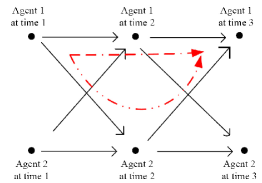
Figure 6: Example of the information flow (communication graph) in a social network with two agents and over three event epochs. The arrows represent exchange of information.

How can data incest be removed so that agents obtain a fair (unbiased) estimate of the underlying state? The methodology of this section can be interpreted in terms of the recent Time article [173] which provides interesting rules for online reputation systems. These include: (i) review the reviewers, and (ii) censor fake (malicious) reviewers. The data incest removal algorithm proposed in this chapter can be viewed as “reviewing the reviews" of other agents to see if they are associated with data incest or not.

The rest of this section is organized as follows:

1. Sec.3.1 describes the social learning model that is used to mimic the behavior of agents in online reputation systems. Sec.3.2 describes how risk averse social learning models apply to detecting market shocks in high frequency financial systems.

2. Sec.3.3 to Sec.3.5 deal with modelling data incest and incest removal algorithms for online reputation systems. The information exchange between agents in the social network is formulated on a family of time dependent directed acyclic graphs. achieves a fair rating. A necessary and sufficient condition is given on the graph structure of information exchange between agents so that a fair rating is achievable.

3. Sec.3.6 discusses conditions under which treating individual social sensors as Bayesian optimizers is a useful idealization of their behavior. In particular, it is shown that the ordinal behavior of humans can be mimicked by Bayesian optimizers under reasonable conditions.

4. Sec.3.7 presents a dataset obtained from a psychology experiment to illustrate social learning and data incest patterns.

Related work

Collaborative recommendation systems are reviewed and studied in [6, 102]. The books [36, 57] study information cascades in social learning. In [96], a model of Bayesian social learning is considered in which agents receive private information about the state of nature and observe actions of their neighbors in a tree-based network. Another type of mis-information caused by influential agents (agents who heavily affect actions of other agents in social networks) is investigated in [2]. Mis-information in the context of this chapter is motivated by sensor networks where the term “data incest" is used [110]. Data incest also arises in Belief Propagation (BP) algorithms [152, 140] which are used in computer vision and error-correcting coding theory. BP algorithms require passing local messages over the graph (Bayesian network) at each iteration. For graphical models with loops, BP algorithms are only approximate due to the over-counting of local messages [185] which is similar to data incest in social learning. With the algorithms presented in this section, data incest can be mitigated from Bayesian social learning over non-tree graphs that satisfy a topological constraint. The closest work to the current chapter is [110]. However, in [110], data incest is considered in a network where agents exchange their private belief states - that is, no social learning is considered. Simpler versions of this information exchange process and estimation were investigated in [16, 65, 29]. We also refer the reader to [40] for a discussion of recommender systems.

3.1 Classical Social Learning

We briefly review the classical social learning model for the interaction of individuals. Subsequently, we will deal with more general models over a social network.

Consider a multi-agent system that aims to estimate the state of an underlying finite state random variable $x\in\mathbb{X}=\{1,2,\ldots,X\}$ with known prior distribution $\pi_{0}$. Each agent acts once in a predetermined sequential order indexed by $k=1,2,\ldots$ Assume at the beginning of iteration $k$, all agents have access to the public belief $\pi_{k-1}$ defined in Step (iv) below. The social learning protocol proceeds as follows [25, 36]:
(i) Private Observation: At time $k$, agent $k$ records a private observation $y_{k}\in\mathbb{Y}$ from the observation distribution $B_{iy}=P(y|x=i)$, $i\in\mathbb{X}$. Throughout this section we assume that $\mathbb{Y}=\{1,2,\ldots,Y\}$ is finite.
(ii) Private Belief: Using the public belief $\pi_{k-1}$ available at time $k-1$ (Step (iv) below), agent $k$ updates its private posterior belief $\eta_{k}(i)=P(x_{k}=i|a_{1},\ldots,a_{k-1},y_{k})$ using Bayes formula:

$$\eta_{k} =\frac{B_{y_{k}}\pi}{\mathbf{1}_{X}^{\prime}B_{y}\pi},\;B_{y_{k}}=\text{diag}(P(y_{k}|x=i),i\in\mathbb{X}).$$ (19)

Here $\mathbf{1}_{X}$ denotes the $X$-dimensional vector of ones, $\eta_{k}$ is an $X$-dimensional probability mass function (pmf).
(iii) Myopic Action: Agent $k$ takes action $a_{k}\in\mathcal{A}=\{1,2,\ldots,A\}$ to minimize its expected cost

$$a_{k}=\arg\min_{a\in\mathcal{A}}\mathbf{E}\{c(x,a)|a_{1},\ldots,a_{k-1},y_{k}\}=\arg\min_{a\in\mathcal{A}}\{c_{a}^{\prime}\eta_{k}\}.$$ (20)

Here $c_{a}=(c(i,a),i\in\mathbb{X})$ denotes an $X$ dimensional cost vector, and $c(i,a)$ denotes the cost incurred when the underlying state is $i$ and the agent chooses action $a$.
Agent $k$ then broadcasts its action $a_{k}$.
(iv) Social Learning Filter: Given the action $a_{k}$ of agent $k$, and the public belief $\pi_{k-1}$, each subsequent agent $k^{\prime}>k$ performs social learning to update the public belief $\pi_{k}$ according to the “social learning filter":

$$\pi_{k}=T(\pi_{k-1},a_{k}),\text{ where }T(\pi,a)=\frac{R^{\pi}_{a}\,\pi}{\sigma(\pi,a)},$$ (21)

where $\sigma(\pi,a)=\mathbf{1}_{X}^{\prime}R^{\pi}_{a}P^{\prime}\pi$ is the normalization factor of the Bayesian update. In (21), the public belief $\pi_{k}(i)=P(x_{k}=i|a_{1},\ldots a_{k})$ and $R^{\pi}_{a}=\text{diag}(P(a|x=i,\pi),i\in\mathbb{X})$ has elements

$$P(a_{k}=a|x_{k}=i,\pi_{k-1}=\pi)=\sum_{y\in\mathbb{Y}}P(a|y,\pi)P(y|x_{k}=i)$$

$$P(a_{k}=a|y,\pi)=\begin{cases}1\text{ if }c_{a}^{\prime}B_{y}P^{\prime}\pi\leq c_{\tilde{a}}^{\prime}B_{y}P^{\prime}\pi,\;\tilde{a}\in\mathcal{A}\\ 0\text{ otherwise. }\end{cases}$$

The following result which is well known in the economics literature [25, 36] states that if agents follow the above social learning protocol, then after some finite time $\bar{k}$, an information cascade occurs.

Theorem 3.1 ([25]).

The social learning protocol leads to an information cascade in finite time with probability 1. That is, after some finite time $\bar{k}$ social learning ceases and the public belief $\pi_{k+1}=\pi_{k}$, $k\geq\bar{k}$, and all agents choose the same action $a_{k+1}=a_{k}$, $k\geq\bar{k}$. ∎

Instead of reproducing the proof, let us give some insight as to why Theorem 3.1 holds. It can be shown using martingale methods that at some finite time $k=k^{*}$, the agent’s probability $P(a_{k}|y_{k},\pi_{k-1})$ becomes independent of the private observation $y_{k}$. Then clearly, $P(a_{k}=a|x_{k}=i,\pi_{k-1})=P(a_{k}=a|\pi)$. Substituting this into the social learning filter (21), we see that $\pi_{k}=\pi_{k-1}$. Thus after some finite time $k^{*}$, the social learning filter hits a fixed point and social learning stops. As a result, all subsequent agents $k>k^{*}$ completely disregard their private observations and take the same action $a_{k^{*}}$, thereby forming an information cascade (and therefore a herd).

3.2 Risk Averse Social Learning and Detecting Market Shocks

Here we consider the statistical signal processing problem involving agent based models of financial markets which at a micro-level are driven by socially aware and risk-averse trading agents. These agents trade (buy or sell) stocks at each trading instant by using the decisions of all previous agents (social learning) in addition to a private (noisy) signal they receive on the value of the stock. We are interested in the following: (1) Modelling the dynamics of these risk averse agents, (2) Sequential detection of a market shock based on the behaviour of these agents. Structural results which characterize social learning under a risk measure, CVaR (Conditional Value-at-risk), are presented and formulation of the Bayesian change point detection problem is provided. The structural results exhibit two interesting properties: (i) Risk averse agents herd more often than risk neutral agents (ii) The stopping set in the sequential detection problem is non-convex.

It is well documented in behavioural economics [44] and psychology [55] that people prefer a certain but possibly less desirable outcome over an uncertain but potentially larger outcome. To model this risk averse behaviour, commonly used risk measures are Value-at-Risk (VaR), Conditional Value-at-Risk (CVaR), Entropic risk measure and Tail value at risk; see [138]. We consider social learning under CVaR risk measure. CVaR [158] is an extension of VaR that gives the total loss given a loss event and is a coherent risk measure [14]. Below, we choose CVaR risk measure as it exhibits the following properties [14], [158]: (i) It associates higher risk with higher cost. (ii) It ensures that risk is not a function of the quantity purchased, but arises from the stock. (iii) It is convex. CVaR as a risk measure has been used in solving portfolio optimization problems [149], [125] and order execution. For an overview of risk measures and their application in finance, see [138].

CVaR Social Learning Model

The market micro-structure is modelled as a discrete time dealer market motivated by algorithmic and high-frequency tick-by-tick trading [34]. There is a single traded stock or asset, a market observer and a countable number of trading agents. The asset has an initial true underlying value $x_{0}\in\mathcal{X}=\{1,2,\ldots,X\}$. The market observer does not receive direct information about $x\in\mathcal{X}$ but only observes the public buy/sell actions of agents, $a_{k}\in\mathcal{A}=\{1(\text{buy}),2({\text{sell}})\}$. The agents themselves receive noisy private observations of the underlying value $x$ and consider this in addition to the trading decisions of the other agents visible in the order book. At a random time, $\tau^{0}$ determined by the transition matrix $P$, the asset experiences a jump change in its value to a new value. The aim of the market observer is to detect the change time (global decision) with minimal cost, having access to only the actions of these socially aware agents. Let $y_{k}\in\mathcal{Y}=\{1,2,\ldots,Y\}$ denote agent $k$’s private observation. The initial distribution is $\pi_{0}=(\pi_{0}(i),i\in\mathcal{X})$ where $\pi_{0}(i)=\mathbb{P}(x_{0}=i)$.

The agent based model has the following dynamics:

1. Shock in the asset value: At time $\tau^{0}>0$, the asset experiences a jump change (shock) in its value due to exogenous factors. The change point $\tau^{0}$ is modelled by a phase type (PH) distribution. The family of all PH-distributions forms a dense subset for the set of all distributions [144] i.e., for any given distribution function $F$ such that $F(0)=0$, one can find a sequence of PH-distributions $\{F_{n},n\geq 1\}$ to approximate $F$ uniformly over $[0,\infty)$. The PH-distributed time $\tau^{0}$ can be constructed via a multi-state Markov chain $x_{k}$ with state space $\mathcal{X}=\{1,\ldots,X\}$ as follows: Assume state ‘1’ is an absorbing state and denotes the state after the jump change. The states $2,\ldots,X$ (corresponding to beliefs $e_{2},\ldots,e_{X}$) can be viewed as a single composite state that $x$ resides in before the jump. So $\tau^{0}=\text{inf}\{{k:x_{k}=1}\}$ and the transition probability matrix $P$ is of the form

   $$P=\begin{bmatrix}1&0\\ \underline{P}_{(X-1)\times 1}&{\bar{P}_{(X-1)\times(X-1)}}\end{bmatrix}$$ (22)

   The distribution of the absorption time to state 1 is

   $$\nu_{0}=\pi_{0}(1),\quad\nu_{k}=\bar{\pi}_{0}^{\prime}\bar{P}^{k-1}\underline{P},\quad k\geq 1,$$ (23)

   where $\bar{\pi}_{0}=[\pi_{0}(2),\ldots,\pi_{0}(X)]^{\prime}$. The key idea is that by appropriately choosing the pair $(\pi_{0},P)$ and the associated state space dimension $X$, one can approximate any given discrete distribution on $[0,\infty)$ by the distribution $\{\nu_{k},k\geq 0\}$; see [144, pp.240-243]. The event $\{x_{k}=1\}$ means the change point has occurred before time $k$ according to PH-distribution (23). In the special case when $x$ is a 2-state Markov chain, the change time $\tau^{0}$ is geometrically distributed.

2. Agent’s Private Observation: Agent $k$’s private (local) observation denoted by $y_{k}$ is a noisy measurement of the true value of the asset. It is obtained from the observation likelihood distribution as,

   $$B_{xy}=\mathbb{P}(y_{k}=y|x_{k}=x)$$ (24)

3. Private Belief update: Agent $k$ updates its private belief using the observation $y_{k}$ and the prior public belief $\pi_{k-1}(i)=\mathbb{P}(X=i|a_{1},\ldots,a_{k-1})$ as the following Hidden Markov Model update

   $$\eta_{k}=\frac{B_{y_{k}}P^{\prime}\pi_{k-1}}{\textbf{1}^{\prime}B_{y_{k}}P^{\prime}\pi_{k-1}}$$ (25)

   where 1 denotes the $X$-dimensional vector of ones.

4. Agent’s trading decision: Agent $k$ executes an action $a_{k}\in\mathcal{A}=\{1(\text{buy}),2(\text{sell})\}$ to myopically minimize its cost. Let $c(i,a)$ denote the cost incurred if the agent takes action $a$ when the underlying state is $i$. Let the local cost vector be

   $$c_{a}=[c(1,a)~{}c(2,a)\dots~{}c(X,a)]$$ (26)

   The costs for different actions are taken as

   $$c(i,j)=p_{j}-\beta_{ij}~{}\text{for}~{}i\in\mathcal{X},j\in\mathcal{A}$$ (27)

   where $\beta_{ij}$ corresponds to the agent’s demand. Here demand is the agent’s desire and willingness to trade at a price $p_{j}$ for the stock. Here $p_{1}$ is the quoted price for purchase and $p_{2}$ is the price demanded in exchange for the stock. We assume that the price is the same during the period in which the value changes. As a result, the willingness of each agent only depends on the degree of uncertainty on the value of the stock.

   Remark 3.2.

   The analysis provided in this paper straightforwardly extends to the case when different agents are facing different prices like in an order book. For notational simplicity we assume the cost are time invariant.

   The agent considers measures of risk in the presence of uncertainty in order to overcome the losses incurred in trading. To illustrate this, let $c(x,a)$ denote the loss incurred with action $a$ while at unknown and random state $x\in{\mathcal{X}}$. When an agent solves an optimization problem involving $c(x,a)$ for selecting the best trading decision, it will take into account not just the expected loss, but also the “riskiness" associated with the trading decision $a$. The agent therefore chooses an action $a_{k}$ to minimize the CVaR measure of trading as

   $$a_{k} ={\underset{a\in\mathcal{A}}{\text{argmin}}}\{\text{CVaR}_{\alpha}(c(x_{k},a))\}$$ (28)

   $$={\underset{a\in\mathcal{A}}{\text{argmin}}}\{{\underset{z\in\mathbb{R}}{\text{min}}}~{}\{z+\frac{1}{\alpha}\mathbb{E}_{y_{k}}[{\max}\{(c(x_{k},a)-z),0\}]\}\}$$

   Here $\alpha\in(0,1]$ reflects the degree of risk-aversion for the agent (the smaller $\alpha$ is, the more risk-averse the agent is). Define

   $$\mathcal{H}_{k}:=\sigma\text{- algebra generated by}~{}(a_{1},a_{2},\ldots,a_{k-1},y_{k})$$ (29)

   $\mathbb{E}_{y_{k}}$ denotes the expectation with respect to private belief, i.e, $\mathbb{E}_{y_{k}}=\mathbb{E}[.|\mathcal{H}_{k}]$ when the private belief is updated after observation $y_{k}$.

5. Social Learning and Public belief update: Agent $k$’s action is recorded in the order book and hence broadcast publicly. Subsequent agents and the market observer update the public belief on the value of the stock according to the social learning Bayesian filter as follows

   $$\pi_{k}=T^{\pi_{k-1}}(\pi_{k-1},a_{k})=\frac{R_{a_{k}}^{\pi_{k-1}}P^{\prime}\pi_{k-1}}{\textbf{1}^{\prime}R_{a_{k}}^{\pi_{k-1}}P^{\prime}\pi_{k-1}}$$ (30)

   Here, $R_{a_{k}}^{\pi_{k-1}}=\text{diag}(\mathbb{P}(a_{k}|x=i,\pi_{k-1}),i\in\mathcal{X})$, where $\mathbb{P}(a_{k}|x=i,\pi_{k-1})={\underset{y\in\mathcal{Y}}{\sum}}\mathbb{P}(a_{k}|y,\pi_{k-1})\mathbb{P}(y|x_{k}=i)$ and

   $$\mathbb{P}(a_{k}|y,\pi_{k-1})=\left\{\begin{array}[]{ll}1&\mbox{if $a_{k}={\underset{a\in\mathcal{A}}{\text{argmin}}}~{}\text{CVaR}_{\zeta}(c(x_{k},a))$};\\ 0&\mbox{$\text{otherwise}$}.\end{array}\right.$$

   Note that $\pi_{k}$ belongs to the unit simplex $\Pi(X){\overset{\Delta}{=}}\{\pi\in\mathbb{R}^{X}:\textbf{1}_{X}^{\prime}\pi=1,0\leq\pi\leq 1~{}\text{for all}~{}i\in\mathcal{X}\}$.

6. Market Observer’s Action: The market observer (securities dealer) seeks to achieve quickest detection by balancing delay with false alarm. At each time $k$, the market observer chooses action $u_{k}$ as

   $$u_{k}\in\mathcal{U}=\{1(\text{stop}),2(\text{continue})\}$$ (31)

   Here ‘Stop’ indicates that the value has changed and the dealer incorporates this information before selling new issues to investors. The formulation presented considers a general parametrization of the costs associated with detection delay and false alarm costs. Define

   $$\mathcal{G}_{k}:=\sigma\text{- algebra generated by}~{}(a_{1},a_{2},\ldots,a_{k-1},a_{k}).$$ (32)

   • Cost of Stopping: The asset experiences a jump change(shock) in its value at time $\tau^{0}$. If the action $u_{k}=1$ is chosen before the change point, a false alarm penalty is incurred. This corresponds to the event ${\underset{i\geq 2}{\cup}}\{x_{k}=i\}\cap\{u_{k}=1\}$. Let $\mathcal{I}$ denote the indicator function. The cost of false alarm in state $i,i\in\mathcal{X}$ with $f_{i}\geq 0$ is thus given by $f_{i}\mathcal{I}(x_{k}=i,u_{k}=1)$. The expected false alarm penalty is

     $$C(\pi_{k},u_{k}=1) ={\underset{i\in\mathcal{X}}{\sum}}f_{i}\mathbb{E}\{\mathcal{I}(x_{k}=i,u_{k}=1)|\mathcal{G}_{k}\}$$

     $$=\textbf{f}^{\prime}\pi_{k}$$ (33)

     where $\textbf{f}=(f_{1},\ldots,f_{X})$ and it is chosen with increasing elements, so that states further from ‘$1$’ incur higher false alarm penalties. Clearly, $f_{1}=0$.

   • Cost of delay: A delay cost is incurred when the event $\{x_{k}=1,u_{k}=2\}$ occurs, i.e, even though the state changed at $k$, the market observer fails to identify the change. The expected delay cost is

     $$C(\pi_{k},u_{k}=2) =d\,\mathbb{E}\{\mathcal{I}(x_{k}=i,u_{k}=1)|\mathcal{G}_{k}\}$$

     $$=de_{1}^{\prime}\pi_{k}$$ (34)

     where $d>0$ is the delay cost and $e_{1}$ denotes the unit vector with 1 in the first position.

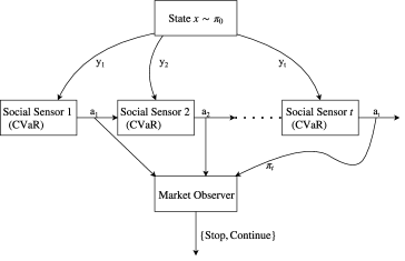
Figure 7: Sequential detection with risk-averse social sensors. Each social sensor receives a noisy observation on the state and chooses an action to minimize its CVaR measure of trading. The social sensors communicate their actions to subsequent sensors. The market observer seeks to determine if there is a change in the value of the underlying asset from the actions of the sensors.

Fig. 7 illustrates the above social learning model in which the information exchange between the risk-averse social sensors is sequential.

Market Observer’s Quickest Detection Objective

The market observer chooses its action at each time $k$ as

$$u_{k}=\mu(\pi_{k})\in\{1(\text{stop}),2(\text{continue})\}$$ (35)

where $\mu$ denotes a stationary policy. For each initial distribution $\pi_{0}\in\Pi(X)$ and policy $\mu$, the following cost is associated

$$J_{\mu}(\pi_{0})=\mathbb{E}^{\mu}_{\pi_{0}}\left\{{\overset{\tau-1}{\underset{k=1}{\sum}}}\rho^{k-1}C(\pi_{k},u_{k}=2)+\rho^{\tau-1}C(\pi_{k},u_{k}=1)\right\}$$ (36)

Here $\rho\in[0,1]$ is the discount factor which is a measure of the degree of impatience of the market observer. (As long as f is non-zero, stopping is guaranteed in finite time and so $\rho=1$ is allowed.)

Given the cost, the market observer’s objective is to determine $\tau^{0}$ with minimum cost by computing an optimal policy $\mu^{*}$ such that

$$J_{\mu^{*}}(\pi_{0})={\underset{\mu\in\boldsymbol{\mu}}{\text{inf}}J_{\mu}(\pi_{0})}$$ (37)

The sequential detection problem (37) can be viewed as a partially observed Markov decision process (POMDP) where the belief update is given by the social learning filter.

Stochastic Dynamic Programming Formulation

The optimal policy of the market observer $\mu^{*}:\Pi(X)\rightarrow\{1,2\}$ is the solution of (36) and is given by Bellman’s dynamic programming equation as follows:

$$V(\pi) =\text{min}\left\{C(\pi,1),C(\pi,2)+\rho{\underset{a\in\mathcal{A}}{\sum}}V(T^{\pi}(\pi,a))\sigma(\pi,a)\right\}$$ (38)

$$\mu^{*}(\pi) =\text{argmin}\left\{C(\pi,1),C(\pi,2)+\rho{\underset{a\in\mathcal{A}}{\sum}}V(T^{\pi}(\pi,a))\sigma(\pi,a)\right\}$$

where $T^{\pi}(\pi,a)=\frac{R_{a}^{\pi}P^{\prime}\pi}{\textbf{1}^{\prime}R_{a}^{\pi}P^{\prime}\pi}$ is the CVaR-social learning filter and $\sigma(\pi,a)=\textbf{1}^{\prime}R_{a}^{\pi}P^{\prime}\pi$ is the normalization factor of the Bayesian update. $C(\pi,1)$ and $C(\pi,2)$ from (i)) and (ii)) are the market observer’s costs. As $C(\pi,1)$ and $C(\pi,2)$ are non-negative and bounded for $\pi\in\Pi(X)$, the stopping time $\tau$ is finite for all $\rho\in[0,1]$.

The aim of the market observer is then to determine the stopping set $\mathcal{S}=\{\pi\in\Pi(X):\mu^{*}(\pi)=1\}$ given by:

$$\mathcal{S}=\left\{\pi:C(\pi,1)<C(\pi,2)+\rho{\underset{a\in\mathcal{A}}{\sum}}V(T^{\pi}(\pi,a))\sigma(\pi,a)\right\}$$

The dynamic programming equation (38) is similar to that for stopping time POMDP except that the belief update is given by a CVaR social learning filter. As will be shown below, because of the social learning dynamics, quite remarkably, $\mathcal{S}$ is not necessarily a convex set. This is in stark contrast to classical quickest detection where the stopping region is always convex irrespective of the change time distribution [104].

Social Learning Behavior of Risk Averse Agents

The following discussion highlights the relation between risk-aversion factor $\alpha$ and the regions $\mathcal{P}^{\alpha}_{l}$. For a given risk-aversion factor $\alpha$, it can be shown that there are at most $Y+1$ polytopes on the belief space. It was shown in [105] that for the risk neutral case with $X=2$, and $P=I$ (the value is a random variable) the intervals $\mathcal{P}^{\alpha}_{1}$ and $\mathcal{P}^{\alpha}_{3}$ correspond to the herding region and the interval $\mathcal{P}^{\alpha}_{2}$ corresponds to the social learning region. In the herding region, the agents take the same action as the belief is frozen. In the social learning region there is observational learning. However, when the agents are optimizing a more general risk measure (CVaR), the social learning region is different for different risk-aversion factors. The social learning region for the CVaR risk measure is shown in Fig. 8. It can be observed from Fig. 8 that $\mathcal{P}^{\alpha}_{1}$ becomes smaller, $\mathcal{P}^{\alpha}_{2}$ becomes smaller and $\mathcal{P}^{\alpha}_{3}$ becomes larger as $\alpha$ decreases.

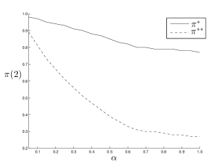
Figure 8: The social learning region for the risk-aversion parameter $\alpha\in(0,1]$. It can be seen that the curves corresponding to $\pi^{**}$ and $\pi^{*}$ do not intersect and their separation (social learning region) varies with $\alpha$. Here $P=I$, i.e, the value is a random variable.

The following parameters were chosen:

$$B=\begin{bmatrix}0.8&0.2\\ 0.3&0.7\end{bmatrix},P=\begin{bmatrix}1&0\\ 0&1\end{bmatrix},c=\begin{bmatrix}1&2\\ 3&0.5\end{bmatrix}$$

This can be interpreted as risk-averse agents showing a larger tendency to go with the crowd rather than “risk" choosing the other action. With the same $B$ and $c$ parameters, but with transition matrix

$$P=\begin{bmatrix}1&0\\ 0.1&0.9\end{bmatrix}$$

the social learning region is shown in Fig. 9.

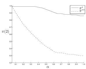
Figure 9: The social learning region for the risk-aversion parameter $\alpha\in(0,1]$. It can be seen that the social learning region is absent when agents are sufficiently risk-averse and is larger when the stock value is known to change, i.e, $P\neq I$.

From Fig. 9, it is observed that when the state is evolving and when the agents are sufficiently risk-averse, social learning region is very small. It can be interpreted as: agents having a strong risk-averse attitude don’t prefer to “learn" from the crowd; but rather face the same consequences, when $P\neq I$.

Nonconvex Stopping Set for Market Shock Detection

We now illustrate the solution to the Bellman’s stochastic dynamic programming equation (38), which determines the optimal policy for quickest market shock detection, by considering an agent based model with two states. Clearly the agents (local decision makers) and market observer interact – the local decisions $a_{k}$ taken by the agents determines the public belief $\pi_{k}$ and hence determines decision $u_{k}$ of the market observer via (35).

Fig. 10 displays the value function and optimal policy for a toy example having the following parameters:

$$B=\begin{bmatrix}0.8&0.2\\ 0.3&0.7\end{bmatrix},P=\begin{bmatrix}1&0\\ 0.06&0.94\end{bmatrix},c=\begin{bmatrix}1&2\\ 2.5&0.5\end{bmatrix}$$

The parameters for the market observer are chosen as: $d=1.25$, $\textbf{f}=[0~{}3]$, $\alpha=0.8$ and $\rho=0.9$.

From Fig. 10 it is clear that the market observer has a double threshold policy and the value function is discontinuous. The double threshold policy is unusual from a signal processing point of view. Recall that $\pi(2)$ depicts the posterior probability of no change. The market observer “changes its mind" - it switches from no change to change as the posterior probability of change decreases! Thus the global decision (stop or continue) is a non-monotone function of the posterior probability obtained from local decisions in the agent based model. The example illustrates the unusual behaviour of the social learning filter.

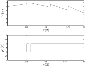
Figure 10: The value function $V(\pi)$ and the double threshold optimal policy $\mu^{*}(\pi)$ are plotted over $\pi(2)$. The significance of the double threshold policy is that the stopping regions are non-convex. The implication of non-convex stopping set for the market observer is that - if he believes that it is optimal to stop, it need not be optimal to stop when his belief is larger.

Summary

In this subsection we provided a Bayesian formulation of the problem of quickest detection of change in the value of a stock using the decisions of socially aware risk averse agents. The quickest detection problem was shown to be non-trivial - the stopping region is in general non-convex when the agents’ risk attitude was accounted for by considering a coherent risk measure, CVaR. Results which characterize the structural properties of social learning under the CVaR risk measure were provided and the importance of these results in understanding the global behaviour was discussed. It was observed that the behaviour of these risk-averse agents is, as expected, different from risk neutral agents. Risk averse agents herd sooner and do not prefer to “learn" from the crowd, i.e, social learning region is smaller the more risk-averse the agents are. For further structural results on the risk averse social learning filter, please see [107].

3.3 Data Incest in Online Reputation Systems

In comparison to the previous subsections , where social learning model was formulated on a line graph, we now consider social learning on a family of time dependent directed acyclic graphs - in such cases, apart from herding, the phenomenon of data incest arises.

Consider an online reputation system comprised of agents $\{1,2,\ldots,S\}$ that aim to estimate an underlying state of nature (a random variable). Let $x\in\mathbb{X}=\{1,2,\ldots,X\}$ represent the state of nature (such as the quality of a restaurant/hotel) with known prior distribution $\pi_{0}$. Let $k=1,2,3,\ldots$ depict epochs at which events occur. These events involve taking observations, evaluating beliefs and choosing actions as described below. The index $k$ marks the historical order of events. For simplicity, we refer to $k$ as “time".

It is convenient also to reduce the coordinates of time $k$ and agent $s$ to a single integer index $n$:

$$n\triangleq s+S(k-1),\quad s\in\{1,\ldots,S\},\;k=1,2,3,\ldots$$ (39)

We refer to $n$ as a “node" of a time dependent information flow graph $G_{n}$ which we now define. Let

$$G_{n}=(V_{n},E_{n}),\quad n=1,2,\ldots$$ (40)

denote a sequence of time-dependent directed acyclic graphs (DAGs) of information flow in the social network until and including time $k$ where $n=s+S(k-1)$. Each vertex in $V_{n}$ represents an agent $s^{\prime}$ in the social network at time $k^{\prime}$ and each edge $(n^{\prime},n^{\prime\prime})$ in $E_{n}\subseteq V_{n}\times V_{n}$ shows that the information (action) of node $n^{\prime}$ (agent $s^{\prime}$ at time $k^{\prime}$) reaches node $n^{\prime\prime}$ (agent $s^{\prime\prime}$ at time $k^{\prime\prime}$). It is clear that $G_{n}$ is a sub-graph of $G_{n+1}$.

The Adjacency Matrix $A_{n}$ of $G_{n}$ is an $n\times n$ matrix with elements $A_{n}(i,j)$ given by

$$A_{n}(i,j)=\begin{cases}1&\textrm{ if }(v_{j},v_{i})\in E\;,\\ 0&\textrm{ otherwise}\end{cases}\;,\text{ }A_{n}(i,i)=0.$$ (41)

The transitive closure matrix $T_{n}$ is the $n\times n$ matrix

$$T_{n}=\text{sgn}((\mathbf{I}_{n}-A_{n})^{-1})$$ (42)

where for matrix $M$, the matrix $\text{sgn}(M)$ has elements

$$\text{sgn}(M)(i,j)=\begin{cases}0&\text{ if }M(i,j)=0\;,\\ 1&\text{ if }M(i,j)\neq 0.\end{cases}$$

Note that $A_{n}(i,j)=1$ if there is a single hop path between nodes $i$ and $j$, In comparison, $T_{n}(i,j)=1$ if there exists a path (possible multi-hop) between $i$ and $j$.

The information reaching node $n$ depends on the information flow graph $G_{n}$. The following two sets will be used to specify the incest removal algorithms below:

$$\mathcal{H}_{n} =\{m:A_{n}(m,n)=1\}$$ (43)

$$\mathcal{F}_{n} =\{m:T_{n}(m,n)=1\}.$$ (44)

Thus $\mathcal{H}_{n}$ denotes the set of previous nodes $m$ that communicate with node $n$ in a single-hop. In comparison, $\mathcal{F}_{n}$ denotes the set of previous nodes $m$ whose information eventually arrives at node $n$. Thus $\mathcal{F}_{n}$ contains all possible multi-hop connections by which information from a node $m$ eventually reaches node $n$.

Example

Consider $S=2$ two agents with information flow graph for three time points $k=1,2,3$ depicted in Fig.11 characterized by the family of DAGs $\{G_{1},\ldots,G_{7}\}$. The adjacency matrices $A_{1},\ldots,A_{7}$ are constructed as follows: $A_{n}$ is the upper left $n\times n$ submatrix of $A_{n+1}$ and

$${\small A_{7}=\begin{bmatrix}0&0&1&1&0&0&1\\ 0&0&0&1&0&0&0\\ 0&0&0&0&1&0&0\\ 0&0&0&0&0&1&0\\ 0&0&0&0&0&0&1\\ 0&0&0&0&0&0&1\\ 0&0&0&0&0&0&0\\ \end{bmatrix}}.$$

Figure 11: Example of information flow network with $S=2$ two agents, namely $s\in\{1,2\}$ and time points $k=1,2,3,4$. Circles represent the nodes indexed by $n=s+S(k-1)$ in the social network and each edge depicts a communication link between two nodes.

Let us explain these matrices. Since nodes 1 and 2 do not communicate, clearly $A_{1}$ and $A_{2}$ are zero matrices. Nodes 1 and 3 communicate, hence $A_{3}$ has a single one, etc. Note that if nodes 1,3,4 and 7 are assumed to be the same individual, then at node 7, the individual remembers what happened at node 5 and node 1, but not node 3. This models the case where the individual has selective memory and remembers certain highlights. From (43) and (44),

$$\mathcal{H}_{7}=\{1,5,6\},\quad\mathcal{F}_{7}=\{1,2,3,4,5,6\}$$

where $\mathcal{H}_{7}$ denotes all one hop links to node 7 while $\mathcal{F}_{7}$ denotes all multihop links to node 7.

3.4 Data Incest Model and Social Influence Constraint

Each node $n$ receives recommendations from its immediate friends (one hop neighbors) according to the information flow graph defined above. That is, it receives actions $\{a_{m},m\in\mathcal{H}_{n}\}$ from nodes $m\in\mathcal{H}_{n}$ and then seeks to compute the associated public beliefs ${\pi}_{m},m\in\mathcal{H}_{n}$. If node $n$ naively (incorrectly) assumes that the public beliefs ${\pi}_{m},m\in\mathcal{H}_{n}$ are independent, then it would fuse these as

$${\pi}_{n}{-}=\frac{\prod_{m\in\mathcal{H}_{n}}{\pi}_{m}}{\mathbf{1}_{X}^{\prime}\prod_{m\in\mathcal{H}_{n}}{\pi}_{m}}.\text{ (WRONG!)}$$ (45)

This naive data fusion would result in data incest.

3.4.1 Aim

The aim is to provide each node $n$ the true posterior distribution

$$\pi^{0}_{n-}(i)=P(x=i|\{a_{m},m\in\mathcal{F}_{n}\})$$ (46)

subject to the following social influence constraint: There exists a fusion algorithm $\mathcal{A}$ such that

$$\pi^{0}_{n-}=\mathcal{A}(\pi_{m},m\in\mathcal{H}_{n}).$$ (47)

3.4.2 Discussion. Fair Rating and Social Influence

We briefly pause to discuss (46) and (47).
(i) We call $\pi^{0}_{n-}$ in (46) the true or fair online rating available to node $n$ since $\mathcal{F}_{n}$ defined in (44) denotes all information (multi-hop links) available to node $n$. By definition $\pi^{0}_{n-}$ is incest free and is the desired conditional probability that agent $n$ needs.

Indeed, if node $n$ combines $\pi^{0}_{n-}$ together with its own private observation via social learning, then clearly

$$\eta_{n}(i) =P(x=i|\{a_{m},m\in\mathcal{F}_{n}\},y_{n}),\quad i\in\mathbb{X},$$

$$\pi_{n}(i) =P(x=i|\{a_{m},m\in\mathcal{F}_{n}\},a_{n}),\quad i\in\mathbb{X},$$

are, respectively, the correct (incest free) private belief for node $n$ and the correct after-action public belief. If agent $n$ does not use $\pi^{0}_{n-}$, then incest can propagate; for example if agent $n$ naively uses (45).

Why should an individual $n$ agree to use $\pi^{0}_{n-}$ to combine with its private message? It is here that the social influence constraint (47) is important. $\mathcal{H}_{n}$ can be viewed as the “social message”, i.e., personal friends of node $n$ since they directly communicate to node $n$, while the associated beliefs can be viewed as the “informational message”. As described in the remarkable recent paper [28], the social message from personal friends exerts a large social influence – it provides significant incentive (peer pressure) for individual $n$ to comply with the protocol of combining its estimate with $\pi^{0}_{n-}$ and thereby prevent incest. [28] shows that receiving messages from known friends has significantly more influence on an individual than the information in the messages. This study includes a comparison of information messages and social messages on Facebook and their direct effect on voting behavior. To quote [28], “The effect of social transmission on real-world voting was greater than the direct effect of the messages themselves…" In Sec.3.7, we provide results of an experiment on human subjects that also illustrates social influence in social learning. [99] is an influential paper in the area of social influence.

3.5 Incest Removal in Online Reputation System

It is convenient to work with the logarithm of the un-normalized belief; accordingly define

$$l_{n}(i)\propto\log{\pi}_{n}(i),\quad l_{n-}(i)\propto\log{\pi}_{n-}(i),\quad i\in\mathbb{X}.$$

The following theorem shows that the logarithm of the fair rating $\pi^{0}_{n-}$ defined in (46) can be obtained as a weighted linear combination of the logarithms of previous public beliefs.

Theorem 3.3 (Fair Rating Algorithm).

Suppose the network administrator runs the following algorithm for an online reputation system:

$$l_{n-}(i) =w_{n}^{\prime}\,l_{1:n-1}(i)$$

where $$\;w_{n}=T_{n-1}^{-1}t_{n}.$$ (48)

Then $l_{n-}(i)\propto\log\pi^{0}_{n-}(i)$. That is, the fair rating $\log\pi^{0}_{n-}(i)$ defined in (46) is obtained. In (3.3), $w_{n}$ is an $n-1$ dimensional weight vector. Recall that $t_{n}$ denotes the first $n-1$ elements of the $n$th column of the transitive closure matrix $T_{n}$. ∎

Theorem 3.3 says that the fair rating $\pi^{0}_{n-}$ can be expressed as a linear function of the action log-likelihoods in terms of the transitive closure matrix $T_{n}$ of graph $G_{n}$. This is intuitive since $\pi^{0}_{n-}$ can be viewed as the sum of information collected by the nodes such that there are paths between all these nodes and $n$.

Theorem 3.4 (Achievability of Fair Rating).

Consider the fair rating algorithm specified by (3.3). With available information $({\pi}_{m},m\in\mathcal{H}_{n})$ to achieve the estimates $l_{n-}$ of algorithm (3.3), a necessary and sufficient condition on the information flow graph $G_{n}$ is

$$A_{n}(j,n)=0\implies w_{n}(j)=0.$$ (49)

(Recall $w_{n}$ is specified in (3.3).) ∎

Note that the constraint (49) is purely in terms of the adjacency matrix $A_{n}$, since the transitive closure matrix (42) is a function of the adjacency matrix.

3.6 Ordinal Decisions and Bayesian Social Sensors

The social learning protocol assumes that each agent is a Bayesian utility optimizer. The following discussion puts together ideas from the economics literature to show that under reasonable conditions, such a Bayesian model is a useful idealization of agents’ behaviors. This means that the Bayesian social learning follows simple intuitive rules and is therefore, a useful idealization. (In Sec.4, we discuss the theory of revealed preferences which yields a non-parametric test on data to determine if an agent is a utility maximizer.)

Humans typically make monotone decisions - the more favorable the private observation, the higher the recommendation. Humans make ordinal decisions since humans tend to think in symbolic ordinal terms. Under what conditions is the recommendation $a_{n}$ made by node $n$ monotone increasing in its observation $y_{n}$ and ordinal? Recall from the social learning protocol (20) that the actions of agents are

$$a_{k}=\arg\min_{a\in\mathcal{A}}\{c_{a}^{\prime}B_{y_{k}}{\pi}_{k}\}.$$

So an equivalent question is: Under what conditions is the $\operatorname{argmin}$ increasing in observation $y_{n}$? Note that an increasing argmin is an ordinal property - that is, $\operatorname{argmin}_{a}c_{a}^{\prime}B_{y_{n}}\pi^{0}_{n{-}}$ increasing in $y$ implies $\operatorname{argmin}_{a}\phi(c_{a}^{\prime}B_{y_{n}}\pi^{0}_{n{-}})$ is also increasing in $y$ for any monotone function $\phi(\cdot)$.

The following result gives sufficient conditions for each agent to give a recommendation that is monotone and ordinal in its private observation:

Theorem 3.5.

Suppose the observation probabilities and costs satisfy the following conditions:

1. $B_{iy}$ are TP2 (totally positive of order 2); that is, $B_{i+1,y}B_{i,y+1}\leq B_{i,y}B_{i+1,y+1}$.

2. $c(x,a)$ is submodular. That is, $c(x,a+1)-c(x,a)\leq c(x+1,a+1)-c(x+1,a)$.

Then

1. Under (A1) and (A2), the recommendation $a_{n}(\pi^{0}_{n-},y_{n})$ made by agent $n$ is increasing and hence ordinal in observation $y_{n}$, for any $\pi^{0}_{n{-}}$.

2. Under (A2), $a_{n}(\pi^{0}_{n-},y_{n})$ is increasing in belief $\pi^{0}_{n-}$ with respect to the monotone likelihood ratio (MLR) stochastic order for any observation $y_{n}$.∎

The proof is in [105]. We can interpret the above theorem as follows. If agents makes recommendations that are monotone and ordinal in the observations and monotone in the prior, then they mimic the Bayesian social learning model. Even if the agent does not exactly follow a Bayesian social learning model, its monotone ordinal behavior implies that such a Bayesian model is a useful idealization.

Condition (A1) is widely studied in monotone decision making; see the classical book by Karlin [97] and [98]; numerous examples of noise distributions are TP2. Indeed in the highly cited paper [136] in the economics literature, observation $y+1$ is said to be more “favorable news” than observation $y$ if Condition (A1) holds.

Condition (A2) is the well known submodularity condition [171, 137, 10]. (A2) makes sense in a reputation system for the costs to be well posed. Suppose the recommendations in action set $\mathcal{A}$ are arranged in increasing order and also the states in $\mathbb{X}$ for the underlying state are arranged in ascending order. Then (A2) says: if recommendation $a+1$ is more accurate than recommendation $a$ for state $x$; then recommendation $a+1$ is also more accurate than recommendation $a$ for state $x+1$ (which is a higher quality state than $x$).

In the experiment results reported in Sec.3.7, we found that (A1) and (A2) of Theorem 3.5 are justified.

3.7 Psychology Experiment Dataset

To illustrate social learning, data incest and social influence, this section presents an actual psychology experiment that was conducted by our colleagues at the Department of Psychology of University of British Columbia in September and October, 2013. The participants comprised 36 undergraduate students who participated in the experiment for course credit.

3.7.1 Experiment Setup

The experimental study involved 1658 individual trials. Each trial comprised two participants who were asked to perform a perceptual task interactively. The perceptual task was as follows: Two arrays of circles denoted left and right, were given to each pair of participants. Each participant was asked to judge which array (left or right) had the larger average diameter. The participants answer (left of right) constituted their action. So the action space is $\mathcal{A}=\{0\text{ (left)},1\text{ (right)}\}$.

The circles were prepared for each trial as follows: two $4\times 4$ grids of circles were generated by uniformly sampling from the radii: $\{20,24,29,35,42\}$ (in pixels). The average diameter of each grid was computed, and if the means differed by more than 8% or less than 4%, new grids were made. Thus in each trial, the left array and right array of circles differed in the average diameter by 4-8%

For each trial, one of the two participants was chosen randomly to start the experiment by choosing an action according to his/her observation. Thereafter, each participant was given access to their partner’s previous response (action) and the participants own previous action prior to making his/her judgement. This mimics the social learning protocol. The participants continued choosing actions according to this procedure until the experiment terminated. The trial terminated when the response of each of the two participants did not change for three successive iterations (the two participants did not necessarily have to agree for the trial to terminate).

In each trial, the actions of participants were recorded along with the time interval taken to choose their action. As an example, Fig. 13 illustrates the sample path of decisions made by the two participants in one of the 1658 trials. In this specific trial, the average diameter of the left array of circles was $32.1875$ and the right array was $30.5625$ (in pixels); so the ground truth was $0$ (left).

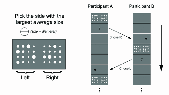
Figure 12: Two arrays of circles were given to each pair of participants on a screen. Their task is to interactively determine which side (either left or right) had the larger average diameter. The partner’s previous decision was displayed on screen prior to the stimulus.

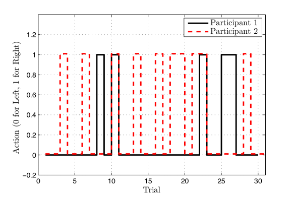
Figure 13: Example of sample path of actions chosen by two participants in a single trial of the experiment. In this trial, both participants eventually chose the correct answer 0 (left).

3.7.2 Experimental Results

The results of our experimental study are as follows:

Social learning Model

As mentioned above, the experiment for each pair of participants was continued until both participants’ responses stabilized. In what percentage of these experiments, did an agreement occur between the two participants? The answer to this question reveals whether “herding" occurred in the experiments and whether the participants performed social learning (influenced by their partners). The experiments show that in 66% of trials (1102 among 1658), participants reached an agreement; that is herding occurred. Further, in 32% of the trials, both participants converged to the correct decision after a few interactions.

To construct a social learning model for the experimental data, we consider the experiments where both participants reached an agreement. Define the social learning success rate as

$$\frac{\text{\# expts where both participants chose correct answer}}{\text{\# expts where both participants reached an agreement}}\cdot$$

In the experimental study, the state space is $\mathbb{X}=\{0,1\}$ where $x=0$, when the left array of circles has the larger diameter and $x=1$, when the right array has the larger diameter. The initial belief for both participants is considered to be $\pi_{0}=[0.5,0.5]$. The observation space is assumed to be $\mathbb{Y}=\{0,1\}$.

To estimate the social learning model parameters (observation probabilities $B_{iy}$ and costs $c(i,a)$), we determined the parameters that best fit the learning success rate of the experimental data. The best fit parameters obtained were

$$B_{iy}=\begin{bmatrix}0.61&0.39\\ 0.41&0.59\end{bmatrix},\quad c(i,a)=\begin{bmatrix}0&2\\ 2&0\end{bmatrix}.$$

Note that $B_{iy}$ and $c(i,a)$ satisfy both the conditions of the Theorem 3.5, namely TP2 observation probabilities and single-crossing cost. This implies that the subjects of this experiment made monotone and ordinal decisions.

Data incest

Here, we study the effect of information patterns in the experimental study that can result in data incest. Since private observations are highly subjective and participants did not document these, we cannot claim with certainty if data incest changed the action of an individual. However, from the experimental data, we can localize specific information patterns that can result in incest. In particular, we focus on the two information flow graphs depicted in Fig.14. In the two graphs of Fig.14, the action of the first participant at time $k$ influenced the action of the second participant at time $k+1$, and thus, could have been double counted by the first participant at time $k+2$. We found that in 79% of experiments, one of the information patterns shown in Fig.14 occurred (1303 out of 1658 experiments). Further, in 21% of experiments, the information patterns shown in Fig.14 occurred and at least one participant changed his/her decision, i.e., the judgement of participant at time $k+1$ differed from his/her judgements at time $k+2$ and $k$. These results show that even for experiments involving two participants, data incest information patterns occur frequently (79%) and causes individuals to modify their actions (21%). It shows that social learning protocols require careful design to handle and mitigate data incest.

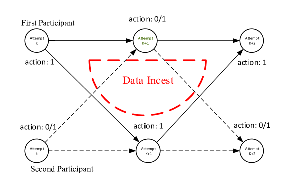
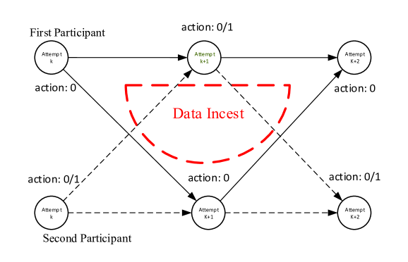
Figure 14: Two information patterns from our experimental studies which can result in data incest.

3.8 Summary and Extensions

In this section, we have outlined a controlled sensing problem over a social network in which the administrator controls (removes) data incest and thereby maintains an unbiased (fair) online reputation system. The state of nature could be geographical coordinates of an event (in a target localization problem) or quality of a social unit (in an online reputation system). As discussed above, data incest arises due to the recursive nature of Bayesian estimation and non-determinism in the timing of the sensing by individuals. Details of proofs, extensions and further numerical studies are presented in [110, 77].

We summarize some extensions of the social learning framework that are relevant to interactive sensing.

3.8.1 Wisdom of Crowds

Surowiecki’s book [168] is an excellent popular piece that explains the wisdom-of-crowds hypothesis. The wisdom-of-crowds hypothesis predicts that the independent judgments of a crowd of individuals (as measured by any form of central tendency) will be relatively accurate, even when most of the individuals in the crowd are ignorant and error prone. The book also studies situations (such as rational bubbles) in which crowds are not wiser than individuals. Collect enough people on a street corner staring at the sky, and everyone who walks past will look up. Such herding behavior is typical in social learning.

3.8.2 In which order should agents act?

In the social learning protocol, we assumed that the agents act sequentially in a pre-defined order. However, in many social networking applications, it is important to optimize the order in which agents act. For example, consider an online review site where individual reviewers with different reputations make their reviews publicly available. If a reviewer with high reputation publishes her review first, this review will unduly affect the decision of a reviewer with lower reputation. In other words, if the most senior agent “speaks" first it would unduly affect the decisions of more junior agents. This could lead to an increase in bias of the underlying state estimate. On the other hand, if the most junior agent is polled first, then since its variance is large, several agents would need to be polled in order to reduce the variance. We refer the reader to [148] for an interesting description of who should speak first in a public debate. It turns out that for two agents, the seniority rule is always optimal for any prior – that is, the senior agent speaks first followed by the junior agent; see [148] for the proof. However, for more than two agents, the optimal order depends on the prior, and the observations in general.

4 Revealed Preferences: Are social sensors utility maximizers?

We now move on to the third main topic of the chapter, namely, the principle of revealed preferences. The main question addressed is: Given a dataset of decisions made by a social sensor, is it possible to determine if the social sensor is a utility maximizer? More generally, is a dataset from a multiagent system consistent with play from a Nash equilibrium? If yes, can the behavior of the social sensors be learned using data from the social network?

These questions are fundamentally different to the model-based theme that is widely used in the signal processing literature in which an objective function (typically convex) is proposed and then algorithms are constructed to compute the minimum. In contrast, the revealed preference approach is data-centric–we wish to determine whether the dataset is obtained from an utility maximizer. In simple terms, revealed preference theory seeks to determine if an agent is an utility maximizer subject to budget constraints based on observing its choices over time. In signal processing terminology, such problems can be viewed as set-valued system identification of an argmax nonlinear system. The principle of revealed preferences is widely studied in the micro-economics literature. As mentioned in Sec.1, Varian has written several influential papers in this area. In this section we will use the principle of revealed preferences on datasets to determine how social sensors behave as a function of external influence. The setup is depicted in the schematic diagram Fig.15.

4.1 Afriat’s Theorem for a single agent

The theory of revealed preferences was pioneered by Samuelson [163]. Afriat published a highly influential paper [7] in revealed preferences (see also [8]). Given a time-series of data $\mathcal{D}=\{(p_{t},x_{t}),t\in\{1,2,\dots,T\}\}$ where $p_{t}\in\mathds{R}^{m}$ denotes the external influence, $x_{t}$ denotes the response of agent, and $t$ denotes the time index, is it possible to detect if the agent is a utility maximizer? An agent is a utility maximizer if for every external influence $p_{t}$, the chosen response $x_{t}$ satisfies

$$x_{t}(p_{t})\in\operatorname*{arg\,max}_{\{p_{t}^{\prime}x\leq I_{t}\}}u(x)$$ (50)

with $u(x)$ a non-satiated utility function. Nonsatiated means that an increase in any element of response $x$ results in the utility function increasing. As shown by Diewert [54], without local nonsatiation the maximization problem (50) may have no solution.

In (50) the budget constraint $p_{t}^{\prime}x\leq I_{t}$ denotes the total amount of resources available to the social sensor for selecting the response $x$ to the external influence $p_{t}$. For example, if $p_{t}$ is the electricity price and $x_{t}$ the associated electricity consumption, then the budget of the social sensor is the available monetary funds for purchasing electricity. In the real-world social sensor datasets provided in this chapter, further insights are provided for the budget constraint.

The celebrated “Afriat’s theorem" provides a necessary and sufficient condition for a finite dataset $\mathcal{D}$ to have originated from an utility maximizer. Afriat’s theorem has subsequently been expanded and refined, most notably by Diewert [54], Varian [175] and Blundell [26].

Theorem 4.1 (Afriat’s Theorem).

Given a dataset $\mathcal{D}=\{(p_{t},x_{t}):t\in\{1,2,\dots,T\}\}$, the following statements are equivalent:

1. The agent is a utility maximizer and there exists a nonsatiated and concave utility function that satisfies (50).

2. For scalars $u_{t}$ and $\lambda_{t}>0$ the following set of inequalities has a feasible solution:

   $$u_{\tau}-u_{t}-\lambda_{t}p_{t}^{\prime}(x_{\tau}-x_{t})\leq 0\text{ for }t,\tau\in\{1,2,\dots,T\}.\$$ (51)

3. A nonsatiated and concave utility function that satisfies (50) is given by:

   $$u(x)=\underset{t\in T}{\operatorname{min}}\{u_{t}+\lambda_{t}p_{t}^{\prime}(x-x_{t})\}$$ (52)

4. The dataset $\mathcal{D}$ satisfies the Generalized Axiom of Revealed Preference (GARP), namely for any $k\leq T$, $p_{t}^{\prime}x_{t}\geq p_{t}^{\prime}x_{t+1}\quad\forall t\leq k-1\implies p_{k}^{\prime}x_{k}\leq p_{k}^{\prime}x_{1}.$ ∎

As pointed out in [175], a remarkable feature of Afriat’s theorem is that if the dataset can be rationalized by a non-trivial utility function, then it can be rationalized by a continuous, concave, monotonic utility function. “Put another way, violations of continuity, concavity, or monotonicity cannot be detected with only a finite number of demand observations".

Verifying GARP (statement 4 of Theorem 4.1) on a dataset $\mathcal{D}$ comprising $T$ points can be done using Warshall’s algorithm with $O(T^{3})$ [175, 62] computations. Alternatively, determining if Afriat’s inequalities (51) are feasible can be done via a LP feasibility test (using for example interior point methods [31]). Note that the utility (52) is not unique and is ordinal by construction. Ordinal means that any monotone increasing transformation of the utility function will also satisfy Afriat’s theorem. Therefore the utility mimics the ordinal behavior of humans, see also Sec.3.6. Geometrically the estimated utility (52) is the lower envelop of a finite number of hyperplanes that is consistent with the dataset $\mathcal{D}$.

Note that GARP is equivalent to the notion of “cyclical consistency” [176] – they state that the responses are consistent with utility maximization if no negative cycles are present. As an example, consider a dataset $\mathcal{D}$ with $T=2$ observations resulting from a utility maximization agent. Then GARP states that $p_{1}^{\prime}x_{1}\geq p_{1}^{\prime}x_{2}$ $\implies p_{2}^{\prime}x_{2}\leq p_{2}^{\prime}x_{1}$. From (50), the underlying utility function must satisfy $u(x_{1})\geq u(x_{2})$ $\implies u(x_{2})\leq u(x_{1})$ where the equality results if $x_{1}=x_{2}$.

Another remarkable feature of Afriat’s Theorem is that no parametric assumptions of the utility function of the agent are necessary. To gain insight into the construction of the inequalities (51), let us assume the utility function $u(x)$ in (50) is increasing for positive $x$, concave, and differentiable. If $x_{t}$ solves the maximization problem (50), then from the Karush-Kuhn-Tucker (KKT) conditions there must exist Lagrange multipliers $\lambda_{t}$ such that

$$\nabla u(x_{t})=\lambda_{t}\nabla(p_{t}^{\prime}x_{t}-I_{t})=\lambda_{t}p_{t}$$

is satisfied for all $t\in\{1,2,\dots,T\}$. Note that since $u(x)$ is increasing, $\nabla u(x_{t})=\lambda_{t}p_{t}>0$, and since $p_{t}$ is strictly positive, $\lambda_{t}>0$. Given that $u(x)$ is a concave differentiable function, it follows that

$$u(x)\leq u(x_{t})+\nabla u(x_{t})^{\prime}(x-x_{t})\quad\forall t\in\{1,2,\dots,T\}.$$

Denoting $u_{t}=u(x_{t})$ and $u_{\tau}=u(x_{\tau})$, and using the KKT conditions and concave differential property, the inequalities (51) result. To prove that if the solution of (51) is feasible then GARP is satisfied can be performed using the duality theorem of linear programming as illustrated in [62].

4.2 Revealed Preferences for Multi-agent Social Sensors

We now consider a multi-agent version of Afriat’s theorem for deciding if a dataset is generated by playing from the equilibrium of a potential game An example is the control of power consumption in the electrical grid. Consider a corporate network of financial management operators that select the electricity prices in a set of zones in the power grid. By selecting the prices of electricity the operators are expected to be able to control the power consumption in each zone. The operators wish to supply their consumers with sufficient power however given the finite amount of resources the operators in the corporate network must interact. This behavior can be modelled as a game. Recent analysis of energy use scheduling and demand side management schemes in the energy market have been performed using potential games [38, 91, 184]. Another example of potential games are congestion games [160, 81, 17, 135] in which the utility of each player depends on the amount of resource it and other players use.

Consider the social network presented in Fig.15, given a time-series of data from $N$ agents $\mathcal{D}=\{(p_{t},x_{t}^{1},\dots,x_{t}^{n}):t\in\{1,2,\dots,T\}\}$ with $p_{t}\in\mathds{R}^{m}$ the external influence, $x_{t}^{i}$ the response of agent $i$, and $t$ the time index, is it possible to detect if the dataset originated from agents that play a potential game?

The characterization of how agents behave as a function of external influence, for example price of using a resource, and the responses of other agents in a social network, is key for analysis. Consider the social network illustrated in Fig.15. There are a total of $n$ interacting agents in the network and each can produce a response $x_{t}^{i}$ in response to the other agents and an external influence $p_{t}$. Without any a priori assumptions about the agents, how can the behaviour of the agents in the social network be learned? In the engineering literature the behaviour of agents is typically defined a priori using a utility function, however our focus here is on learning the behaviour of agents. The utility function captures the satisfaction or payoff an agent receives from a set of possible responses, denoted by $X$. Formally, a utility function $u:X\rightarrow\mathds{R}$ represents a preference relation between responses $x_{1}$ and $x_{2}$ if and only if for every $x_{1},x_{2}\in X$, $u(x_{1})\leq u(x_{2})$ implies $x_{2}$ is preferred to $x_{1}$. Given a time-series of data $\mathcal{D}=\{(p_{t},x_{t}^{1},\dots,x_{t}^{n}):t\in\{1,2,\dots,T\}\}$ with $p_{t}\in\mathds{R}^{m}$ the external influence, $x_{t}^{i}$ the response of agent $i$, and $t$ the time index, is it possible to detect if the series originated from an agent that is a utility maximizer?

Figure 15: Schematic of a social network containing $n$ agents where $p_{t}\in\mathds{R}^{m}$ denotes the external influence, and $x_{t}^{i}\in\mathds{R}^{m}$ the response of agent $i$ in response to the external influence and other agents at time $t$. Note that dotted line denotes consumers $4,\dots,n-1$. The aim is to determine if the dataset $\mathcal{D}$ defined in (53), is consistent with play from a Nash equilibrium.

In a network of social sensors (Fig.15), the responses of agents may be dependent on both the external influence $p_{t}$ and the responses of the other agents in the network, denoted by $x_{t}^{-i}$. The utility function of the agent must now include the responses of other agents–formally if there are $n$ agents, each has a utility function $u^{i}(x^{i},x_{t}^{-i})$ with $x^{i}$ denoting the response of agent $i$, $x_{t}^{-i}$ the responses of the other $n-1$ agents, and $u^{i}(\cdot)$ the utility of agent $i$. Given a dataset $\mathcal{D}$, is it possible to detect if the data is consistent with agents playing a game and maximizing their individual utilities? Deb, following Varian’s and Afriat’s work, shows that refutable restrictions exist for the dataset $\mathcal{D}$, given by (53), to satisfy Nash equilibrium (54) [51, 7, 178]. These refutable restrictions are however, satisfied by most $\mathcal{D}$ [51]. The detection of agents engaged in a concave potential game, and generating responses that satisfy Nash equilibrium, provide stronger restrictions on the dataset $\mathcal{D}$ [51, 52]. We denote this behaviour as Nash rationality, defined as follows:

Definition 4.2 ([52, 174, 145]).

Given a dataset

$$\mathcal{D}=\{(p_{t},x_{t}^{1},x_{t}^{2},\dots,x_{t}^{n}):t\in\{1,2,\dots,T\}\},$$ (53)

$\mathcal{D}$ is consistent with Nash equilibrium play if there exist utility functions $u^{i}(x^{i},x^{-i})$ such that

$$x_{t}^{i}=x_{t}^{i*}(p_{t})\in\operatorname*{arg\,max}_{\{p_{t}^{\prime}x^{i}\leq I_{t}^{i}\}}u^{i}(x^{i},x^{-i}).$$ (54)

In (54), $u^{i}(x,x^{-i})$ is a nonsatiated utility function in $x$, $x^{-i}=\{x^{j}\}_{j\neq i}$ for $i,j\in\{1,2,\dots,n\}$, and the elements of $p_{t}$ are strictly positive. Nonsatiated means that for any $\epsilon>0$, there exists a $x^{i}$ with $\lVert x^{i}-x^{i}_{t}\rVert_{2}<\epsilon$ such that $u^{i}(x^{i},x^{-i})>u^{i}(x_{t}^{i},x_{t}^{-i})$. If for all $x^{i},x^{j}\in X^{i}$, there exists a concave potential function $V$ that satisfies

$$u^{i}(x^{i},x^{-i})-u^{i}(x^{j},x^{-i})>0\text{ iff }V(x^{i},x^{-i})-V(x^{j},x^{-i})>0$$ (55)

for all the utility functions $u^{i}(\cdot)$ with $i\in\{1,2,\dots,n\}$, then the dataset $\mathcal{D}$ satisfies Nash rationality. ∎

Just as with the utility maximization budget constraint in (50), the budget constraint $p_{t}^{\prime}x^{i}\leq I_{t}^{i}$ in (54) models the total amount of resources available to the social sensor for selecting the response $x^{i}_{t}$ to the external influence $p_{t}$.

The detection test for Nash rationality (Definition 4.2) has been used in [35] to detect if oil producing countries are collusive, and in [51] for the analysis of household consumption behaviour.

In the following sections, decision tests for utility maximization, and a non-parametric learning algorithm for predicting agent responses are presented. Three real world datasets are analyzed using the non-parametric decision tests and learning algorithm. The datasets are comprised of bidders auctioning behaviour, electrical consumption in the power grid, and on the tweeting dynamics of agents in the social network Twitter illustrated in Fig.15.

4.3 Decision Test for Nash Rationality

This section presents a non-parametric test for Nash rationality given the dataset $\mathcal{D}$ defined in (53). If the dataset $\mathcal{D}$ passes the test, then it is consistent with play according to a Nash equilibrium of a concave potential game. In Sec.4.4, a learning algorithm is provided that can be used to predict the response of agents in the social network provided in Fig.15.

The following theorem provides necessary and sufficient conditions for a dataset $\mathcal{D}$ to be consistent with Nash rationality (Definition 4.2). The proof is analogous to Afriat’s Theorem when the concave potential function of the game is differentiable [51, 52, 89].

Theorem 4.3 (Multiagent Afriat’s Theorem).

Given a dataset $\mathcal{D}$ (53), the following statements are equivalent:

1. $\mathcal{D}$ is consistent with Nash rationality (Definition 4.2) for an $n$-player concave potential game.

2. Given scalars $v_{t}$ and $\lambda_{t}^{i}>0$ the following set of inequalities have a feasible solution for $t,\tau\in\{1,\dots,T\},$

   $$v_{\tau}-v_{t}-\sum\limits_{i=1}^{n}\lambda_{t}^{i}p_{t}^{\prime}(x_{\tau}^{i}-x_{t}^{i})\leq 0.\quad$$ (56)

3. A concave potential function that satisfies (54) is given by:

   $$\hat{V}(x^{1},x^{2},\dots,x^{n})=\underset{t\in T}{\operatorname{min}}\{v_{t}+\sum_{i=1}^{n}\lambda_{t}^{i}p_{t}^{\prime}(x^{i}-x^{i}_{t})\}.$$ (57)

4. The dataset $\mathcal{D}$ satisfies the Potential Generalized Axiom of Revealed Preference (PGARP) if the following two conditions are satisfied.

   1. For every dataset $\mathcal{D}_{\tau}^{i}=\{(p_{t},x_{t}^{i}):t\in\{1,2,\dots,\tau\}\}$ for all $i\in\{1,\dots,n\}$ and all $\tau\in\{1,\dots,T\},$ $\mathcal{D}_{\tau}^{i}$ satisfies GARP.

   2. The responses $x_{t}^{i}$ originated from players in a concave potential game. ∎

Note that if only a single agent (i.e. $n=1$) is considered, then Theorem 4.3 is identical to Afriat’s Theorem. Similar to Afriat’s Theorem, the constructed concave potential function (57) is ordinal–that is, unique up to positive monotone transformations. Therefore several possible options for $\hat{V}(\cdot)$ exist that would produce identical preference relations to the actual potential function $V(\cdot)$. In 4) of Theorem 4.3, the first condition only provides necessary and sufficient conditions for the dataset $\mathcal{D}$ to be consistent with a Nash equilibrium of a game, therefore the second condition is required to ensure consistency with the other statements in the Multiagent Afriat’s Theorem. The intuition that connects statements 1 and 3 in Theorem 4.3 is provided by the following result from [145]; for any smooth potential game that admits a concave potential function $V$, a sequence of responses $\{x^{i}\}_{i\in\{1,2,\dots,n\}}$ are generated by a pure-strategy Nash equilibrium if and only if it is a maximizer of the potential function,

$$x_{t}=\{x_{t}^{1},x_{t}^{2},\dots,x_{t}^{n}\}\in\operatorname*{arg\,max}V(\{x^{i}\}_{i\in\{1,2,\dots,n\}})$$

$$\text{s.t. }\quad p_{t}^{\prime}x^{i}\leq I_{t}^{i}\quad\quad\forall i\in\{1,2,\dots,n\}$$ (58)

for each probe vector $p_{t}\in\mathds{R}_{+}^{m}$.

The non-parametric test for Nash rationality involves determining if (56) has a feasible solution. Computing parameters $v_{t}$ and $\lambda^{i}_{t}>0$ in (56) involves solving a linear program with $T^{2}$ linear constraints in $(n+1)T$ variables, which has polynomial time complexity [31]. In the special case of one agent, the constraint set in (56) is the dual of the shortest path problem in network flows. Using the graph theoretic algorithm presented in [20], the solution of the parameters $u_{t}$ and $\lambda_{t}$ in (51) can be computed with time complexity $O(T^{3})$.

4.4 Learning Algorithm for Response Prediction

In the previous section a non-parametric tests to detect if a dataset $\mathcal{D}$ is consistent with Nash rationality was provided. If the $\mathcal{D}$ satisfies Nash rationality, then the Multiagent Afriat’s Theorem can be used to construct the concave potential function of the game for agents in the social network illustrated in Fig.15. In this section we provide a non-parametric learning algorithm that can be used to predict the responses of agents using the constructed concave potential function (57).

To predict the response of agent $i$, denoted by $\hat{x}_{\tau}^{i}$, for probe $p_{\tau}$ and budget $I_{\tau}^{i}$, the optimization problem (58) is solved using the estimated potential function $\hat{V}$ (57), $p_{\tau}$, and $I_{\tau}^{i}$. Computing $\hat{x}_{\tau}^{i}$ requires solving an optimization problem with linear constraints and concave piecewise linear objective. This can be solved using the interior point algorithm [31]. The algorithm used to predict the response $\hat{x}_{\tau}=(\hat{x}_{\tau}^{1},\hat{x}_{\tau}^{2},\cdots,\hat{x}_{\tau}^{n})$ is given below: [0mm]0mm

1. Select a probe vector $p_{\tau}\in\mathds{R}^{m}_{+}$, and response budget $I_{\tau}^{i}$ for the estimation of optimal response $\hat{x}_{\tau}\in\mathds{R}_{+}^{m\times n}$.

2. For dataset $\mathcal{D}$, compute the parameters $v_{t}$ and $\lambda_{t}^{i}$ using (56).

3. The response $\hat{x}_{\tau}$ is computed by solving the following linear program given $\{\mathcal{D},p_{\tau},I_{\tau}^{i}\}$, and $\{v_{t},\lambda_{t}^{i}\}$ from Step 2:

   $$\begin{array}[]{rl}\max&z\\ \mbox{s.t.}&z\leq v_{t}+\sum\limits_{i=1}^{n}\lambda_{t}^{i}p_{t}^{\prime}(\hat{x}^{i}_{\tau}-x^{i}_{t})\text{ for }t=1,\dots,T\\ &p_{\tau}^{\prime}\hat{x}^{i}_{\tau}\leq I^{i}_{\tau}\quad\forall i\in\{1,2,\dots,n\}\end{array}$$ (59)

4.5 Dataset 1: Online Multiwinner Auction

This section illustrates how Afriat’s Theorem from Sec.4.1 can be used to determine if bidders in an online multiwinner auction are utility optimizers. Online auctions are rapidly gaining popularity since bidders do not have to gather at the same geographical location. Several researchers have focused on the timing of bids and multiple bidding behavior in Amazon and eBay auctions [30, 147, 155, 53]. The analysis of the bidding behavior can be exploited by auctioneers to target suitable bidders and thereby increase profits.

The multiwinner auction dataset was obtained from an experimental study conducted amongst undergraduate students in Electrical Engineering at Princeton University in March $25^{\text{th}}$ 2011. The multiwinner auction consists of bidders competing for questions that will aid them for an upcoming midterm exam. The social network is composed of $n=12$ bidders where the bidders do not interact with other bidders, they only interact with the external influence, refer to Fig.15. Each bidder is endowed with 500 tokens prior to starting the multiwinner auction. The number of questions being auctioned is not known to the bidders, this prevents the bidders from immediately submitting their entire budget in the final auction. Each auction consists of auctioning a single question at an initial price of 10 tokens and has a duration of 30 min. At the beginning of each auction the bidders are provided with the number of winners, denoted $k$, that auction will have, and the budget of each bidder. The bids are private information with each bidder only informed when their bid has been outbid. The bidders do not communicate with each other during the auction. At the end of each auction, the first $k$ highest bidders are selected, denoted by $\zeta_{1},\zeta_{2},\dots,\zeta_{k}$. The bidders $\zeta_{1},\zeta_{2},\dots,\zeta_{k}$ are awarded with the question, and pay the second largest bid amount (i.e. bidder $\zeta_{k}$ pays $\zeta_{k-1}$’s bid amount). In the multiwinner auction it is in the self interest of bidders to force other bidders to spend too much eliminating them from competing in successive auctions.

If the bidding behaviour of agents satisfies Afriat’s test (51) for utility maximization, the next goal is to classify the behaviour of bidders into two categories: strategic and frantic. If a bidder fails Afriat’s test then they are classified as irrational. Strategic bidders will typically submit a large number of bids and a smaller bid amount when compared to frantic bidders. With this bidding behaviour, strategic bidders force the other bidders to spend too much eliminating them from competing in future auctions. Frantic bidders are however only interested in winning the current auction.

To apply Afriat’s test (51), the external influence $p_{t}$, and bidder responses $x_{t}$ must be defined. The external influence for each bidder is defined by $p_{t}^{i}=[p_{t}^{i}(1),p_{t}^{i}(2)]$ with $p^{i}_{t}(1)=$ initial bid amount representing the bidders interest level for winning, and $p^{i}_{t}(2)=$ # of winners representing the perception of winning where $i$ is the bidder and $t$ the auction. Two datasets are considered for analysis denoted by $\mathcal{D}_{1}$ and $\mathcal{D}_{2}$. An identical external influence is used to construct both $\mathcal{D}_{1}$ and $\mathcal{D}_{2}$. The responses in $\mathcal{D}_{1}$ are given by $x_{t}^{i}=[x_{t}^{i}(1),x_{t}^{i}(2)]$ where $x_{t}^{i}(1)=$ # of bids and $x_{t}^{i}(2)=$ mean bid amount; and for $\mathcal{D}_{2}$ the inputs of $x_{t}^{i}$ are given by $x_{t}^{i}(1)=$ # of bids and $x_{t}^{i}(2)=$ mean change in bid amount. The response $x_{t}^{i}(2)$ in $\mathcal{D}_{1}$ provides the expected bid amount, and $x_{t}^{i}(2)$ in $\mathcal{D}_{2}$ a measure of the statistical dispersion of the bids. The budget $I_{t}^{i}$ of each bidder has units of tokens multiplied by # of bids, and is constrained as the number of tokens and auction duration are finite. The datasets $\mathcal{D}_{1}$ and $\mathcal{D}_{2}$ are constructed from $T=6$ auctions. The non-parametric test (51) is applied to each dataset $\mathcal{D}_{1}$ and $\mathcal{D}_{2}$ to detect irrational bidders. For dataset $\mathcal{D}_{1}$ bidder 4 is irrational, and for $\mathcal{D}_{2}$ bidder 11 is irrational. Note that the classification of irrational behaviour is dependent on the choice of response signals used for analysis by the experimentalist.

For utility maximization bidders, an estimate of the utility function of each bidder is required to classify them as strategic or frantic. To estimate the utility function of the bidders, a subset of data from $\mathcal{D}_{1}$, denoted as $\bar{\mathcal{D}}_{1}$, is selected such that the preferences of all agents $i$ in $\bar{\mathcal{D}}_{1}$ are identical. It was determined that $\bar{\mathcal{D}}_{1}=\{(p_{t}^{i},x_{t}^{i}):i\in\{1,3,5,7,12\}\}$. Since the preferences of these bidders are identical, we can consider all the data in $\bar{\mathcal{D}}_{1}$ as originating from a single representative bidder. This allows an improved estimate of the utility function of these bidders as compared to learning the utility function for each bidder separately. An analogous explanation is used for the construction of $\bar{\mathcal{D}}_{2}=\{(p_{t}^{i},x_{t}^{i}):i\in\{1,2,3,4,7,8,9\}\}$ from the dataset $\mathcal{D}_{2}$. The estimated utility function for $\bar{\mathcal{D}}_{1}$ is given in Fig.16(a) and for $\bar{\mathcal{D}}_{2}$ in Fig.16(b). As seen from Fig.16(a) and Fig.16(b), bidders have a preference to increase the number of bids compared with increasing the mean bid amount or the difference in mean bid amount. This follows logically as $x_{t}^{i}(2)$ increases, the bidder will have to pay more tokens to win the question limiting their ability to bid in future auctions. Interestingly, the bidders show strategic and frantic behaviour in both datasets $\mathcal{\bar{D}}_{1}$ and $\mathcal{\bar{D}}_{2}$, as seen in Fig.16(a) and Fig.16(b). This is consistent with the results in [155] which show that bidders change their bidding behavior between successive auctions.

The analysis shows that auctioneers should target bidders that show frantic bidding behavior as they are likely to overspend on items increasing the revenue of the auctioneer. Such behavior can be detected using utility maximization test and constructed utility function from Afriat’s Theorem.

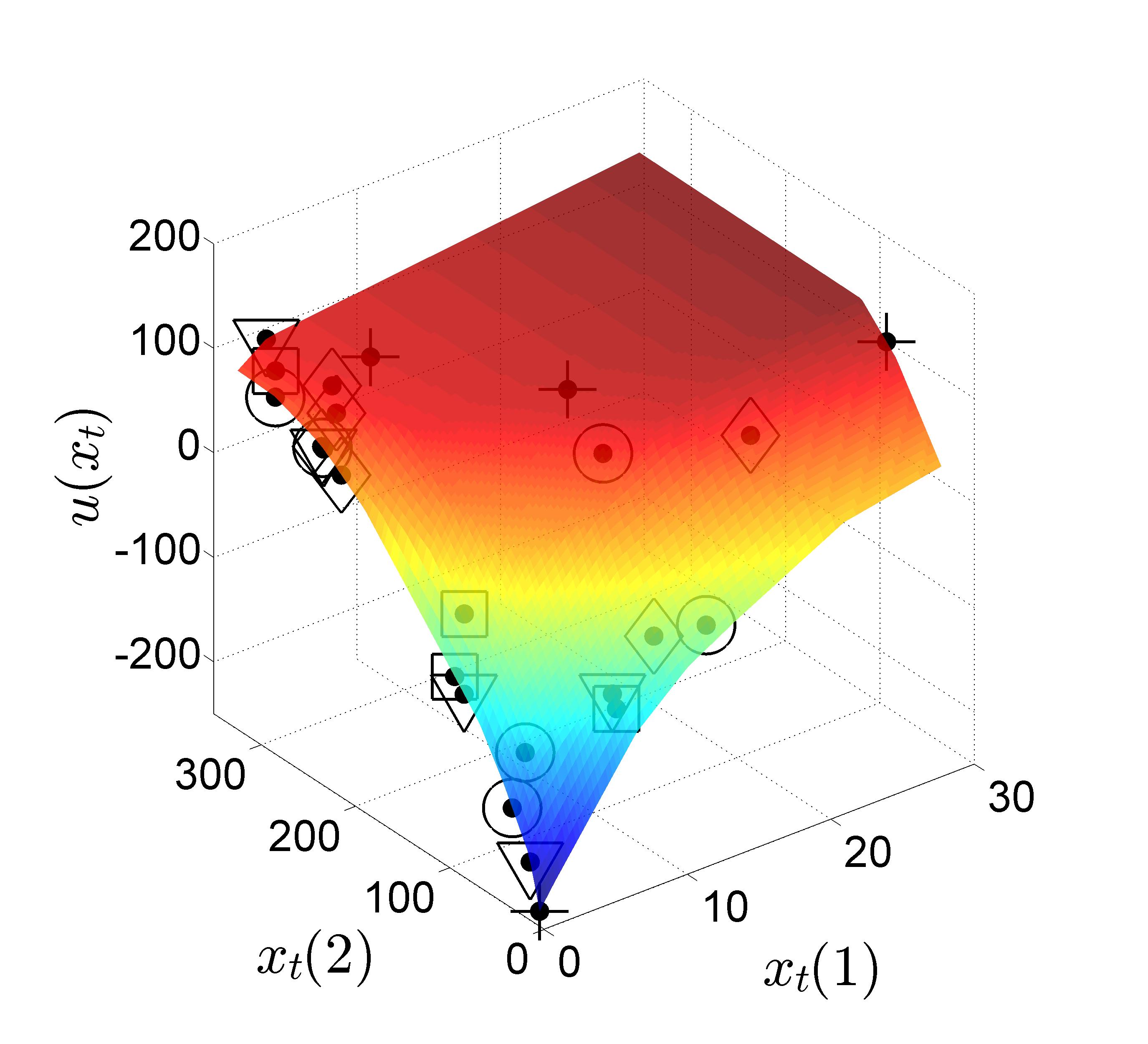
(a) Estimated utility function $u(x_{t})$ using dataset $\bar{\mathcal{D}}_{1}$ defined in Sec.4.5.

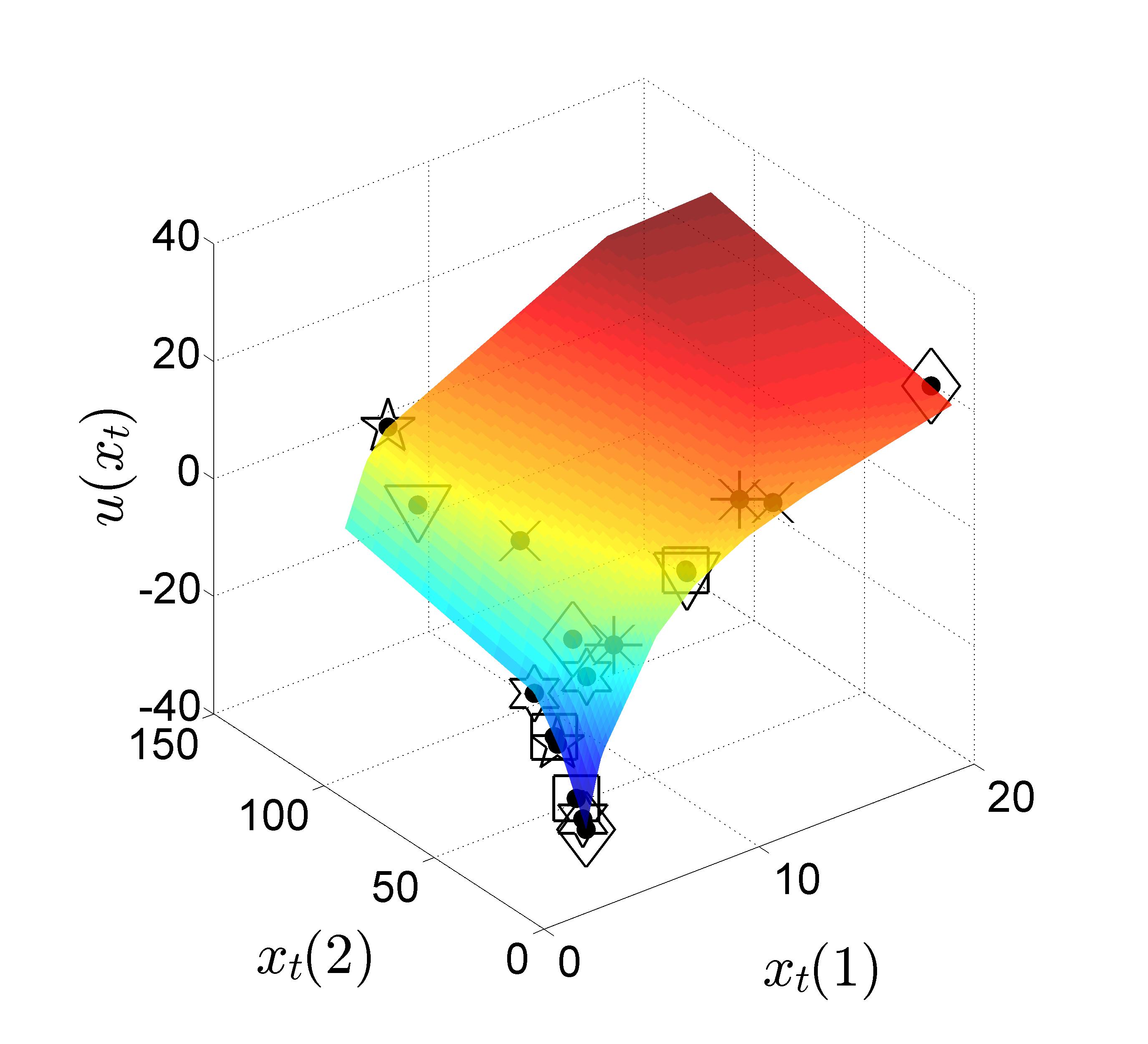
(b) Estimated utility function $u(x_{t})$ using dataset $\bar{\mathcal{D}}_{2}$ defined in Sec.4.5.

Figure 16: Estimated utility function of bidders is constructed using (52) using the datasets $\bar{\mathcal{D}}_{1}$ and $\bar{\mathcal{D}}_{2}$ defined in Sec.4.5. The black dots represent the utility associated with experimentally measured responses, and the colour (blue to red) indicates the utility level. The black dots indicate the observed demands, and the shape (i.e. circle, diamond etc.) denotes the respective bidder.

4.6 Dataset 2: Ontario Electrical Energy Market Dataset

In this section we consider the aggregate power consumption of different zones in the Ontario power grid. A sampling period of $T=79$ days starting from January 2013 is used to generate the dataset $\mathcal{D}$ for the analysis. All price and power consumption data is available from the Independent Electricity System Operator (IESO) website. Each zone is considered as an agent in the corporate network illustrated in Fig.15. The study of corporate social networks was pioneered by Granovetter [73, 74] which shows that the social structure of the network can have important economic outcomes. Examples include agents choice of alliance partners, assumption of rational behavior, self interest behavior, and the learning of other agents behavior. Here we test for rational behavior (i.e. utility maximization and Nash rationality), and if true then learn the associated behavior of the zones. This analysis provides useful information for constructing demand side management (DSM) strategies for controlling power consumption in the electricity market. For example, if a utility function exists it can be used in the DSM strategy presented in [50, 146].

The zones power consumption is regulated by the associated price of electricity set by the senior management officer in each respective zone. Since there is a finite amount of power in the grid, each officer must communicate with other officers in the network to set the price of electricity. Here we utilize the aggregate power consumption from each of the $n=10$ zones in the Ontario power grid and apply the non-parametric tests for utility maximization (51) and Nash rationality (56) to detect if the zones are demand responsive. If the utility maximization or Nash rationality tests are satisfied, then the power consumption behaviour is modelled by constructing the associated utility function (52) or concave potential function of the game (57).

To perform the analysis the external influence $p_{t}$ and response of agents $x_{t}$ must be defined. In the Ontario power grid the wholesale price of electricity is dependent on several factors such as consumer behaviour, weather, and economic conditions. Therefore the external influence is defined as $p_{t}=[p_{t}(1),p_{t}(2)]$ with $p_{t}(1)$ the average electricity price between midnight and noon, and $p_{t}(2)$ as the average between noon and midnight with $t$ denoting day. The response of each zone correspond to the total aggregate power consumption in each respective tie associated with $p_{t}(1)$ and $p_{t}(2)$ and is given by $x_{t}^{i}=[x_{t}^{i}(1),x_{t}^{i}(2)]$ with $i\in\{1,2,\dots,n\}$. The budget $I_{t}^{i}$ of each zone has units of dollars as $p_{t}$ has units of $/kWh and $x_{t}^{i}$ units of kWh.

We found that the aggregate consumption data of each zone does not satisfy Afriat’s utility maximization test (51). This points to the possibility that the zones are engaged in a concave potential game–this would not be a surprising result as network congestion games have been shown to reduce peak power demand in distributed demand management schemes [91]. To test if the dataset $\mathcal{D}$ is consistent with Nash rationality the detection test (56) is applied. The dataset for the power consumption in the Ontario power gird is consistent with Nash rationality. Using (59), a concave potential function for the game is constructed. Using the constructed potential function, when do agents prefer to consume power? The marginal rate of substitution (MRS) can be used to determine the preferred time for power usage. Formally, the MRS of $x^{i}(1)$ for $x^{i}(2)$ is given by

$$\operatorname{MRS}_{12}=\frac{\partial\hat{V}/\partial x^{i}(1)}{\partial\hat{V}/\partial x^{i}(2)}.$$

From the constructed potential function we find that $\operatorname{MRS}_{12}>1$ suggesting that the agents prefer to use power in the time period associated with $x_{t}(1)$–that is, the agents are willing to give up $\operatorname{MRS}_{12}$ kWh of power in the time period associated with $x^{i}(2)$ for 1 additional kWh of power in time period associated with $x^{i}(1)$.

The analysis in this section suggests that the power consumption behavior of agents is consistent with players engaged in a concave potential game. Using the Multiagent Afriat’s Theorem the agents preference for using power was estimated. This information can be used to improve the DSM strategies presented in [50, 146] to control power consumption in the electricity market.

4.7 Dataset 3: Twitter Data

Does the tweeting behaviour of Twitter agents satisfy a utility maximization process? The goal is to investigate how tweets and trend indices impact the tweets of agents in the Twitter social network. The information provided by this analysis can be used in social media marketing strategies to improve a brand and for brand awareness. As discussed in [68], Twitter may relay on a huge amount of agent-generated data which can be analyzed to provide novel personal advertising to agents.

To apply Afriat’s utility maximization test (51), we choose the external influence and response as follows. External influence $p_{t}=[\text{\it\#Sony},1/\text{\it\#Playstation}]$ for each day $t$. The associated response taken by the agents in the network is given by $x_{t}=[\text{\it\#Microsoft},\text{\it\#Xbox}]$. Notice that the probe $p_{t}(2)$ can be interpreted as the frequency of tweets with the word Playstation (i.e. the trending index). The dataset $\mathcal{D}$ of external influence and responses is constructed from $T=80$ days of Twitter data starting from January 1${}^{\text{st}}$ 2013. The dataset $\mathcal{D}$ satisfies the utility maximization test (51). This establishes that utility function exists for agents that is dependent on the number of tweets containing the words Microsoft and Xbox. The data shows that tweets containing the word Microsoft and Xbox are dependent on the number of tweets containing Sony and trending index of Playstation. This dependency is expected as Microsoft produces the game console Xbox, and Sony produces the game console Playstation both which have a large number of brand followers (e.g. Xbox has over 3 million, and Playstation over 4 million). To gain further insight into the behaviour of the agents, (52) from Afriat’s Theorem is used to construct a utility function for the agents. Fig.17 shows the constructed utility function of the agents. As seen, agents have a higher utility for using the word Microsoft as compared to Xbox–that is, agents prefer to use the word Microsoft to that of Xbox. Interestingly, if we define the response to be $x_{t}=[\text{\it\#Microsoft},1/\text{\it\#Xbox}]$, then the dataset satisfies utility maximization. From the constructed utility function, not shown, the agents prefer to increase the tweets containing the word Microsoft compared to increasing the trend index of Xbox. If instead $x_{t}=[1/\text{\it\#Microsoft},1/\text{\it\#Xbox}]$, then the dataset satisfies utility maximization and agents prefer to increase the trend index of Microsoft compared to that of Xbox.

To summarize, the above analysis suggests the following interesting fact: Xbox has a lower utility than Microsoft in terms of Twitter sentiment. Therefore, online marketing strategies should target the brandname Microsoft instead of Xbox.

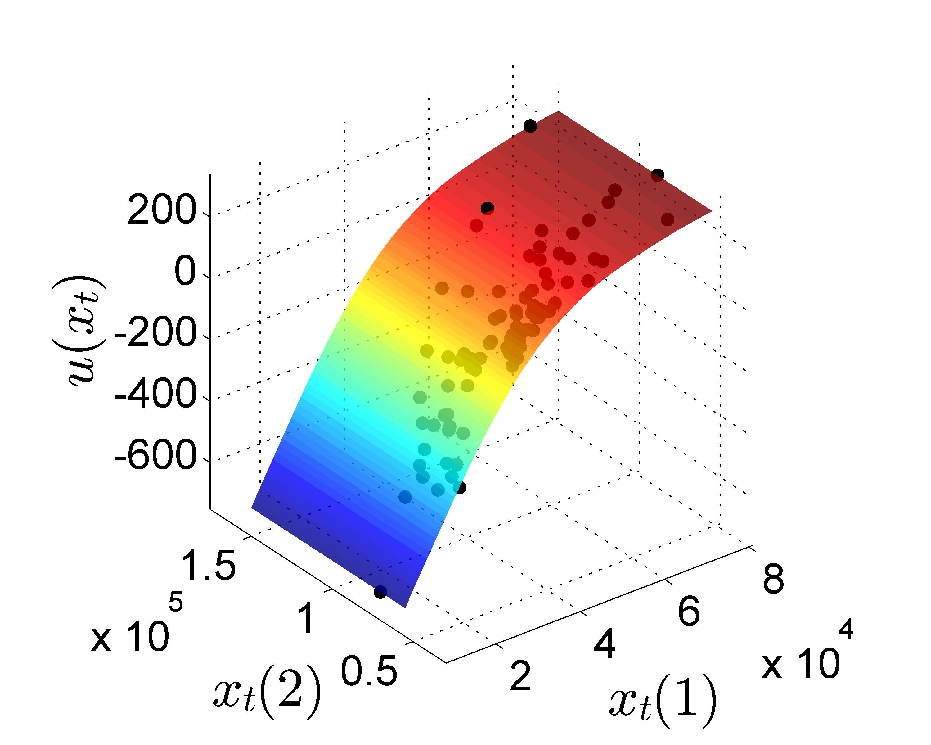
Figure 17: Estimated utility function $u(x_{t})$ using dataset $\mathcal{D}$ defined in Sec.4.7 and constructed using the non-parametric learning algorithm (52) from Afriat’s Theorem.

4.8 Summary and Extensions

The principle of revealed preferences is an active research area with numerous recent papers. We have already mentioned the papers [54, 175, 26]. Below we summarize some related literature that extends the basic framework of Afriat’s theorem.

Afriat’s theorem holds for finite datasets and gives an explicit construction of a class of concave utility functions that rationalize the dataset. Mas Colell [133] has given sufficient conditions under which as the data set size $T$ grows to infinity, the underlying utility function of the consumer can be fully identified.

Though the classical Afriat’s theorem holds for linear budget constraints $p_{t}^{\prime}x\leq I_{t}$ in (50), an identical formulation holds for certain non-linear budget constraints as illustrated in [61]. The budget constraints considered in [61] are of the form $\{x\in\mathbb{R}^{m}_{+}|g(x)\leq 0\}$ where $g:\mathbb{R}^{m}_{+}\rightarrow\mathbb{R}$ is an increasing continuous function and $\mathbb{R}^{m}_{+}$ denotes the positive orthant. Also [61] shows how the results in [133] on recoverability of the utility function can be extended to such nonlinear budget constraints. However, learning the utility function from a finite dataset in the case of a non-linear budget constraint requires sophisticated machine learning algorithms [115]. The machine learning algorithms can only guarantee that the estimated utility function is approximately consistent with the dataset $\mathcal{D}$–that is, the estimated utility is not guaranteed to contain all the preference relations consistent with the dataset $\mathcal{D}$.

In [20], results in statistical learning theory are applied to the principle of revealed preferences to address the question: Is the class of demand functions derived from monotone concave utilities efficiently probably approximately correct (PAC) learnable? It is shown that Lipschitz utility functions are efficiently PAC learnable. In [89], the authors extend the results of [20] and show that for agents engaged in a concave potential game that satisfy Nash rationality, if the underlying potential function satisfies the Lipschitz condition then the potential function of the game is PAC learnable.

In many cases, the responses of agents are observed in noise. Then determining if an agent is a utility maximizer (or a multiagent system’s response is consistent with play from a Nash) becomes a statistical decision test. In [111] it is shown how stochastic optimization algorithms can be devised to optimize the probe signals to minimize the type II errors of the decision test subject to a fixed type I error.

Change Point Detection in Utility Functions

[13] extends the classical revealed preference framework to agents with a “dynamic utility function”. The utility function jump changes at an unknown time instant by a linear perturbation. Given the dataset of probe and responses of an agent, the objective in [13] is to develop a nonparametric test to detect the change point and the utility functions before and after the change, which is henceforth referred to as the change point detection problem.

Such change point detection problems arise in online search in social media. Online search is currently the most popular method for information retrieval [166] and can be viewed as an agent maximizing the information utility, i.e. the amount of information consumed by an online agent given the limited resource on time and attention. There has been a gamut of research which links internet search behaviour to ground truths such as symptoms of illness, political election, or major sporting events [190]. Detection of utility change in online search, therefore, is helpful to identify changes in ground truth. Also, the intrinsic nature of the online search utility function motivates such a study under a revealed preference setting.

The problem of detecting a sudden linear perturbation change in the utility function is motivated by several reasons. First, the linear perturbation assumption provides sufficient selectivity such that the non-parametric test is not trivially satisfied by all datasets but still provides enough degrees of freedom. Second, the linear perturbation can be interpreted as the change in the marginal rate of utility relative to a “base” utility function. In online social media, the linear perturbation coefficients measure the impact of marketing or the measure of severity of the change in ground truth on the utility of the agent. This is similar to the linear perturbation models used to model taste changes [5, 134, 63] in microeconomics. Finally, in social networks, linear change in the utility is often used to model the change in utility of an agent based on the interaction with the agent’s neighbours [39]. Compared to the taste change model, our model is unique in that we allow the linear perturbation to be introduced at an unknown time.

A related important practical issue that we also consider in this paper is the application of revealed preference framework to high dimensional data (“big-data”). As an example of high dimensional data arising in online social media, we investigate the detection of the utility maximization process inherent in video sharing via YouTube. Detecting utility maximization behaviour with such high dimensional data is computationally demanding. [13] uses dimensionality reduction to overcome the computational cost associated with high dimensional data. The high dimensional data is projected into a lower dimensional subspace using the Johnson-Lindenstrauss (JL) transform.

5 Social Interaction of Channel Owners and YouTube Consumers

In this section time-series analysis methods are applied to real-world YouTube data to determine how social sensors interact with YouTube channel owners. Several key results are presented that elucidate the dynamics of social sensors in the YouTube social network. This section contains five main results.

1. Sec.5.2 illustrates the sensitivity of social sensor engagement to changes in meta-level (title, thumbnail, tags) features of YouTube videos. It is found that meta-level feature optimization causes an increase in user engagement for approximately 50% of videos. Optimization of the title of the video causes a significant improvement of users finding the video from YouTube search results. Additionally, optimization of the thumbnail causes an increase in users accessing the video from the related video list.

2. In Sec.5.3 Granger causality is used to show that a causal relationship exists between a channels subscriber count and the social sensor engagement of videos on the channel. However, this causal relationship is dependent on the category. For example, 80% of the “Entertainment” channels satisfy the Granger causality test while only 40% of the “Food” channels satisfy the test.

3. In Sec.5.4 it is determined that for popular gaming YouTube channels with a dominant (constant) upload schedule, deviating from the schedule increases the views and the comment counts of the channel (e.g. increases user engagement). Specifically, when the channel goes off schedule the channel gains views $97\%$ of the time and the channel gains comments $68\%$ of the time.

4. In Sec.5.5 we illustrate that the social sensor engagement dynamics with YouTube videos can be modeled using a generalized Gompertz model. The generalized Gompertz model accounts for the initial viral increase in views from subscribers, the subsequent linear growth that results from non-subscribers, and views from exogenous events such as promotion on other popular social media platforms. It is important to account for exogenous events when estimating the efficiency of meta-level optimization procedures.

5. In Sec.5.6 the generalized Gombertz model is used to study the dynamics of social sensors to video playthroughs (squence of videos on the same topic). It is illustrated that the early view count dynamics are highly correlated with the view count dynamics of future videos. Both the short term view count and long term migration of users to future videos in the playthrough decrease after the initial video in the playthrough is posted. This results even when the channels subscriber count increases. A possible reason for this decrease is that subsequent videos in the playthrough become repetitive and hence decrease user engagement.

The results in this section are based on the extensive BroadBandTV (BBTV) dataset. Extrapolating these results to other YouTube datasets is an important problem worth addressing by the reader. For example, an extension of this work could involve studying the effect of video characteristics on different traffic sources, for example the affect of tweets or posts of videos on Twitter or Facebook.

5.1 YouTube Dataset

All the results in this section are constructed using the extensive YouTube dataset provided by BBTV. The dataset contains daily samples of meta-level features of YouTube videos and channels on the BBTV platform from April, 2007 to May, 2015, and has a size of several terabytes. The meta-level features include: views, comments, likes, dislikes, shares, and subscribers which are recorded each day since the video was published. The dataset contains information for over $6$ million videos spread over $25$ thousand channels. Table 1 shows the statistics summary of the videos present in the dataset.

Table 1: Dataset summary

Videos	$6$ million
Channels	$26$ thousand
Average number of videos (per channel)	250
Average age of videos	275 days
Average number of views (per video)	$10$ thousand

Table 2, shows the summary of the various category of the videos present in the dataset. The dataset contains a large percentage of gaming videos.

Table 2: YouTube dataset categories (out of $6$ million videos)

Category	Fraction
Gaming	0.69
Entertainment	0.07
Food	0.07
Music	0.035
Sports	0.017

Fig. 18 shows the fraction of videos as a function of the age of the videos. There is a large fraction of videos uploaded within a year. Also, the dataset captures the exponential growth in the number of videos uploaded to YouTube.

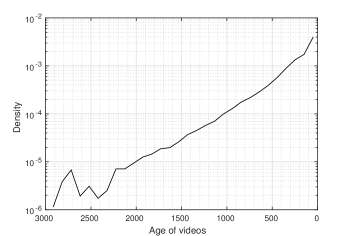
Figure 18: The fraction of videos in the dataset as a function of the age of the videos. There is a significant percentage of newer videos (videos with less age) compared to older videos. Hence, the dataset capture the exponential growth of the number of videos uploaded to YouTube.

Similar to [156], we define three categories of videos based on their popularity: Highly popular, popular, and unpopular. Table 3 gives a summary of the fraction of videos in the dataset belonging to each category. As can be seen from Table 3, the majority of the videos in the dataset belong to the popular category.

Table 3: Popularity distribution of videos in the dataset

Criteria	Fraction
Highly Popular (Total Views $>10^{4}$)	0.12
Popular ($150<$ Total Views $<10^{4}$)	0.67
Unpopular (Total Views $<150$)	0.21

A unique feature of the dataset is that it contains information about the “meta-level optimization” for videos. The meta-level optimization is a change in the title, tags or thumbnail, of an existing video in order to increase the popularity. BBTV markets a product that intelligently automates the meta-level optimization. Table 4 gives a summary of the statistics of the various meta-level optimization present in the dataset.

Table 4: Optimization summary statistics

Optimization	# Videos
Title change	$21$ thousand
Thumbnail change	$13$ thousand
Keyword change	$21$ thousand

5.2 Social Sensor Engagement Sensitivity to Meta-Level Optimization

Here we analyze how changing meta-level features, after a video is posted, impacts the user engagement of the video. Meta-level data plays a significant role in the discovery of content, through YouTube search, and in video recommendation, through the YouTube related videos. Hence, “optimizing” the meta-level data to enhance the discoverability and user engagement of videos is of significant importance to content providers. Therefore, in this section, we study how optimizing the title, thumbnail or keywords affect the view count of YouTube videos.

To perform the sensitivity analysis we utilize the dataset presented in Sec.5.1, and remove any time-sensitive videos. Time-sensitive videos are those videos that are relevant for a short period of time and the popularity of such videos cannot be improved by optimization. We removed the following two time-sensitive categories of videos: “politics” and “movies and trailers”. In addition, we removed videos (from other categories) which contained the following keywords in their video meta-data: “holiday”, “movie”, or “trailers”. For example, holiday videos are not watched frequently during off-holiday times.

Let $\hat{\tau}_{i}$ be the time at which the meta-level optimization was performed on video $i$ and let $s_{i}$, denote the corresponding sensitivity. We characterize the sensitivity to meta-level optimization as follows:

$$s_{i}=\frac{\left(\sum_{t=\hat{\tau}_{i}}^{\hat{\tau}_{i}+6}v_{i}(t)\right)/7}{\left(\sum_{t=\hat{\tau}_{i}-6}^{\hat{\tau}_{i}}v_{i}(t)\right)/7}$$ (60)

The numerator of (60) is the mean value of the view count $7$ days after optimization. Similarly, the denominator of (60) is the mean value of the view count $7$ days before optimization. The results are provided in Table 5 for optimization of the title, thumbnail, and keywords.

Optimization	Fraction of Videos with increased popularity
Title change	0.52
Thumbnail change	0.533
Keyword change	0.50
No change	0.35

Table 5: Sensitivity to Meta-Level Optimization. The table shows than in more than $50\%$ the videos, meta-level optimization resulted in an increase in the popularity of the video.

As shown in Table 5, at least half of the optimizations resulted in an increase in the popularity of the video. In addition, compared to videos with no optimization, the meta-level optimization improves the probability of increased popularity by $45\%$. This is consistent with YouTube and BBTV recommendation to optimize meta-level features to increase user engagement. However, some class of videos benefit from optimizing meta-data much more than others. The effect may be due to small user channels, which have limited number of videos and subscribers, gain by optimizing the meta-level data of the video compared to hugely popular channels such as Sony or CNN. The highly popular channel (e.g. Sony or CNN) upload videos frequently (even multiple times daily), so video content becomes irrelevant quickly. The question of which class of users gain by optimizing the meta level features of the video is part of our ongoing research.

Table 6 summarizes the impact of various meta-level changes on the three major sources of YouTube traffic, i.e. YouTube search, YouTube promoted and traffic from related videos. For those videos where meta-level optimization increased the popularity (the ratio of the mean value of the views after and before optimization is higher than one), we computed the sensitivity for various traffic sources as in (60). Table 6 summarizes the median statistics of the ratio of the traffic sources before and after optimization.

Optimization	Related	Promoted	Search
Title change	$1.13$	NA	$\mathbf{1.24}$
Thumbnail change	$\mathbf{1.20}$	NAfoot:data:na	$1.125$
Keyword change	$\mathbf{1.10}$	$\mathbf{1.16}$	$1$

Table 6: Sensitivity of various traffic sources to meta-level optimization, for videos with increased popularity. The title optimization resulted in significant improvement (approximately $25\%$) from the YouTube search. Similarly, thumbnail optimization improved traffic from the related videos and keyword optimization resulted in increased traffic from related and promoted videos.

The title optimization resulted in significant improvement (approximately $25\%$) from the YouTube search. Similarly, thumbnail optimization improved traffic from the related videos and keyword optimization resulted in increased traffic from related and promoted videos.

Summary: This section studied the sensitivity of view count with respect to meta-level optimization. The main finding is that meta-level optimization increased the popularity of video in the majority of cases. In addition, we found that optimizing the title improved traffic from YouTube search. Similarly, thumbnail optimization improved traffic from the related videos and keyword optimization resulted in increased traffic from related and promoted videos.

5.3 Causal Relationship Between Channel Subscribers and Social Sensor Engagement

In this section the goal is to detect if a causal relationship exists between subscriber and viewer counts and how it can be used to estimate the next day subscriber count of a channel. The results are of interest for measuring the popularity of a YouTube channel. Fig. 19 displays the subscriber and view count dynamics of a popular movie trailer channel in YouTube. It is clear from Fig. 19 that the subscribers “spike” with a corresponding “spike” in the view count. In this section we model this causal relationship of the subscribers and view count using the Granger causality test from the econometric literature [71].

The main idea of Granger causality is that if the value(s) of a lagged time-series can be used to predict another time-series, then the lagged time-series is said to “Granger cause” the predicted time-series. To formalize the Granger causality model, let $s^{j}(t)$ denote the number of subscribers to a channel $j$ on day $t$, and $v_{i}^{j}(t)$ the corresponding view count for a video $i$ on channel $j$ on day $t$. The total number of videos in a channel on day $t$ is denoted by $\mathcal{I}(t)$. Define,

$$\hat{v}^{j}(t)=\sum_{i=1}^{\mathcal{I}(t)}v_{i}^{j}(t),$$ (61)

as the total view count of channel $j$ at time $t$. The Granger causality test involves testing if the coefficients $b_{i}$ are non-zero in the following equation which models the relationship between subscribers and view counts:

$$s^{j}(t)=\sum_{k=1}^{n_{s}}a_{k}^{j}s^{j}(t-k)+\sum_{i=k}^{n_{v}}b_{k}^{j}\hat{v}^{j}(t-k)+\varepsilon^{j}(t),$$ (62)

where $\varepsilon^{j}(t)$ represents normal white noise for channel $j$ at time $t$. The parameters $\{a_{i}^{j}\}_{\{i=1,\dots,n_{s}\}}$ and $\{b_{i}^{j}\}_{\{i=1,\dots,n_{v}\}}$ are the coefficients of the AR model in (62) for channel $j$, with $n_{s}$ and $n_{v}$ denoting the lags for the subscriber and view counts time series respectively. If the time-series $\mathcal{D}^{j}=\{s^{j}(t),\hat{v}^{j}(t)\}_{t\in\{1,\dots,T\}}$ of a channel $j$ fits the model (62), then we can test for a causal relationship between subscribers and view count. In equation (62), it is assumed that $|a_{i}|<1$, $|b_{i}|<1$ for stationarity. The causal relationship can be formulated as a hypothesis testing problem as follows:

$$H_{0}:b_{1}=\dots=b_{n_{v}}=0\text{ vs. }H_{1}:\text{Atleast one }b_{i}\neq 0.$$ (63)

The rejection of the null hypothesis, $H_{0}$, implies that there is a causal relationship between subscriber and view counts.

First, we use Box-Ljung test [64] is to evaluate the quality of the model (62) for the given dataset $\mathcal{D}^{j}$. If satisfied, then the Granger causality hypothesis (63) is evaluated using the Wald test [182]. If both hypothesis tests pass then we can conclude that the time series $\mathcal{D}^{j}$ satisfies Granger causality–that is, the previous day subscriber and view count have a causal relationship with the current subscriber count.

A key question prior to performing the Granger causality test is what percentage of videos in the YouTube dataset (Appendix) satisfy the AR model in (62). To perform this analysis we apply the Box-Ljung test with a confidence of 0.95 (p-value = $0.05$). First, we need to select $n_{s}$ and $n_{v}$, the number of lags for the subscribers and view count time series. For $n_{s}=n_{v}=1$, we found that only $20\%$ of the channels satisfy the model (62). When $n_{s}$ and $n_{v}$ are increased to $2$, the number of channels satisfying the model increases to $63\%$. For $n_{s}=n_{v}=3$, we found that $91\%$ of the channels satisfy the model (62), with a confidence of $0.95$ (p-value = $0.05$). Hence, in the below analysis we select $n_{s}=n_{v}=3$. It is intersting to note that the mean value of coefficients $b_{i}$ decrease as $i$ increases indicating that older view counts have less influence on the subscriber count. Similar results also hold for the coefficients $a_{i}$. Hence, as expected, the previous day subscriber count and the previous day view count most influence the current subscriber count.

The next key question is does their exist a causal relationship between the subscriber dynamics and the view count dynamics. This is modeled using the hypothesis in (63). To test (63) we use the Wald test with a confidence of $0.95$ (p-value = $0.05$) and found that approximately $55\%$ of the channels satisfy the hypothesis. For approximately $55\%$ of the channels that satisfy the AR model (62), the view count “Granger causes” the current subscriber count. Interestingly, if different channel categories are accounted for then the percentage of channels that satisfy Granger causality vary widely as illustrated in Table 7. For example, $80\%$ of the Entertainment channels satisfy Granger causality while only $40\%$ of the Food channels satisfy Granger causality. These results illustrate the importance of channel owners to not only maximize their subscriber count, but to also upload new videos or increase the views of old videos to increase their channels popularity (i.e. via increasing their subscriber count). Additionally, from our analysis which illustrates that the view count of a posted video is sensitive to the number of subscribers of the channel, increasing the number of subscribers will also increase the view count of videos that are uploaded by the channel owners.

Category	Fraction
Gaming	0.60
Entertainment	0.80
Food	0.40
Sports	0.67

Table 7: Fraction of channels satisfying the hypothesis: View count “Granger causes” subscriber count, split according to category.

Figure 19: Viewcount and subscribers for the popular movie trailer channel: VISOTrailers. The Granger causality test for view counts “Granger causes” subscriber count is true with a p-value of $5\times 10^{-8}$.

5.4 Video Upload Scheduling and Social Sensor Engagement

Here we investigate how the video upload scheduling dynamics of YouTube channels impacts social sensor engagement. We find the interesting property that for popular gaming YouTube channels with a dominant (constant) upload schedule, deviating from the schedule increases the views and the comment counts of the channel (e.g. increases user engagement).

Creator Academy in their best practice section recommends to upload videos on a regular schedule to get repeat views. The reason for a regular upload schedule is to increase the user engagement and to rank higher in the YouTube recommendation list. However, we show in this section that going “off the schedule” can be beneficial for a gaming YouTube channel, with a regular upload schedule, in terms of the number of views and the number of comments.

From the dataset, we “filtered out” video channels with a dominant upload schedules, as follows: The dominant upload schedule was identified by taking the periodogram of the upload times of the channel and then comparing the highest value to the next highest value. If the ratio defined above is greater than $2$, we say that the channel has a dominant upload schedule. From the dataset containing $25$ thousand channels, only $6500$ channels contain a dominant upload schedule. Some channels, particularly those that contain high amounts of copied videos such as trailers, movie/TV snippets upload videos on a daily basis. These have been removed from the above analysis. The expectation is that by doing so we concentrate on those channels that contain only user generated content.

We found that channels with gaming content account for $75\%$ of the $6500$ channels with a dominant upload schedule and the main tags associated with the videos were: “game”, “gameplay” and “videogame”. We computed the average views when the channel goes off the schedule and found that on an average when the channel goes off schedule the channel gains views $97\%$ of the time and the channel gains comments $68\%$ of the time. This suggests that channels with “gameplay” content have periodic upload schedule and benefit from going off the schedule.

5.5 Social Sensor Engagement Dynamics with YouTube Videos

Several time-series analysis methods have been employed in the literature to model the view count dynamics of YouTube videos. These include ARMA time series models [75], multivariate linear regression models [153], hidden Markov models [95], normal distribution fitting [60], and parametric model fitting [156, 157]. Though all these models provide an estimate of the view count dynamics of videos, we are interested in segmenting view count dynamics of a video resulting from subscribers, non-subscribers and exogenous events. Exogenous events are due to video promotion on other social networking platform such as Facebook or the video being referenced by a popular news organization or celebrity on Twitter. Detecting and accounting for exogenous events is motivated by the need for extracting accurate view counts resulting from exogenous events that provide an estimate of the efficiency of video promotion methods and meta-level feature optimizations.

The view count dynamics of popular videos in YouTube typically show an initial viral behaviour, due to subscribers watching the content, and then a linear growth resulting from non-subscribers. The linear growth is due to new users migrating from other channels or due to interested users discovering the content either through search or recommendations (we call this phenomenon migration similar to [156]). Hence, without exogenous events, the view count dynamics of a video due to subscribers and non-subscribers can be estimated using piecewise linear and non-linear segments. In [156], it is shown that a Gompertz time series model can be modeled the view count dynamics from subscribers and non-subscribers, if no exogenous events are present. In this chapter, we generalize the model in [156] to account for views from exogenous events. It should be noted that classical change-point detection methods [170] cannot be used here as the underlying distribution generating the view count is unknown.

To account for the view count dynamics introduced from exogenous events we use the generalized Gompertz model given by:

$$\begin{aligned} \bar{v}_{i}(t)&=\sum_{k=0}^{K_{\text{max}}}w^{k}_{i}(t)u(t-t_{k}),\\ w_{i}^{k}(t)&=M_{k}\left(1-e^{-\eta_{k}\left(e^{b_{k}\left(t-t_{k}\right)}-1\right)}\right)+c_{k}(t-t_{k}),\end{aligned}$$ (64)

where $\bar{v}_{i}(t)$ is the total view count for video $i$ at time $t$, $u(\cdot)$ is the unit step function, $t_{0}$ is the time the video was uploaded, $t_{k}$ with $k\in\{1,\dots,K_{\text{max}}\}$ are the times associated with the $K_{\text{max}}$ exogenous events, and $w^{k}_{i}(t)$ are Gompertz models which account for the view count dynamics from uploading the video and from the exogenous events. In total there are $K_{\text{max}}+1$ Gompertz models with each having parameters $t_{k},M_{k},\eta_{k},b_{k}$. $M_{k}$ is the maximum number of requests not including migration for an exogenous event at $t_{k}$, $\eta_{k}$ and $b_{k}$ model the initial growth dynamics from event $t_{k}$, and $c_{k}$ accounts for the migration of other users to the video. In (64) the parameters $\{M_{k},\eta_{k},b_{k}\}_{k=0}$ are associated with the subscriber views when the video is initially posted, the parameters $\{t_{k},M_{k},\eta_{k},b_{k}\}_{k=1}^{K_{\text{max}}}$ are associated with views introduced from exogenous events, and the views introduced from migration are given by $\{c_{k}\}_{k=0}^{K_{\text{max}}}$. Each Gompertz model (64) captures the initial viral growth when the video is initially available to users, followed by a linearly increasing growth resulting from user migration to the video.

The parameters $\theta_{i}=\{a_{k},t_{k},M_{k},\eta_{k},b_{k},c_{k}\}_{k=0}^{K_{\text{max}}}$ in (64) can be estimated by solving the following mixed-integer non-linear program:

$$\theta_{i} \in\operatorname{arg\ min}\Big{\{}\sum_{t=0}^{T_{i}}\big{(}\bar{v}_{i}(t)-v_{i}(t)\big{)}^{2}+\lambda K\Big{\}}$$

$$K=\sum_{k=0}^{K_{\text{max}}}a_{k},\quad\quad a_{k}\in\{0,1\}\quad\quad k\in\{0,\dots,K_{\text{max}}\},$$ (65)

with $T_{i}$ the time index of the last recorded views of video $v_{i}$, and $a_{k}$ a binary variable equal to $1$ if an exogenous event is present at $t_{k}$. Note that (65) is a difficult optimization problem as the objective is non-convex as a result of the binary variables $a_{k}$ [33]. In the YouTube social network when an exogenous event occurs this causes a large and sudden increase in the number of views, however as seen in Fig. 20, a few days after the exogenous event occurs the views only result from migration (i.e. linear increase in total views). Assuming that each exogenous event is followed by a linear increase in views we can estimate the total number of exogenous events $K_{\text{max}}$ present in a given time-series by first using a segmented linear regression method, and then counting the number of segments of connected linear segments with a slope less then $c_{\text{max}}$. The parameter $c_{\text{max}}$ is the maximum slope for the views to be considered to result from viewer migration. Plugging $K_{\text{max}}$ into (65) results in the optimization of a non-linear program for the unknowns $\{t_{k},M_{k},\eta_{k},b_{k},c_{k}\}_{k=0}^{K_{\text{max}}}$. This optimization problem can be solved using sequential quadratic programming techniques [23].

To illustrate how the Gompertz model (64) can be used to detect for exogenous events, we apply (64) to the view count dynamics of a video that only contains a single exogenous event. Fig. 20 displays the total view count of a video where an exogenous event occurs at time $t=41$ (i.e. $t_{1}=41$ in (64)) days after the video is posted. The initial increase in views for the video for $t\leq 7$ days results from the $2910$ subscribers of the channel viewing the video. For $7\leq t\leq 41$, other users that are not subscribed to the channel migrate to view the video at an approximately constant rate of $13$ views/day. At $t=41$, an exogenous event occurs causing an increase in the views per day. The difference in viewers, resulting from the exogenous event, is $7174$. For $t\geq 43$, the views result primarily from the migration of users to approximately $2$ views/day. Hence, using the generalized Gompertz model (64) we can differentiate between subscriber views, views caused by exogenous events, and views caused by migration.

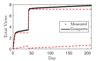
Figure 20: Due to an exogenous event on day $41$, there is a sudden increase in the number of views. The total view count fitted by the Gompertz model $\bar{v}_{i}(t)$ in (64) is shown in black with the virality (exponential) and migration (linear) illustrated by the dotted red.

5.6 Social Sensor Engagement for Channel Playthroughs

One of the most popular sequences of YouTube videos is the video game “playthrough”. A video game playthrough is a set of videos for which each video has a relaxed and casual focus on the game that is being played and typically contains commentary from the user presenting the playthrough. Unlike YouTube channels such as CNN, BBC, and CBC in which each new video can be considered independent from the others, in a video playthrough the future view count of videos are influenced by the previously posted videos in the playthrough. To illustrate this effect we consider a video playthrough for the game “BioShock Infinite”–a popular video game released in 2013. The channel, popular for hosting such video playthroughs, contains close to $4500$ videos and $180$ video playthroughs. The channel is highly popular and has garnered a combined view count close to $100$ million views with $150$ thousand subscribers over a period of $3$ years. Fig. 21 illustrates that the early view count dynamics are highly correlated with the view count dynamics of future videos. Both the short term view count and long term migration of future videos in the playthrough decrease after the initial video in the playthrough is posted. This results for two reasons, either the viewers purchase the game, or the viewers leave as the subsequent playthroughs become repetitive as a result of game quality or video commentary quality. A unique effect with video playthroughs is that although the number of subscribers to the channel hosting the videos in Fig. 21 increases over the 600 day period, the linear migration is still maintained after the initial 50 days after the playthrough is published. Additionally, the slope of the migration is related to the early total view count as illustrated in Fig. 21(b).

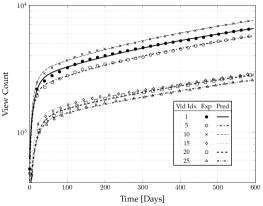
(a) Actual and predicted view count of playthrough. We plot the 1, 5, 10, 15, 20 and 25 video from the playlist containing $25$ videos. In the legend, Exp and Pred corresponds to the actual and the predicted value using (64), respectively. Figure shows that the view counts decreases for subsequent videos in the playlist.

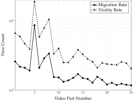
(b) The virality rate specifies the early views due to subscribers, and the migration rate (in units of views/1000 days) specifies the subsequent linear growth due to non-subscribers.

Figure 21: Actual and predicted view count of a playthrough containing 25 YouTube videos for the game “BioShock Infinite”. The predictions are computed by fitting a modified Gompertz model (64) to the measured view count for each video in the playthrough.

5.7 Summary and Extensions

The application of time-series analysis and machine learning methods to gain insight into the social sensor dynamics on YouTube is an active area of research with several promising outcomes. First, they can be used to reduce the operating cost of content distribution networks. In [88] a two time-scale game-theoretic learning algorithm is constructed to optimally cache videos in the future 5G mobile network based on the dynamics of the social sensors. In [164] the optimal caching decision is formulated as a mixed-integer linear program that accounts for the dynamics of the social sensors. Second, knowledge of the user dynamics can be used to optimize the meta-level features of videos to maximize user engagement as illustrated in this section.

Significant work remains on the analysis of user dynamics in the YouTube social network. Recall that in the YouTube social network interaction between users and channel owners include:

1. Commenting on users videos. Commenting is YouTube’s version of engagement, and it has some of the most involved, engaged and dedicated users. Additionally, users can comment on other users comments which is very similar to users interaction on blog posting sites except related to the uploaded videos.

2. Subscribing to YouTube channels provides a method of forming relationships between users.

3. Users can directly comment on a YouTube channel without the need to only interact when a video is posted.

4. Users can also interact by embedding videos from another users channel directly into their own channel to promote exposure or form communities of users.

In addition to the social incentives, YouTube provides monetary incentives to promote users increasing their popularity and engagement. As more users view and interact with a users video or channel, YouTube will pay the user proportional to the advertisement exposure on the users channel. Therefore, users not only maximize exposure to increase their social popularity, but also for monetary gain which introduces unique dynamics in the formation of edges in the YouTube social network. Using the dataset discussed in Sec.5.1, Fig.22 plots the communication network where an edge indicates comments and responses between users that have interacted at least 1000 times. From Fig.22(a), initially there appears to be two clusters of users that have strong interactions indicating that user preferences play a significant role in forming the edges in these clusters. After a period of 3 months, Fig.22(b) illustrates that more users have entered the network however there still appears to be two primary clusters of interacting users. At 6 months, Fig.22(c) shows a dense interaction between several users in the social network. The dynamics of these interaction links are governed by both the users preferences and the video content that is uploaded by the users. Prior to edge formation, these clustered communities can detected by applying the homophilic community detection tests introduced in [66]. These tests are designed to cluster users based on their content preferences.

The dynamics of edge formation/destruction and user popularity in the social network (illustrated in Fig.22) are governed by the user-user interaction and the user-content-user interaction. Two key question to address in the YouTube social network is: How do the social dynamics (subscribing, commenting, video content quality, video category, etc.) impact the popularity of videos and the dynamics of the communication network between users? Answers to this question provides valuable insight into the evolving dynamics of the social network illustrated in Fig.22.

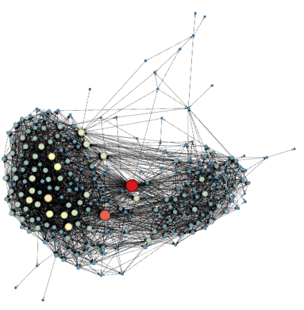
(a) Initial: 239 users, 3,112 edges.

(b) After 3 months: 503 users, 8,558 edges.

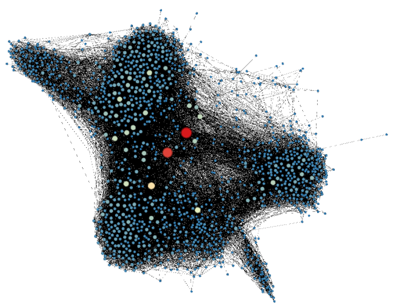
(c) After 6 months: 1,391 users, 31,701 edges.

Figure 22: Snapshots of the YouTube social network at 0 months, 3 months, and 6 months constructed using the dataset discussed in Sec.5.1. Node sizes and color indicate their degree (red is higher, blue is lower). The complete social network is composed of over 1.13 million users, and contains over 2.98 million edges. Only users with at least 1000 edges are displayed.

6 Closing Remarks

This chapter has discussed four important and inter-related themes regarding the dynamics of social sensors, namely, diffusion models for information in social networks, Bayesian social learning, revealed preferences and how social sensors interact over YouTube channels. In each case, examples involving real datasets were given to illustrate the various concepts. The unifying theme behind these three topics stems from predicting global behavior given local behavior: individual social sensors make decisions and learn from other social sensors and we are interested in understanding the behavior of the entire network. In Sec.2 we showed that the global degree of infected nodes can be determined by mean field dynamics. In Sec.3, it was shown that despite the apparent simplicity in information flows between social sensors, the global system can exhibit unusual behavior such as herding and data incest. Finally, in Sec.4 a non-parametric method was used to determine the utility functions of a multiagent system - this can be used to predict the response of the system.

This chapter has dealt with social sensing issues of relevance to a signal processing audience. There are several topics of relevance to social sensors that are omitted due to space constraints, including:

• Coordination of decisions via game-theoretic learning [79, 80, 141] or Bayesian game models such as global games [12]

• Consensus formation over social networks and cooperative models of network formation [103, 169]

• Controlled information fusion in social learning [24].

• Small world models [183, 100]

• Peer to peer media sharing [76, 189]

• Privacy and security modelling [116, 126]

• Influence Maximization; see [142] are references therein.

• Polling using friendship paradox; see [143] are references therein.

• The mobile edge cloud and popularity prediction for YouTube [90].

References

- [1] D. Acemoglu, M. Dahleh, I. Lobel, and A. Ozdaglar. Bayesian learning in social networks. Working Paper 14040, National Bureau of Economic Research, May 2008.
- [2] D. Acemoglu and A. Ozdaglar. Opinion dynamics and learning in social networks. Dynamic Games and Applications, 1(1):3–49, 2011.
- [3] H. Achrekar, A. Gandhe, R. Lazarus, S. Yu, and B. Liu. Predicting flu trends using twitter data. In 2011 IEEE Conference on Computer Communications Workshops, pages 702–707. IEEE, 2011.
- [4] H. Achrekar, A. Gandhe, R. Lazarus, S. Yu, and B. Liu. Twitter improves seasonal influenza prediction. In HEALTHINF 2012 International Conference on Health Informatics, pages 61–70, 2012.
- [5] A. Adams, R. Blundell, M. Browning, and I. Crawford. Prices versus preferences: taste change and revealed preference. Technical report, IFS Working Papers, 2015.
- [6] G. Adomavicius and A. Tuzhilin. Toward the next generation of recommender systems: A survey of the state-of-the-art and possible extensions. IEEE Transactions on Knowledge and Data Engineering, 17(6):734–749, 2005.
- [7] S. Afriat. The construction of utility functions from expenditure data. International economic review, 8(1):67–77, 1967.
- [8] S. Afriat. Logic of choice and economic theory. Clarendon Press Oxford, 1987.
- [9] D. Aldous. Interacting particle systems as stochastic social dynamics. Bernoulli, 19(4):1122–1149, 2013.
- [10] R. Amir. Supermodularity and complementarity in economics: An elementary survey. Southern Economic Journal, 71(3):636–660, 2005.
- [11] C. Anderson and G. J. Kilduff. Why do dominant personalities attain influence in face-to-face groups? the competence-signaling effects of trait dominance. Journal of Personality and Social Psychology, 96(2):491–503, 2009.
- [12] G. Angeletos, C. Hellwig, and A. Pavan. Dynamic global games of regime change: Learning, multiplicity, and the timing of attacks. Econometrica, 75(3):711–756, 2007.
- [13] A. Aprem and V. Krishnamurthy. Utility change point detection in online social media: A revealed preference framework. IEEE Transactions on Signal Processing, 65(7):1869–1880, 2017.
- [14] P. Artzner, F. Delbaen, J.-M. Eber, and D. Heath. Coherent measures of risk. Risk Management: Value at Rrisk and Beyond, page 145, 2002.
- [15] S. Asur and B. A. Huberman. Predicting the future with social media. In 2010 IEEE/WIC/ACM International Conference on Web Intelligence and Intelligent Agent Technology (WI-IAT), volume 1, pages 492–499. IEEE, 2010.
- [16] R. J. Aumann. Agreeing to disagree. The Annals of Statistics, 4(6):1236–1239, Nov. 1976.
- [17] M. Babaioff, R. Kleinberg, and C. Papadimitriou. Congestion games with malicious players. In Proceedings of the 8th ACM Conference on Electronic Commerce, EC ’07, pages 103–112, New York, NY, USA, 2007. ACM.
- [18] A. Banerjee. A simple model of herd behavior. Quaterly Journal of Economics, 107(3):797–817, August 1992.
- [19] A. Barabasi and A. Reka. Emergence of scaling in random networks. Science, 286(5439):509, 1999.
- [20] E. Beigman and R. Vohra. Learning from revealed preference. In Proceedings of the 7th ACM Conference on Electronic Commerce, EC ’06, pages 36–42, New York, NY, USA, 2006. ACM.
- [21] M. Benaïm and J. Weibull. Deterministic approximation of stochastic evolution in games. Econometrica, 71(3):873–903, 2003.
- [22] A. Benveniste, M. Metivier, and P. Priouret. Adaptive Algorithms and Stochastic Approximations, volume 22 of Applications of Mathematics. Springer-Verlag, 1990.
- [23] D. P. Bertsekas. Nonlinear programming. Athena scientific, 1999.
- [24] S. Bhatt and V. Krishnamurthy. Controlled information fusion with risk-averse cvar social sensors. arXiv preprint arXiv:1712.07773, 2017.
- [25] S. Bikchandani, D. Hirshleifer, and I. Welch. A theory of fads, fashion, custom, and cultural change as information cascades. Journal of Political Economy, 100(5):992–1026, October 1992.
- [26] R. Blundell. How revealing is revealed preference? Journal of the European Economic Association, 3(2-3):211–235, 2005.
- [27] J. Bollen, H. Mao, and X. Zeng. Twitter mood predicts the stock market. Journal of Computational Science, 2(1):1–8, 2011.
- [28] R. Bond, C. Fariss, J. Jones, A. Kramer, C. Marlow, J. Settle, and J. Fowler. A 61-million-person experiment in social influence and political mobilization. Nature, 489:295–298, September 2012.
- [29] V. Borkar and P. Varaiya. Asymptotic agreement in distributed estimation. IEEE Transactions on Automatic Control, 27(3):650–655, 1982.
- [30] S. Borle, P. Boatwright, and J. Kadane. The timing of bid placement and extent of multiple bidding: An empirical investigation using ebay online auctions. Statistical Science, pages 194–205, 2006.
- [31] S. Boyd and L. Vandenberghe. Convex Optimization. Cambridge University Press, 2004.
- [32] D. Broniatowski, M. Paul, and M. Dredze. National and local influenza surveillance through twitter: An analysis of the 2012-2013 influenza epidemic. PloS one, 8(12):e83672, 2013.
- [33] S. Burer and A. Letchford. Non-convex mixed-integer nonlinear programming: a survey. Surveys in Operations Research and Management Science, 17(2):97–106, 2012.
- [34] A. Cartea and S. Jaimungal. Modelling asset prices for algorithmic and high-frequency trading. Applied Mathematical Finance, 20(6):512–547, 2013.
- [35] A. Carvajal, R. Deb, J. Fenske, and J. Quah. Revealed preference tests of the cournot model. Econometrica, 81(6):2351–2379, 2013.
- [36] C. Chamley. Rational herds: Economic Models of Social Learning. Cambridge University Press, 2004.
- [37] C. Chamley, A. Scaglione, and L. Li. Models for the diffusion of beliefs in social networks: An overview. IEEE Signal Processing Magazine, 30(3):16–29, 2013.
- [38] A. Chapman, G. Verbic, and D. Hill. A healthy dose of reality for game-theoretic approaches to residential demand response. In 2013 IREP Symposium Bulk Power System Dynamics and Control-IX Optimization, Security and Control of the Emerging Power Grid (IREP), pages 1–13. IEEE, 2013.
- [39] G. C. Chasparis and J. S. Shamma. Control of preferences in social networks. In Decision and Control (CDC), 2010 49th IEEE Conference on, pages 6651–6656. IEEE, 2010.
- [40] K. C. Chen, M. Chuang, and H. V. Poor. From technological networks to social networks. IEEE Journal on Selected Areas Communications, 31(9):548–572, Sept. 2013.
- [41] N. Chen. On the approximability of influence in social networks. SIAM Journal on Discrete Mathematics, 23(3):1400–1415, 2009.
- [42] Z. Cheng, J. Caverlee, and K. Lee. You are where you tweet: A content-based approach to geo-locating Twitter users. In Proceedings of the 19th ACM International Conference on Information and Knowledge Management, pages 759–768. ACM, 2010.
- [43] N. Christakis and J. Fowler. Social network sensors for early detection of contagious outbreaks. PloS one, 5(9):e12948, 2010.
- [44] R. A. Cohn, W. G. Lewellen, R. C. Lease, and G. G. Schlarbaum. Individual investor risk aversion and investment portfolio composition. The Journal of Finance, 30(2):605–620, 1975.
- [45] T. Cover and M. Hellman. The two-armed-bandit problem with time-invariant finite memory. IEEE Transactions on Information Theory, 16(2):185–195, 1970.
- [46] A. Culotta. Towards detecting influenza epidemics by analyzing twitter messages. In Proceedings of the first workshop on social media analytics, pages 115–122. ACM, 2010.
- [47] A. Culotta. Lightweight methods to estimate influenza rates and alcohol sales volume from twitter messages. Language resources and evaluation, 47(1):217–238, 2013.
- [48] A. Culotta. Lightweight methods to estimate influenza rates and alcohol sales volume from twitter messages. Language resources and evaluation, 47(1):217–238, 2013.
- [49] A. Dasgupta, R. Kumar, and D. Sivakumar. Social sampling. In Proceedings of the 18th ACM SIGKDD international conference on Knowledge discovery and data mining, pages 235–243, Beijing, 2012. ACM.
- [50] S. Dave, M. Sooriyabandara, and L. Zhang. Application of a game-theoretic energy management algorithm in a hybrid predictive-adaptive scenario. In 2011 2nd IEEE PES International Conference and Exhibition on Innovative Smart Grid Technologies (ISGT Europe), pages 1–6, 2011.
- [51] R. Deb. Interdependent preferences, potential games and household consumption. MPRA Paper 6818, University Library of Munich, Germany, Jan 2008.
- [52] R. Deb. A testable model of consumption with externalities. Journal of Economic Theory, 144(4):1804 – 1816, 2009.
- [53] S. DellaVigna. Psychology and economics: Evidence from the field. Journal of Economic Literature, 47(2):315–72, 2009.
- [54] W. Diewert. Afriat and revealed preference theory. The Review of Economic Studies, pages 419–425, 1973.
- [55] B. Donkers and A. V. Soest. Subjective measures of household preferences and financial decisions. Journal of Economic Psychology, 20(6):613 – 642, 1999.
- [56] A. Doucet, N. Gordon, and V. Krishnamurthy. Particle filters for state estimation of jump Markov linear systems. IEEE Transactions on Signal Processing, 49:613–624, 2001.
- [57] D. Easley and J. Kleinberg. Networks, Crowds, and Markets: Reasoning About a Highly Connected World. Cambridge University Press, 2010.
- [58] R. Elliott, L. Aggoun, and J. Moore. Hidden Markov Models – Estimation and Control. Springer-Verlag, New York, 1995.
- [59] P. Erdös and A. Rényi. On random graphs, I. Publicationes Mathematicae (Debrecen), 6:290–297, 1959.
- [60] F. Figueiredo, F. Benevenuto, and J. Almeida. The tube over time: characterizing popularity growth of youtube videos. In Proceedings of the fourth ACM international conference on Web search and data mining, pages 745–754. ACM, 2011.
- [61] F. Forges and E. Minelli. Afriat’s theorem for general budget sets. Journal of Economic Theory, 144(1):135–145, 2009.
- [62] A. Fostel, H. Scarf, and M. Todd. Two new proofs of Afriat’s theorem. Economic Theory, 24(1):211–219, 2004.
- [63] D. Fudenberg, R. Iijima, and T. Strzalecki. Stochastic choice and revealed perturbed utility. Econometrica, 83(6):2371–2409, 2015.
- [64] G. E. P. B. G. M. Ljung. On a measure of lack of fit in time series models. Biometrika, 65(2):297–303, 1978.
- [65] J. Geanakoplos and H. Polemarchakis. We can’t disagree forever. Journal of Economic Theory, 28(1):192 – 200, 1982.
- [66] O. Gharehshiran, W. Hoiles, and V. Krishnamurthy. Detection of homophilic communities and coordination of interacting meta-agents: A game-theoretic viewpoint. IEEE Transactions on Signal and Information Processing over Networks, 2(1):84–101, 2016.
- [67] G. Ghoshal, L. Chi, and A.-L. Barabási. Uncovering the role of elementary processes in network evolution. Scientific Reports, 3:2920, 2013.
- [68] F. Giummolè, S. Orlando, and G. Tolomei. A study on microblog and search engine user behaviors: How twitter trending topics help predict google hot queries. HUMAN, 2(3):195, 2013.
- [69] S. Goel and M. J. Salganik. Respondent-driven sampling as Markov chain Monte Carlo. Statistics in Medicine, 28:2209–2229, 2009.
- [70] S. Goel, D. Watts, and D. Goldstein. The structure of online diffusion networks. In Proceedings of the 13th ACM conference on Electronic Commerce, pages 623–638. ACM, 2012.
- [71] C. W. Granger. Investigating causal relations by econometric models and cross-spectral methods. Econometrica: Journal of the Econometric Society, pages 424–438, 1969.
- [72] M. Granovetter. Threshold models of collective behavior. American Journal of Sociology, 83(6):1420–1443, May 1978.
- [73] M. Granovetter. Economic action and social structure: the problem of embeddedness. American journal of sociology, pages 481–510, 1985.
- [74] M. Granovetter. The impact of social structure on economic outcomes. Journal of economic perspectives, pages 33–50, 2005.
- [75] G. Gürsun, M. Crovella, and I. Matta. Describing and forecasting video access patterns. In 2011 Proc. of INFOCOM, pages 16–20. IEEE, 2011.
- [76] M. J. Halvey and M. T. Keane. Exploring social dynamics in online media sharing. In Proceedings of 16th international conference on World Wide Web, pages 1273–1274, Banff, AB, Canada, May 2007.
- [77] M. Hamdi and V. Krishnamurthy. Removal of Data Incest in Multi-agent Social Learning in Social Networks. ArXiv e-prints, Sept. 2013.
- [78] M. Hamdi, V. Krishnamurthy, and G. Yin. Tracking a Markov-modulated stationary degree distribution of a dynamic random graph. IEEE Transactions on Information Theory, 60(10):6609–6625, 2014.
- [79] S. Hart and A. Mas-Colell. A simple adaptive procedure leading to correlated equilibrium. Econometrica, 68(5):1127–1150, 1 2000.
- [80] S. Hart, A. Mas-Colell, and Y. Babichenko. Simple Adaptive Strategies: From Regret-Matching to Uncoupled Dynamics, volume 4 of World Scientific Series in Economic Theory. World Scientific Publishing, 2013.
- [81] A. Hayrapetyan, E. Tardos, and T. Wexler. The effect of collusion in congestion games. In Proceedings of the Thirty-eighth Annual ACM Symposium on Theory of Computing, STOC ’06, pages 89–98. ACM, 2006.
- [82] D. D. Heckathorn. Respondent-driven sampling: a new approach to the study of hidden populations. Social Problems, 44:174–199, 1997.
- [83] D. D. Heckathorn. Respondent-driven sampling ii: deriving valid population estimates from chain-referral samples of hidden populations. Social Problems, 49:11–34, 2002.
- [84] M. Hellman and T. Cover. Learning with finite memory. The Annals of Mathematical Statistics, 41(3):765–782, 1970.
- [85] M. Hernández-González and M. V. Basin. Discrete-time filtering for nonlinear polynomial systems over linear observations. International Journal of Systems Science, 45(7):1461–1472, 2014.
- [86] H. W. Hethcote. The mathematics of infectious diseases. SIAM Review, 42(4):599–653, 2000.
- [87] W. Hoiles, A. Aprem, and V. Krishnamurthy. Engagement and popularity dynamics of youtube videos and sensitivity to meta-data. IEEE Transactions on Knowledge & Data Engineering, 7:1426–1437, 2017.
- [88] W. Hoiles, O. N. Gharehshiran, V. Krishnamurthy, N.-D. Ðào, and H. Zhang. Adaptive caching in the youtube content distribution network: A revealed preference game-theoretic learning approach. IEEE Transactions on Cognitive Communications and Networking, 1(1):71–85, 2015.
- [89] W. Hoiles and V. Krishnamurthy. Nonparametric demand forecasting and detection of demand-responsive consumers. IEEE Transactions on Smart Grid, 6(2):695–704, 2015.
- [90] W. Hoiles, S. S. Tanzil, and V. Krishnamurthy. Risk-averse caching policies for youtube content in femtocell networks using density forecasting. IEEE Transactions on Cloud Computing, 2018.
- [91] C. Ibars, M. Navarro, and L. Giupponi. Distributed demand management in smart grid with a congestion game. In 2010 First IEEE International Conference on Smart Grid Communications, pages 495–500. IEEE, 2010.
- [92] B. Ifrach, C. Maglaras, and M. Scarsini. Monopoly pricing in the presence of social learning. NET Institute Working Paper No. 12-01, 2011.
- [93] M. Jackson. Social and Economic Networks. Princeton University Press, 2010.
- [94] M. O. Jackson and B. W. Rogers. Relating network structure to diffusion properties through stochastic dominance. The BE Journal of Theoretical Economics, 7(1), 2007.
- [95] L. Jiang, Y. Miao, Y. Yang, Z. Lan, and A. Hauptmann. Viral video style: a closer look at viral videos on YouTube. In Proceedings of International Conference on Multimedia Retrieval, page 193. ACM, 2014.
- [96] Y. Kanoria and O. Tamuz. Tractable Bayesian social learning on trees. In Proceedings of the IEEE International Symposium on Information Theory (ISIT), pages 2721 –2725, Jul. 2012.
- [97] S. Karlin. Total Positivity, volume 1. Stanford Univ., 1968.
- [98] S. Karlin and Y. Rinott. Classes of orderings of measures and related correlation inequalities. I. Multivariate totally positive distributions. Journal of Multivariate Analysis, 10(4):467–498, December 1980.
- [99] D. Kempe, J. Kleinberg, and E. Tardos. Maximizing the spread of influence through a social network. In Proceedings of the 9th ACM SIGKDD International Conference on Knowledge Discovery and Data Mining, pages 137–146, Washington, DC, Aug 2003.
- [100] J. Kleinberg. Navigation in a small world. Nature, 406(6798):845–845, Aug. 2000.
- [101] J. Kleinberg and P. Raghavan. Query incentive networks. In 46th Annual IEEE Symposium onFoundations of Computer Science, 2005. FOCS 2005., pages 132–141. IEEE, 2005.
- [102] I. Konstas, V. Stathopoulos, and J. M. Jose. On social networks and collaborative recommendation. In Proceedings of the 32nd International ACM SIGIR conference on Research and Development in Information Retrieval, pages 195–202. ACM, 2009.
- [103] B. Kozma and A. Barrat. Consensus formation on adaptive networks. Physical Review E, 77(1):016102, 2008.
- [104] V. Krishnamurthy. Bayesian sequential detection with phase-distributed change time and nonlinear penalty - A POMDP lattice programming approach. IEEE Transactions on Information Theory, 57(10):7096–7124, 2011.
- [105] V. Krishnamurthy. Quickest detection POMDPs with social learning: Interaction of local and global decision makers. IEEE Transactions on Information Theory, 58(8):5563–5587, 2012.
- [106] V. Krishnamurthy. Partially Observed Markov Decision Processes. Cambridge University Press, 2016.
- [107] V. Krishnamurthy and S. Bhatt. Sequential detection of market shocks with risk-averse cvar social sensors. IEEE Journal of Selected Topics in Signal Processing, 10(6):1061–1072, 2016.
- [108] V. Krishnamurthy, S. Bhatt, and T. Pedersen. Tracking infection diffusion in social networks: Filtering algorithms and threshold bounds. IEEE Transactions on Signal and Information Processing over Networks, 2017.
- [109] V. Krishnamurthy, O. N. Gharehshiran, and M. Hamdi. Interactive sensing and decision making in social networks. Foundations and Trends® in Signal Processing, 7(1-2):1–196, 2014.
- [110] V. Krishnamurthy and M. Hamdi. Mis-information removal in social networks: Dynamic constrained estimation on directed acyclic graphs. IEEE Journal Selected Topics in Signal Processing, 7(2):333–346, May 2013.
- [111] V. Krishnamurthy and W. Hoiles. Afriat’s test for detecting malicious agents. IEEE Signal Processing Letters, 19(12):801–804, 2012.
- [112] V. Krishnamurthy and H. V. Poor. Social learning and Bayesian games in multiagent signal processing: How do local and global decision makers interact? IEEE Signal Processing Magazine, 30(3):43–57, 2013.
- [113] V. Krishnamurthy and H. V. Poor. A tutorial on interactive sensing in social networks. IEEE Transactions on Computational Social Systems, 1(1):3–21, March 2014.
- [114] H. Kushner and G. Yin. Stochastic Approximation Algorithms and Recursive Algorithms and Applications. Springer-Verlag, 2nd edition, 2003.
- [115] S. Lahaie. Kernel methods for revealed preference analysis. In ECAI 2010: 19th European Conference on Artificial Intelligence, pages 439–444, 2010.
- [116] P. G. Lange. Publicly private and privately public: Social networking on youtube. Journal of Computer-Mediated Communication, 13(1):361–380, Oct. 2007.
- [117] A. Lansky, A. Abdul-Quader, M. Cribbin, T. Hall, T. Finlayson, R. Garffin, L. S. Lin, and P. Sullivan. Developing an HIV behavioral survelillance system for injecting drug users: the National HIV Behavioral Surveillance System. Public Health Reports, 122(S1):48–55, 2007.
- [118] C. Leberknight, H. Inaltekin, M. Chiang, and H. Poor. The evolution of online social networks: A tutorial survey. IEEE Signal Processing Magazine, 29(2):41–52, 2012.
- [119] R. Lee and K. Sumiya. Measuring geographical regularities of crowd behaviors for Twitter-based geo-social event detection. In Proceedings of the 2nd ACM SIGSPATIAL International Workshop on Location Based Social Networks, pages 1–10. ACM, 2010.
- [120] S. Lee. Understanding respondent driven sampling from a total survey error perspective. Survey Practice, 2(6), 2009.
- [121] J. Leskovec. SNAP library. http://snap.stanford.edu/data/index.html.
- [122] J. Leskovec, L. A. Adamic, and B. A. Huberman. The dynamics of viral marketing. ACM Transactions on the Web (TWEB), 1(1):5, 2007.
- [123] J. Leskovec and C. Faloutsos. Sampling from large graphs. In Proceedings of the 12th ACM SIGKDD International Conference on Knowledge Discovery and Data Mining, pages 631–636, Philadelphia, 2006. ACM press.
- [124] J. Li and C. Cardie. Early stage influenza detection from twitter. arXiv preprint arXiv:1309.7340, 2013.
- [125] C. Lim, H. D. Sherali, and S. Uryasev. Portfolio optimization by minimizing conditional value-at-risk via nondifferentiable optimization. Computational Optimization and Applications, 46(3):391–415, 2010.
- [126] L. Liu, E. Yu, and J. Mylopoulos. Security and privacy requirements analysis within a social setting. In Proceedings of 11th IEEE International Requirements Engineering Conference, pages 151–161, Monterey Bay, CA, Sep. 2003.
- [127] I. Lobel, D. Acemoglu, M. Dahleh, and A. Ozdaglar. Preliminary results on social learning with partial observations. In Proceedings of the 2nd International Conference on Performance Evaluation Methodolgies and Tools, page 69, Nantes, France, 2007. ACM.
- [128] A. Logothetis and V. Krishnamurthy. Expectation maximization algorithms for MAP estimation of jump Markov linear systems. IEEE Transactions on Signal Processing, 47(8):2139–2156, August 1999.
- [129] D. López-Pintado. Contagion and coordination in random networks. International Journal of Game Theory, 34(3):371–381, 2006.
- [130] D. López-Pintado. Diffusion in complex social networks. Games and Economic Behavior, 62(2):573–590, 2008.
- [131] M. Luca. Reviews, reputation, and revenue: The case of Yelp.com, Technical Report 12-016. Harvard Business School, September 2011.
- [132] M. Malekinejad, L. Johnston, C. Kendall, L. Kerr, M. Rifkin, and G. Rutherford. Using respondent-driven sampling methodology for HIV biological and behavioral surveillance in international settings: a systematic review. AIDS and Behavior, 12(S1):105–130, 2008.
- [133] A. Mas-Colell. On revealed preference analysis. The Review of Economic Studies, pages 121–131, 1978.
- [134] D. L. McFadden and M. Fosgerau. A theory of the perturbed consumer with general budgets. Technical report, National Bureau of Economic Research, 2012.
- [135] P. McGill and M. Schumaker. Boundary conditions for single-ion diffusion. Biophysical Journal, 71:1723–1742, 1996.
- [136] P. Milgrom. Good news and bad news: Representation theorems and applications. Bell Journal of Economics, 12(2):380–391, 1981.
- [137] P. Milgrom and C. Shannon. Monotone comparative statistics. Econometrica, 62(1):157–180, 1992.
- [138] S. Mitra and T. Ji. Risk measures in quantitative finance. International Journal of Business Continuity and Risk Management, 1(2):125–135, 2010.
- [139] E. Mossel and S. Roch. On the submodularity of influence in social networks. In Proceedings of 39th Annual ACM Symposium on Theory of Computing, pages 128–134. ACM, 2007.
- [140] K. Murphy, Y. Weiss, and M. Jordan. Loopy belief propagation for approximate inference: an empirical study. In Proceedings of the Fifteenth Conference Uncertainty in Artificial Intelligence, pages 467–475, 1999.
- [141] O. Namvar, V. Krishnamurthy, and G. Yin. Distributed tracking of correlated equilibria in regime switching noncooperative games. IEEE Transactions on Automatic Control, 58(10):2435–2450, 2013.
- [142] B. Nettasinghe and V. Krishnamurthy. Influence maximization over markovian graphs: A stochastic optimization approach. IEEE Transactions on Signal and Information Processing over Networks, 2018.
- [143] B. Nettasinghe and V. Krishnamurthy. What do your friends think? efficient polling methods for networks using friendship paradox. arXiv preprint arXiv:1802.06505, 2018.
- [144] M. F. Neuts. Structured stochastic matrices of MG-1 type and their applications. Dekker, 1989.
- [145] A. Neyman. Correlated equilibrium and potential games. Int. J. Game Theory, 26(2):223–227, 1997.
- [146] H. Nguyen, J. Song, and Z. Han. Demand side management to reduce peak-to-average ratio using game theory in smart grid. In 2012 IEEE Conference on Computer Communications Workshops (INFOCOM WKSHPS), pages 91 –96, 2012.
- [147] A. Ockenfels and A. Roth. The timing of bids in internet auctions: Market design, bidder behavior, and artificial agents. AI magazine, 23(3):79, 2002.
- [148] M. Ottaviani and P. Sørensen. Information aggregation in debate: Who should speak first? Journal of Public Economics, 81(3):393–421, 2001.
- [149] J. Palmquist, S. Uryasev, and P. Krokhmal. Portfolio optimization with conditional value-at-risk objective and constraints. Department of Industrial & Systems Engineering, University of Florida, 1999.
- [150] B. Pang and L. Lee. Opinion mining and sentiment analysis. Foundations and Trends in Information Retrieval, 2(1-2):1–135, 2008.
- [151] R. Pastor-Satorras and A. Vespignani. Epidemic spreading in scale-free networks. Physical Review Letters, 86(14):3200, 2001.
- [152] J. Pearl. Fusion, propagation, and structuring in belief networks. Artificial Intelligence, 29(3):241 – 288, 1986.
- [153] H. Pinto, J. Almeida, and M. GonXcalves. Using early view patterns to predict the popularity of YouTube videos. In Proc. of the sixth ACM Int. Conf. on Web search and Data mining, pages 365–374. ACM, 2013.
- [154] M. A. Porter and J. P. Gleeson. Dynamical systems on networks: A tutorial, volume 4. Springer, 2016.
- [155] R. Pownall and L. Wolk. Bidding behavior and experience in internet auctions. European Economic Review, 61:14–27, 2013.
- [156] C. Richier, E. Altman, R. Elazouzi, T. Jimenez, G. Linares, and Y. Portilla. Bio-inspired models for characterizing YouTube viewcout. In 2014 IEEE/ACM Int. Conf. on Advances in Social Networks Analysis and Mining, pages 297–305. IEEE, 2014.
- [157] C. Richier, R. Elazouzi, T. Jimenez, E. Altman, and G. Linares. Forecasting online contents’ popularity. arXiv preprint arXiv:1506.00178, 2015.
- [158] R. T. Rockafellar and S. Uryasev. Optimization of conditional value-at-risk. Journal of Risk, 2:21–41, 2000.
- [159] D. M. Romero, B. Meeder, and J. Kleinberg. Differences in the mechanics of information diffusion across topics: Idioms, political hashtags, and complex contagion on Twitter. In Proceedings of the 20th International Conference on World Wide Web, pages 695–704, Hyderabad, India, Mar. 2011.
- [160] R. Rosenthal. A class of games possessing pure-strategy Nash equilibria. International Journal of Game Theory, 2(1):65–67, 1973.
- [161] A. Rosi, M. Mamei, F. Zambonelli, S. Dobson, G. Stevenson, and J. Ye. Social sensors and pervasive services: Approaches and perspectives. In Proceedings of the 2011 IEEE International Conference on Pervasive Computing and Communications Workshops (PERCOM Workshops), pages 525–530. IEEE, 2011.
- [162] T. Sakaki, M. Okazaki, and Y. Matsuo. Earthquake shakes Twitter users: real-time event detection by social sensors. In Proceedings of the 19th International Conference on World Wide Web, pages 851–860, New York, NY, USA, 2010. ACM.
- [163] P. Samuelson. A note on the pure theory of consumer’s behaviour. Economica, pages 61–71, 1938.
- [164] T. Shahrear, W. Hoiles, and V. Krishnamurthy. Adaptive scheme for caching youtube content in a cellular network: Machine learning approach. IEEE Access, 5:5870–5881, 2017.
- [165] A. Signorini, A. Segre, and P. Polgreen. The use of twitter to track levels of disease activity and public concern in the us during the influenza a h1n1 pandemic. PloS one, 6(5):e19467, 2011.
- [166] J. Strebel, T. Erdem, and J. Swait. Consumer search in high technology markets: Exploring the use of traditional information channels. Journal of consumer psychology, 14(1-2):96–104, 2004.
- [167] E. Sun, I. Rosenn, C. Marlow, and T. M. Lento. Gesundheit! modeling contagion through facebook news feed. In Proceedings of the 3rd International AAAI Conference on Weblogs and Social Media, pages 146–153, San Jose, CA, May 2009.
- [168] J. Surowiecki. The Wisdom of Crowds. Anchor, New York, 2005.
- [169] A. Tahbaz-Salehi and A. Jadbabaie. Consensus over ergodic stationary graph processes. IEEE Transactions on Automatic Control, 55(1):225–230, Jan. 2010.
- [170] A. Tartakovsky, I. Nikiforov, and M. Basseville. Sequential analysis: Hypothesis testing and changepoint detection. CRC Press, 2014.
- [171] D. Topkis. Supermodularity and Complementarity. Princeton University Press, 1998.
- [172] M. Trusov, A. V. Bodapati, and R. E. Bucklin. Determining influentual users in internet social networks. Journal of Marketing Research, XLVII:643–658, Aug. 2010.
- [173] B. Tuttle. Fact-checking the crowds: How to get the most out of hotel-review sites. Time Magazine, July 2013.
- [174] T. Ui. Correlated equilibrium and concave games. International Journal of Game Theory, 37:1–13, 2008.
- [175] H. Varian. The nonparametric approach to demand analysis. Econometrica, 50(1):945–973, 1982.
- [176] H. Varian. Non-parametric tests of consumer behaviour. The Review of Economic Studies, 50(1):99–110, 1983.
- [177] H. Varian. Price discrimination and social welfare. The American Economic Review, pages 870–875, 1985.
- [178] H. Varian. Revealed preference. Samuelsonian economics and the twenty-first century, pages 99–115, 2006.
- [179] H. Varian. Online ad auctions. The American Economic Review, pages 430–434, 2009.
- [180] H. Varian. Revealed preference and its applications. The Economic Journal, 122(560):332–338, 2012.
- [181] F. Vega-Redondo. Complex Social Networks, volume 44. Cambridge University Press, 2007.
- [182] A. Wald. Sequential analysis. Dover, 1973.
- [183] D. J. Watts. Networks, dynamics, and the small-world phenomenon. American Journal of Sociology, 105(2):493–527, Sep. 1999.
- [184] C. Wu, H. Mohsenian-Rad, J. Huang, and A. Wang. Demand side management for wind power integration in microgrid using dynamic potential game theory. In 2011 IEEE GLOBECOM Workshops, pages 1199–1204, 2011.
- [185] J. Yedidia, W. Freeman, and Y. Weiss. Constructing free-energy approximations and generalized belief propagation algorithms. IEEE Transactions on Information Theory, 51(7):2282–2312, 2005.
- [186] G. Yin, V. Krishnamurthy, and C. Ion. Regime switching stochastic approximation algorithms with application to adaptive discrete stochastic optimization. SIAM Journal on Optimization, 14(4):117–1215, 2004.
- [187] A. Zhang. Judging YouTube by its covers. Technical report, Department of Computer Science and Engineering, University of California, San Diego, 2015.
- [188] F. Zhang, J. Luo, C. Li, X. Wang, and Z. Zhao. Detecting and analyzing influenza epidemics with social media in china. In Advances in Knowledge Discovery and Data Mining, pages 90–101. Springer, 2014.
- [189] H. V. Zhao, W. S. Lin, and K. J. R. Liu. Behavior dynamics in media-sharing social networks. Cambridge University Press, 2011.
- [190] X. Zhou, J. Ye, and Y. Feng. Tuberculosis surveillance by analyzing google trends. IEEE Transactions on Biomedical Engineering, 58(8):2247–2254, 2011.