The Benefit of Group Sparsity in Group Inference with De-biased Scaled Group Lasso

Abstract

We study confidence regions and approximate chi-squared tests for variable groups in high-dimensional linear regression. When the size of the group is small, low-dimensional projection estimators for individual coefficients can be directly used to construct efficient confidence regions and p-values for the group. However, the existing analyses of low-dimensional projection estimators do not directly carry through for chi-squared-based inference of a large group of variables without inflating the sample size by a factor of the group size. We propose to de-bias a scaled group Lasso for chi-squared-based statistical inference for potentially very large groups of variables. We prove that the proposed methods capture the benefit of group sparsity under proper conditions, for statistical inference of the noise level and variable groups, large and small. Such benefit is especially strong when the group size is large.

and

t4Research was supported in part by the NSF Grants DMS-11-06753 and DMS-12-09014.

1.  Introduction

We consider the linear regression model

$$\boldsymbol{y}={\rm\textbf{X}}\boldsymbol{\beta}^{*}+\boldsymbol{\varepsilon},$$ (1.1)

where ${\rm\textbf{X}}=(\boldsymbol{x}_{1},\ldots,\boldsymbol{x}_{p})\in{\mathbb{R}}^{n\times p}$ is a design matrix, $\boldsymbol{y}\in{\mathbb{R}}^{n}$ is a response vector, $\boldsymbol{\varepsilon}\sim\mathsf{N}_{n}(\boldsymbol{0},\sigma^{2}{\rm\textbf{I}}_{n})$ with an unknown noise level $\sigma$, and $\boldsymbol{\beta}^{*}=(\beta^{*}_{1},\ldots,\beta^{*}_{p})^{T}\in{\mathbb{R}}^{p}$ is the vector of unknown true regression coefficients. We are interested in making statistical inference about a group of coefficients $\boldsymbol{\beta}^{*}_{G}=(\beta^{*}_{j},j\in G)^{T}$. For small $p$, the $F$-distribution, which is approximately chi-squared with proper normalization, provides classical confidence regions for $\boldsymbol{\beta}^{*}_{G}$ and p-values for testing $\boldsymbol{\beta}^{*}_{G}$. We want to construct approximate versions of such procedures for potentially very large groups in high-dimensional models where $p$ is large, possibly much larger than $n$.

The study of asymptotic inference for parameter estimates in high dimensional regression has experienced a flurry of research activities in recent years. Many attempts have been made to assess the model selected by high dimensional regularizers; for example, some early work was done in Knight and Fu (2000), sample splitting was considered in Wasserman and Roeder (2009) and Meinshausen, Meier and Bühlmann (2009), and subsampling was considered in Meinshausen and Bühlmann (2010) and Shah and Samworth (2013). See Bühlmann and van de Geer (2011) for more detailed account of some of these methods. Leeb and Potscher (2006) proved that the sampling distribution of statistics based on selected models is not estimable. Berk, Brown and Zhao (2010) proposed conservative approaches. Alternative approaches were proposed in Lockhart et al. (2014) and Meinshausen (2014).

Recent works in Zhang and Zhang (2014), van de Geer et al. (2014) and Javanmard and Montanari (2014a) among others are more relevant to the line of research we have adopted in the current work, which we describe in some detail. For the effect of a preconceived variable, Zhang and Zhang (2014) pointed out the feasibility of regular statistical inference at the parametric $n^{-1/2}$ rate by correcting the bias of a regularized estimator of the entire coefficient vector, such as the Lasso, and proposed a low-dimensional projection estimator (LDPE) to carry out the task. The basic idea is to project the residual of the regularized estimator to the direction of a certain score vector which is approximately orthogonal to all variables other than the preconceived one. Such bias correction, which has been called de-biasing, is parallel to correcting the bias of nonparametric estimators in semiparametric inference (Bickel et al., 1993). In a general setting, Zhang (2011) developed an alternative formulation of the LDPE and provided formulas for the direction of the least favorable submodel and the Fisher information bound for the asymptotic variance. In linear regression, the least favorable submodel more explicitly connects the Lasso estimator of the score vector to column-by-column estimation of the precision matrix for random designs (Cai, Liu and Luo, 2011; Sun and Zhang, 2013). Bühlmann (2013) developed and studied methods to correct the bias of ridge regression. Belloni, Chernozhukov and Hansen (2014) considered estimation of treatment effects with a large number of controls. van de Geer et al. (2014) proved that the LDPE attains the Fisher information bound under a sparsity condition on the precision matrix and made a connection between the Lasso estimation of the score vector and the inversion of the Karush-Kuhn-Tucker (KKT) conditions through the precision matrix. Moreover, van de Geer et al. (2014) extended their results to generalized linear models (GLMs) with an innovative way of analyzing such models. Javanmard and Montanari (2014a) proved that when a quadratic programming method of Zhang and Zhang (2014) is used to estimate the score vector, the LDPE attains the Fisher information bound for Gaussian designs without requiring sparsity condition on the precision matrix; see Subsection 2.2 for further discussion.

In a separate work, Javanmard and Montanari (2014b) considered inference with lower sample size requirements when the design is known to be standard Gaussian. Sun and Zhang (2012a), Ren et al. (2013) and Jankova and van de Geer (2014) considered extensions to graphical models and precision matrix estimation.

It is possible to directly extend the above described de-biasing method to the case of grouped variables. In fact, the LDPE provides

$$\sqrt{n}\big{(}{\widehat{\boldsymbol{\beta}}}_{G}-\boldsymbol{\beta}^{*}_{G}\big{)}=\mathsf{N}_{|G|}\big{(}\boldsymbol{0},\sigma^{2}{\rm\textbf{V}}_{G,G}\big{)}+\hbox{Rem}_{G}$$ (1.2)

along with a known covariance structure ${\rm\textbf{V}}_{G,G}$ and $\|\hbox{Rem}_{G}\|_{\infty}\lesssim\|\boldsymbol{\beta}^{*}\|_{0}(\log p)/\sqrt{n}$ (Zhang and Zhang, 2014). However, this does not directly provide a sharp error bound for the $\ell_{2}$- or equivalently chi-squared-based group inference for large groups. As $\hbox{Var}(\chi_{|G|})\approx 1/2$, the trivial bound $\|\hbox{Rem}_{G}\|_{2}\lesssim|G|^{1/2}\|\boldsymbol{\beta}^{*}\|_{0}(\log p)/\sqrt{n}=o(1)$ for group inference leads to an extra factor $|G|$ in the sample size requirement. Thus, the group inference problem is unsolved when one is unwilling to impose such a strong condition on $n$. Our goal is to construct ${\widehat{\boldsymbol{\beta}}}_{G}$ satisfying $\|\hbox{Rem}_{G}\|_{2}=o(1)$ in an expansion of the form (1.2) with potentially very large $|G|$. The impact of such a result is certainly beyond the specific problem under consideration.

Our approach is based on the natural idea that group sparsity can be exploited in statistical inference of variable groups. To this end, we propose to use a linear estimator to correct the bias of a scaled group Lasso estimator. This combines and extends the ideas of the group Lasso (Yuan and Lin, 2006) and bias correction (Zhang and Zhang, 2014), and will be shown to capture the benefit of group sparsity in both high-dimensional estimation as in Huang and Zhang (2010) and in bias correction. We note that the type of statistical inference under consideration here is regular in the sense that it does not require model selection consistency, and that it attains asymptotic efficiency in the sense of Fisher information without being super-efficient. A characterization of such inference is that it does not require a uniform signal strength condition on informative features, e.g. a lower bound on the non-zero $|\beta_{j}|$ above an inflated noise level due to model uncertainly, known as the “beta-min” condition.

Since our proposed method relies upon a group regularized initial estimator, in the following we provide a brief discussion of the literature on the topic. The group Lasso (Yuan and Lin, 2006) can be defined as

$${\widehat{\boldsymbol{\beta}}}(\boldsymbol{\omega})=\mathop{\rm arg\,min}_{\boldsymbol{\beta}}{\cal L}_{\boldsymbol{\omega}}(\boldsymbol{\beta}),\quad{\cal L}_{\boldsymbol{\omega}}(\boldsymbol{\beta})=\dfrac{\|\boldsymbol{y}-{\rm\textbf{X}}\boldsymbol{\beta}\|_{2}^{2}}{2n}+\sum^{M}_{j=1}\omega_{j}\|\boldsymbol{\beta}_{G_{j}}\|_{2},$$ (1.3)

where $\{G_{j},,1\leq j\leq M\}$ forms a partition of the index set $\{1,\ldots,p\}$ of variables. It is worthwhile to note that when the group effects are being regularized, the choice of the basis ${\rm\textbf{X}}_{G_{j}}=(\boldsymbol{x}_{k},k\in G_{j})$ within the group may not play a prominent role, so that the design is often “pre-normalized” to satisfy ${\rm\textbf{X}}_{G_{j}}^{T}{\rm\textbf{X}}_{G_{j}}/n={\rm\textbf{I}}_{G_{j}\times G_{j}}$ as in Yuan and Lin (2006). The group Lasso and its variants have been studied in Bach (2008), Koltchinskii and Yuan (2008), Obozinski, Wainwright and Jordan (2008), Nardi and Rinaldo (2008), Liu and Zhang (2009), Huang and Zhang (2010), and Lounici et al. (2011) among many others. Huang and Zhang (2010) characterized the benefit of group Lasso in $\ell_{2}$ estimation, versus the Lasso (Tibshirani, 1996), under the assumption of strong group sparsity; see (2.1) in Section 2. Huang et al. (2009) and Breheny and Huang (2011) developed methodologies for concave group and bi-level regularization. We refer to Huang, Breheny and Ma (2012) for further discussion and additional references

Estimation of the scale parameter, or the noise level $\sigma$, is also an important aspect of high dimensional regularized regression. Due to scale invariance, it is natural to let the groupwise weights in (1.3) be proportional to the scale parameter $\sigma$. Thus, a consistent estimate of $\sigma$ also becomes necessary for truly adaptive estimation of the parameters. For the Lasso problem, Antoniadis (2010) and Sun and Zhang (2010, 2012b) proposed a scaled Lasso that estimates both the scale parameter $\sigma$ and coefficient vector $\boldsymbol{\beta}^{*}$, which is closely related to the earlier proposals of Zhang (2010) and Städler, Bühlmann and Geer (2010). This scaled Lasso turns out to be equivalent to treating the residual of Belloni, Chernozhukov and Wang’s (2011) square-root Lasso estimator of $\boldsymbol{\beta}$ as the noise vector in the estimation of of $\sigma$. For group regularization, Bunea, Lederer and She (2014) proposed a square-root group Lasso for adaptive estimation of the coefficient vector $\boldsymbol{\beta}$. In this paper, we study a scaled group Lasso for simultaneous estimation of both $\boldsymbol{\beta}$ and $\sigma$ with a different weighted $\ell_{2,1}$ penalty and prove the benefit of grouping in the estimation of the scale parameter in terms of convergence rates.

This paper is organized as follows. In Section 2, we describe a general procedure for statistical inference of groups of variables and provide theoretical guarantees for our results. In Section 3, we study the scaled group Lasso needed for the construction of estimators in Section 2. In Section 4, we present some simulation results to demonstrate the feasibility and performance of the proposed methods. In Section 5 we provide a brief summary of our results and discuss future directions of research. Proofs of some technical results are relegated to the Appendix.

We use the following notation throughout the paper. For vectors $\boldsymbol{u}\in{\mathbb{R}}^{d}$, the $\ell_{p}$ norm is denoted by $\|\boldsymbol{u}\|_{p}=(\sum^{d}_{k=1}|u_{k}|^{p})^{1/p}$, with $\|\boldsymbol{u}\|_{\infty}=\max_{1\leq k\leq d}|u_{k}|$ and $\|\boldsymbol{u}\|_{0}=\#\{j:u_{j}\neq 0\}$. For matrices A, the Moore-Penrose pseudo inverse is denoted by ${\rm\textbf{A}}^{\dagger}$, the spectrum norm is denoted by $\|{\rm\textbf{A}}\|_{S}=\max_{\|\boldsymbol{u}\|_{2}=\|\boldsymbol{v}\|_{2}=1}\boldsymbol{u}^{T}{\rm\textbf{A}}\boldsymbol{v}$, the Frobenius norm by $\|{\rm\textbf{A}}\|_{F}=\{\hbox{trace}({\rm\textbf{A}}^{T}{\rm\textbf{A}})\}^{1/2}$, and the nuclear norm by $\|{\rm\textbf{A}}\|_{N}=\max_{\|{\rm\textbf{B}}\|_{S}=1}\hbox{trace}({\rm\textbf{B}}^{T}{\rm\textbf{A}})$. Given $A\subset\{1,\cdots,p\}$, for any vector $\boldsymbol{u}\in{\mathbb{R}}^{p}$, $\boldsymbol{u}_{A}\in{\mathbb{R}}^{|A|}$ denotes a vector with corresponding components from $\boldsymbol{u}$, ${\rm\textbf{X}}_{A}\in{\mathbb{R}}^{n\times|A|}$ denotes the sub-matrix of X with corresponding columns as indicated by the set $A$, ${\rm\textbf{X}}_{-A}$ denotes the sub-matrix of X with column indices belonging to the complement of $A$, ${\cal R}({\rm\textbf{X}}_{A})$ denotes the column space spanned by columns of ${\rm\textbf{X}}_{A}$, ${\rm\textbf{Q}}_{A}={\rm\textbf{X}}_{A}({\rm\textbf{X}}_{A}^{T}{\rm\textbf{X}}_{A})^{{\dagger}}{\rm\textbf{X}}_{A}^{T}$ denotes the orthogonal projection to ${\cal R}({\rm\textbf{X}}_{A})$, and ${\rm\textbf{Q}}_{A}^{\perp}={\rm\textbf{I}}_{p\times p}-{\rm\textbf{Q}}_{A}$. Additionally, $\mathbb{E}$ and $\mathbb{P}$ denote respectively the expectation and probability measure.

2.  Group Inference

We present our results in seven subsections. Subsection 2.1 describes the group structure of the regression problem in detail and the notion of strong group sparsity. Subsection 2.2 provides a brief account of the bias correction procedure for statistical inference of a single variable. Subsection 2.3 proposes an extension of the bias correction idea to group inference. Subsection 2.4 justifies the proposed group inference methodology in an ideal setting and states a working assumption for more general settings. Subsection 2.5 provides optimization methods for construction of group inference procedures under the working assumption. Subsection 2.6 provides sufficient conditions for the feasibility of the optimization scheme considered in Subsection 2.5. Subsection 2.7 discusses convexations of the optimization problem and summarizes the overall scheme.

2.1.  Group structure and strong group sparsity

We assume an inherent and pre-specified non overlapping group structure of the feature set. Put precisely, assume that $\{1,\cdots,p\}=\cup^{M}_{j=1}G_{j}$ such that $G_{j}\cap G_{k}=\varnothing$. Define $d_{j}=|G_{j}|$ for all $j$ so that $\sum^{M}_{j=1}d_{j}=p$. For any index set $T\subset\{1,\cdots,M\}$, we define $G_{T}=\cup_{j\in T}G_{j}$. In the following, we allow the quantities $n,p,M,d_{j}$’s etc. to all grow to infinity.

In light of this group structure, further results on consistency of group regularized estimators of $\boldsymbol{\beta}^{*}$ will be based on a weighted mixed $\ell_{2,1}$ norm, defined as $\sum^{M}_{j=1}\omega_{j}\|\boldsymbol{u}_{G_{j}}\|_{2}$ for $\boldsymbol{u}=(\boldsymbol{u}_{G_{j}};1\leq j\leq M)\in{\mathbb{R}}^{p}$ with $\boldsymbol{u}_{G_{j}}\in{\mathbb{R}}^{|G_{j}|}$, where $\boldsymbol{\omega}=(\omega_{1},\cdots,\omega_{M})\in{\mathbb{R}}^{M}$ with $\omega_{j}>0$ for all $j$. This norm will be used both as penalty and as a key loss function. Weighted mixture norm of this type provides suitable description of the complexity of the unknown $\boldsymbol{\beta}$ when the following strong group sparsity condition of Huang and Zhang (2010) holds.

Strong group sparsity: With the given group structure $\{G_{j},j=1,\ldots,M\}$ as a partition of $\{1,\ldots,p\}$, there exists a group-index set, $S^{*}\subset\{1,\cdots,M\}$, such that

$$\quad|S^{*}|\leq g,\quad|G_{S^{*}}|\leq s,\quad\hbox{supp}(\boldsymbol{\beta}^{*})\subset G_{S^{*}}=\cup_{j\in S^{*}}G_{j}.$$ (2.1)

In this case, we say that the true coefficient vector $\boldsymbol{\beta}^{*}$ is $(g,s)$ strongly group sparse with group support $S^{*}$.

Our aim is to make chi-squared-type statistical inference about the effect of a group $G$ of variables, including confidence regions and $p$-values for ${\rm\textbf{X}}_{G}\boldsymbol{\beta}_{G}^{*}$ and $\boldsymbol{\beta}_{G}^{*}$. As will be clear from our analysis, the methodologies proposed in this paper will allow the size of the group $G$ to grow unboundedly up to $|G|=o(n)$. Moreover, the group $G$ of interest does not have to be congruent with the group structure $\{G_{j},j=1,\ldots,M\}$. In fact, each of the $|G|$ variables in $G$ could belong to any of the $M$ different pre-specified groups of variables so that

$${\rm\textbf{X}}_{G}\boldsymbol{\beta}_{G}^{*}=\sum_{k:G_{k}\cap G\neq\emptyset}{\rm\textbf{X}}_{G_{k}\cap G}\boldsymbol{\beta}^{*}_{G_{k}\cap G}.$$

Thus we can rewrite the regression problem (1.1) as

$$\boldsymbol{y}={\rm\textbf{X}}_{G}\boldsymbol{\beta}^{*}_{G}+\sum_{G_{k}\not\subseteq G}{\rm\textbf{X}}_{G_{k}\setminus G}\boldsymbol{\beta}^{*}_{G_{k}\setminus G}+\boldsymbol{\varepsilon}=\boldsymbol{\mu}^{*}_{G}+\sum_{G_{k}\not\subseteq G}\boldsymbol{\mu}^{*}_{G_{k}\setminus G}+\boldsymbol{\varepsilon},$$ (2.2)

where for any $A\subset\{1,\cdots,p\}$, $\boldsymbol{\mu}^{*}_{A}={\rm\textbf{X}}_{A}\boldsymbol{\beta}^{*}_{A}$. In the simplest case, when the variable group of interest $G$ matches the group structure in the sense that,

$${\rm\textbf{X}}_{G}\boldsymbol{\beta}^{*}_{G}=\sum_{G_{k}\cap G\neq\emptyset}{\rm\textbf{X}}_{G_{k}}\boldsymbol{\beta}^{*}_{G_{k}},$$ (2.3)

(e.g. $G=G_{j_{0}}$ for some $1\leq j_{0}\leq M$), (2.2) could be simplified as,

$$\boldsymbol{y}={\rm\textbf{X}}_{G}\boldsymbol{\beta}^{*}_{G}+\sum_{G_{k}\cap G=\emptyset}{\rm\textbf{X}}_{G_{k}}\boldsymbol{\beta}^{*}_{G_{k}}+\boldsymbol{\varepsilon}=\boldsymbol{\mu}^{*}_{G}+\sum_{G_{k}\cap G=\emptyset}\boldsymbol{\mu}^{*}_{G_{k}}+\boldsymbol{\varepsilon}.$$

2.2.  Bias correction for a single coefficient

In high-dimensional regression, regularized estimators have been extensively studied and proven to be consistent for the estimation of the entire mean vector ${\rm\textbf{X}}\boldsymbol{\beta}$ and coefficient vector $\boldsymbol{\beta}$ under various loss functions. However, since such estimators are typically nonlinear and biased, their sampling distribution is typically intractable. Zhang and Zhang (2014) proposed to correct the bias of a regularized estimator ${\widehat{\boldsymbol{\beta}}}^{(init)}$ with an LDPE of the following form:

$$\widehat{\beta}_{j}=\widehat{\beta}_{j}^{(init)}+\boldsymbol{z}_{j}^{T}\big{(}\boldsymbol{y}-{\rm\textbf{X}}{\widehat{\boldsymbol{\beta}}}^{(init)}\big{)}\big{/}\boldsymbol{z}_{j}^{T}\boldsymbol{x}_{j},$$ (2.4)

where $\boldsymbol{z}_{j}$ is a certain score vector depending on X only. Here we provide a brief review of some ideas involved in this methodology to prepare their extension to group inference.

The basic idea of the LDPE can be briefly explained as follows. In the low-dimensional regime where $\hbox{rank}({\rm\textbf{X}})=p\leq n$, we may pick $\boldsymbol{z}_{j}=\boldsymbol{x}_{j}^{\perp}$ as the projection of $\boldsymbol{x}_{j}$ to the orthogonal complement of the column space of ${\rm\textbf{X}}_{-j}=(\boldsymbol{x}_{k},k\neq j)$, i.e. $\boldsymbol{z}_{j}^{T}{\rm\textbf{X}}_{-j}={\bf 0}$ and $\boldsymbol{z}_{j}^{T}\boldsymbol{x}_{j}=\|\boldsymbol{z}_{j}^{\perp}\|_{2}^{2}>0$. For this choice $\boldsymbol{z}_{j}=\boldsymbol{x}_{j}^{\perp}$, the $\widehat{\beta}_{j}$ in (2.4) is identical to the least squares estimator $(\boldsymbol{x}_{j}^{\perp})^{T}\boldsymbol{y}/(\boldsymbol{x}_{j}^{\perp})^{T}\boldsymbol{x}_{j}$, and thus is unbiased regardless of the choice of the initial estimator. In the high dimensional case where $p>n$, $\boldsymbol{x}_{j}^{\perp}$ is no longer a valid choice of $\boldsymbol{z}_{j}$ as the condition $\boldsymbol{z}_{j}^{T}{\rm\textbf{X}}_{-j}={\bf 0}$ forces $\boldsymbol{z}_{j}={\bf 0}$ when X is in general position. When $\boldsymbol{z}_{j}^{T}{\rm\textbf{X}}_{-j}\neq{\bf 0}$, the linear estimator $\widehat{\beta}_{j}^{(lin)}=\boldsymbol{z}_{j}^{T}\boldsymbol{y}/\boldsymbol{z}_{j}^{T}\boldsymbol{x}_{j}$ has unbounded bias for the estimation of $\beta_{j}$ even if we assume the sparsity condition $\|\boldsymbol{\beta}\|_{0}=1$. However, the linear estimator is used in (2.4) to project the residual $\boldsymbol{y}-{\rm\textbf{X}}{\widehat{\boldsymbol{\beta}}}^{(init)}$ to the direction of $\boldsymbol{z}_{j}$ for the purpose of bias correction, and the full strength of the unbiasedness property $\boldsymbol{z}_{j}^{T}{\rm\textbf{X}}_{-j}={\bf 0}$ is not necessary to reduce the bias of ${\widehat{\boldsymbol{\beta}}}^{(init)}$ to an acceptable level.

The performance of a score vector $\boldsymbol{z}_{j}$ can be measured by a bias factor $\eta_{j}$ and a noise factor $\tau_{j}$ defined as follows,

$$\eta_{j}=\|\boldsymbol{z}_{j}^{T}{\rm\textbf{X}}_{-j}\|_{\infty}/\|\boldsymbol{z}_{j}\|_{2},\quad\tau_{j}=\|\boldsymbol{z}_{j}\|_{2}/|\boldsymbol{z}_{j}^{T}\boldsymbol{x}_{j}|.$$

This can be seen from the following error decomposition for the LDPE in (2.4),

$$\widehat{\beta}_{j}-\beta_{j}=\boldsymbol{z}_{j}^{T}\boldsymbol{\varepsilon}/\boldsymbol{z}_{j}^{T}\boldsymbol{x}_{j}+\tau_{j}\hbox{Rem}_{j},$$ (2.5)

in which $\boldsymbol{z}_{j}^{T}\boldsymbol{\varepsilon}/\boldsymbol{z}_{j}^{T}\boldsymbol{x}_{j}\sim N(0,\tau_{j}^{2}\sigma^{2})$ and an $\ell_{\infty}$-$\ell_{1}$ split leads to

$$\big{|}\hbox{Rem}_{j}\big{|}=\big{|}\boldsymbol{z}_{j}^{T}{\rm\textbf{X}}_{-j}({\widehat{\boldsymbol{\beta}}}^{(init)}-\boldsymbol{\beta}^{*})_{-j}\big{|}\big{/}\|\boldsymbol{z}_{j}\|_{2}\leq\eta_{j}\big{\|}{\widehat{\boldsymbol{\beta}}}^{(init)}-\boldsymbol{\beta}^{*}\big{\|}_{1}.$$ (2.6)

Thus, when $|\hbox{Rem}_{j}|=o_{\mathbb{P}}(1)$, statistical inference for $\beta_{j}$ can be carried out with a consistent estimate of $\sigma$. For example, when $\eta_{j}\lesssim\sqrt{\log p}$ and $\|{\widehat{\boldsymbol{\beta}}}^{(init)}-\boldsymbol{\beta}^{*}\big{\|}_{1}\lesssim\|\boldsymbol{\beta}^{*}\|_{0}\sqrt{(\log p)/n}$,

$$n\gg(\|\boldsymbol{\beta}\|_{0}\log p)^{2}\ \Rightarrow\ (\widehat{\beta}_{j}-\beta_{j}^{*})/(\widehat{\sigma}\tau_{j})\approx(\widehat{\beta}_{j}-\beta_{j}^{*})/(\sigma\tau_{j})\approx\mathsf{N}(0,1)$$

It is worthwhile to mention here that $\tau_{j}$ and $\eta_{j}$ are both explicitly available given $\boldsymbol{z}_{j}$, so that the validity of the above scheme requires no stronger assumptions than an $\ell_{1}$ error bound for the estimation of $\boldsymbol{\beta}$ and a consistent estimate of $\sigma$. A scaled Lasso estimator can be used as $\{{\widehat{\boldsymbol{\beta}}}^{(init)},\widehat{\sigma}\}$, which satisfies

$$\left|\frac{\widehat{\sigma}}{\sigma^{*}}-1\right|+\Big{(}\frac{\log p}{n}\Big{)}^{1/2}\|{\widehat{\boldsymbol{\beta}}}^{(init)}-\boldsymbol{\beta}^{*}\|_{1}={\cal O}_{\mathbb{P}}\left(\dfrac{\|\boldsymbol{\beta}^{*}\|_{0}\log p}{n}\right),$$ (2.7)

with ${\sigma^{*}}=\|\boldsymbol{y}-{\rm\textbf{X}}\boldsymbol{\beta}^{*}\|_{2}/\sqrt{n}$ and $s=\|\boldsymbol{\beta}^{*}\|_{0}$ (Sun and Zhang, 2012b), provided an $\ell_{1}$ restricted eigenvalue or compatibility condition on the design (Bickel, Ritov and Tsybakov, 2009; van de Geer and Bühlmann, 2009). Thus, the remaining issue is to find a score vector $\boldsymbol{z}_{j}$ with sufficiently small a bias factor $\eta_{j}$ and a noise factor $\tau_{j}$.

For random designs with an invertible population Gram matrix $\boldsymbol{\Sigma}=\mathbb{E}({\rm\textbf{X}}^{T}{\rm\textbf{X}}/n)$, Zhang (2011) provided the direction of the least favorable submodel $\boldsymbol{\beta}=\beta_{j}\boldsymbol{u}$ as

$$\boldsymbol{u}^{o}_{j}=\boldsymbol{\Sigma}^{-1}\boldsymbol{e}_{j}\big{/}\big{(}\boldsymbol{\Sigma}^{-1})_{j,j}=\mathop{\rm arg\,min}_{\boldsymbol{u}}\Big{\{}\boldsymbol{u}^{T}\boldsymbol{\Sigma}\boldsymbol{u}:\boldsymbol{e}_{j}^{T}\boldsymbol{u}=1\Big{\}},$$

with $\boldsymbol{e}_{j}$ being the $j$-th canonical unit vector, and defined an ideal, efficient $\boldsymbol{z}_{j}$ as

$$\boldsymbol{z}^{o}_{j}={\rm\textbf{X}}\boldsymbol{u}^{o}_{j}.$$

As the $j$-th element of $\boldsymbol{u}^{o}_{j}$ equals 1, this can be written as a linear regression model

$$\boldsymbol{x}_{j}={\rm\textbf{X}}_{-j}\boldsymbol{\gamma}_{-j}+\boldsymbol{z}_{j}^{o}$$ (2.8)

with $\boldsymbol{\gamma}_{-j}=(\gamma_{1,j},\cdots,\gamma_{j-1,-j},\gamma_{j+1,j},\cdots,\gamma_{p,j})^{T}=(-\boldsymbol{u}^{o}_{j})_{-j}\in{\mathbb{R}}^{p-1}$.

Given a design matrix X, Zhang and Zhang (2014) proposed two choices of $\boldsymbol{z}_{j}$ for the LDPE in (2.4). The first proposal of $\boldsymbol{z}_{j}$ takes a point in the Lasso path in the linear regression of $\boldsymbol{x}_{j}$ against ${\rm\textbf{X}}_{-j}$:

$$\boldsymbol{z}_{j}=\boldsymbol{x}_{j}-{\rm\textbf{X}}_{-j}\widehat{\gamma}_{-j},\quad\widehat{\gamma}_{-j}=\mathop{\rm arg\,min}_{\boldsymbol{b}}\Big{\{}\|\boldsymbol{x}_{j}-{\rm\textbf{X}}_{-j}\boldsymbol{b}\|_{2}^{2}/2n+\lambda_{j}\|\boldsymbol{b}\|_{1}\Big{\}}.$$ (2.9)

For $p\leq n$, we may take $\lambda_{j}=0$, so that $\boldsymbol{z}_{j}=\boldsymbol{x}^{\perp}_{j}$ and the $\widehat{\beta}_{j}$ in (2.4) is the least squares estimator of $\beta_{j}$. For $p>n$, (2.9) provides a relaxed projection of $\boldsymbol{x}_{j}$ via the Lasso, and the KKT conditions for $\boldsymbol{z}_{j}$ automatically provides

$$\tau_{j}\leq 1/\|\boldsymbol{z}_{j}\|_{2},\quad\eta_{j}=\|\boldsymbol{z}_{j}^{T}{\rm\textbf{X}}_{-j}\|_{\infty}/\|\boldsymbol{z}_{j}\|_{2}=n\lambda_{j}/\|\boldsymbol{z}_{j}\|_{2},$$

which implies $\eta_{j}=\sqrt{2\log p}$ with a scaled $\lambda_{j}$ satisfying $\lambda_{j}=\sqrt{\|\boldsymbol{z}_{j}\|_{2}^{2}(2\log p)/n^{2}}$.

The second proposal of $\boldsymbol{z}_{j}$, closely related to the first one in (2.9) and given in the discussion section of Zhang and Zhang (2014), was a constrained variance minimization scheme

$$\boldsymbol{z}_{j}=\mathop{\rm arg\,min}_{\boldsymbol{z}}\Big{\{}\|\boldsymbol{z}\|_{2}^{2}:|\boldsymbol{z}^{T}\boldsymbol{x}_{j}/n|=1,\|\boldsymbol{z}^{T}{\rm\textbf{X}}_{-j}/n\|_{\infty}\leq\lambda_{j}^{\prime}\Big{\}}.$$ (2.10)

This quadratic program, which provides $\tau_{j}=\|\boldsymbol{z}_{j}\|_{2}/n$, can be understood as

$$\hbox{minimize }\ \tau_{j}^{2}\ \hbox{ subject to }\ \eta_{j}\leq\lambda_{j}^{\prime}/\tau_{j}\approx\sqrt{2\log p}.$$

A variant of the optimization in (2.10), studied in Javanmard and Montanari (2014a) is

$${\widetilde{\boldsymbol{z}}}_{j}={\rm\textbf{X}}{\widehat{\boldsymbol{m}}},\qquad{\widehat{\boldsymbol{m}}}=\mathop{\rm arg\,min}_{\boldsymbol{m}}\Big{\{}\boldsymbol{m}^{T}{\widehat{\boldsymbol{\Sigma}}}\boldsymbol{m}:\,\|{\widehat{\boldsymbol{\Sigma}}}\boldsymbol{m}-\boldsymbol{e}_{j}\|_{\infty}\leq\lambda^{\prime\prime}_{j}\Big{\}}.$$ (2.11)

Since ${\widetilde{\boldsymbol{z}}}_{j}^{T}\boldsymbol{x}_{j}/n=1-\lambda_{j}^{\prime\prime}$ and (2.10) is neutral in the sign of $\boldsymbol{z}$, (2.11) and (2.10) are equivalent with ${\widetilde{\boldsymbol{z}}}_{j}/(1-\lambda_{j}^{\prime\prime})=\boldsymbol{z}_{j}$ when $\lambda_{j}=\lambda_{j}^{\prime\prime}/(1-\lambda_{j}^{\prime\prime})$ and $\boldsymbol{z}_{j}$ is the solution with $\boldsymbol{z}_{j}^{T}\boldsymbol{x}_{j}=n$.

2.3.  Bias correction for a group of variables

In this subsection we propose a multivariate extension of the methodologies described in Subsection 2.2.

The algebraic extension of (2.4) to the grouped variable scenario is straightforward. For the estimation of $\boldsymbol{\beta}^{*}_{G}$, a formal vectorization of the estimator is

$${\widehat{\boldsymbol{\beta}}}_{G}={\widehat{\boldsymbol{\beta}}}_{G}^{(init)}+({\rm\textbf{Z}}_{G}^{T}{\rm\textbf{X}}_{G})^{\dagger}{\rm\textbf{Z}}_{G}^{T}(\boldsymbol{y}-{\rm\textbf{X}}{\widehat{\boldsymbol{\beta}}}^{(init)}),$$ (2.12)

where ${\rm\textbf{Z}}_{G}\in\mathbb{R}^{n\times|G|}$, depending on X only, can be viewed as a “score matrix”. Recall that for any matrix A, ${\rm\textbf{A}}^{{\dagger}}$ is its Moore-Penrose pseudo inverse. For the estimation of $\boldsymbol{\mu}_{G}^{*}={\rm\textbf{X}}_{G}\boldsymbol{\beta}_{G}^{*}$, a variation of (2.12) is

$${\widehat{\boldsymbol{\mu}}}_{G}={\widehat{\boldsymbol{\mu}}}_{G}^{(init)}+({\rm\textbf{Z}}_{G}{\rm\textbf{Q}}_{G})^{\dagger}{\rm\textbf{Z}}_{G}^{T}(\boldsymbol{y}-{\rm\textbf{X}}{\widehat{\boldsymbol{\beta}}}^{(init)}),$$ (2.13)

where ${\widehat{\boldsymbol{\mu}}}_{G}^{(init)}={\rm\textbf{X}}_{G}{\widehat{\boldsymbol{\beta}}}_{G}^{(init)}$ and ${\rm\textbf{Q}}_{G}$ is the orthogonal projection to the column space ${\rm\textbf{X}}_{G}$.

The extension of the error decomposition (2.5) to (2.12) and (2.13) is also algebraic but requires a mild condition due to the need to factorize out a multivariate version of the noise factor. We carry out this task in the following proposition.

Proposition 1.

Let ${\rm\textbf{Z}}_{G}\in\mathbb{R}^{n\times|G|}$, ${\rm\textbf{Q}}_{A}$ and ${\rm\textbf{P}}_{G,0}$ be the orthogonal projections to ${\cal R}({\rm\textbf{X}}_{A})$ and ${\cal R}({\rm\textbf{Z}}_{G})$ respectively, ${\rm\textbf{P}}_{G}$ be the orthogonal projection to ${\cal R}({\rm\textbf{P}}_{G,0}{\rm\textbf{Q}}_{G})$, ${\widehat{\boldsymbol{\beta}}}_{G}$ be as in (2.12), ${\widehat{\boldsymbol{\mu}}}_{G}={\rm\textbf{X}}_{G}{\widehat{\boldsymbol{\beta}}}_{G}$, $\boldsymbol{\mu}_{A}^{*}={\rm\textbf{X}}_{A}\boldsymbol{\beta}_{A}^{*}$, ${\widehat{\boldsymbol{\mu}}}_{A}^{(init)}={\rm\textbf{X}}_{A}\boldsymbol{\beta}_{A}^{(init)}$, and

$$\hbox{Rem}_{G}=\sum_{G_{k}\not\subseteq G}{\rm\textbf{P}}_{G}\Big{(}{\widehat{\boldsymbol{\mu}}}_{G_{k}\setminus G}^{(init)}-\boldsymbol{\mu}^{*}_{G_{k}\setminus G}\Big{)}=\sum_{G_{k}\not\subseteq G}\Big{(}{\rm\textbf{P}}_{G}{\rm\textbf{Q}}_{G_{k}\setminus G}\Big{)}\Big{(}{\widehat{\boldsymbol{\mu}}}_{G_{k}\setminus G}^{(init)}-\boldsymbol{\mu}^{*}_{G_{k}\setminus G}\Big{)}.$$ (2.14)

(i) Suppose $\hbox{rank}({\rm\textbf{Z}}_{G}^{T}{\rm\textbf{X}}_{G})=|G|$. Then, $\hbox{rank}({\rm\textbf{P}}_{G}{\rm\textbf{X}}_{G})=|G|$, ${\rm\textbf{P}}_{G}={\rm\textbf{P}}_{G,0}$, and

$${\widehat{\boldsymbol{\beta}}}_{G}={\widehat{\boldsymbol{\beta}}}_{G}^{(init)}+({\rm\textbf{P}}_{G}{\rm\textbf{X}}_{G})^{\dagger}{\rm\textbf{P}}_{G}\Big{(}\boldsymbol{y}-{\rm\textbf{X}}{\widehat{\boldsymbol{\beta}}}^{(init)}\Big{)}=\boldsymbol{\beta}_{G}^{*}+({\rm\textbf{P}}_{G}{\rm\textbf{X}}_{G})^{\dagger}\left({\rm\textbf{P}}_{G}\boldsymbol{\varepsilon}-\hbox{Rem}_{G}\right).$$ (2.15)

(ii) Suppose $\hbox{rank}({\rm\textbf{P}}_{G})=\hbox{rank}({\rm\textbf{X}}_{G})$. Then, (2.13) holds and

$${\widehat{\boldsymbol{\mu}}}_{G}={\widehat{\boldsymbol{\mu}}}_{G}^{(init)}+({\rm\textbf{P}}_{G}{\rm\textbf{Q}}_{G})^{\dagger}{\rm\textbf{P}}_{G}\Big{(}\boldsymbol{y}-{\rm\textbf{X}}{\widehat{\boldsymbol{\beta}}}^{(init)}\Big{)}=\boldsymbol{\mu}_{G}^{*}+({\rm\textbf{P}}_{G}{\rm\textbf{Q}}_{G})^{\dagger}\left({\rm\textbf{P}}_{G}\boldsymbol{\varepsilon}-\hbox{Rem}_{G}\right).$$ (2.16)

Consequently,

$$({\rm\textbf{P}}_{G}{\rm\textbf{Q}}_{G})({\widehat{\boldsymbol{\mu}}}_{G}-\boldsymbol{\mu}_{G}^{*})=({\rm\textbf{P}}_{G}{\rm\textbf{X}}_{G})({\widehat{\boldsymbol{\beta}}}_{G}-\boldsymbol{\beta}_{G}^{*})={\rm\textbf{P}}_{G}\boldsymbol{\varepsilon}-\hbox{Rem}_{G}.$$ (2.17)

In particular, when $\boldsymbol{\mu}_{G}^{*}={\bf 0}$,

$${\rm\textbf{P}}_{G}\boldsymbol{\varepsilon}-\hbox{Rem}_{G}={\rm\textbf{P}}_{G}{\widehat{\boldsymbol{\mu}}}_{G}={\rm\textbf{P}}_{G}\bigg{(}\boldsymbol{y}-\sum_{G_{k}\not\subseteq G}{\widehat{\boldsymbol{\mu}}}_{G_{k}\setminus G}^{(init)}\bigg{)}.$$ (2.18)

The first equations of (2.15) and (2.16) assert the scale invariance of the proposed estimator in the choice of $\boldsymbol{Z}_{G}$ in the sense that it depends in ${\rm\textbf{Z}}_{G}$ only through the projection ${\rm\textbf{P}}_{G}$.

The condition $\hbox{rank}({\rm\textbf{P}}_{G})=\hbox{rank}({\rm\textbf{X}}_{G})$, slightly weaker than the condition $\hbox{rank}({\rm\textbf{Z}}_{G}^{T}{\rm\textbf{X}}_{G})=|G|$, requires ${\rm\textbf{Z}}_{G}^{T}{\rm\textbf{X}}_{G}$ to have the same kernel as ${\rm\textbf{X}}_{G}$. If this condition fails to hold, there will be no bias correction in a certain direction $\boldsymbol{a}={\rm\textbf{X}}_{G}\boldsymbol{b}_{G}\neq{\bf 0}$ in the sense that $\boldsymbol{a}^{T}{\widehat{\boldsymbol{\mu}}}_{G}=\boldsymbol{a}^{T}{\widehat{\boldsymbol{\mu}}}_{G}^{(init)}$.

In Proposition 1, the matrices $({\rm\textbf{P}}_{G}{\rm\textbf{X}}_{G})^{\dagger}$ and $({\rm\textbf{P}}_{G}{\rm\textbf{Q}}_{G})^{\dagger}$ and can be viewed as multivariate noise factors respectively for statistical inference of $\boldsymbol{\beta}_{G}^{*}$ and $\boldsymbol{\mu}_{G}^{*}$, and the remainder term $\hbox{Rem}_{G}$ can be viewed as standardized bias.

For any estimator $\widehat{\sigma}$ for the noise level and measurable function $h:{\cal R}({\rm\textbf{P}}_{G})\to\mathbb{R}$,

$$h\big{(}({\rm\textbf{P}}_{G}{\rm\textbf{Q}}_{G})({\widehat{\boldsymbol{\mu}}}_{G}-\boldsymbol{\mu}_{G}^{*})/\widehat{\sigma}\big{)}=h\big{(}({\rm\textbf{P}}_{G}{\rm\textbf{X}}_{G})({\widehat{\boldsymbol{\beta}}}_{G}-\boldsymbol{\beta}_{G}^{*})/\widehat{\sigma}\big{)}$$ (2.19)

is an approximate pivotal quantity with approximate distribution $h({\rm\textbf{P}}_{G}\boldsymbol{\varepsilon}/\sigma)$ whenever

$$\sup_{-\infty<t<\infty}\Big{|}\mathbb{P}\Big{\{}h\big{(}({\rm\textbf{P}}_{G}\boldsymbol{\varepsilon}-\hbox{Rem}_{G})/\widehat{\sigma}\big{)}\leq t\Big{\}}-\mathbb{P}\Big{\{}h\big{(}{\rm\textbf{P}}_{G}\boldsymbol{\varepsilon}/\sigma\big{)}\leq t\Big{\}}\Big{|}=o(1).$$ (2.20)

From this point of view, the proposed method is generic. If a pivotal quantity (2.19) with a specific $h(\cdot)$ suits the aim of a statistical experiment, statistical inference can be carried out if certain estimator $\{{\widehat{\boldsymbol{\beta}}}^{(init)},\widehat{\sigma}\}$ and score matrix ${\rm\textbf{Z}}_{G}$ can be found to satisfy (2.20).

As we are interested in chi-squared type inference, the right choice of $h(\cdot)$ is $h(\boldsymbol{v})=\|\boldsymbol{v}\|_{2}$. This choice yields elliptical confidence regions for $\boldsymbol{\beta}_{G}^{*}$ and $\boldsymbol{\mu}_{G}^{*}$ via (2.19). For testing the hypothesis $H_{0}:\boldsymbol{\beta}_{G}=\boldsymbol{0}$, (2.18) provides the test statistic

$$T_{G}=\frac{1}{\widehat{\sigma}}\left\|{\rm\textbf{P}}_{G}\left(\boldsymbol{y}-\sum_{G_{k}\not\subseteq G}{\widehat{\boldsymbol{\mu}}}_{G_{k}\setminus G}^{(init)}\right)\right\|_{2}$$ (2.21)

as an approximation of $\|{\rm\textbf{P}}_{G}\boldsymbol{\varepsilon}/\sigma\|_{2}$. Let $k_{G}=\hbox{rank}({\rm\textbf{P}}_{G})$. It is worthwhile to note that

$$\|{\rm\textbf{P}}_{G}\boldsymbol{\varepsilon}\|_{2}/\sigma-\sqrt{k_{G}}\to\mathsf{N}(0,1/2)$$ (2.22)

when $k_{G}\to\infty$. Thus, without further investigation of possible stochastical cancellation between ${\rm\textbf{P}}_{G}\boldsymbol{\varepsilon}$ and $\hbox{Rem}_{G}$, (2.20) for $h(\boldsymbol{v})=\|\boldsymbol{v}\|_{2}$ and $k_{G}\geq 1$ amounts to

$$\sqrt{k_{G}}\big{|}\widehat{\sigma}/\sigma-1\big{|}+\big{\|}\hbox{Rem}_{G}/\sigma\big{\|}_{2}=o_{\mathbb{P}}(1).$$ (2.23)

As $\|{\rm\textbf{P}}_{G}\boldsymbol{\varepsilon}\|_{2}^{2}/\sigma^{2}$ has the $\chi_{k_{G}}^{2}$ distribution, (2.23) implies

$$\begin{cases}\sup_{t}\Big{|}\mathbb{P}\Big{\{}\|({\rm\textbf{P}}_{G}{\rm\textbf{X}}_{G})({\widehat{\boldsymbol{\beta}}}_{G}-\boldsymbol{\beta}_{G}^{*})\|_{2}^{2}\leq\widehat{\sigma}t\Big{\}}-\mathbb{P}\Big{\{}\chi^{2}_{k_{G}}\leq t\Big{\}}\Big{|}\to 0,\cr\sup_{t}\Big{|}\mathbb{P}\Big{\{}\|({\rm\textbf{P}}_{G}{\rm\textbf{Q}}_{G})({\widehat{\boldsymbol{\mu}}}_{G}-\boldsymbol{\mu}_{G}^{*})\|_{2}^{2}\leq\widehat{\sigma}t\Big{\}}-\mathbb{P}\Big{\{}\chi^{2}_{k_{G}}\leq t\Big{\}}\Big{|}\to 0,\cr\boldsymbol{\mu}^{*}_{G}={\bf 0}\ \Rightarrow\ \sup_{t}\Big{|}\mathbb{P}\Big{\{}T_{G}^{2}\leq t\Big{\}}-\mathbb{P}\Big{\{}\chi^{2}_{k_{G}}\leq t\Big{\}}\Big{|}\to 0.\end{cases}$$ (2.24)

When $k_{G}=\hbox{rank}({\rm\textbf{P}}_{G})\rightarrow\infty$, we can apply central limit theorem (2.22) to approximate the $\chi^{2}_{k_{G}}$ distribution.

The problem, as before, is to choose $\{{\widehat{\boldsymbol{\beta}}}^{(init)},\widehat{\sigma}\}$ and ${\rm\textbf{Z}}_{G}$ to guarantee (2.23) for the given $h(\cdot)$. For definiteness, we will pick in the sequel the following scaled version of the group Lasso estimator (1.3):

$$\{{\widehat{\boldsymbol{\beta}}}^{(init)},\widehat{\sigma}\}=\mathop{\rm arg\,min}_{\boldsymbol{\beta},\sigma}\bigg{\{}\dfrac{\|\boldsymbol{y}-{\rm\textbf{X}}\boldsymbol{\beta}\|_{2}^{2}}{2n\sigma}+\dfrac{\sigma}{2}+\sum^{M}_{j=1}\omega_{j}\|\boldsymbol{\beta}_{G_{j}}\|_{2}\bigg{\}}.$$ (2.25)

This estimator, which aims to take advantage of the group sparsity (2.1), will be considered carefully in Section 3, so that we can move on to the more pressing issue of finding a proper ${\rm\textbf{Z}}_{G}$. Still, we would like to mention that this choice of $\{{\widehat{\boldsymbol{\beta}}}^{(init)},\widehat{\sigma}\}$ and $h(\cdot)$ will in no way confine the scope of the proposed method, as Proposition 1 and (2.20) are completely general.

2.4.  An ideal solution and a working assumption

To study the feasibility of the approach outlined above in Subsection 2.3, we first consider, parallel to (2.8), an ideal ${\rm\textbf{Z}}_{G}$ as the noise matrix in the following multivariate regression model,

$${\rm\textbf{X}}_{G}={\rm\textbf{X}}_{-G}\boldsymbol{\Gamma}_{-G,G}+{\rm\textbf{Z}}_{G}^{o}.$$ (2.26)

This regression model is best explained in the context of random design where

$$\boldsymbol{\Gamma}_{-G,G}=\big{\{}\mathbb{E}({\rm\textbf{X}}_{-G}^{T}{\rm\textbf{X}}_{-G})\big{\}}^{-1}\mathbb{E}({\rm\textbf{X}}_{-G}^{T}{\rm\textbf{X}}_{G}).$$ (2.27)

To this end, we consider in the following theorem random design matrices X having iid sub-Gaussian rows satisfying $\mathbb{E}{\rm\textbf{X}}={\bf 0}$, $\mathbb{E}({\rm\textbf{X}}^{T}{\rm\textbf{X}}/n)=\boldsymbol{\Sigma}$ with a positive-definite $\boldsymbol{\Sigma}$, and

$$(\textbf{\text{Sub-Gaussianity}})\qquad\sup_{\boldsymbol{b}\neq{\bf 0}}\ \mathbb{E}\exp\left(\frac{(\boldsymbol{e}_{i}^{T}{\rm\textbf{X}}\boldsymbol{b})^{2}}{v_{0}\boldsymbol{b}^{T}\boldsymbol{\Sigma}\boldsymbol{b}}+\frac{1}{v_{0}}\right)\leq 2$$ (2.28)

with a certain constant $v_{0}>1$, where $\boldsymbol{e}_{i}\in{\mathbb{R}}^{n}$ is the $i^{th}$ canonical unit vector in $\mathbb{R}^{n}$.

Theorem 1.

Let $0<c_{*}\leq c^{*}$ and $1<A_{*}<A^{*}$ be fixed constants and $\{{\widehat{\boldsymbol{\beta}}}^{(init)},\widehat{\sigma}\}$ be a solution of (2.25) with $\omega_{j}/A^{*}\leq\|{\rm\textbf{X}}_{G_{j}}/\sqrt{n}\|_{S}\omega_{*,j}\leq\omega_{j}/A_{*}$, where $\omega_{*,j}=n^{-1/2}(\sqrt{|G_{j}|}+\sqrt{2\log M})$. Suppose X satisfies condition (2.28) with $c_{*}\leq$eigenvalues$(\boldsymbol{\Sigma})\leq c^{*}$. Let ${\rm\textbf{Z}}_{G}^{o}$ be as in (2.26) with the $\boldsymbol{\Gamma}_{-G,G}$ in (2.27) and ${\widehat{\boldsymbol{\beta}}}_{G}$ be as in (2.12) with ${\rm\textbf{Z}}_{G}={\rm\textbf{Z}}_{G}^{o}$. Suppose $\boldsymbol{y}-{\rm\textbf{X}}\boldsymbol{\beta}^{*}\sim\mathsf{N}_{n}(\boldsymbol{0},\sigma^{2}{\rm\textbf{I}}_{n}\,)$ and $\boldsymbol{\beta}^{*}$ satisfies the $(g,s)$ strong group sparsity condition (2.1) with

$$\frac{\max_{j\leq M}|G_{j}|}{n}+\frac{|G|}{n}\to 0,\quad\dfrac{s+g\log M}{n^{1/2}}\left(\frac{|G|^{1/2}}{n^{1/2}}+\max_{G_{k}\not\subseteq G}\frac{\omega_{k}^{\prime}}{\omega_{*,k}}\right)\rightarrow 0,\quad$$ (2.29)

where $\omega_{k}^{\prime}=n^{-1/2}\big{(}\sqrt{|G|+|G_{k}\setminus G|}+\sqrt{\log M}\big{)}$. Then, $\mathbb{P}\{\hbox{rank}({\rm\textbf{P}}_{G})=|G|\}\to 1$, (2.24) holds, and

$$({\rm\textbf{P}}_{G}{\rm\textbf{Q}}_{G})({\widehat{\boldsymbol{\mu}}}_{G}-\boldsymbol{\mu}_{G}^{*})/\widehat{\sigma}=({\rm\textbf{P}}_{G}{\rm\textbf{X}}_{G})({\widehat{\boldsymbol{\beta}}}_{G}-\boldsymbol{\beta}_{G}^{*})/\widehat{\sigma}=\mathsf{N}_{n}({\bf 0},{\rm\textbf{P}}_{G}\,)+o_{\mathbb{P}}(1).$$ (2.30)

Theorem 1, whose proof is merged with that of Theorem 4 and provided in Subsection 2.6, asserts that with a combination of the $\{{\widehat{\boldsymbol{\beta}}}^{(init)},\widehat{\sigma}\}$ in (2.25) and the ideal ${\rm\textbf{Z}}_{G}={\rm\textbf{Z}}_{G}^{o}$ in (2.26), bias correction provides valid asymptotic chi-squared-type statistical inference for the group effect $\boldsymbol{\mu}_{G}^{*}\in\mathbb{R}^{n}$ and the coefficient group $\boldsymbol{\beta}_{G}^{*}\in\mathbb{R}^{|G|}$. However, this theorem requires a sub-Gaussian design and the knowledge of ${\rm\textbf{Z}}_{G}^{o}$.

To extend this approach to more general settings with unknown ${\rm\textbf{Z}}_{G}^{o}$ or even deterministic X, we follow a strategy parallel to the one described in Subsection 2.2: We may directly approximate ${\rm\textbf{Z}}_{G}^{o}$ via a regularized multivariate regression in (2.26) or mimic properties of ${\rm\textbf{Z}}_{G}^{o}$ with a regularized optimization scheme. The question is to make a right choice of the regularization on ${\rm\textbf{Z}}_{G}$ to match properties one can reasonably expect from $\{{\widehat{\boldsymbol{\beta}}}^{(init)},\widehat{\sigma}\}$. To this end, we extract, as the following working assumption, some properties of $\{{\widehat{\boldsymbol{\beta}}}^{(init)},\widehat{\sigma}\}$ which are proven and used in our analysis under the conditions of Theorem 1.

Working assumption: Suppose that we have estimators ${\widehat{\boldsymbol{\beta}}}^{(init)}$ and $\widehat{\sigma}$ of a $(g,s)$ strong group sparse signal $\boldsymbol{\beta}^{*}$ and scale parameter $\sigma$ respectively satisfying

$$\left|\frac{\widehat{\sigma}}{\sigma^{*}}-1\right|+\frac{1}{n^{1/2}}\sum_{j=1}^{M}\frac{\omega_{*,j}}{\sigma}\Big{\|}{\rm\textbf{X}}_{G_{j}}{\widehat{\boldsymbol{\beta}}}_{G_{j}}^{(init)}-{\rm\textbf{X}}_{G_{j}}\boldsymbol{\beta}^{*}_{G_{j}}\Big{\|}_{2}={\cal O}_{\mathbb{P}}\left(\dfrac{s+g\log M}{n}\right),$$ (2.31)

where $\omega_{*,j}=\sqrt{|G_{j}|/n}+\sqrt{(2/n)\log M}$, ${\sigma^{*}}=\|{\rm\textbf{X}}\boldsymbol{\beta}^{*}-\boldsymbol{y}\|_{2}/\sqrt{n}$ is an oracle estimate of the noise level $\sigma$, and $G_{j}$, $s$ and $g$ are as in (2.1).

The above working assumption still aims to take advantage of the group sparsity (2.1) as the mixed prediction error and the complexity measure $s+g\log M$ dictate. However, compared with the more specific (2.25), it provides a direction for regularizing a proper ${\rm\textbf{Z}}_{G}$ for any estimator satisfying (2.31), possibly with deterministic designs.

Under the strong group sparsity (2.1), error bounds in the $\ell_{2}$ and mixed $\ell_{2,1}$ norms for group regularized methods have been established in the literature as we reviewed in the introduction. In Section 3, we contribute to this literature by obtaining $\ell_{2}$ as well as weighted mixed $\ell_{2}$ norm error bounds of the group Lasso and its scaled version (2.25). We will also provide a faster rate of convergence of the scale parameter $\sigma$ under strong group sparsity, which is crucial to our analysis. In particular, we will prove in Section 3 that the error bound for ${\widehat{\boldsymbol{\beta}}}^{(init)}$ in (2.31) is attainable under proper conditions on the design matrix if the group Lasso is used with a proper estimate of $\sigma$, and the error bounds for both ${\widehat{\boldsymbol{\beta}}}^{(init)}$ and $\widehat{\sigma}$ in (2.31) are attainable if the scaled group Lasso is used; see Corollaries 1 and 2 and Theorem 7.

It is worthwhile to point out that the working assumption exhibits the benefit of strong group sparsity, compared with a reasonable working assumption based on the $\ell_{0}$ sparsity condition $\|\boldsymbol{\beta}^{*}\|_{0}\leq s$ as given in (2.7). In general, the error bounds in (2.31) and those in (2.7) do not strictly dominate each other. However, if in both the scenarios, $s$ is of similar order and $g\ll s$, then (2.31) dominates the rates necessary for univariate inference as given in (2.7).

An alternative possibility is to use an $\ell_{1}$ regularized estimate of $\boldsymbol{\Gamma}_{-G,j}$ in the univariate regression of $\boldsymbol{x}_{j}$ against ${\rm\textbf{X}}_{-G}$ for all individual $j\in G$. This has been considered in van de Geer (2014). However, the advantage of such a scheme is unclear compared with directly using $(\widehat{\beta}_{j},j\in G)^{T}$ with the $\widehat{\beta}_{j}$ in (2.4). It is worthwhile to mention that the central limit theorem for (2.4) came with large deviation bounds to justify Bonferroni adjustments (Zhang and Zhang, 2014), so that (2.4) and its variations can be used to test $H_{0}:\boldsymbol{\beta}^{*}_{G}=\boldsymbol{0}$ versus an alternative hypothesis on $\|\boldsymbol{\beta}^{*}_{G}\|_{\infty}$, especially when an $\ell_{1}$ regularized ${\widehat{\boldsymbol{\beta}}}^{(init)}$ is used as in van de Geer et al. (2014). However, we are interested in extensions of traditional $F$- or chi-squared tests for $\ell_{2}$ alternatives and taking advantage of the group sparsity of $\boldsymbol{\beta}^{*}$. Such methods require control of $\ell_{2}$ and groupwise weighted $\ell_{2}$ error and accordingly, a proper choice ${\rm\textbf{Z}}_{G}$ to match the working assumption.

2.5.  An optimization strategy

In this subsection we propose a multivariate extension of the optimization strategy (2.10) to match an initial estimator satisfying the working assumption (2.31) in the bias correction scheme (2.12).

It follows from Proposition 1 that the estimator (2.12) depends on the resulting ${\rm\textbf{Z}}_{G}$ only through the orthogonal projection ${\rm\textbf{P}}_{G}$ to the range of ${\rm\textbf{Z}}_{G}$ under a necessary assumption for the bias correction scheme to work, as we commented below Proposition 1. Moreover, it follows from (2.14) and (2.17) that the desired ${\rm\textbf{P}}_{G}$, which depends on X only, must be close to ${\rm\textbf{Q}}_{G}$ and approximately orthogonal to ${\rm\textbf{Q}}_{G_{k}\setminus G}$ for all $k$ with $G_{k}\not\subseteq G$.

Let Q be the projection to ${\cal R}({\rm\textbf{X}})$. In the low-dimensional case of $\hbox{rank}({\rm\textbf{X}})=p<n$, we may set ${\rm\textbf{P}}_{G}={\rm\textbf{Q}}\prod_{G_{k}\not\subseteq G}{\rm\textbf{Q}}_{G_{k}\setminus G}^{\perp}$, so that (2.12) is the least squares estimator of $\boldsymbol{\beta}_{G}$ with $\hbox{Rem}_{G}={\bf 0}$ in (2.14) and (2.15), and $T_{G}^{2}/|G|$ is the $F$-statistic for testing $H_{0}:\boldsymbol{\beta}_{G}=\boldsymbol{0}$ when $\widehat{\sigma}$ is the degree adjusted estimate of noise level based on the residuals of the least squares estimator. Of course, we need to relax the requirement of the orthogonality condition ${\rm\textbf{P}}_{G}{\rm\textbf{Q}}_{G_{k}\setminus G}=\boldsymbol{0}$ for all $G_{k}\not\subseteq G$ in the high-dimensional case.

Analytically, the key is to prove the upper bound $\|\hbox{Rem}_{G}/\sigma\|_{2}=o_{\mathbb{P}}(1)$ in (2.23). To this end we use the formula in (2.14) and the working assumption in (2.31) to obtain

$$\|\hbox{Rem}_{G}\|_{2} \leq \left(\max_{G_{k}\not\subseteq G}M_{k}\omega^{-1}_{*,k}\|{\rm\textbf{P}}_{G}{\rm\textbf{Q}}_{G_{k}}\|_{S}\right)\sum_{G_{k}\not\subseteq G}\omega_{*,k}\|{\widehat{\boldsymbol{\mu}}}_{G_{k}}^{(init)}-\boldsymbol{\mu}_{G_{k}}\|_{2}$$ (2.32)

$$= {\cal O}_{\mathbb{P}}\left(\dfrac{s+g\log M}{n^{1/2}}\right)\left(\max_{G_{k}\not\subseteq G}M_{k}\omega^{-1}_{*,k}\|{\rm\textbf{P}}_{G}{\rm\textbf{Q}}_{G_{k}}\|_{S}\right),$$ (2.33)

where $\omega_{*,k}=\sqrt{|G_{k}|/n}+\sqrt{(2/n)\log M}$ and $M_{k}=\max_{\|{\rm\textbf{X}}_{G_{k}}\boldsymbol{u}_{G_{k}}\|_{2}=1}\|{\rm\textbf{X}}_{G_{k}\setminus G}\boldsymbol{u}_{G_{k}\setminus G}\|_{2}$. We note that $M_{k}=1$ when ${\rm\textbf{X}}_{G_{k}}^{T}{\rm\textbf{X}}_{G_{k}}/n={\rm\textbf{I}}_{d_{k}\times d_{k}}$. Since $(s+g\log M)/n$ is the order of the mixed $\ell_{2,1}$ error bound for ${\widehat{\boldsymbol{\beta}}}$, we may treat $\eta_{G}=\max_{G_{k}\not\subseteq G}M_{k}\omega^{-1}_{*,k}\|{\rm\textbf{P}}_{G}{\rm\textbf{Q}}_{G_{k}}\|_{S}$ as a scalar bias factor.

The error bound in (2.32) motivates the following extension of (2.10):

$${\rm\textbf{P}}_{G}=\mathop{\rm arg\,min}_{{\rm\textbf{P}}}\Big{\{}\|{\rm\textbf{P}}{\rm\textbf{Q}}_{G}^{\perp}\|_{S}:{\rm\textbf{P}}={\rm\textbf{P}}^{2}={\rm\textbf{P}}^{T},\ \|{\rm\textbf{P}}_{G}{\rm\textbf{Q}}_{{G_{k}\setminus G}}\|_{S}\leq\omega_{k}^{\prime}\ \forall\ G_{k}\not\subseteq G\Big{\}}.$$ (2.34)

We say that ${\rm\textbf{P}}_{G}$ is a feasible solution of (2.34) if it satisfies all the constraints. The optimization problem (2.34) is a generalization of (2.10) and provides geometric insights. As $({\rm\textbf{P}}_{G}{\rm\textbf{Q}}_{G})^{\dagger}$ is a multivariate noise factor for the inference of $\boldsymbol{\mu}_{G}^{*}$, we may define $\tau_{G}=\|({\rm\textbf{P}}_{G}{\rm\textbf{Q}}_{G})^{\dagger}\|_{S}$ as a scalar noise factor. The quantity $\|{\rm\textbf{P}}_{G}{\rm\textbf{Q}}_{G}^{\perp}\|_{S}$, which is the so-called ‘gap’ between the subspaces spanned by ${\rm\textbf{P}}_{G}$ and ${\rm\textbf{Q}}_{G}$, equals $(1-\tau_{G}^{-2})^{1/2}$. Thus, minimizing $\|{\rm\textbf{P}}_{G}{\rm\textbf{Q}}_{G}^{\perp}\|_{S}$ is equivalent to minimizing the noise factor $\tau_{G}$. This minimization is done subject to upper-bounds on the components $\|{\rm\textbf{P}}_{G}{\rm\textbf{Q}}_{{G_{k}\setminus G}}\|_{S}$ of the bias factor. Thus, (2.34) is an extension of (2.10) as we discussed immediately after (2.10). When $p<n$ and $\omega_{k}^{\prime}=0$, $\boldsymbol{P}_{G}$ in (2.34) is the projection to the orthogonal complement of $\sum_{G_{k}\not\subseteq G}{\cal R}({\rm\textbf{X}}_{{G_{k}\setminus G}})$ in ${\cal R}({\rm\textbf{X}})$, or equivalently the linear space $\big{(}\prod_{G_{k}\not\subseteq G}{\rm\textbf{Q}}_{{G_{k}\setminus G}}^{\perp}\big{)}{\cal R}({\rm\textbf{X}})$.

In the following theorem, we provide a summary of the analysis we have carried out above.

Theorem 2.

Let ${\rm\textbf{P}}_{G}$ be a feasible solution of (2.34) satisfying $\|{\rm\textbf{P}}_{G}{\rm\textbf{Q}}_{G}^{\perp}\|_{S}<1$, and ${\widehat{\boldsymbol{\beta}}}_{G}$ be as in (2.12) with ${\rm\textbf{Z}}_{G}={\rm\textbf{P}}_{G}$ and certain $\{{\widehat{\boldsymbol{\beta}}}^{(init)},\widehat{\sigma}\}$ satisfying (2.31). Suppose $\boldsymbol{\varepsilon}\sim\mathsf{N}_{n}(\boldsymbol{0},\sigma^{2}{\rm\textbf{I}}_{n}\,)$, $\hbox{rank}({\rm\textbf{X}}_{G})=|G|$, and

$$\frac{|G|}{n}\to 0,\quad\dfrac{s+g\log M}{n^{1/2}}\left(\frac{|G|^{1/2}}{n^{1/2}}+\max_{G_{k}\not\subseteq G}M_{k}\frac{\omega_{k}^{\prime}}{\omega_{*,k}}\right)\rightarrow 0,\quad$$ (2.35)

with the $M_{k}$ in (2.32). Then, (2.24) and (2.30) hold.

Proof of Theorem 2.

Since $\|{\rm\textbf{P}}_{G}{\rm\textbf{Q}}_{G}^{\perp}\|_{S}<1$, we have $\hbox{rank}({\rm\textbf{P}}_{G}{\rm\textbf{X}}_{G})=\hbox{rank}({\rm\textbf{X}}_{G})=|G|$, so that the condition of Proposition 1 (i) holds, which implies the condition of Proposition 1 (ii) with $k_{G}=|G|$. It follows from (2.31), (2.32), (2.35) and the feasibility of ${\rm\textbf{P}}_{G}$ in (2.34) that (2.23) holds, which implies (2.24) and (2.30). Note that (2.31) and (2.35) imply $\left|\sigma/\widehat{\sigma}-1\right|=o_{\mathbb{P}}(|G|^{-1/2})+O_{\mathbb{P}}(n^{-1/2})=o_{\mathbb{P}}(|G|^{-1/2})$ in the proof for the first component of (2.23).  

A modification of (2.34), which removes the factors $M_{k}$ in condition (2.35), is to re-parameterize the effect of the $k$-th group by writing

$${\rm\textbf{X}}_{G_{k}}\boldsymbol{\beta}_{G_{k}}={\widetilde{{\rm\textbf{X}}}}_{G_{k}\cap G}\boldsymbol{\beta}_{G_{k}\cap G}+{\rm\textbf{X}}_{G_{k}\setminus G}{\widetilde{\boldsymbol{\beta}}}_{G_{k}\setminus G},$$

where ${\widetilde{{\rm\textbf{X}}}}_{G_{k}\cap G}={\rm\textbf{Q}}_{G_{k}\setminus G}^{\perp}{\rm\textbf{X}}_{G_{k}\cap G}$ and ${\widetilde{\boldsymbol{\beta}}}_{G_{k}\setminus G}$ is a solution of ${\rm\textbf{X}}_{G_{k}\setminus G}{\widetilde{\boldsymbol{\beta}}}_{G_{k}\setminus G}={\rm\textbf{Q}}_{G_{k}\setminus G}{\rm\textbf{X}}_{G_{k}}\boldsymbol{\beta}_{G_{k}}$. We recall that ${\rm\textbf{Q}}_{G_{k}\setminus G}$ is the orthogonal projection to the column space of ${\rm\textbf{X}}_{G_{k}\setminus G}$. As this within-group re-parameterization retains $\boldsymbol{\beta}_{G_{k}\cap G}$ and ${\rm\textbf{X}}_{G_{k}\setminus G}$,

$$\boldsymbol{y}={\widetilde{{\rm\textbf{X}}}}_{G}\boldsymbol{\beta}_{G}+\sum_{G_{k}\not\subseteq G}{\rm\textbf{Q}}_{G_{k}\setminus G}\boldsymbol{\mu}_{G_{k}}+\boldsymbol{\varepsilon}={\widetilde{{\rm\textbf{X}}}}_{G}\boldsymbol{\beta}_{G}+\sum_{G_{k}\not\subseteq G}{\rm\textbf{X}}_{G_{k}\setminus G}{\widetilde{\boldsymbol{\beta}}}_{G_{k}\setminus G}+\boldsymbol{\varepsilon},$$

where ${\widetilde{{\rm\textbf{X}}}}_{G}$ is the $n\times|G|$ matrix given by ${\widetilde{{\rm\textbf{X}}}}_{G}\boldsymbol{v}_{G}=\sum_{k=1}^{M}\big{(}{\rm\textbf{Q}}_{G_{k}\setminus G}^{\perp}{\rm\textbf{X}}_{G_{k}\cap G}\big{)}\boldsymbol{v}_{G\cap G_{k}}$. As ${\widetilde{{\rm\textbf{X}}}}_{G_{k}\cap G}$ is orthogonal to ${\rm\textbf{X}}_{G_{k}\setminus G}$, we have $M_{k}=1$ after re-parametrization. Moreover, the strong group sparsity condition $\hbox{supp}(\boldsymbol{\beta}^{*})\subset G_{S^{*}}$ and the working assumption (2.31) are invariant under the re-parameterization. We note that ${\widetilde{{\rm\textbf{X}}}}_{G}={\rm\textbf{X}}_{G}$ when ${\rm\textbf{X}}_{G_{k}}^{T}{\rm\textbf{X}}_{G_{k}}/n={\rm\textbf{I}}_{G_{k}\times G_{k}}$ for all $k$ with $0<|G_{k}\setminus G|<|G_{k}|$. Let ${\widetilde{{\rm\textbf{Q}}}}_{G}$ be the projection to the column space of ${\widetilde{{\rm\textbf{X}}}}_{G}$. The optimization scheme and statistical methods are changed accordingly as follows:

$${\rm\textbf{P}}_{G} = \mathop{\rm arg\,min}_{{\rm\textbf{P}}}\Big{\{}\|{\rm\textbf{P}}{\widetilde{{\rm\textbf{Q}}}}_{G}^{\perp}\|_{S}:{\rm\textbf{P}}={\rm\textbf{P}}^{2}={\rm\textbf{P}}^{T},\ \|{\rm\textbf{P}}_{G}{\rm\textbf{Q}}_{G_{k}\setminus G}\|_{S}\leq\omega_{k}^{\prime}\ \forall\ k\Big{\}},$$ (2.36)

$${\widehat{\boldsymbol{\beta}}}_{G} = ({\rm\textbf{P}}_{G}{\widetilde{{\rm\textbf{X}}}}_{G})^{\dagger}{\rm\textbf{P}}_{G}\left(\boldsymbol{y}-\sum_{G_{k}\not\subseteq G}{\rm\textbf{Q}}_{G_{k}\setminus G}{\widehat{\boldsymbol{\mu}}}_{G_{k}}^{(init)}\right),\hbox{ when}\ \hbox{rank}({\rm\textbf{P}}_{G}{\widetilde{{\rm\textbf{X}}}}_{G})=|G|,$$ (2.37)

$$T_{G} = \frac{1}{\widehat{\sigma}}\left\|{\rm\textbf{P}}_{G}\left(\boldsymbol{y}-\sum_{G_{k}\not\subseteq G}{\rm\textbf{Q}}_{G_{k}\setminus G}{\widehat{\boldsymbol{\mu}}}_{G_{k}}^{(init)}\right)\right\|_{2}.$$

With $\{{\rm\textbf{X}}_{G},{\rm\textbf{Q}}_{G}\}$ replaced by $\{{\widetilde{{\rm\textbf{X}}}}_{G},{\widetilde{{\rm\textbf{Q}}}}_{G}\}$, our analysis yields the following theorem.

Theorem 3.

Let ${\rm\textbf{P}}_{G}$, ${\widehat{\boldsymbol{\beta}}}_{G}$ and $T_{G}$ be given by (2.36) with $\|{\rm\textbf{P}}_{G}{\widetilde{{\rm\textbf{Q}}}}_{G}^{\perp}\|_{S}<1$. Suppose $\boldsymbol{\varepsilon}\sim\mathsf{N}_{n}(\boldsymbol{0},\sigma^{2}{\rm\textbf{I}}_{n}\,)$, $\hbox{rank}({\rm\textbf{X}}_{G})=|G|$, and (2.31) and (2.35) hold with $M_{k}=1$. Then, (2.24) and (2.30) hold with $\{{\rm\textbf{X}}_{G},{\rm\textbf{Q}}_{G}\}$ replaced by $\{{\widetilde{{\rm\textbf{X}}}}_{G},{\widetilde{{\rm\textbf{Q}}}}_{G}\}$.

Remark 1.

It is worthwhile to note that Theorems 2 and 3 only require a feasible solution satisfying $\|{\rm\textbf{P}}_{G}{{\rm\textbf{Q}}}_{G}^{\perp}\|_{S}<1$ and $\|{\rm\textbf{P}}_{G}{\widetilde{{\rm\textbf{Q}}}}_{G}^{\perp}\|_{S}<1$ respectively, which can be directly verified for any given ${\rm\textbf{P}}_{G}$. Still, the optimality criterion on ${\rm\textbf{P}}_{G}$ aims to have smaller confidence regions and more powerful tests through (2.24). In practice, it suffices to find a feasible solution with $\|{\rm\textbf{P}}_{G}{{\rm\textbf{Q}}}_{G}^{\perp}\|_{S}$ or $\|{\rm\textbf{P}}_{G}{\widetilde{{\rm\textbf{Q}}}}_{G}^{\perp}\|_{S}$ reasonably bounded away from 1. As the optimization problems in (2.34) and (2.36) are still somewhat abstract for the moment, in the following we prove the feasibility of ${\rm\textbf{P}}_{G}$ in (2.34) for sub-Gaussian designs and describe penalized regression methods to find feasible solutions of (2.34) and (2.36).

2.6.  Feasibility of relaxed orthogonal projection for random designs

In this subsection, we discuss the existence of feasible solutions of the optimization in (2.34) for a sub-Gaussian design matrix satisfying (2.28) with $\mathbb{E}{\rm\textbf{X}}={\bf 0}$ and a positive-definite population Gram matrix $\mathbb{E}({\rm\textbf{X}}^{T}{\rm\textbf{X}}/n)=\boldsymbol{\Sigma}$. The feasibility is established under the assumption of the groupwise regression model as described in (2.26).

We group the effects in the linear regression model (2.26) as follows:

$${\rm\textbf{X}}_{G}={\rm\textbf{X}}_{-G}\boldsymbol{\Gamma}_{-G,G}+{\rm\textbf{Z}}_{G}^{o}=\sum_{k=1}^{M}{\rm\textbf{X}}_{G_{k}\setminus G}\boldsymbol{\Gamma}_{G_{k}\setminus G,G}+{\rm\textbf{Z}}_{G}^{o},$$ (2.38)

where $\boldsymbol{\Gamma}_{-G,G}=\boldsymbol{\Sigma}_{-G,-G}^{-1}\boldsymbol{\Sigma}_{-G,G}$. Under this model assumption, ${\rm\textbf{Z}}_{G}^{o}$ is the true residual after projection of ${\rm\textbf{X}}_{G}$ onto the range of ${\rm\textbf{X}}_{-G}$. Let ${\rm\textbf{P}}_{G}^{o}$ be the orthogonal projection to the column space of ${\rm\textbf{Z}}_{G}^{o}$,

$${\rm\textbf{P}}_{G}^{o}={\rm\textbf{Z}}_{G}^{o}\Big{(}({\rm\textbf{Z}}_{G}^{o})^{T}{\rm\textbf{Z}}_{G}^{o}\Big{)}^{\dagger}({\rm\textbf{Z}}_{G}^{o})^{T}.$$ (2.39)

The following theorem establishes the distributional convergence results in (2.24) and (2.30) for ${\widehat{\boldsymbol{\beta}}}_{G}$ by establishing the feasibility of ${\rm\textbf{P}}_{G}^{o}$ as a solution of the optimization scheme in (2.34).

Theorem 4.

Suppose the sub-Gaussian condition (2.28) holds with $0<c_{*}\leq$eigen$(\boldsymbol{\Sigma})\leq c^{*}$ and fixed $\{v_{0},c_{*},c^{*}\}$. Let $\omega_{k}^{\prime}=\xi n^{-1/2}\big{(}\sqrt{|G|+|G_{k}\setminus G|}+\sqrt{\log(M/\delta)}\big{)}$.
(i) Let $\lambda_{\min}$ be the smallest eigenvalue of $\{\boldsymbol{\Sigma}_{G,G}^{-1/2}(\boldsymbol{\Sigma}^{-1})_{G,G}\boldsymbol{\Sigma}_{G,G}^{-1/2}\}^{1/2}$, and let $\xi n^{-1/2}\big{(}\sqrt{|G|}+\sqrt{\log(M/\delta)}\big{)}\leq\eta_{n}$, and $a_{n}=\lambda_{\min}(1-\eta_{n})/(1+\eta_{n})$. Then, there exist numerical constants $\epsilon_{0}\in(0,1)$ and $\xi_{0}<\infty$ such that when $\xi\geq\xi_{0}v_{0}$ and $\eta_{n}\leq\epsilon_{0}$,

$$\mathbb{P}\begin{cases}\hbox{\ (\ref{opt}) has a feasible solution $\boldsymbol{P}_{G}$ with}\cr\hbox{\ $\hbox{rank}({\rm\textbf{P}}_{G})=\hbox{rank}({\rm\textbf{P}}_{G}{\rm\textbf{X}}_{G})=|G|$ and $\|\boldsymbol{P}_{G}{\rm\textbf{Q}}_{G}^{\perp}\|_{S}\leq\sqrt{1-a_{n}^{2}}$}\end{cases}\Bigg{\}}\geq 1-\delta.$$ (2.40)

(ii) Suppose the strong sparsity condition the sample size condition (2.29) hold and that $\{{\widehat{\boldsymbol{\beta}}}^{(init)},\sigma\}$ is as in Theorem 1. Then, the working assumption (2.31) holds.
(iii) Suppose the working assumption (2.31) and the sample size condition (2.29) hold. Then, (2.24) and (2.30) hold.

Theorem 4 removes the requirement of the knowledge of ${\rm\textbf{Z}}_{G}^{o}$ in Theorem 1. It shows the existence of at least one feasible solution of (2.34) and that for such a choice of ${\rm\textbf{P}}_{G}$, the $\chi^{2}$ based inference can be carried out as in (2.24) and (2.30). However, (2.34) is not a convex program. In Subsection 2.7 we will describe group Lasso programs as convexation of (2.34).

The proof of Theorem 4 requires the following lemma on the probabilistic control of the spectral norm of the product of two random matrices with sub-Gaussian rows. As an extension of that result, spectral norm control of the product of two orthogonal projection matrices is also obtained. These probabilistic bounds in Lemma 1 are of independent interest. See Remark 2 for more details.

Lemma 1.

Let ${\rm\textbf{B}}_{k}$ be deterministic matrices with with $p$ rows and $\hbox{rank}({\rm\textbf{B}}_{k})=r_{k}$ for $k=\{1,2\}$. Let ${\rm\textbf{P}}_{k}$ be the projection to the range of ${\rm\textbf{X}}{\rm\textbf{B}}_{k}$ and

$$\boldsymbol{\Omega}_{1,2}=(({\rm\textbf{B}}_{1}^{T}\boldsymbol{\Sigma}{\rm\textbf{B}}_{1})^{\dagger})^{1/2}{\rm\textbf{B}}_{1}^{T}\boldsymbol{\Sigma}{\rm\textbf{B}}_{2}(({\rm\textbf{B}}_{2}^{T}\boldsymbol{\Sigma}{\rm\textbf{B}}_{2})^{\dagger})^{1/2}.$$

Let $r=\hbox{rank}(\boldsymbol{\Omega}_{1,2})$ and $1\geq\lambda_{1}\geq\cdots\geq\lambda_{r}>0$ be the nonzero singular values of $\boldsymbol{\Omega}_{1,2}$. Define $\lambda_{\min}=\lambda_{r}I\{r=r_{1}=r_{2}\}$. Then, there exists a numerical constant $C_{0}>1$ such that when $C_{0}v_{0}\sqrt{t/n+(r_{1}+r_{2})/n}<\epsilon_{0}<1$,

$$\mathbb{P}\left\{\|(({\rm\textbf{B}}_{1}^{T}\boldsymbol{\Sigma}{\rm\textbf{B}}_{1})^{\dagger})^{1/2}{\rm\textbf{B}}_{1}^{T}({\rm\textbf{X}}^{T}{\rm\textbf{X}}/n){\rm\textbf{B}}_{2}(({\rm\textbf{B}}_{2}^{T}\boldsymbol{\Sigma}{\rm\textbf{B}}_{2})^{\dagger})^{1/2}-\boldsymbol{\Omega}_{1,2}\|_{S}\leq\epsilon_{0}\right\}\geq 1-e^{-t},$$ (2.41)

and

$$\mathbb{P}\left\{\|{\rm\textbf{P}}_{1}{\rm\textbf{P}}_{2}\|_{S}\leq\frac{\lambda_{1}(1+\epsilon_{0})}{1-\epsilon_{0}},\|{\rm\textbf{P}}_{1}{\rm\textbf{P}}_{2}^{\perp}\|_{S}^{2}\leq 1-\left(\frac{\lambda_{\min}(1-\epsilon_{0})}{1+\epsilon_{0}}\right)^{2}\right\}\geq 1-e^{-t}.$$ (2.42)

Moreover, $\lambda_{1}<1$ iff $\hbox{rank}({\rm\textbf{B}}_{1},{\rm\textbf{B}}_{2})=r_{1}+r_{2}$ and $\lambda_{\min}>0$ iff $\hbox{rank}({\rm\textbf{B}}_{1}^{T}{\rm\textbf{B}}_{2})=r_{1}=r_{2}$.

We have moved the proof of Lemma 1 to the Appendix to avoid a distraction from the main results of this section. Based on Lemma 1, we prove Theorems 1 and 4 as follows.

Proofs of Theorems 1 and 4.

By (2.39), ${\rm\textbf{P}}_{G}^{o}$ is the orthogonal projection to the range of ${\rm\textbf{Z}}_{G}^{o}={\rm\textbf{X}}{\rm\textbf{B}}_{G}^{o}$ with ${\rm\textbf{B}}_{G}^{o}=(\boldsymbol{\Sigma}^{-1})_{*,G}(\boldsymbol{\Sigma}^{-1})_{G,G}^{-1}$. By definition, ${\rm\textbf{Q}}_{G_{k}\setminus G}$ is the projection to the range of ${\rm\textbf{X}}_{G_{k}\setminus G}={\rm\textbf{X}}{\rm\textbf{B}}_{G_{k}\setminus G}$ and ${\rm\textbf{Q}}_{G}$ to the range of ${\rm\textbf{X}}_{G}={\rm\textbf{X}}{\rm\textbf{B}}_{G}$, where ${\rm\textbf{B}}_{G_{k}\setminus G}$ and ${\rm\textbf{B}}_{G}$ are 0-1 diagonal matrices projecting to the indicated spaces. Define $\boldsymbol{\Omega}=\boldsymbol{\Sigma}_{G,G}^{-1/2}\big{\{}(\boldsymbol{\Sigma}^{-1})_{G,G}\}^{1/2}$. We have ${\rm\textbf{B}}_{G_{k}\setminus G}^{T}\boldsymbol{\Sigma}{\rm\textbf{B}}_{G}^{o}=\boldsymbol{\Sigma}_{G_{k}\setminus G,*}{\rm\textbf{B}}_{G}^{o}=0$, ${\rm\textbf{B}}_{G}^{T}\boldsymbol{\Sigma}{\rm\textbf{B}}_{G}^{o}=\boldsymbol{\Sigma}_{G,*}{\rm\textbf{B}}_{G}^{o}=(\boldsymbol{\Sigma}^{-1})_{G,G}=({\rm\textbf{B}}_{G}^{o})^{T}\boldsymbol{\Sigma}{\rm\textbf{B}}_{G}^{o}$ and

$$({\rm\textbf{B}}_{G}^{T}\boldsymbol{\Sigma}{\rm\textbf{B}}_{G})^{-1/2}{\rm\textbf{B}}_{G}^{T}\boldsymbol{\Sigma}{\rm\textbf{B}}_{G}^{o}\big{(}({\rm\textbf{B}}_{G}^{o})^{T}\boldsymbol{\Sigma}{\rm\textbf{B}}_{G}^{o}\big{)}^{-1/2}=\boldsymbol{\Sigma}_{G,G}^{-1/2}\big{\{}(\boldsymbol{\Sigma}^{-1})_{G,G}\}^{1/2}=\boldsymbol{\Omega}\in\mathbb{R}^{|G|\times|G|}.$$

Moreover, $\boldsymbol{\Omega}=\boldsymbol{\Sigma}_{G,G}^{-1/2}\big{\{}(\boldsymbol{\Sigma}^{-1})_{G,G}\}^{1/2}$ is a $|G|\times|G|$ matrix of rank $|G|$ and the smallest singular value of $\boldsymbol{\Omega}$ is $\lambda_{\min}$. Thus, by (2.42) of Lemma 1 and the definition of $\omega_{k}^{\prime}$ and $a_{n}$,

$$\mathbb{P}\Big{\{}\|\boldsymbol{P}_{G}{\rm\textbf{Q}}_{G_{k}\setminus G}\|_{S}\leq\omega_{k}^{\prime}\ \forall k\leq M,\ \|\boldsymbol{P}_{G}{\rm\textbf{Q}}_{G}^{\perp}\|_{S}\leq\sqrt{1-a_{n}^{2}}\Big{\}}\geq 1-\delta.$$

This yields (2.40). Moreover, (2.40) also holds when ${\rm\textbf{P}}_{G}={\rm\textbf{P}}_{G}^{o}$ or equivalently ${\rm\textbf{Z}}_{G}={\rm\textbf{Z}}_{G}^{o}$ is used as in Theorem 1. As part (ii) of Theorem 4 restates Theorem 7 in Section 3, it remains to prove $\max_{{G_{k}\setminus G\neq\emptyset}}M_{k}=O_{\mathbb{P}}(1)$ in view of Theorem 2. To this end, we notice that due to the condition $|G_{k}|+g\log M\ll n$, (2.41) of Lemma 1 with ${\rm\textbf{B}}_{1}={\rm\textbf{B}}_{2}$ implies $\|{\rm\textbf{X}}_{A}^{T}{\rm\textbf{X}}_{A}/n-\boldsymbol{\Sigma}_{A,A}\|_{S}=o_{\mathbb{P}}(1)$ for both $A=G_{k}$ and $A=G_{k}\setminus G$ and all $k$ with $G_{k}\setminus G\neq\emptyset$, so that $\max_{{G_{k}\setminus G\neq\emptyset}}M_{k}=o_{\mathbb{P}}(1)+O(1)$.  

Remark 2.

Since Lemma 1 is a crucial ingredient for Theorems 1 and 4, we highlight a few key points. Let us write $p=p_{1}+p_{2}$ and ${\rm\textbf{I}}_{p}=[{\rm\textbf{I}}_{p\times p_{1}}\,{\rm\textbf{I}}_{p\times p_{2}}]$. Consider the choices: ${\rm\textbf{B}}_{1}={\rm\textbf{I}}_{p\times p_{1}}$ and ${\rm\textbf{B}}_{2}={\rm\textbf{I}}_{p\times p_{2}}$. Also consider the partition ${\rm\textbf{X}}=[{\rm\textbf{X}}_{1}\,{\rm\textbf{X}}_{2}]$ so that ${\rm\textbf{X}}_{i}={\rm\textbf{X}}{\rm\textbf{B}}_{i}$. Writing

$$\boldsymbol{\Sigma}=\begin{bmatrix}\boldsymbol{\Sigma}_{11}&\boldsymbol{\Sigma}_{12}\\ \boldsymbol{\Sigma}_{21}&\boldsymbol{\Sigma}_{22}\end{bmatrix}\text{ where }\boldsymbol{\Sigma}_{11}\in{\mathbb{R}}^{p_{1}\times p_{1}},\boldsymbol{\Sigma}_{12}\in{\mathbb{R}}^{p_{1}\times p_{2}},\boldsymbol{\Sigma}_{22}\in{\mathbb{R}}^{p_{2}\times p_{2}},$$

it follows that ${\rm cov}({\rm\textbf{X}}_{1},{\rm\textbf{X}}_{2})=\boldsymbol{\Sigma}_{12}$. For such choices, Lemma 1 gives,

$$\|\boldsymbol{\Sigma}^{-1/2}_{11}\Big{(}{{\rm\textbf{X}}_{1}^{T}{\rm\textbf{X}}_{2}}/{n}-\boldsymbol{\Sigma}_{12}\Big{)}\boldsymbol{\Sigma}_{22}^{-1/2}\|_{S}\leq C\sqrt{{t}/{n}+{(p_{1}+p_{2})}/{n}}$$ (2.43)

with probability at least $1-e^{-t}$. This result provides a spectral norm bound on the cross-product of two correlated random matrices with sub-Gaussian rows. The probability bound in (2.43) is a generalization of a similar result for product of two mutually independent random matrices with iid $\mathsf{N}(0,1)$ entries, given in Proposition D.1 in the supplement to Ma (2013). Control of spectral norm of product of random and deterministic matrices have been studied as well; see Vershynin (2011), Rudelson and Vershynin (2013) etc. In particular, spectral norm concentration of product of a fixed projection matrix and a random matrix have been derived in (Rudelson and Vershynin, 2013, Remark 3.3). In comparison, our results in (2.42) studies product of two projection matrices with their range being column spaces of correlated random matrices with sub-Gaussian rows.

2.7.  Finding feasible solutions and construction of tests

While (2.40) of Theorem 4 guarantees a feasible solution of (2.34), the practicality of the optimization scheme (2.34) has not yet been addressed. We discuss here penalized multivariate regression methods for finding feasible solutions of (2.34) and (2.36). As the only difference between (2.34) and (2.36) is the respective use of ${\rm\textbf{X}}_{G}$ and ${\widetilde{\rm\textbf{X}}}_{G}$, we provide formulas here only for (2.34), with the understanding that formulas for (2.36) can be generated in the same way with ${\rm\textbf{X}}_{G}$ replaced by ${\widetilde{\rm\textbf{X}}}_{G}$.

The optimization problem in (2.34) is carried out over the non-convex space of orthogonal projection matrices. In the following, we provide a convex program for obtaining such orthogonal projection matrices under the linear regression framework of (2.38). In model (2.38), a general formulation of the penalized multivariate regression is

$${\widehat{\boldsymbol{\Gamma}}}_{-G,G}=\mathop{\rm arg\,min}_{\boldsymbol{\Gamma}_{-G,G}}\left\{\frac{1}{2n}\left\|{\rm\textbf{X}}_{G}-\sum_{G_{k}\not\subseteq G}{\rm\textbf{X}}_{G_{k}\setminus G}\boldsymbol{\Gamma}_{G_{k}\setminus G,G}\right\|_{F}^{2}+R(\boldsymbol{\Gamma}_{-G,G})\right\},$$ (2.44)

where $\|\cdot\|_{F}$ is the Frobenius norm and $R(\boldsymbol{\Gamma}_{-G,G})$ is a penalty function. Define

$${\rm\textbf{Z}}_{G}={\rm\textbf{X}}_{G}-\sum_{G_{k}\not\subseteq G}{\rm\textbf{X}}_{G_{k}\setminus G}{\widehat{\boldsymbol{\Gamma}}}_{G_{k}\setminus G,G},\quad{\rm\textbf{P}}_{G}={\rm\textbf{Z}}_{G}({\rm\textbf{Z}}_{G}^{T}{\rm\textbf{Z}}_{G})^{-1}{\rm\textbf{Z}}_{G}^{T}.$$ (2.45)

Our main interest is to find a feasible solution of (2.34) and (2.36), not to estimate $\boldsymbol{\Gamma}_{-G,G}$. The following weighted group nuclear penalty matches the dual of the constraint in (2.34) and (2.36):

$$R(\boldsymbol{\Gamma}_{-G,G})=\sum_{G_{k}\not\subseteq G}\frac{\xi\omega_{k}^{\prime\prime}}{n^{1/2}}\Big{\|}{\rm\textbf{X}}_{G_{k}\setminus G}\boldsymbol{\Gamma}_{G_{k}\setminus G,G}\Big{\|}_{N}.$$ (2.46)

Recall that nuclear norm of a matrix A, denoted $\|{\rm\textbf{A}}\|_{N}$, is the sum of absolute values of the singular values of A. It follows from the KKT conditions for (2.44) with (2.46) that

$$\left\|{\rm\textbf{Q}}_{G_{k}\setminus G}{\rm\textbf{Z}}_{G}/\sqrt{n}\right\|_{S}\leq\xi\omega_{k}^{\prime\prime}.$$ (2.47)

If we set $\omega_{k}^{\prime\prime}=\omega_{k}$ in (2.46), condition (2.35) follows from

$$\frac{|G|}{n}\to 0,\quad\dfrac{s+g\log M}{n^{1/2}}\left(\frac{|G|^{1/2}}{n^{1/2}}+\xi\|({\rm\textbf{Z}}_{G}^{T}{\rm\textbf{Z}}_{G}/n)^{-1/2}\|_{S}\right)\to 0,$$ (2.48)

provided $\max_{G_{k}\not\subseteq G}M_{k}=O(1)$ in the case of Theorem 2. Moreover, as in van de Geer (2014), under the assumption $\lambda_{\min}({\rm\textbf{Z}}_{G})>c>0$, only ${(s+g\log M)}/{n^{1/2}}+|G|/n\to 0$ suffices.

When the group sizes are not too large, one may consider replacing the weighted group nuclear penalty with a weighted group Frobenius penalty:

$$R(\boldsymbol{\Gamma}_{-G,G})=\sum_{G_{k}\not\subseteq G}\frac{\xi\omega_{k}^{\prime\prime}}{n^{1/2}}\Big{\|}{\rm\textbf{X}}_{G_{k}\setminus G}\boldsymbol{\Gamma}_{G_{k}\setminus G,G}\Big{\|}_{F}.$$ (2.49)

The KKT conditions for (2.44) with (2.49) yield

$$\left\|{\rm\textbf{Q}}_{G_{k}\setminus G}{\rm\textbf{Z}}_{G}/\sqrt{n}\right\|_{S}\leq\left\|{\rm\textbf{Q}}_{G_{k}\setminus G}{\rm\textbf{Z}}_{G}/\sqrt{n}\right\|_{F}\leq\xi\omega_{k}^{\prime\prime},$$

so that (2.48) is still valid. However, this second layer of inequality indicates that the resulting procedure may not be as efficient as the (2.46) penalty. In any case, as discussed in Remark 1, it is reasonable to proceed with the computed $\boldsymbol{Z}_{G}$ as long as the resulting $\|{\rm\textbf{P}}_{G}{\rm\textbf{Q}}_{G}^{\perp}\|_{S}$ is not too close to 1. One important benefit of the formulation of the groupwise penalty as in (2.49) is that it can be conveniently computed using the standard group Lasso algorithms; see Yuan and Lin (2006), Huang, Breheny and Ma (2012) etc. As we will show in Section 4, group Lasso performs well for empirical studies. We summarize our proposal and main results as follows.

Summary: Statistical inference for groups of variables can be carried out as follows:

• Given $(\boldsymbol{y},{\rm\textbf{X}})$ and a group structure $\{G_{j}:1\leq j\leq M\}$, construct the initial estimates $({\widehat{\boldsymbol{\beta}}}^{(init)},\widehat{\sigma})$ via the scaled group Lasso (2.25) or any alternative leading to (2.31).

• Given a variable group $G$ of interest, construct relaxed projection estimate ${\rm\textbf{P}}_{G}={\rm\textbf{Z}}_{G}({\rm\textbf{Z}}_{G}^{T}{\rm\textbf{Z}}_{g})^{-1}{\rm\textbf{Z}}_{G}^{T}$ by the penalized procedure (2.44) and (2.45) with the penalty function (2.46) or (2.49).

• Carry out statistical inference according to (2.24) and (2.30)

Benefit of group sparsity: Existing sample size condition for statistical inference of a univariate parameter at $n^{-1/2}$ rate requires,

$$n\gg\|\boldsymbol{\beta}^{*}\|_{0}^{2}(\log p)^{2}.$$

See for exampe Zhang and Zhang (2014); van de Geer et al. (2014); Javanmard and Montanari (2014a). As discussed below (1.2), direct application of these results to approximate chi-square group inference requires an extra factor $|G|$:

$$n\gg|G|\times\|\boldsymbol{\beta}^{*}\|_{0}^{2}(\log p)^{2}.$$

If the true parameter $\boldsymbol{\beta}^{*}$ is $(g,s)$ strong group sparse with $s\asymp\|\boldsymbol{\beta}^{*}\|_{0}$, the sample size conditions in (2.35), (2.29) and (2.48) clearly demonstrate the benefit of group sparsity by incorporating the smaller estimation error bound as in Huang and Zhang (2010) and removing the extra $|G|$. In particular, our sample size requirement becomes the much weaker

$$n\gg\big{(}s+g\log p\big{)}^{2}$$

for approximate chi-square inference when $|G|\lesssim\min_{G_{k}\not\subseteq G}\{|G_{k}|+\log(M/\delta)\}$ in (2.29) or $\xi\|({\rm\textbf{Z}}_{G}^{T}{\rm\textbf{Z}}_{G}/n)^{-1/2}\|_{S}=O(1)$ in (2.48).

3.  Verification of Working Assumption

The analysis in the preceding section established the benefits of grouping in constructing $\ell_{2}$ type statistical inference procedures for variable groups. One key aspect of our analysis was the working assumption in (2.31). These results showed a faster convergence rate for the scale parameter estimate and the coefficient parameter estimate. As promised, in this section we will establish the bona fides of (2.31) under the strong group sparsity assumption in (2.1).

Generally, for high dimensional regression problems, certain regularity conditions on the the design matrix is required for estimation as well as prediction consistency. In the following Subsection 3.1, we discuss similar assumptions on the design matrix X that ensure the consistency results in (2.31). We also derive estimation and prediction consistency result for the non-scaled group Lasso problem in (1.3) in Theorem 5 as an illustration. The main result of this section is Theorem 6 and Corollary 1 in Subsection 3.2 and Theorem 7 in Subsection 3.3 that establish the working assumption (2.31).

3.1.  Group Lasso and conditions on the design matrix

In the Lasso problem, performance bounds of the estimator are derived based on various conditions on the design matrix, for example, the restricted isometry property (Candes and Tao, 2005), the sparse Riesz condition (Zhang and Huang, 2008), the restricted eigenvalue condition (Bickel, Ritov and Tsybakov, 2009; Koltchinskii, 2009), the compatibility condition (van de Geer, 2007; van de Geer and Bühlmann, 2009), and cone invertibility conditions (Ye and Zhang, 2010). van de Geer and Bühlmann (2009) showed that the compatibility condition is weaker than the restricted eigenvalues condition for the prediction and $\ell_{1}$ loss, while Ye and Zhang (2010) showed that both conditions can be weakened by cone invertibility conditions. In the following, we define grouped versions of such conditions, which will be used in our study.

Let us first define a groupwise mixed norm cone for $T\subset\{1\cdots,M\}$ and $\xi\geq 0$ as

$${\mathscr{C}}^{(G)}(\xi,\boldsymbol{\omega},T)=\Big{\{}\boldsymbol{u}:\hbox{$\sum_{j\in T^{c}}$}\omega_{j}\|\boldsymbol{u}_{G_{j}}\|_{2}\leq\xi\hbox{$\sum_{j\in T}$}\omega_{j}\|\boldsymbol{u}_{G_{j}}\|_{2}\neq 0\Big{\}}.$$ (3.1)

Let $T^{*}=\{1\cdots,M\}$ and $T\subseteq T^{\prime}\subseteq T^{*}$. Following Nardi and Rinaldo (2008) and Lounici et al. (2011), the restricted eigenvalue (RE) is defined as

$${\rm RE}^{(G)}(\xi,\boldsymbol{\omega},T,T^{\prime})=\inf_{\boldsymbol{u}}\bigg{\{}\dfrac{\|{\rm\textbf{X}}\boldsymbol{u}\|_{2}}{\sqrt{n}\|\boldsymbol{u}_{G_{T^{\prime}}}\|_{2}}:\boldsymbol{u}\in{\mathscr{C}}^{(G)}(\xi,\boldsymbol{\omega},T)\bigg{\}}.$$ (3.2)

For the weighted $\ell_{2,1}$ norm, the groupwise compatibility constant (CC) can be defined as

$${\rm CC}^{(G)}(\xi,\boldsymbol{\omega},T)=\inf_{\boldsymbol{u}}\bigg{\{}\dfrac{\|{\rm\textbf{X}}\boldsymbol{u}\|_{2}\big{(}\sum_{j\in T}\omega^{2}_{j}\big{)}^{1/2}}{\sqrt{n}\sum_{j\in T}{\omega_{j}\|\boldsymbol{u}_{G_{j}}\|_{2}}}:\boldsymbol{u}\in{\mathscr{C}}^{(G)}(\xi,\boldsymbol{\omega},T)\bigg{\}}.$$ (3.3)

We note that ${\rm RE}^{(G)}(\xi,\boldsymbol{\omega},T,T)$ and the somewhat larger ${\rm CC}^{(G)}(\xi,\boldsymbol{\omega},T)$ are aimed at the prediction and the weighed $\ell_{2,1}$ estimation errors, while the smaller ${\rm RE}^{(G)}(\xi,\boldsymbol{\omega},T,T^{*})$ is aimed at the $\ell_{2}$ estimation error.

We also introduce the notion of groupwise cone invertibility factor and its sign-restricted version. For $q\geq 1$, the cone invertibility factor (CIF) is defined as

$${\rm CIF}^{(G)}_{q}(\xi,\boldsymbol{\omega},T,T^{\prime})=\inf_{\boldsymbol{u}\in{\mathscr{C}}^{(G)}(\xi,\boldsymbol{\omega},T)}\dfrac{\max_{j}\left[\omega^{-1}_{j}\|{\rm\textbf{X}}_{G_{j}}^{T}{\rm\textbf{X}}\boldsymbol{u}\|_{2}\right]\big{(}\sum_{j\in T}\omega^{2}_{j}\big{)}^{1/q}}{n\big{(}\sum_{j\in T^{\prime}}{\omega_{j}^{2}(\|\boldsymbol{u}_{G_{j}}\|_{2}/\omega_{j})^{q}}\big{)}^{1/q}}.$$ (3.4)

We note that $\big{(}\sum_{j\in T^{\prime}}{\omega_{j}^{2}(\|\boldsymbol{u}_{G_{j}}\|_{2}/\omega_{j})^{q}}\big{)}^{1/q}=\|\boldsymbol{u}\|_{2}$ when $T^{\prime}=T^{*}$ and $q=2$. Define

$${\mathscr{C}}^{(G)}_{-}(\xi,\boldsymbol{\omega},T)=\left\{\boldsymbol{u}:\boldsymbol{u}\in{\mathscr{C}}^{(G)}(\xi,\boldsymbol{\omega},T),\ \boldsymbol{u}_{G_{j}}^{T}{\rm\textbf{X}}_{G_{j}}^{T}{\rm\textbf{X}}\boldsymbol{u}\leq 0\ \forall j\in T^{c}\right\},$$ (3.5)

as a sign-restricted cone. We extend the CIF to the groupwise sign-restricted cone invertibility factor (SCIF) as

$${\rm SCIF}^{(G)}_{q}(\xi,\boldsymbol{\omega},T,T^{\prime})=\inf_{\boldsymbol{u}\in{\mathscr{C}}^{(G)}_{-}(\xi,\boldsymbol{\omega},T)}\dfrac{\max_{j}\left[\omega^{-1}_{j}\|{\rm\textbf{X}}_{G_{j}}^{T}{\rm\textbf{X}}\boldsymbol{u}\|_{2}\right]\big{(}\sum_{j\in T}\omega^{2}_{j}\big{)}^{1/q}}{n\big{(}\sum_{j\in T^{\prime}}{\omega_{j}^{2}(\|\boldsymbol{u}_{G_{j}}\|_{2}/\omega_{j})^{q}}\big{)}^{1/q}}.$$ (3.6)

Similar to the RE and CC, ${\rm CIF}^{(G)}_{1}(\xi,\boldsymbol{\omega},T,T)$ and ${\rm SCIF}^{(G)}_{1}(\xi,\boldsymbol{\omega},T,T)$ are aimed at the prediction and weighted $\ell_{2,1}$ losses, while ${\rm CIF}^{(G)}_{q}(\xi,\boldsymbol{\omega},T,T^{*})$ and ${\rm SCIF}^{(G)}_{q}(\xi,\boldsymbol{\omega},T,T^{*})$ is aimed at the weighted $\ell_{2,q}$ loss $\big{(}\sum_{j=1}^{M}{\omega_{j}^{2}(\|\boldsymbol{u}_{G_{j}}\|_{2}/\omega_{j})^{q}}\big{)}^{1/q}$. We note that the weighted $\ell_{2,q}$ norm is identical to the $\ell_{2}$ norm for $q=2$. For $\boldsymbol{u}\in{\mathscr{C}}^{(G)}_{-}(\xi,\boldsymbol{\omega},T)$,

$$\|{\rm\textbf{X}}\boldsymbol{u}\|_{2}^{2}\big{/}\max_{j}(\omega_{j}^{-1}\|{\rm\textbf{X}}_{G_{j}}^{T}{\rm\textbf{X}}\boldsymbol{u}\|_{2})\leq\hbox{$\sum_{j\in T}$}\omega_{j}\|\boldsymbol{u}_{G_{j}}\|_{2}\leq\|\boldsymbol{u}_{G_{T}}\|_{2}\big{(}\hbox{$\sum_{j\in T}$}\omega_{j}^{2}\big{)}^{1/2}$$

by the sign restriction and the Cauchy-Schwarz inequality, so that

$$\{{\rm RE}^{(G)}(\xi,\boldsymbol{\omega},T,T)\}^{2}\leq\{{\rm CC}^{(G)}(\xi,\boldsymbol{\omega},T)\}^{2}\leq{\rm SCIF}^{(G)}_{1}(\xi,\boldsymbol{\omega},T,T),$$ (3.7)

$${\rm RE}^{(G)}(\xi,\boldsymbol{\omega},T,T^{*}){\rm CC}^{(G)}(\xi,\boldsymbol{\omega},T)\leq{\rm SCIF}^{(G)}_{2}(\xi,\boldsymbol{\omega},T,T^{*}).$$ (3.8)

For $\boldsymbol{u}\in{\mathscr{C}}^{(G)}(\xi,\boldsymbol{\omega},T)$, ${\rm SCIF}^{(G)}_{q}(\xi,\boldsymbol{\omega},T,T^{\prime})$ can be replaced by $(\xi+1)\ {\rm CIF}^{(G)}_{q}(\xi,\boldsymbol{\omega},T,T^{\prime})$ in (3.7), as $\|{\rm\textbf{X}}\boldsymbol{u}\|_{2}^{2}\big{/}\max_{j}(\omega_{j}^{-1}\|{\rm\textbf{X}}_{G_{j}}^{T}{\rm\textbf{X}}\boldsymbol{u}\|_{2})\leq\sum_{j}\omega_{j}\|\boldsymbol{u}_{G_{j}}\|_{2}\leq(1+\xi)\sum_{j\in T}\omega_{j}\|\boldsymbol{u}_{G_{j}}\|_{2}$. Thus, if a restricted eigenvalue condition holds in the sense of $\{{\rm RE}^{(G)}(\xi,\boldsymbol{\omega},T)\}^{2}>\kappa_{0}$ with a fixed $\kappa_{0}$, then all the other quantities in (3.7) and $(\xi+1)\ {\rm CIF}^{(G)}_{q}(\xi,\boldsymbol{\omega},T)$ are bounded from below by $\kappa_{0}$, $q\in\{1,2\}$. It follows that the cone invertibility factors provide error bounds of sharper form than (3.2), in view of Theorem 5 below and Theorem 3.1 of Lounici et al. (2011).

In the following Theorem 5 we provide the prediction, $\ell_{2}$ and mixed norm consistency results for the non-scaled group Lasso problem defined in (1.3) under the SCIF condition.

Theorem 5.

Let ${\widehat{\boldsymbol{\beta}}}={\widehat{\boldsymbol{\beta}}}(\boldsymbol{\omega})$ be a solution of (1.3) with data $({\rm\textbf{X}},\boldsymbol{y})$ and $\boldsymbol{\beta}^{*}$ be a vector with $\hbox{supp}(\boldsymbol{\beta}^{*})\subseteq G_{S^{*}}$ for some $S^{*}\subset T^{*}=\{1,\cdots,M\}$. Let $\xi>1$ and define

$${\cal E}=\left\{\max_{1\leq j\leq M}\frac{\|{\rm\textbf{X}}_{G_{j}}^{T}(\boldsymbol{y}-{\rm\textbf{X}}\boldsymbol{\beta}^{*})\|_{2}}{\omega_{j}n}\leq\dfrac{\xi-1}{\xi+1}\ \right\}.$$ (3.9)

Then in the event ${\cal E}$, we have

$$\|{\rm\textbf{X}}{\widehat{\boldsymbol{\beta}}}-{\rm\textbf{X}}\boldsymbol{\beta}^{*}\|_{2}^{2}/n\leq\frac{\{2\xi/(\xi+1)\}^{2}\sum_{j\in S^{*}}\omega^{2}_{j}}{{\rm SCIF}^{(G)}_{1}(\xi,\boldsymbol{\omega},S^{*},S^{*})},$$ (3.10)

and for all $q\geq 1$

$$\bigg{\{}\sum^{M}_{j=1}\omega_{j}^{2}\bigg{(}\frac{\|{\widehat{\boldsymbol{\beta}}}_{G_{j}}-\boldsymbol{\beta}_{G_{j}}^{*}\|_{2}}{\omega_{j}}\bigg{)}^{q}\bigg{\}}^{1/q}\leq\dfrac{\{2\xi/(\xi+1)\}\big{(}\sum_{j\in S^{*}}\omega^{2}_{j}\big{)}^{1/q}}{{\rm SCIF}^{(G)}_{q}(\xi,\boldsymbol{\omega},S^{*},T^{*})}.$$ (3.11)

Moreover, if $\boldsymbol{y}-{\rm\textbf{X}}\beta^{*}\sim\mathsf{N}_{n}(\boldsymbol{0},\sigma^{2}{\rm\textbf{I}}_{n}\,)$ and $\omega_{j}\geq A\sigma\|{\rm\textbf{X}}_{G_{j}}\|_{S}\big{\{}|G_{j}|^{1/2}+\sqrt{2\log(M/\delta)}\big{\}}/n$ for some $0<\delta<1$ and $A\geq(\xi+1)/(\xi-1)$, then

$$\mathbb{P}({\cal E})>1-\delta.$$ (3.12)

Theorem 5 asserts that the prediction loss $\|{\rm\textbf{X}}{\widehat{\boldsymbol{\beta}}}-{\rm\textbf{X}}\boldsymbol{\beta}^{*}\|_{2}^{2}/n$, the $\ell_{2}$ loss $\|{\widehat{\boldsymbol{\beta}}}-\boldsymbol{\beta}^{*}\|_{2}^{2}$ and the mixed norm loss $\sum^{M}_{j=1}\omega_{j}\|{\widehat{\boldsymbol{\beta}}}_{G_{j}}-\boldsymbol{\beta}_{G_{j}}^{*}\|_{2}$ are all of the order

$$\hbox{$\sum_{j\in S^{*}}$}\omega_{j}^{2}\asymp(s+g\log M)/n$$

when the SCIF can be treated as constant and $\max_{j}\|{\rm\textbf{X}}_{G_{j}}/\sqrt{n}\|_{S}=O_{\mathbb{P}}(1)$. This result illustrates the benefit of the group Lasso as compared to Lasso. The results in Theorem 5 are not entirely new. In fact, for the group Lasso problem (1.3), the same convergence rate can be derived from the $\ell_{2}$ consistency result in Huang and Zhang (2010). While the result of Huang and Zhang (2010) is derived under a sparse eigenvalue condition on the design matrix X, our results are based on the weaker sign-restricted cone invertibility condition and cover the weighted $\ell_{2,q}$ loss for $q>2$. The proof of Theorem 5 is relegated to the Appendix.

3.2.  A scaled group Lasso

In the optimization problem (1.3), scale-invariance considerations have not been taken into account. Usually the individual penalty level $\omega_{j}$’s could be chosen proportional to the scale $\sigma$ as a remedy. This issue has been discussed and studied, pertaining to the Lasso problem, in the literature. See Huber (2011), Städler, Bühlmann and Geer (2010), Antoniadis (2010), Sun and Zhang (2010), Belloni, Chernozhukov and Wang (2011), Sun and Zhang (2012b), Sun and Zhang (2013) and many more. For the group Lasso problems, this issue has been tackled via the square-root group Lasso formulation in Bunea, Lederer and She (2014). Here we follow the the prescription from Antoniadis (2010) and define an optimization problem,

$$({\widehat{\boldsymbol{\beta}}},\widehat{\sigma})=\mathop{\rm arg\,min}_{\boldsymbol{\beta},\sigma}\ {\cal L}_{\boldsymbol{\omega}}(\boldsymbol{\beta},\sigma),$$ (3.13)

$$\text{where }\ {\cal L}_{\boldsymbol{\omega}}(\boldsymbol{\beta},\sigma)=\dfrac{\|\boldsymbol{y}-{\rm\textbf{X}}\boldsymbol{\beta}\|_{2}^{2}}{2n\sigma}+\dfrac{(1-a)\sigma}{2}+\sum^{M}_{j=1}\omega_{j}\|\boldsymbol{\beta}_{G_{j}}\|_{2}.$$ (3.14)

Following Sun and Zhang (2010) we define an iterative algorithm for the estimation of $\{\boldsymbol{\beta},\sigma\}$,

$$\begin{array}[]{ccl}\widehat{\sigma}^{(k+1)}&\leftarrow&\|\boldsymbol{y}-{\rm\textbf{X}}{\widehat{\boldsymbol{\beta}}}^{(k)}\|_{2}/\sqrt{(1-a)n},\\[5.69046pt] \boldsymbol{\omega}^{\prime}&\leftarrow&\widehat{\sigma}^{(k+1)}\boldsymbol{\omega},\\[5.69046pt] {\widehat{\boldsymbol{\beta}}}^{(k+1)}&\leftarrow&\mathop{\rm arg\,min}_{\boldsymbol{\beta}}{\cal L}_{\boldsymbol{\omega}^{\prime}}(\boldsymbol{\beta}),\end{array}$$ (3.18)

where ${\cal L}_{\boldsymbol{\omega}^{\prime}}(\boldsymbol{\beta})$ was as defined in (1.3). Due to the convexity of the joint loss function ${\cal L}_{\boldsymbol{\omega}}(\boldsymbol{\beta},\sigma)$, the solution of (3.13) and the limit of (3.18) give the same estimator. Moreover, if the minimization of $\sigma$ is first taken with the unknown $\boldsymbol{\beta}$ in (3.13), the second minimization of $\min_{\sigma}{\cal L}_{\boldsymbol{\omega}}(\boldsymbol{\beta},\sigma)$ over $\boldsymbol{\beta}$ becomes the square-root group Lasso problem of Bunea, Lederer and She (2014) when $\omega_{j}\propto|G_{j}|^{1/2}$. As the aim of this paper is statistical inference of group effects, the formulation in (3.13) explicitly provides a needed estimate of $\sigma$. Moreover, we use a different penalty $\omega_{j}\propto|G_{j}|^{1/2}+\sqrt{2\log(M/\delta)}$ to benefit from group sparsity in the estimation of both $\boldsymbol{\beta}$ and $\sigma$ and in prediction as well.

The constant $a\geq 0$ provides control over the degrees of freedom adjustments. For simplicity, we take $a=0$ for all subsequent discussions. It is clear that that with $a=0$ and $\boldsymbol{\omega}^{\prime}=\widehat{\sigma}\boldsymbol{\omega}$, one has $\widehat{\sigma}{\cal L}_{\boldsymbol{\omega}}(\boldsymbol{\beta},\widehat{\sigma})={\cal L}_{\boldsymbol{\omega}^{\prime}}(\boldsymbol{\beta})+\widehat{\sigma}^{2}/2$. The algorithm in (3.18) suggests a profile optimization approach. The following lemma is similar to Proposition 1 in Sun and Zhang (2012b) and characterizes the solution via partial derivative of the profile objective.

Lemma 2.

Let ${\widehat{\boldsymbol{\beta}}}(\boldsymbol{\omega})$ denote a solution of the optimization problem in (1.3). Then, ${\widehat{\boldsymbol{\beta}}}(\sigma\boldsymbol{\omega})$ is a minimizer of ${\cal L}_{\boldsymbol{\omega}}(\boldsymbol{\beta},\sigma)$ in (3.14) for given $\sigma$, and the profile loss function ${\cal L}_{\boldsymbol{\omega}}({\widehat{\boldsymbol{\beta}}}(\sigma\boldsymbol{\omega}),\sigma)$ is convex and continuously differentiable in $\sigma$ with

$$\dfrac{\partial}{\partial\sigma}{\cal L}_{\boldsymbol{\omega}}({\widehat{\boldsymbol{\beta}}}(\sigma\boldsymbol{\omega}),\sigma)=\dfrac{1}{2}-\dfrac{\|\boldsymbol{y}-{\rm\textbf{X}}{\widehat{\boldsymbol{\beta}}}(\sigma\boldsymbol{\omega})\|_{2}^{2}}{2n\sigma^{2}}.$$ (3.19)

Moreover, the algorithm in (3.18) converges to a minimizer $({\widehat{\boldsymbol{\beta}}},\widehat{\sigma})$ in (3.13) satisfying ${\widehat{\boldsymbol{\beta}}}={\widehat{\boldsymbol{\beta}}}(\widehat{\sigma}\boldsymbol{\omega})$, and the estimator ${\widehat{\boldsymbol{\beta}}}$ and $\widehat{\sigma}$ are scale equivariant in $\boldsymbol{y}$.

The proof of Lemma 2 is relegated to the Appendix. We now present the consistency theorem which extends Theorem 5 by providing convergence results for the estimate of scale. Define

$$\mu(\boldsymbol{\omega},\xi)=\frac{2\xi\sum_{j\in S^{*}}\omega^{2}_{j}}{{\rm SCIF}^{(G)}_{1}(\xi,\boldsymbol{\omega},S^{*},S^{*})},\quad\tau_{-}=\frac{2\mu(\boldsymbol{\omega},\xi)(\xi-1)}{\xi+1},\quad\tau_{+}=\frac{\tau_{-}}{2}+\mu(\boldsymbol{\omega},\xi).$$

Let $m_{d,n}$ be the median of the beta$(d/2,n/2-d/2)$ distribution and define

$$\omega_{*,j}\geq\sqrt{m_{d_{j},n}}+\sqrt{\frac{2\log(M/\delta)}{(n\vee 2)-3/2}},\ A_{*}=\frac{(\xi+1)/(\xi-1)}{\sqrt{\{1-2\mu(\boldsymbol{\omega}_{*},\xi)(\xi+1)/(\xi-1)\}_{+}}},$$

where $\boldsymbol{\omega}_{*}$ is the vector with elements $\omega_{*,j}$ and $d_{j}=|G_{j}|$. We will show that $\sqrt{m_{d_{j},n}}\leq(d_{j}/n)^{1/2}+n^{-1/2}$ in the proof of the following theorem.

Theorem 6.

Let $\{{\widehat{\boldsymbol{\beta}}},\widehat{\sigma}\}$ be a solution of the optimization problem (3.14) with data $({\rm\textbf{X}},\boldsymbol{y})$ and $\boldsymbol{\beta}^{*}$ be a vector with $\hbox{supp}(\boldsymbol{\beta}^{*})\subset G_{S^{*}}$ for some $S^{*}\subset T^{*}=\{1,\cdots,M\}$. Let $\xi>1$.
(i) Suppose ${\rm SCIF}^{(G)}_{1}(\xi,\boldsymbol{\omega},S^{*},S^{*})>0$ in (3.6) and $\tau_{+}<1$. Define the following event

$${\cal E}=\left\{\max_{1\leq j\leq M}\frac{\|{\rm\textbf{X}}_{G_{j}}^{T}(\boldsymbol{y}-{\rm\textbf{X}}\boldsymbol{\beta}^{*})\|_{2}}{\omega_{j}n{\sigma^{*}}/\sqrt{1+\tau_{-}}}<\dfrac{\xi-1}{\xi+1}\right\},$$ (3.20)

where ${\sigma^{*}}=\|\boldsymbol{y}-{\rm\textbf{X}}\boldsymbol{\beta}^{*}\|_{2}/\sqrt{n}$ is the oracle noise level. Then in the event ${\cal E}$, we have

$$\frac{{\sigma^{*}}}{\sqrt{1+\tau_{-}}}\leq\widehat{\sigma}\leq\frac{{\sigma^{*}}}{\sqrt{1-\tau_{+}}},$$ (3.21)

$$\|{\rm\textbf{X}}{\widehat{\boldsymbol{\beta}}}-{\rm\textbf{X}}\boldsymbol{\beta}^{*}\|_{2}^{2}/n\leq\frac{({\sigma^{*}})^{2}\{2\xi/(\xi+1)\}^{2}\sum_{j\in S^{*}}\omega^{2}_{j}}{(1-\tau_{+}){\rm SCIF}^{(G)}_{1}(\xi,\boldsymbol{\omega},S^{*},S^{*})},$$ (3.22)

and for all $q\geq 1$

$$\bigg{\{}\sum^{M}_{j=1}\omega_{j}^{2}\bigg{(}\frac{\|{\widehat{\boldsymbol{\beta}}}_{G_{j}}-\boldsymbol{\beta}_{G_{j}}^{*}\|_{2}}{\omega_{j}}\bigg{)}^{q}\bigg{\}}^{1/q}\leq\dfrac{{\sigma^{*}}\{2\xi/(\xi+1)\}\big{(}\sum_{j\in S^{*}}\omega^{2}_{j}\big{)}^{1/q}}{\sqrt{1-\tau_{+}}{\rm SCIF}^{(G)}_{q}(\xi,\boldsymbol{\omega},S^{*},T^{*})}.$$ (3.23)

(ii) Suppose the regression model in (1.1) holds with Gaussian error, $\boldsymbol{y}-{\rm\textbf{X}}\boldsymbol{\beta}^{*}\sim\mathsf{N}_{n}(\boldsymbol{0},\sigma^{2}{\rm\textbf{I}}_{n}\,)$. Suppose $\omega_{j}\geq A\|{\rm\textbf{X}}_{G_{j}}/\sqrt{n}\|_{S}\omega_{*,j}$ with $A\geq A_{*}$. Then,

$$\mathbb{P}({\cal E})\geq 1-\delta$$ (3.24)

with the event ${\cal E}$ in (3.20). Moreover, if $\sqrt{n}\mu(\boldsymbol{\omega},\xi)\rightarrow 0$, then

$$\sqrt{n}\left({\widehat{\sigma}}/{\sigma}-1\right)\stackrel{{\scriptstyle{\rm D}}}{{\longrightarrow}}\mathsf{N}(0,1/2).$$ (3.25)

Theorem 6, whose proof is again relegated to the Appendix, provides explicit rates and constants for mixed $\ell_{q}$ norm estimation of $\boldsymbol{\beta}^{*}$ and estimation of scale parameter $\sigma$. When $\omega_{j}\asymp\omega_{*,j}$ and ${\rm SCIF}^{(G)}_{1}(\xi,\boldsymbol{\omega},S^{*})\asymp 1$, we have

$$\hbox{$\sum_{j\in T}$}\omega_{j}^{2}\asymp\mu(\boldsymbol{\omega},\xi)\asymp\big{\{}s+g\log(M/\delta)\big{\}}\big{/}n.$$

It also establishes the veracity of the working assumption in (2.31). The following Corollary 1 provides a more succinct summary to make clear the connection of Theorem 6 to (2.31).

Corollary 1 (Verification of working assumption for deterministic designs).

Let $\{{\widehat{\boldsymbol{\beta}}},\widehat{\sigma}\}$ be as in (3.14) with a penalty level satisfying $\omega_{j}/A^{*}\leq\|{\rm\textbf{X}}_{G_{j}}/\sqrt{n}\|_{S}\omega_{*,j}\leq\omega_{j}/A_{*}$. Suppose the design matrix X satisfy the condition $\|{\rm\textbf{X}}_{G_{j}}/\sqrt{n}\|_{S}^{2}\leq c^{*}$ and that the sign-restricted cone invertibility condition holds in the sense of ${\rm SCIF}^{(G)}_{q}(\xi,\boldsymbol{\omega},S^{*},S^{*})>c_{*}$ for some fixed $c_{*}>0$. Suppose $\boldsymbol{y}-{\rm\textbf{X}}\boldsymbol{\beta}^{*}\sim\mathsf{N}_{n}(\boldsymbol{0},\sigma^{2}{\rm\textbf{I}}_{n}\,)$ and $\hbox{supp}(\boldsymbol{\beta}^{*})\subseteq G_{S^{*}}$ with $|G_{S^{*}}|+|S^{*}|\log(M/\delta)\leq a_{0}n$. Then, for certain constants $\{a_{*},C\}$ depending on $\{c_{*},c^{*},\xi,A^{*}\}$ only,

$$\max\bigg{\{}\Big{|}1-\dfrac{\widehat{\sigma}}{{\sigma^{*}}}\Big{|}\,,\,\frac{\|{\rm\textbf{X}}{\widehat{\boldsymbol{\beta}}}-{\rm\textbf{X}}\boldsymbol{\beta}^{*}\|_{2}^{2}}{n\sigma^{2}}\,,\,\sum^{M}_{j=1}\frac{\|{\widehat{\boldsymbol{\beta}}}_{G_{j}}-\boldsymbol{\beta}_{G_{j}}^{*}\|_{2}}{\sigma/\omega_{j}}\,,\,\sum^{M}_{j=1}\frac{\|{\rm\textbf{X}}_{G_{j}}({\widehat{\boldsymbol{\beta}}}_{G_{j}}-\boldsymbol{\beta}_{G_{j}}^{*})\|_{2}}{n^{1/2}\sigma/\omega_{j}}\bigg{\}}$$ (3.26)

$$\leq C\left\{|G_{S^{*}}|+|S^{*}|\log(M/\delta)\right\}\big{/}n$$ (3.27)

with probability at least $1-\delta$ whenever $a_{0}\leq a_{*}$.

Corollary 1 touches upon the mixed prediction loss $\sum^{M}_{j=1}\omega_{j}\|{\rm\textbf{X}}_{G_{j}}{\widehat{\boldsymbol{\beta}}}_{G_{j}}-{\rm\textbf{X}}_{G_{j}}\boldsymbol{\beta}_{G_{j}}^{*}\|_{2}$ the first time in this section. The reason for this omission is two fold. Firstly,

$$\bigg{\{}\sum^{M}_{j=1}\omega_{j}^{2}\bigg{(}\frac{\|{\rm\textbf{X}}_{G_{j}}({\widehat{\boldsymbol{\beta}}}_{G_{j}}-\boldsymbol{\beta}_{G_{j}}^{*})\|_{2}}{n^{1/2}\omega_{j}}\bigg{)}^{q}\bigg{\}}^{1/q}\leq\max_{j\leq M}\left\|\frac{{\rm\textbf{X}}_{G_{j}}}{\sqrt{n}}\right\|_{S}\bigg{\{}\sum^{M}_{j=1}\omega_{j}^{2}\bigg{(}\frac{\|{\widehat{\boldsymbol{\beta}}}_{G_{j}}-\boldsymbol{\beta}_{G_{j}}^{*}\|_{2}}{\omega_{j}}\bigg{)}^{q}\bigg{\}}^{1/q}$$

so that (3.11) and (3.23) automatically generate the corresponding bounds for the mixed prediction error under the respective conditions. Secondly, upper bounds for the mixed prediction loss can be obtained by reparametrization within the given group structure as in the following corollary.

Corollary 2.

Let ${\rm\textbf{X}}_{G_{j}}={\rm\textbf{U}}_{G_{j}}\boldsymbol{\Lambda}_{G_{j}}{\rm\textbf{V}}_{G_{j}}^{T}$ be the SVD of ${\rm\textbf{X}}_{G_{j}}$ with $\boldsymbol{\Lambda}_{G_{j}}\in\mathbb{R}^{|G_{j}|\times|G_{j}|}$. Define $\boldsymbol{b}$ by $\boldsymbol{b}_{G_{j}}=\boldsymbol{\Lambda}_{G_{j}}{\rm\textbf{V}}_{G_{j}}^{T}\boldsymbol{\beta}_{G_{j}}$ and U by ${\rm\textbf{U}}\boldsymbol{b}=\sum_{j=1}^{M}{\rm\textbf{U}}_{G_{j}}\boldsymbol{b}_{G_{j}}$. Then,

$$\bigg{\{}\sum^{M}_{j=1}\omega_{j}^{2}\bigg{(}\frac{\|{\rm\textbf{X}}_{G_{j}}{\widehat{\boldsymbol{\beta}}}_{G_{j}}-{\rm\textbf{X}}_{G_{j}}\boldsymbol{\beta}_{G_{j}}^{*}\|_{2}}{\omega_{j}}\bigg{)}^{q}\bigg{\}}^{1/q} = \bigg{\{}\sum^{M}_{j=1}\omega_{j}^{2}\bigg{(}\frac{\|{\widehat{\boldsymbol{b}}}_{G_{j}}-\boldsymbol{b}_{G_{j}}^{*}\|_{2}}{\omega_{j}}\bigg{)}^{q}\bigg{\}}^{1/q}$$

$$\leq \dfrac{2{\sigma^{*}}\xi\big{(}\sum_{j\in S^{*}}\omega^{2}_{j}\big{)}^{1/q}}{\sqrt{1-\tau_{+}}{\rm SCIF}^{(G)}_{q}(\xi,\boldsymbol{\omega},S^{*},S^{*})}$$

for all $q\geq 1$ when the conditions for (3.23), including the definition of the estimator and the SCIF, hold with X, $\boldsymbol{\beta}$ and $\boldsymbol{\beta}^{*}$ replaced by U, $\boldsymbol{b}$ and $\boldsymbol{b}^{*}$ respectively.

Remark 3.

Corollary 1 can be viewed as a scaled version of the main results of Huang and Zhang (2010) although here the regularity condition of the design is of a weaker form and smaller penalty levels are allowed.

3.3.  Random designs

In this subsection, we verify the working assumption for sub-Gaussian designs by checking the groupwise cone invertibility condition. Our analysis also provides lower bounds for the groupwise restricted eigenvalue and compatibility constant. We first state in the following theorem the main result for random designs.

Theorem 7 (Verification of working assumption for random designs).

Let $0<c_{*}\leq c^{*}$ and $0<\delta<1<A_{*}<A^{*}$ be fixed constants and $\{{\widehat{\boldsymbol{\beta}}},\widehat{\sigma}\}$ be a solution of (3.14) with

$$\omega_{j}/A^{*}\leq\|{\rm\textbf{X}}_{G_{j}}\|_{S}\big{\{}\sqrt{d_{j}}+\sqrt{2\log(M/\delta)}\big{\}}\big{/}n\leq\omega_{j}/A_{*}.$$

Let $\sigma^{*}=\|\boldsymbol{y}-{\rm\textbf{X}}\boldsymbol{\beta}^{*}\|_{2}/\sqrt{n}$. Suppose X satisfies the sub-Gaussian condition (2.28) with $c_{*}\leq$eigenvalues$(\boldsymbol{\Sigma})\leq c^{*}$, $\boldsymbol{y}-{\rm\textbf{X}}\boldsymbol{\beta}^{*}\sim\mathsf{N}_{n}(\boldsymbol{0},\sigma^{2}{\rm\textbf{I}}_{n}\,)$, and $\hbox{supp}(\boldsymbol{\beta}^{*})\subseteq G_{S^{*}}$ with

$$\max_{1\leq j\leq M}\Big{(}|G_{j}|+\log(M/\delta)\Big{)}I_{\{|S^{*}|>0\}}+|G_{S^{*}}|+|S^{*}|\log(M/\delta)\leq a_{0}n.$$ (3.28)

Then, there exist constants $a_{*}$ and $C$ depending on $\{c_{*},c^{*},A_{*},A^{*}\}$ only such that

$$\max\bigg{\{}\Big{|}1-\dfrac{\widehat{\sigma}}{{\sigma^{*}}}\Big{|},\frac{\|{\rm\textbf{X}}{\widehat{\boldsymbol{\beta}}}-{\rm\textbf{X}}\boldsymbol{\beta}^{*}\|_{2}^{2}}{n\sigma^{2}}\,,\,\sum^{M}_{j=1}\frac{\|{\widehat{\boldsymbol{\beta}}}_{G_{j}}-\boldsymbol{\beta}_{G_{j}}^{*}\|_{2}}{\sigma/\omega_{j}}\,,\,\sum^{M}_{j=1}\frac{\|{\rm\textbf{X}}_{G_{j}}({\widehat{\boldsymbol{\beta}}}_{G_{j}}-\boldsymbol{\beta}_{G_{j}}^{*})\|_{2}}{n^{1/2}\sigma/\omega_{j}}\bigg{\}}$$ (3.29)

$$\leq C\left\{|G_{S^{*}}|+|S^{*}|\log(M/\delta)\right\}\big{/}n$$ (3.30)

with probability at least $1-\delta$ whenever $a_{0}\leq a_{*}$.

Theorem 7 justifies the working assumption for sub-Gaussian designs. It demonstrates the benefit of the strong group sparsity as the sample size condition (3.28) is typically weaker than the usual $\|\boldsymbol{\beta}^{*}\|_{0}\{1+\log(p/\delta)\}\leq a_{0}n$ for the Lasso when $\hbox{supp}(\boldsymbol{\beta})=G_{S^{*}}$. We omit its proof as it is a direct consequence of Theorem 6 and Proposition 2 below. We preface the presentation of Proposition 2 by first defining the following quantities.

Let $q>1$ and $\boldsymbol{f}=(f_{1},\ldots,f_{M})^{T}$ with $f_{j}>0$. Define

$$\rho_{q}(s)=\inf_{\boldsymbol{u}}\sup_{\boldsymbol{v}}\bigg{\{}\frac{\boldsymbol{v}^{T}({\rm\textbf{X}}^{T}{\rm\textbf{X}}/n)\boldsymbol{u}}{\|\boldsymbol{v}\|_{(q/(q-1))}\|\boldsymbol{u}\|_{(q)}}:\hbox{supp}(\boldsymbol{u})=\hbox{supp}(\boldsymbol{v})=G_{B},\min_{|B\setminus S|\leq 1}\|\boldsymbol{f}_{S}\|_{2}^{2}<s\bigg{\}}$$ (3.31)

with weighted $\ell_{2,q}$ norm $\|\boldsymbol{v}\|_{(q)}=\Big{(}\hbox{$\sum_{j=1}^{M}$}f_{j}^{2}\big{(}\|\boldsymbol{v}_{G_{j}}\|_{2}/f_{j}\big{)}^{q}\Big{)}^{1/q}$, and

$$\theta_{q}(s,t)=\sup\bigg{\{}\frac{\boldsymbol{v}^{T}({\rm\textbf{X}}^{T}{\rm\textbf{X}}/n)\boldsymbol{u}}{\|\boldsymbol{v}\|_{(q/(q-1))}\|\boldsymbol{u}\|_{(q)}}:\hbox{supp}(\boldsymbol{u})=G_{B_{1}},\hbox{supp}(\boldsymbol{v})=G_{B_{2}},$$ (3.32)

$$\qquad\qquad\qquad\quad|B_{k}\setminus S_{k}|\leq 1,\|\boldsymbol{f}_{S_{1}}\|_{2}^{2}<s,\|\boldsymbol{f}_{S_{2}}\|_{2}^{2}<t,B_{1}\cap B_{2}=\emptyset\bigg{\}}.$$ (3.33)

Under the norm $\|\cdot\|_{(q)}$, $1/\rho_{q}(s)$ is the maximum operator norm of $({\rm\textbf{X}}_{G_{B}}^{T}{\rm\textbf{X}}_{G_{B}}/n)^{-1}$ in $\mathbb{R}^{|G_{B}|}$, and $\theta(s,t)$ is the maximum operator norm of ${\rm\textbf{X}}_{G_{B_{2}}}^{T}{\rm\textbf{X}}_{G_{B_{1}}}/n$. In particular, $\rho_{2}(s)$ is the smallest eigenvalue of ${\rm\textbf{X}}_{G_{B}}^{T}{\rm\textbf{X}}_{G_{B}}/n$ under the given constraints on the support set $G_{B}$. Let $a_{q}=(1-1/q)/q^{1/(q-1)}$. For $\xi>0$, $T\subset\{1,\ldots,M\}$, $t_{0}=\sum_{j\in T}f_{j}^{2}$, $x_{0}\geq 1$, $1\leq y_{0}\leq x_{0}/a_{q}$ and $m\in\{1,2\}$, define quantities $C_{q}(\xi,x_{0},y_{0})=\xi+\big{(}1+a_{q}y_{0}-x_{0}\big{)}_{+}x_{0}^{-1/q}$ and

$$\kappa_{q,m}(\xi,t_{0},x_{0},y_{0})=\rho_{q}(x_{0}t_{0})-m\theta_{q}(x_{0}t_{0},y_{0}t_{0})y_{0}^{1/q-1}C_{q}(\xi,x_{0},y_{0}).$$ (3.34)

Proposition 2.

(i) Suppose $\omega_{j}=C_{n}f_{j}$ for some constant $C_{n}$ not depending on $j$. Then,

$${\rm RE}^{(G)}(\xi,\boldsymbol{\omega},T,T^{\prime})\geq\kappa_{2,2}^{1/2}(\xi,t_{0},x_{0},y_{0})/\{1+\delta^{\prime}\big{(}1+\xi)/2\},$$ (3.35)

$${\rm CC}^{(G)}(\xi,\boldsymbol{\omega},T)\geq\kappa_{2,2}^{1/2}(\xi,t_{0},x_{0},y_{0})$$ (3.36)

$$\displaystyle{\rm CIF}^{(G)}_{q}(\xi,\boldsymbol{\omega},T,T^{\prime})\geq\frac{\kappa_{q,1}(\xi,t_{0},x_{0},y_{0})}{(x_{0}+\max_{j}f_{j}^{2}/t_{0})^{1/q}\{1+\delta^{\prime}\big{(}1+\xi)a_{q}^{1-1/q}\}},$$ (3.37)

with $\delta^{\prime}=0$ for $T^{\prime}=T$ and $\delta^{\prime}=1$ for $T^{\prime}=T^{*}$, and for $1\leq q\leq 2$

$$\min\Big{(}{\rm SCIF}^{(G)}_{q}(\xi,\boldsymbol{\omega},T,T^{\prime}),\frac{{\rm CIF}^{(G)}_{q}(\xi,\boldsymbol{\omega},T,T^{\prime})}{(1+\xi)^{-1}}\Big{)}\geq\frac{\kappa_{2,1}(\xi,t_{0},x_{0},y_{0})}{1+\delta^{\prime}\big{(}1+\xi)a_{q}^{1-1/q}}.$$ (3.38)

(ii) Suppose X satisfies the sub-Gaussian condition (2.28) with $c_{*}\leq$eigenvalues$(\boldsymbol{\Sigma})\leq c^{*}$ and $\omega_{j}/A^{*}\leq C_{n}\|{\rm\textbf{X}}_{G_{j}}/\sqrt{n}\|_{S}\big{\{}\sqrt{|G_{j}|}+\sqrt{2\log(M/\delta)}\big{\}}\leq\omega_{j}/A_{*}$, where $\{c_{*},c^{*},A_{*},A^{*}\}$ are positive constants. Let $\delta^{\prime}=0$ for $T^{\prime}=T$ and $\delta^{\prime}=1$ for $T^{\prime}=T^{*}$. For any $\epsilon_{0}\in(0,1)$, there exists $a_{0}$ depending on $\{\epsilon_{0},c_{*},c^{*},A_{*},A^{*}\}$ only such that

$${\rm SCIF}^{(G)}_{q}(\xi,\boldsymbol{\omega},T,T^{\prime})\geq(1-\epsilon_{0})\lambda_{\min}(\boldsymbol{\Sigma})\big{/}\big{\{}1+\delta^{\prime}\big{(}1+\xi)a_{q}^{1-1/q}\big{\}},\quad 1\leq q\leq 2.$$

with at least probability $1-\delta$ whenever (3.28) holds. Moreover, the inequality also holds with ${\rm SCIF}^{(G)}_{q}(\xi,\boldsymbol{\omega},T,T^{\prime})$ replaced by $\big{\{}{\rm RE}^{(G)}(\xi,\boldsymbol{\omega},T,T^{\prime})\big{\}}^{2}$ for $q=2$, by $\big{\{}{\rm CC}^{(G)}(\xi,\boldsymbol{\omega},T)\big{\}}^{2}$ for $q=1$ and $T^{\prime}=T$, or by $(1+\xi){\rm CIF}^{(G)}_{q}(\xi,\boldsymbol{\omega},T,T^{\prime})$.

4.  Simulation Results

In this section we provide a few simulation results in support of our theory developed in Sections 2 and 3. As a prelude, we first show the performance of the scaled group Lasso procedure in a simulation experiment.

4.1.  Normality of estimate of the scale parameter

We consider two simulation designs with $(n=1000,p=200)$ and $(n=1000,p=2000)$ design matrices with the elements of the design matrix generated independently from $\mathsf{N}(0,1)$. We assume that the true parameter $\boldsymbol{\beta}^{*}$ has an inherent grouping with total set of $p$ parameters divided into groups of size $d_{j}=4$. In the design $(n=1000,p=200)$ we have total number of groups $M=50$ and in $(n=1000,p=2000)$, $M=500$. For both scenarios, the true parameter $\boldsymbol{\beta}^{*}$ is assumed to be ($g=2,s=8$) strong group sparse with its non-zero coefficients in $\{-1,1\}$. Both simulation designs have a $\mathsf{N}(0,\sigma^{2})$ error added to the true regression model ${\rm\textbf{X}}\boldsymbol{\beta}^{*}$ with $\sigma=1$. We also assume that the design matrix is groupwise orthogonalized in the sense of ${\rm\textbf{X}}_{G_{j}}^{T}{\rm\textbf{X}}_{G_{j}}/n={\rm\textbf{I}}_{G_{j}\times G_{j}}$, $j=1,\ldots,M$.

In estimation of $\sigma$ we employ the scaled group Lasso procedure as shown in (3.18). The groupwise penalty factors $\omega_{j}$’s are chosen to equal to $\lambda(\sqrt{d_{j}/n}+\sqrt{(2/n)\log(M)})$ for some fixed $\lambda>0$. The implementation of group Lasso procedure is via the R package grpreg.

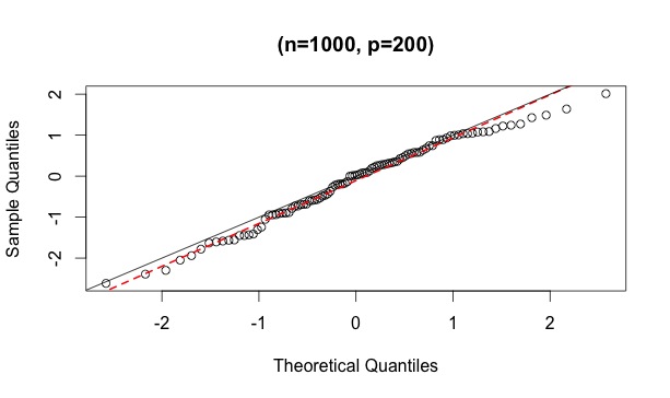
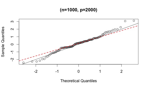
Figure 1: Normal QQ plot for the test statistic for $\widehat{\sigma}$ in (3.25) in Theorem 6 with $n=1000,p=\{200,2000\},g=2,s=8$. The results are produced with 100 replications of the scaled group Lasso. The red dotted line is fitted through $1^{{\rm st}}$ and $3^{{\rm rd}}$ sample quantiles.

In the design setup with $(n=1000,p=200)$, the estimate of $\widehat{\sigma}$ averaged over a 100 replications is 0.997 with a standard deviation of 0.02. In the design setup with $(n=1000,p=2000)$, the estimate of $\widehat{\sigma}$ averaged over a 100 replications is 1.0002 with a standard deviation of 0.02. Additionally Figure 1 shows the Gaussian QQ plots of the test statistic $\sqrt{2n}\left({\widehat{\sigma}}/{\sigma}-1\right)$.

4.2.  Asymptotic distribution of regression parameters

We also seek the empirical validation of the asymptotic convergence of the group $\boldsymbol{\beta}_{G_{j}}$ as described in our theoretical results. For bias correction we take the penalty function in (2.44) to be the Frobenius norm and apply group Lasso based optimization. We also consider a new simulation design which is similar to the earlier design with $(n=1000,p=200)$ and $\sigma=1$. We will consider two different schemes for empirical analysis for asymptotic convergence.

Small group sizes

The true parameter $\boldsymbol{\beta}^{*}$ is simulated to be $(s=40,g=10)$ strong group sparse with its nonzero values in the interval [2,3]. More specifically, $\boldsymbol{\beta}^{*}$ is grouped into groups of sizes $d_{j}=4$ for all $j$. We construct the test statistic of $\boldsymbol{\mu}_{G_{j}}$ as in (2.21) for one of the nonzero groups. The left panel of Figure 2 provides $\chi^{2}_{4}$ based QQ plot for the sample quantiles of our test statistic.

Large group sizes

The true parameter $\boldsymbol{\beta}^{*}$ is simulated to be $(s=40,g=2)$ strong group sparse with its nonzero values between [2,3]. More specifically, $\boldsymbol{\beta}^{*}$ is grouped into 10 groups each of sizes $d_{j}=20$ for all $j$. We let the sparsity of the true parameter $\boldsymbol{\beta}^{*}$ to be $s=40$ contained within 2 separate groups. Again, we construct the test statistic of $\boldsymbol{\mu}_{G_{j}}$ as in (2.21) for one of the nonzero groups. The right panel of Figure 2 shows the QQ plot for this group’s size- normalized test statistic as defined in (2.22). As the figure suggests, for large group sizes asymptotic normality of the group test statistic is empirically supported.

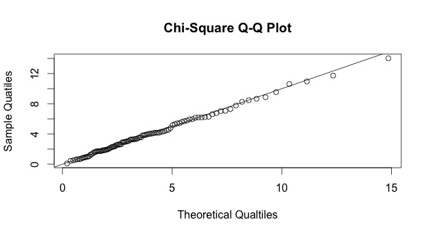
Figure 2: The left panel considers test for a Small group. It shows chi-squared QQ plot for the test statistic $T_{G}$ with $n=1000,p=200,g=10,s=40$. The theoretical quantiles were drawn from $\chi^{2}_{4}$ random variable. The group being tested has size 4. The right panel considers test for a Large group. It shows normal QQ plot for the test statistic $(T^{2}_{G}-|G|)/\sqrt{2|G|}$ with $n=1000,p=200,g=2,s=40$. Here the group size of the test group is 20.

4.3.  Comparison with other methods

In this subsection we compare the performance of our group Lasso methods with other recent methods developed for inference in high dimensional models. In particular we consider three different classes of methods.

Design	Proposed Method					Projection Based					Multi sample-split					Group Bound
	Chi-squared		Normal			Lasso		Ridge			Lasso		Group Lasso
$\boldsymbol{(g,\ s)},\ \boldsymbol{(\rho,\ \tau)}$	FP	TP	FP	TP		FP	TP	FP	TP		FP	TP	FP	TP		FP	TP
(1, 5), (0, 0.1)	0.04	0.11	0.04	0.11		0	0.02	0	0		0	0	0	0		0	0
(1, 5), (0, 0.5)	0	1	0	1		0	1	0.01	0.2		0	0.72	0	0.23		0	0
(1, 5), (0, 1)	0	1	0	1		0	1	0	1		0	1	0	1		0	0
(1, 5), (0.5, 0.1)	0.03	0.3	0.03	0.3		0	0.06	0	0		0	0	0	0		0	0
(1, 5), (0.5, 0.5)	0	1	0	1		0	1	0	0.71		0	0.99	0	0.47		0	0.02
(1, 5), (0.5, 1)	0	1	0	1		0	1	0	1		0	1	0	1		0	0.97
(1, 5), (0.9, 0.1)	0.02	0.45	0.02	0.45		0	0.02	0.2	0.02		0	0.32	0	0		0	0
(1, 5), (0.9, 0.5)	0	1	0	1		0	1	0	0.07		0	0.22	0	0.01		0	0.12
(1, 5), (0.9, 1)	0	1	0	1		0	0.98	0	0.81		0	0.86	0	0.32		0	1
(1, 20), (0.9, 0.1)	0	1	0	1		0	0.38	0	0.01		0	0.05	0	0.00		0	0.04

Table 1: Comparison of true positive and false positive rates for three different choices of block correlation $\rho$ and three choices of signal parameter $\tau$. The scale parameter $\sigma=1$ in all cases. The results are based on 100 replications for testing the nonzero group (for TP) and first zero group (FP). Performance of all the tests are good for the strong signal ($\tau$= 1). For the weak signal $\tau=0.1$, group Lasso clearly out-performs other methods.

Projection based:

For the projection based methods, we consider two cases. 1) The Ridge estimation based testing with correction for projection bias that was developed in Bühlmann (2013). 2) The Lasso relaxed projection followed by bias correction idea developed in Zhang and Zhang (2014) which is similar to the de-sparsified Lasso in van de Geer et al. (2014). These methods are adapted for testing of groups of variables adjustment of individual $p$-values; see Dezeure et al. (2014).

Sample split based:

The idea of single sample splitting was developed in Wasserman and Roeder (2009) which involves splitting the sample into two parts. The first part is used to select variables and the second to construct $p$-values for the selected variables in the first model. The final step is to adjust the $p$-values for control of the familywise error rate (FWER). Due to the variability of the $p$-values for different splittings, Meinshausen, Meier and Bühlmann (2009) proposed multi sample-splitting idea which involves running the single sample splitting $B$ times and aggregating the $B$ adjusted $p$-values. We employ the multi sample-splitting with two different variable selection procedures: Lasso and group Lasso. For Lasso, the groupwise $p$-value is obtained by Bonferroni adjustments.

Group bound:

The final procedure we consider is the group bound method developed in Meinshausen (2014). One advantage of this method is that it doesn’t require any assumptions on the design matrix.

Implementation of all the above methods are available in the R package hdi; see also Dezeure et al. (2014).

Simulation Design: We consider a very simple simulation design where the design matrix ${\rm\textbf{X}}\in{\mathbb{R}}^{n\times p}$ is assumed to have iid rows with each row following $\mathsf{N}(\boldsymbol{0},\boldsymbol{\Sigma})$, where $\boldsymbol{\Sigma}$ is assumed to be a correlation matrix having a block diagonal structure with block size $k=5$. We take $n=100$ and $p=200$ so that $\boldsymbol{\Sigma}$ has $M=$40 blocks. Within each block, the correlation is assumed to be $\rho$. For our simulations, we consider three possible choices of $\rho$ namely $\{0,0.5,0.9\}$.

The true parameter $\boldsymbol{\beta}$ is assumed to have the group structure as defined by the block structure of X. Moreover we assume only the first group has nonzero signals with all of them having the same value $\tau>0$. Thus $\boldsymbol{\beta}^{*}$ is of the form,

$$\boldsymbol{\beta}^{*}=(\underbrace{\tau,\tau,\tau,\tau,\tau}_{\text{group 1}},\underbrace{0,0,0,0,0}_{\text{group 2}},\cdots,\underbrace{0,0,0,0,0}_{\text{group 40}})$$

Thus in all these cases, the true signal $\boldsymbol{\beta}^{*}$ is $(g=1,s=5)$ strong group sparse. We consider three choices of the signal parameter $\tau$: $\{0.1,0.5,1\}$.

We also consider an additional scenario, where we take $k=20$ so that number of groups $M=10$ (The last line of Table 1). For this case we only compare the performance for signal strength $\tau=0.1$ which highlights the performance of group Lasso.

The responses are simulated by $\boldsymbol{y}={\rm\textbf{X}}\boldsymbol{\beta}^{*}+\boldsymbol{\varepsilon}$ where $\boldsymbol{\varepsilon}\sim\mathsf{N}(0,\sigma)$. We take the true scale parameter $\sigma=1$ in all simulation designs and estimate $\sigma$ via scaled group Lasso. For application of the group Lasso based testing, we take the group weights equal to $\omega_{j}=5(\sqrt{d_{j}/n}+\sqrt{(2/n)\log(M)})$ where $M=40$ and $d_{j}=5$ for group sizes=5 and $d_{j}=20$ for group sizes=20.

In Table 1, we provide a comparison of the true positive (TP) and false positive (FP) rates for 100 replications. It is clear from the table that group Lasso performs comparably or better than all the other methods. The false positive rates of all the methods are either 0 or close to zero for most of the designs. The true positive (TP) rate (power) of group Lasso method clearly dominates those of the other methods especially when the signal is not strong: $\tau=0.1$. One rationale for this would be the accumulation of small signals in the $\ell_{2}$ norm for the group that is used for the group Lasso. For group bound method, clearly the performance becomes comparable to group Lasso as the blockwise correlation $\rho$ is increased. This phenomenon is also observed for group Lasso procedure to a certain extent.

5.  Summary and Discussion

We have considered statistical inference of variable groups in a high-dimensional linear regression setup. In particular we show the benefit of grouping in constructing chi-squared-type procedures for group inference. We construct such procedures via bias correction and group Lasso based relaxed projection. We show the validity of such approximate chi-squared-type inference under sample size conditions that could be potentially much weaker than the requirements for Lasso based procedures. This particular scaling also offers us valid statistical inference for a group of possibly unbounded number of variables.

A key step of our methodology concerns the nonconvex optimization scheme (2.34) over the set of orthogonal projection matrices. To the best of our knowledge, solution of an optimization problem as in (2.34) is not yet well studied, either algorithmically or analytically. However, we have proposed a convexation of (2.34) via a multivariate group Lasso with a weighted nuclear or Frobenius norm penalty, which provides feasible solutions for the optimization problem. As discussed in Remark 1, our theoretical results only requires feasibility solutions of the optimization scheme. As the multivariate group Lasso with Frobenius norm penalty can be carried out using the group Lasso program, an interesting direction of research would be to develop efficient algorithm for the group nuclear norm penalty.

Since our results can be directly applied to statistical inference for groups of variables with possibly unbounded sizes, application of our procedures for sparse nonparametric additive models (Ravikumar et al., 2009) would be another future direction of research.

Appendix A Appendix

This appendix provides proof of

Proof of Proposition 1. (i) Since both ${\rm\textbf{Z}}_{G}$ and ${\rm\textbf{X}}_{G}$ are $n\times|G|$ matrices,

$$|G|=\hbox{rank}({\rm\textbf{Z}}_{G}^{T}{\rm\textbf{X}}_{G})\leq\hbox{rank}({\rm\textbf{X}}_{G})\wedge\hbox{rank}({\rm\textbf{Z}}_{G})\leq|G|\wedge n,$$

so that $\hbox{rank}({\rm\textbf{P}}_{G})=\hbox{rank}({\rm\textbf{P}}_{G}{\rm\textbf{X}}_{G})=|G|$ and ${\rm\textbf{P}}_{G}={\rm\textbf{P}}_{G,0}$. It follows that ${\rm\textbf{P}}_{G}{\rm\textbf{X}}_{G}({\rm\textbf{P}}_{G}{\rm\textbf{X}}_{G})^{\dagger}{\rm\textbf{P}}_{G}={\rm\textbf{P}}_{G}$. As ${\rm\textbf{Z}}_{G}^{T}{\rm\textbf{X}}_{G}$ is a $|G|\times|G|$ invertible matrix, ${\rm\textbf{P}}_{G}{\rm\textbf{X}}_{G}({\rm\textbf{Z}}_{G}^{T}{\rm\textbf{X}}_{G})^{-1}{\rm\textbf{Z}}_{G}^{T}={\rm\textbf{P}}_{G}$. Since $\hbox{rank}({\rm\textbf{P}}_{G}{\rm\textbf{X}}_{G})=|G|$, we are allowed to cancel ${\rm\textbf{P}}_{G}{\rm\textbf{X}}_{G}$ to obtain $({\rm\textbf{P}}_{G}{\rm\textbf{X}}_{G})^{\dagger}{\rm\textbf{P}}_{G}=({\rm\textbf{Z}}_{G}^{T}{\rm\textbf{X}}_{G})^{\dagger}{\rm\textbf{Z}}_{G}^{T}$. This proves the first equality in (2.15). The second equality in (2.15) then follows from

$$({\rm\textbf{P}}_{G}{\rm\textbf{X}}_{G})^{\dagger}{\rm\textbf{P}}_{G}\big{(}{\rm\textbf{X}}_{G}\boldsymbol{\beta}_{G}^{*}-{\rm\textbf{X}}_{G}{\widehat{\boldsymbol{\beta}}}_{G}^{(init)}\big{)}=\boldsymbol{\beta}_{G}^{*}-{\widehat{\boldsymbol{\beta}}}_{G}^{(init)},$$

(2.2) and its estimated version, and the definition of the remainder term.

(ii) Let ${\rm\textbf{Z}}_{1}={\rm\textbf{P}}_{G}{\rm\textbf{Z}}_{G}$. As ${\rm\textbf{P}}_{G}={\rm\textbf{P}}_{G}{\rm\textbf{P}}_{G,0}$ is the orthogonal projection to ${\cal R}({\rm\textbf{Z}}_{1})$, ${\rm\textbf{Z}}_{G}^{T}{\rm\textbf{X}}_{G}={\rm\textbf{Z}}_{G}^{T}{\rm\textbf{P}}_{G,0}{\rm\textbf{Q}}_{G}{\rm\textbf{X}}_{G}={\rm\textbf{Z}}_{1}^{T}{\rm\textbf{P}}_{G}{\rm\textbf{Q}}_{G}{\rm\textbf{X}}_{G}$ and $\hbox{rank}({\rm\textbf{X}}_{G})=\hbox{rank}({\rm\textbf{P}}_{G}{\rm\textbf{Q}}_{G})=\hbox{rank}({\rm\textbf{Z}}_{1}^{T}{\rm\textbf{X}}_{G})$, so that

$$({\rm\textbf{Z}}_{G}^{T}{\rm\textbf{X}}_{G})^{\dagger}=({\rm\textbf{Z}}_{1}^{T}{\rm\textbf{P}}_{G}{\rm\textbf{Q}}_{G}{\rm\textbf{X}}_{G})^{\dagger}={\rm\textbf{X}}_{G}^{\dagger}({\rm\textbf{P}}_{G}{\rm\textbf{Q}}_{G})^{\dagger}({\rm\textbf{Z}}_{1}^{T})^{\dagger}.$$

Consequently, as ${\rm\textbf{Q}}_{G}({\rm\textbf{P}}_{G}{\rm\textbf{Q}}_{G})^{\dagger}=({\rm\textbf{P}}_{G}{\rm\textbf{Q}}_{G})^{\dagger}=({\rm\textbf{P}}_{G}{\rm\textbf{Q}}_{G})^{\dagger}{\rm\textbf{P}}_{G}$ and $({\rm\textbf{Z}}_{1}^{T})^{\dagger}{\rm\textbf{Z}}_{G}^{T}={\rm\textbf{P}}_{G}$, we have

$${\widehat{\boldsymbol{\mu}}}_{G}-{\widehat{\boldsymbol{\mu}}}_{G}^{(init)} = {\rm\textbf{X}}_{G}({\rm\textbf{Z}}_{G}^{T}{\rm\textbf{X}}_{G})^{\dagger}{\rm\textbf{Z}}_{G}^{T}\Big{(}\boldsymbol{y}-{\rm\textbf{X}}{\widehat{\boldsymbol{\beta}}}^{(init)}\Big{)}$$

$$= {\rm\textbf{X}}_{G}{\rm\textbf{X}}_{G}^{\dagger}({\rm\textbf{P}}_{G}{\rm\textbf{Q}}_{G})^{\dagger}({\rm\textbf{Z}}_{1}^{T})^{\dagger}{\rm\textbf{Z}}_{G}^{T}\Big{(}\boldsymbol{y}-{\rm\textbf{X}}{\widehat{\boldsymbol{\beta}}}^{(init)}\Big{)}$$

$$= ({\rm\textbf{P}}_{G}{\rm\textbf{Q}}_{G})^{\dagger}{\rm\textbf{P}}_{G}\Big{(}\boldsymbol{y}-{\rm\textbf{X}}{\widehat{\boldsymbol{\beta}}}^{(init)}\Big{)}.$$

This gives (2.16). As ${\rm\textbf{Q}}_{G}({\rm\textbf{Z}}_{G}^{T}{\rm\textbf{Q}}_{G})^{\dagger}{\rm\textbf{Z}}_{G}^{T}=({\rm\textbf{P}}_{G}{\rm\textbf{Q}}_{G})^{\dagger}{\rm\textbf{P}}_{G}^{T}$ by the same proof, (2.13) also holds. Finally, (2.18) follows from (2.14) and (2.2).

Proof of Lemma 1. Let $\boldsymbol{u}_{j},1\leq j\leq r_{k}$, be the eigenvectors of ${\rm\textbf{B}}_{k}^{T}\boldsymbol{\Sigma}{\rm\textbf{B}}_{k}$ corresponding to positive eigenvalues and ${\rm\textbf{U}}_{k}=(\boldsymbol{u}_{1},\ldots,\boldsymbol{u}_{r_{k}})$. Let ${\rm\textbf{Z}}_{k}={\rm\textbf{X}}{\rm\textbf{B}}_{k}(({\rm\textbf{B}}_{k}^{T}\boldsymbol{\Sigma}{\rm\textbf{B}}_{k})^{\dagger})^{1/2}{\rm\textbf{U}}_{k}\in\mathbb{R}^{n\times r_{k}}$. We have $\mathbb{E}{\rm\textbf{Z}}_{k}={\bf 0}$, $\mathbb{E}({\rm\textbf{Z}}_{k}^{T}{\rm\textbf{Z}}_{k}/n)={\rm\textbf{I}}_{r_{k}\times r_{k}}$, $\mathbb{E}({\rm\textbf{Z}}_{1}^{T}{\rm\textbf{Z}}_{2}/n)={\rm\textbf{U}}_{1}^{T}\boldsymbol{\Omega}_{1,2}{\rm\textbf{U}}_{2}$, and

$$\sup_{\|\boldsymbol{b}\|_{2}\leq 1}\ \mathbb{E}\exp\left(\frac{(\boldsymbol{e}_{i}^{T}{\rm\textbf{Z}}_{k}\boldsymbol{b})^{2}}{v_{0}}+\frac{1}{v_{0}}\right)\leq 2,\ k=1,2.$$

Moreover, ${\rm\textbf{P}}_{k}={\rm\textbf{Z}}_{k}({\rm\textbf{Z}}_{k}^{T}{\rm\textbf{Z}}_{k})^{{\dagger}}{\rm\textbf{Z}}_{k}^{T}$ and $\|{\rm\textbf{U}}_{1}^{T}\boldsymbol{\Omega}_{1,2}{\rm\textbf{U}}_{2}\|_{S}=\|\boldsymbol{\Omega}_{1,2}\|_{S}\leq 1$.

For $1\leq j\leq k\leq 2$ and any vectors $\boldsymbol{v}_{k}\in\mathbb{R}^{r_{k}}$ with $\|\boldsymbol{v}_{k}\|_{2}=1$,

$$\boldsymbol{v}_{j}^{T}\Big{(}{\rm\textbf{Z}}_{j}^{T}{\rm\textbf{Z}}_{k}/n-\mathbb{E}{\rm\textbf{Z}}_{j}^{T}{\rm\textbf{Z}}_{k}/n\Big{)}\boldsymbol{v}_{k}=\frac{1}{n}\sum_{i=1}^{n}\Big{\{}(\boldsymbol{e}_{i}^{T}{\rm\textbf{Z}}_{j}\boldsymbol{v}_{j})(\boldsymbol{e}_{i}^{T}{\rm\textbf{Z}}_{k}\boldsymbol{v}_{k})-\boldsymbol{v}_{j}^{T}\mathbb{E}({\rm\textbf{Z}}_{j}^{T}{\rm\textbf{Z}}_{k}/n)\boldsymbol{v}_{k}\Big{\}}$$

is an average of iid variables with

$$\mathbb{E}\exp\left(\frac{(\boldsymbol{e}_{i}^{T}{\rm\textbf{Z}}_{j}\boldsymbol{v}_{j})(\boldsymbol{e}_{i}^{T}{\rm\textbf{Z}}_{k}\boldsymbol{v}_{k})-\boldsymbol{v}_{j}^{T}\mathbb{E}({\rm\textbf{Z}}_{j}^{T}{\rm\textbf{Z}}_{k}/n)\boldsymbol{v}_{k}}{v_{0}}\right)$$

$$\leq \left\{\prod_{k=1}^{2}\sqrt{\mathbb{E}\exp\left((\boldsymbol{e}_{i}^{T}{\rm\textbf{Z}}_{k}\boldsymbol{v}_{k})^{2}/v_{0}\right)}\right\}e^{1/v_{0}}$$

$$\leq 2.$$

Since the size of an $\epsilon$-net of the unit ball in ${\mathbb{R}}^{r_{k}}$ is bounded by $(1+2/\epsilon)^{r_{k}}$, the Bernstein inequality implies that for $r^{*}=r_{1}+r_{2}$ and a certain numerical constant $C_{0}$,

$$\mathbb{P}\Big{\{}\|{\rm\textbf{Z}}_{j}^{T}{\rm\textbf{Z}}_{k}/n-\mathbb{E}({\rm\textbf{Z}}_{j}^{T}{\rm\textbf{Z}}_{k}/n)\|_{S}>C_{0}v_{0}\max\Big{(}\sqrt{t/n+r^{*}/n},t/n+r^{*}/n\Big{)}\Big{\}}\leq e^{-t}/3.$$

This yields (2.41) as $\|{\rm\textbf{U}}_{1}^{T}\boldsymbol{\Delta}{\rm\textbf{U}}_{2}\|_{S}=\|\boldsymbol{\Delta}\|_{S}$ for all $\boldsymbol{\Delta}$ of proper dimension.

Suppose $\hbox{rank}({\rm\textbf{P}}_{k})=r_{k}$. Let $r_{0}=\hbox{rank}({\rm\textbf{P}}_{1}{\rm\textbf{P}}_{2})$ and $1\geq\widehat{\lambda}_{1}\geq\cdots\geq\widehat{\lambda}_{r_{0}}>0$ be the (nonzero) singular values of ${\rm\textbf{P}}_{1}{\rm\textbf{P}}_{2}$. We have $\|{\rm\textbf{P}}_{1}{\rm\textbf{P}}_{2}\|_{S}=\widehat{\lambda}_{1}$ and $\|{\rm\textbf{P}}_{1}{\rm\textbf{P}}_{2}^{\perp}\|_{S}=\|{\rm\textbf{P}}_{1}-{\rm\textbf{P}}_{2}\|_{S}=\sqrt{1-\widehat{\lambda}_{\min}^{2}}$ with $\widehat{\lambda}_{\min}=\widehat{\lambda}_{r_{0}}I\{r_{0}=r_{1}=r_{2}\}$. By definition,

$${\rm\textbf{P}}_{1}{\rm\textbf{P}}_{2}={\rm\textbf{Z}}_{1}({\rm\textbf{Z}}_{1}^{T}{\rm\textbf{Z}}_{1})^{-1}{\rm\textbf{Z}}_{1}^{T}{\rm\textbf{Z}}_{2}({\rm\textbf{Z}}_{2}^{T}{\rm\textbf{Z}}_{2})^{-1}{\rm\textbf{Z}}_{2}^{T}.$$

Since $({\rm\textbf{Z}}_{k}^{T}{\rm\textbf{Z}}_{k})^{-1/2}{\rm\textbf{Z}}_{k}^{T}$ are unitary maps from the range of ${\rm\textbf{P}}_{k}$ to $\mathbb{R}^{r_{k}}$, the singular values of ${\rm\textbf{P}}_{1}{\rm\textbf{P}}_{2}$ is the same as those of

$$({\rm\textbf{Z}}_{1}^{T}{\rm\textbf{Z}}_{1})^{-1/2}{\rm\textbf{Z}}_{1}^{T}{\rm\textbf{Z}}_{2}({\rm\textbf{Z}}_{2}^{T}{\rm\textbf{Z}}_{2})^{-1/2}.$$

Now suppose that $\|{\rm\textbf{Z}}_{j}^{T}{\rm\textbf{Z}}_{k}/n-\mathbb{E}({\rm\textbf{Z}}_{j}^{T}{\rm\textbf{Z}}_{k}/n)\|_{S}\leq C_{0}v_{0}\sqrt{t/n+r/n}\leq\epsilon_{0}<1$ for $1\leq j\leq k\leq 2$. Recall that $1\geq\lambda_{1}\geq\cdots\geq\lambda_{r}>0$ are the nonzero singular values of $\boldsymbol{\Omega}_{1,2}$ and $\lambda_{\min}=\lambda_{r}I\{r=r_{1}=r_{2}\}$. As $\mathbb{E}({\rm\textbf{Z}}_{k}^{T}{\rm\textbf{Z}}_{k}/n)={\rm\textbf{I}}_{r_{k}\times r_{k}}$, we have $\hbox{rank}({\rm\textbf{P}}_{k})=r_{k}$. Moreover, as $\mathbb{E}({\rm\textbf{Z}}_{1}^{T}{\rm\textbf{Z}}_{2}/n)={\rm\textbf{U}}_{1}^{T}\boldsymbol{\Omega}_{1,2}{\rm\textbf{U}}_{2}$ with unitary maps ${\rm\textbf{U}}_{1}$ and ${\rm\textbf{U}}_{2}$, the Weyl inequality implies that

$$\widehat{\lambda}_{1}\leq\frac{\lambda_{1}(1+\epsilon_{0})}{1-\epsilon_{0}},\quad\widehat{\lambda}_{\min}\geq\frac{\lambda_{\min}(1-\epsilon_{0})}{1+\epsilon_{0}}.$$

Thus, (2.42) holds. As the conditions for $\lambda_{1}<1$ and $\lambda_{\min}>0$ follow from the positive-definiteness of $\boldsymbol{\Sigma}$, the proof is complete.

Proof of Theorem 5. The KKT conditions for the group Lasso asserts that

$$\begin{array}[]{lc}\dfrac{1}{n}{\rm\textbf{X}}_{G_{j}}^{T}(\boldsymbol{y}-{\rm\textbf{X}}{\widehat{\boldsymbol{\beta}}})=\omega_{j}{\widehat{\boldsymbol{\beta}}}_{G_{j}}/\|{\widehat{\boldsymbol{\beta}}}_{G_{j}}\|_{2},&{\widehat{\boldsymbol{\beta}}}_{G_{j}}\neq\boldsymbol{0},\\[8.5359pt] \dfrac{1}{n}\|{\rm\textbf{X}}_{G_{j}}^{T}(\boldsymbol{y}-{\rm\textbf{X}}{\widehat{\boldsymbol{\beta}}})\|_{2}\leq\omega_{j},&{\widehat{\boldsymbol{\beta}}}_{G_{j}}=\boldsymbol{0}.\end{array}$$ (A.3)

Let $\boldsymbol{h}={\widehat{\boldsymbol{\beta}}}-\boldsymbol{\beta}^{*}$. It follows that in the event ${\cal E}$

$$\frac{\|{\rm\textbf{X}}_{G_{j}}^{T}{\rm\textbf{X}}\boldsymbol{h}\|_{2}}{\omega_{j}n}=\frac{\|{\rm\textbf{X}}_{G_{j}}^{T}({\rm\textbf{X}}{\widehat{\boldsymbol{\beta}}}-\boldsymbol{y}+\boldsymbol{\varepsilon})\|_{2}}{\omega_{j}n}\leq 1+\frac{\|{\rm\textbf{X}}_{G_{j}}^{T}\boldsymbol{\varepsilon}\|_{2}}{\omega_{j}n}\leq\frac{2\xi}{\xi+1}.$$ (A.4)

It also follows from (A.3) that in the event ${\cal E}$

$$\boldsymbol{h}_{G_{j}}^{T}{\rm\textbf{X}}^{T}_{G_{j}}{\rm\textbf{X}}\boldsymbol{h}/n$$ (A.5)

$$= \boldsymbol{h}_{G_{j}}^{T}{\rm\textbf{X}}^{T}_{G_{j}}({\rm\textbf{X}}{\widehat{\boldsymbol{\beta}}}-\boldsymbol{y}+\boldsymbol{\varepsilon})/n$$ (A.6)

$$\leq \begin{cases}\omega_{j}\|\boldsymbol{h}_{G_{j}}\|_{2}+|\boldsymbol{h}_{G_{j}}^{T}{\rm\textbf{X}}^{T}_{G_{j}}\boldsymbol{\varepsilon}|/n,&j\in S^{*},\cr-\omega_{j}\|\boldsymbol{h}_{G_{j}}\|_{2}+|\boldsymbol{h}_{G_{j}}^{T}{\rm\textbf{X}}^{T}_{G_{j}}\boldsymbol{\varepsilon}|/n,&j\not\in S^{*},\end{cases}$$ (A.7)

$$\leq \begin{cases}\omega_{j}\|\boldsymbol{h}_{G_{j}}\|_{2}2\xi/(\xi+1),\ j\in S^{*},\cr-\omega_{j}\|\boldsymbol{h}_{G_{j}}\|_{2}2/(\xi+1),\ j\not\in S^{*}.\end{cases}$$ (A.8)

Summing the above inequality over $j$, we have

$$\|{\rm\textbf{X}}\boldsymbol{h}\|_{2}^{2}/n\leq\frac{2\xi}{\xi+1}\sum_{j\in S^{*}}\omega_{j}\|\boldsymbol{u}_{G_{j}}\|_{2}-\frac{2}{\xi+1}\sum_{j\not\in S^{*}}\omega_{j}\|\boldsymbol{u}_{G_{j}}\|_{2}.$$

This and (A.5) implies $\boldsymbol{h}\in{\mathscr{C}}^{(G)}_{-}(\xi,\boldsymbol{\omega},S^{*})$. Thus, by (3.6) and (A.4)

$$\|{\rm\textbf{X}}\boldsymbol{h}\|_{2}^{2}/n \leq \{2\xi/(\xi+1)\}\sum_{j\in S^{*}}\omega_{j}\|{\widehat{\boldsymbol{\beta}}}_{G_{j}}-\boldsymbol{\beta}_{G_{j}}^{*}\|_{2}$$

$$\leq \{2\xi/(\xi+1)\}\max_{j}\omega^{-1}_{j}\|{\rm\textbf{X}}_{G_{j}}^{T}{\rm\textbf{X}}\boldsymbol{h}\|_{2}\hbox{$\sum_{j\in S^{*}}$}\omega_{j}^{2}/\{n\,{\rm SCIF}^{(G)}_{1}(\xi,\boldsymbol{\omega},S^{*},S^{*})\}$$

$$\leq \{2\xi/(\xi+1)\}^{2}\hbox{$\sum_{j\in S^{*}}$}\omega_{j}^{2}/\{n\,{\rm SCIF}^{(G)}_{1}(\xi,\boldsymbol{\omega},S^{*},S^{*})\}.$$

Similarly, (3.6) and (A.4) yield

$$\Big{(}\hbox{$\sum_{j=1}^{M}$}\omega_{j}^{2}(\|\boldsymbol{h}_{G_{j}}\|_{2}/\omega_{j})^{q}\Big{)}^{1/q} \leq \big{(}\hbox{$\sum_{j\in S^{*}}$}\omega_{j}^{2}\big{)}^{1/q}\max_{j}\omega^{-1}_{j}\|{\rm\textbf{X}}_{G_{j}}^{T}{\rm\textbf{X}}\boldsymbol{h}\|_{2}/\{{\rm SCIF}^{(G)}_{q}(\xi,\boldsymbol{\omega},S^{*})\}$$

$$\leq \{2\xi/(\xi+1)\}\big{(}\hbox{$\sum_{j\in S^{*}}$}\omega_{j}^{2}\big{)}^{1/q}\{{\rm SCIF}^{(G)}_{q}(\xi,\boldsymbol{\omega},S^{*},T^{*})\}.$$

Finally, we prove (3.12). Let ${\rm\textbf{Q}}_{G_{j}}$ be the orthogonal projection to the range of ${\rm\textbf{X}}_{G_{j}}$. As $\boldsymbol{\varepsilon}\sim\mathsf{N}_{n}(\boldsymbol{0},\sigma^{2}{\rm\textbf{I}}_{n})$, $\|{\rm\textbf{Q}}_{G_{j}}\boldsymbol{\varepsilon}/\sigma\|_{2}^{2}\sim\chi^{2}_{d_{j}^{\prime}}$ with $d_{j}^{\prime}=\hbox{rank}({\rm\textbf{Q}}_{G_{j}})\leq d_{j}$. Thus, it follows from the Gaussian concentration inequality that for any $0<\delta<1$, with probability at least $1-\delta$,

$$\|{\rm\textbf{X}}_{G_{j}}^{T}\boldsymbol{\varepsilon}\|_{2}/(\sigma\|{\rm\textbf{X}}_{G_{j}}\|_{S})\leq\|{\rm\textbf{Q}}_{G_{j}}\boldsymbol{\varepsilon}/\sigma\|_{2}\leq\sqrt{n}\left\{\sqrt{d_{j}}+\sqrt{2\log(1/\delta)}\right\}.$$

The result in (3.12) follows by an application of the union bound.

Proof of Lemma 2. For $\eta\geq 0$ define

$${\cal L}_{\boldsymbol{\omega}}(\boldsymbol{\beta},\sigma,\eta)=\frac{\|\boldsymbol{y}-{\rm\textbf{X}}\boldsymbol{\beta}\|_{2}^{2}}{2n\sigma}+\frac{\sigma}{2}+\sum_{j=1}^{M}\omega_{j}\|\boldsymbol{\beta}_{G_{j}}\|_{2}^{1+\eta}+\frac{\eta\sigma^{2}}{2}$$

and ${\widehat{\boldsymbol{\beta}}}(\sigma\boldsymbol{\omega},\eta)=\mathop{\rm arg\,min}_{\boldsymbol{\beta}}\ {\cal L}_{\boldsymbol{\omega}}(\boldsymbol{\beta},\sigma,\eta)$. As ${\cal L}_{\boldsymbol{\omega}}(\boldsymbol{\beta},\sigma,\eta)$ is convex in $(\boldsymbol{\beta},\sigma)$, the profile loss ${\cal L}_{\boldsymbol{\omega}}({\widehat{\boldsymbol{\beta}}}(\sigma\boldsymbol{\omega},\eta),\sigma,\eta)$ is convex in $\sigma$ for all $\eta\geq 0$. Note that for $\eta>0$

$$\dfrac{\partial}{\partial\sigma}{\cal L}_{\boldsymbol{\omega}}({\widehat{\boldsymbol{\beta}}}(\sigma\boldsymbol{\omega},\eta),\sigma,\eta)$$

$$= \left\{\dfrac{\partial}{\partial\boldsymbol{\theta}}{\cal L}_{\boldsymbol{\omega}}(\boldsymbol{\theta},\sigma,\eta)\Big{|}_{\boldsymbol{\theta}={\widehat{\boldsymbol{\beta}}}(\sigma\boldsymbol{\omega},\eta)}\right\}^{T}\dfrac{\partial{\widehat{\boldsymbol{\beta}}}(\sigma\boldsymbol{\omega},\eta)}{\partial\sigma}+\dfrac{\partial}{\partial t}{\cal L}_{\boldsymbol{\omega}}({\widehat{\boldsymbol{\beta}}}(\sigma\boldsymbol{\omega}),t,\eta)\Big{|}_{t=\sigma}$$

$$= 1/2-\|\boldsymbol{y}-{\rm\textbf{X}}{\widehat{\boldsymbol{\beta}}}(\sigma\boldsymbol{\omega},\eta)\|_{2}^{2}/(2n\sigma^{2})+\eta\sigma$$

as all derivatives involved are continuous. Moreover, as ${\cal L}_{\boldsymbol{\omega}}(\boldsymbol{\beta},\sigma)={\cal L}_{\boldsymbol{\omega}}(\boldsymbol{\beta},\sigma,0)$ is strictly convex in ${\rm\textbf{X}}\boldsymbol{\beta}$,

$$\lim_{\eta\to 0+}\dfrac{\partial}{\partial\sigma}{\cal L}_{\boldsymbol{\omega}}({\widehat{\boldsymbol{\beta}}}(\sigma\boldsymbol{\omega},\eta),\sigma,\eta)\to 1/2-\|\boldsymbol{y}-{\rm\textbf{X}}{\widehat{\boldsymbol{\beta}}}(\sigma\boldsymbol{\omega})\|_{2}^{2}/(2n\sigma^{2}).$$

Consequently,

$${\cal L}_{\boldsymbol{\omega}}({\widehat{\boldsymbol{\beta}}}(\sigma_{2}\boldsymbol{\omega}),\sigma_{2})-{\cal L}_{\boldsymbol{\omega}}({\widehat{\boldsymbol{\beta}}}(\sigma_{1}\boldsymbol{\omega}),\sigma_{1}) = \lim_{\eta\to 0+}\int_{\sigma_{1}}^{\sigma_{2}}\Big{\{}\dfrac{\partial}{\partial\sigma}{\cal L}_{\boldsymbol{\omega}}({\widehat{\boldsymbol{\beta}}}(\sigma\boldsymbol{\omega},\eta),\sigma,\eta)\Big{\}}d\sigma$$

$$= \int_{\sigma_{1}}^{\sigma_{2}}\Big{\{}1/2-\|\boldsymbol{y}-{\rm\textbf{X}}{\widehat{\boldsymbol{\beta}}}(\sigma\boldsymbol{\omega})\|_{2}^{2}/(2n\sigma^{2})\Big{\}}d\sigma.$$

All other claims follow from the joint convexity of ${\cal L}_{\boldsymbol{\omega}}(\boldsymbol{\beta},\sigma)$ and the strict convexity of the loss function in ${\rm\textbf{X}}\boldsymbol{\beta}$.

Proof of Theorem 6. We follow the proof in Sun and Zhang (2012b). Let $t\geq\sigma^{*}/\sqrt{1+\tau_{-}}$ and $\boldsymbol{h}_{G_{j}}={\widehat{\boldsymbol{\beta}}}_{G_{j}}(t\boldsymbol{\omega})-\boldsymbol{\beta}^{*}_{G_{j}}$. As the oracle noise level is $({\sigma^{*}})^{2}=\|\boldsymbol{y}-{\rm\textbf{X}}\boldsymbol{\beta}^{*}\|_{2}^{2}/n$, we have

$$({\sigma^{*}})^{2}-\|\boldsymbol{y}-{\rm\textbf{X}}{\widehat{\boldsymbol{\beta}}}(t\boldsymbol{\omega})\|_{2}^{2}/n=({\rm\textbf{X}}\boldsymbol{h})^{T}(2\boldsymbol{\varepsilon}-{\rm\textbf{X}}\boldsymbol{h})/n=({\rm\textbf{X}}\boldsymbol{h})^{T}(\boldsymbol{\varepsilon}+\boldsymbol{y}-{\rm\textbf{X}}{\widehat{\boldsymbol{\beta}}}(t\boldsymbol{\omega}))/n.$$ (A.9)

Suppose ${\cal E}$ happens so that $\|{\rm\textbf{X}}_{G_{j}}^{T}\boldsymbol{\varepsilon}\|_{2}/n\leq t\omega_{j}(\xi-1)/(\xi+1)$. It follows that

$$\left|({\rm\textbf{X}}\boldsymbol{h})^{T}\boldsymbol{\varepsilon}/n\right|=\left|\sum^{M}_{j=1}\boldsymbol{h}^{T}_{G_{j}}{\rm\textbf{X}}_{G_{j}}^{T}\boldsymbol{\varepsilon}/n\right|\leq\frac{\xi-1}{\xi+1}\sum^{M}_{j=1}t\omega_{j}\|\boldsymbol{h}_{G_{j}}\|_{2}.$$

Moreover, the KKT condition implies

$$\left|\boldsymbol{h}^{T}{\rm\textbf{X}}^{T}(\boldsymbol{y}-{\rm\textbf{X}}{\widehat{\boldsymbol{\beta}}}(t\boldsymbol{\omega}))/n\right|=\left|\sum^{M}_{j=1}\boldsymbol{h}_{G_{j}}^{T}{\rm\textbf{X}}_{G_{j}}^{T}(\boldsymbol{y}-{\rm\textbf{X}}{\widehat{\boldsymbol{\beta}}}(t\boldsymbol{\omega}))/n\right|\leq\sum^{M}_{j=1}t\omega_{j}\|\boldsymbol{h}_{G_{j}}\|_{2}.$$

As $({\rm\textbf{X}}\boldsymbol{h})^{T}(2\boldsymbol{\varepsilon}-{\rm\textbf{X}}\boldsymbol{h})/n\leq 2({\rm\textbf{X}}\boldsymbol{h})^{T}\boldsymbol{\varepsilon}/n$, inserting these inequalities to (A.9) yields

$$-\left(\frac{\xi-1}{\xi+1}+1\right)\sum^{M}_{j=1}t\omega_{j}\|\boldsymbol{h}_{G_{j}}\|_{2}\leq{{\sigma^{*}}}^{2}-\|\boldsymbol{y}-{\rm\textbf{X}}{\widehat{\boldsymbol{\beta}}}(t\boldsymbol{\omega})\|_{2}^{2}/n\leq 2\frac{\xi-1}{\xi+1}\sum^{M}_{j=1}t\omega_{j}\|\boldsymbol{h}_{G_{j}}\|_{2}.$$

A rescaled version ${\widehat{\boldsymbol{\beta}}}(t\boldsymbol{\omega})$ can be written as

$$\frac{{\widehat{\boldsymbol{\beta}}}(t\boldsymbol{\omega})}{t}=\mathop{\rm arg\,min}_{\boldsymbol{b}}\left\{\dfrac{\|\boldsymbol{y}/t-{\rm\textbf{X}}\boldsymbol{b}\|_{2}^{2}}{2n}+\sum^{M}_{j=1}\omega_{j}\|\boldsymbol{b}_{G_{j}}\|_{2}\right\}$$

as the group Lasso estimator with target $\boldsymbol{\beta}^{*}/t$ and noise vector $\boldsymbol{\varepsilon}/t$. As $t\geq\sigma^{*}/\sqrt{1+\tau_{-}}$, the condition of Theorem 5 is satisfied with the rescaled noise $\boldsymbol{\varepsilon}/t$, so that

$$t^{-1}\sum^{M}_{j=1}\omega_{j}\|\boldsymbol{h}_{G_{j}}\|_{2}=\sum^{M}_{j=1}\omega_{j}\|{\widehat{\boldsymbol{\beta}}}_{G_{j}}(t\boldsymbol{\omega})/t-\boldsymbol{\beta}^{*}_{G_{j}}/t\|_{2}<\mu(\boldsymbol{\omega},\xi).$$

As $\tau_{-}=2\mu(\boldsymbol{\omega},\xi)(\xi-1)/(\xi+1)$ and $\tau_{+}=\mu(\boldsymbol{\omega},\xi)\{(\xi-1)/(\xi+1)+1\}$, we have

$$-\tau_{+}t^{2}=-\left(\frac{\xi-1}{\xi+1}+1\right)t^{2}\mu(\boldsymbol{\omega},\xi)<{{\sigma^{*}}}^{2}-\|\boldsymbol{y}-{\rm\textbf{X}}{\widehat{\boldsymbol{\beta}}}(t\boldsymbol{\omega})\|_{2}^{2}/n<2\frac{\xi-1}{\xi+1}t^{2}\mu(\boldsymbol{\omega},\xi)=\tau_{-}t^{2}.$$

The upper bound above for $t=\sigma^{*}/\sqrt{1+\tau_{-}}$ implies

$$t^{2}-\|y-{\rm\textbf{X}}{\widehat{\boldsymbol{\beta}}}(t\boldsymbol{\omega})\|_{2}^{2}/n<t^{2}-{\sigma^{*}}^{2}+\tau_{-}t^{2}=0,$$

so that $\widehat{\sigma}>t=\sigma^{*}/\sqrt{1+\tau_{-}}$ by Lemma 2. Similarly, the lower bound yields $\widehat{\sigma}<\sigma^{*}/\sqrt{1-\tau_{+}}$.

As $\widehat{\sigma}>\sigma^{*}/\sqrt{1+\tau_{-}}$, the error bounds in Theorem 5 holds for $\{\boldsymbol{y}/\widehat{\sigma},\boldsymbol{\beta}^{*}/\widehat{\sigma},{\widehat{\boldsymbol{\beta}}}/\widehat{\sigma}\}$, which implies (3.22) and (3.23) due to $\widehat{\sigma}<\sigma^{*}/\sqrt{1-\tau_{+}}$. When (1.1) holds with Gaussian error, $|\widehat{\sigma}/{\sigma^{*}}-1|=o_{P}(\mu(\boldsymbol{\omega},\xi))=o_{P}(n^{-1/2})$ by (3.21) and the condition on $\mu(\boldsymbol{\omega},\xi)$, so that (3.25) follows from the central limit theorem for ${\sigma^{*}}/\sigma\sim\chi_{n}/\sqrt{n}$.

It remains to prove (3.24). Let $\boldsymbol{u}^{*}=\boldsymbol{\varepsilon}/\|\boldsymbol{\varepsilon}\|_{2}$, ${\rm\textbf{Q}}_{G_{j}}$ be the orthogonal projection to the range of ${\rm\textbf{X}}_{G_{j}}$, $d_{j}^{\prime}=\hbox{rank}({\rm\textbf{Q}}_{G_{j}})$, and $f(\boldsymbol{u}^{*})=\|{\rm\textbf{Q}}_{G_{j}}\boldsymbol{u}^{*}\|_{2}$. As $f(\boldsymbol{u}^{*})=1$ for $n=1$, we assume $n\geq 2$ without loss of generality. The vector $\boldsymbol{u}^{*}$ is uniformly distributed in the sphere $\mathbb{S}^{n-1}$ and $f(\boldsymbol{u}^{*})$ is a unit Lipschitz function of $\boldsymbol{u}^{*}$ with median $\sqrt{m_{d_{j}^{\prime},n}}\leq\sqrt{m_{d_{j},n}}$. As $\sigma^{*}=\|\boldsymbol{\varepsilon}\|_{2}/\sqrt{n}$, $\|{\rm\textbf{X}}_{G_{j}}^{T}(\boldsymbol{y}-{\rm\textbf{X}}\boldsymbol{\beta}^{*})/(n\sigma^{*})\|_{2}/\|{\rm\textbf{X}}_{G_{j}}/\sqrt{n}\|_{S}\leq f(\boldsymbol{u}^{*})$. Thus, for $t>0$ and $n\geq 2$,

$$\mathbb{P}\left\{\|\boldsymbol{Q}_{G_{j}}\boldsymbol{u}^{*}\|_{2}\geq\sqrt{m_{d_{j},n}}+\frac{t}{\sqrt{n-3/2}}\right\}\leq e^{(4n-6)^{-2}}\mathbb{P}\Big{\{}\mathsf{N}(0,1)>t\Big{\}}\leq e^{-t^{2}/2}$$

by the Lévy concentration inequality as in Lemma 17 of Sun and Zhang (2013). It follows that $\mathbb{P}({\cal E})\geq 1-\delta$ by the union bound when $(\xi-1)\omega_{j}/\{(\xi+1)\sqrt{1+\tau_{-}}\}\geq\|{\rm\textbf{X}}_{G_{j}}/\sqrt{n}\|_{S}\omega_{*,j}$. Now, consider $\omega_{j}=A\|{\rm\textbf{X}}_{G_{j}}/\sqrt{n}\|_{S}\omega_{*,j}$. Let $\tau_{*}=2\mu(\boldsymbol{\omega}_{*},\xi)(\xi-1)/(\xi+1)$. It follows from (3.1) and (3.6) that $\mu(\boldsymbol{\omega},\xi)=A^{2}\mu(\boldsymbol{\omega}^{*},\xi)$, so that $\tau_{-}=A^{2}\tau_{*}$. Consequently,

$$\frac{(\xi-1)\omega_{j}}{(\xi+1)\sqrt{1+\tau_{-}}\|{\rm\textbf{X}}_{G_{j}}/\sqrt{n}\|_{S}\omega_{*,j}}=\frac{(\xi-1)A}{(\xi+1)\sqrt{1+A^{2}\tau_{*}}}\geq 1$$

if and only if $A\geq\{(\xi+1)/(\xi-1)\}\big{/}\{1-\{(\xi+1)/(\xi-1)\}^{2}\tau_{*}\}^{1/2}=A_{*}$. Finally, we note that $\sqrt{m_{d_{j},n}}\leq\mathbb{E}f(\boldsymbol{u}^{*})+e^{(4n-6)^{-2}}\mathbb{E}|\mathsf{N}(0,1/(n-3/2))|/2\leq(d_{j}/n)^{1/2}+n^{-1/2}$.

Proof of Proposition 2. (i) We prove that for every $\boldsymbol{u}\in{\mathscr{C}}^{(G)}(\xi,\boldsymbol{\omega},T)$, there exists a non-increasing nonnegative function $h(x)$ and $x_{0}t_{0}\leq t_{1}<x_{0}t_{0}+\max_{j}f_{j}^{2}$ such that

$$\|\boldsymbol{u}_{G_{T}}\|_{(q)}^{q}=\sum_{j\in T}f_{j}^{2}(\|\boldsymbol{u}_{G_{j}}\|_{2}/f_{j})^{q}\leq\int_{0}^{t_{0}}h^{q}(x)dx,$$ (A.10)

$$\|\boldsymbol{u}\|_{(q)}^{q}=\int_{0}^{\infty}h^{q}(x)dx\leq\big{\{}1+\big{(}1+\xi)a_{q}^{1-1/q}\big{\}}\big{(}\int_{0}^{t_{0}}h^{q}(x)dx\big{)}^{1/q},$$ (A.11)

$$\hbox{$\max_{j\leq M}$}\big{[}\big{\|}{\rm\textbf{X}}_{G_{j}}{\rm\textbf{X}}\boldsymbol{u}\big{\|}_{2}/(nf_{j})\big{]}t_{1}^{1/q}\geq\kappa_{q,1}(\xi,t_{0},x_{0},y_{0})\hbox{$\big{(}\int_{0}^{t_{1}}h^{q}(x)dx\big{)}^{1/q}$},$$ (A.12)

$$\hbox{$\max_{j\leq M}$}\big{[}\|{\rm\textbf{X}}_{G_{j}}^{T}{\rm\textbf{X}}\boldsymbol{u}\|_{2}/(nf_{j})\big{]}\int_{0}^{t_{1}}h(x)dx\geq\kappa_{2,1}(\xi,t_{0},x_{0},y_{0})\int_{0}^{t_{1}}h^{2}(x)dx,$$ (A.13)

$$\|{\rm\textbf{X}}\boldsymbol{u}\|_{2}^{2}/n\geq\kappa_{2,2}(\xi,t_{0},x_{0},y_{0})\int_{0}^{t_{1}}h^{2}(x)dx.$$ (A.14)

Moreover, for $\boldsymbol{u}\in{\mathscr{C}}_{-}^{(G)}(\xi,\boldsymbol{\omega},T)$,

$$\hbox{$\max_{j\leq M}$}\big{[}\|{\rm\textbf{X}}_{G_{j}}^{T}{\rm\textbf{X}}\boldsymbol{u}\|_{2}/(nf_{j})\big{]}\int_{0}^{t_{0}}h(x)dx\geq\kappa_{2,1}(\xi,t_{0},x_{0},y_{0})\int_{0}^{t_{1}}h^{2}(x)dx.$$ (A.15)

In fact, as $\omega_{j}\propto f_{j}$, (3.35) and (3.36) follow from (3.2), (3.3), (A.10), (A.11) and (A.14), (3.37) follows from (3.4), (A.10), (A.11) and (A.12), and (3.38) follows from (3.6), (A.10), (A.11) and (A.15). As these steps of the proof are similar, we only provide the following example:

$${\rm SCIF}^{(G)}_{q}(\xi,\boldsymbol{\omega},T,T^{*})\geq\inf_{h}\frac{t_{0}^{1/q}\kappa_{2,1}(\xi,t_{0},x_{0},y_{0})\int_{0}^{t_{1}}h^{2}(x)dx}{\int_{0}^{t_{0}}h(x)dx\big{(}\int_{0}^{\infty}h^{q}(x)dx\big{)}^{1/q}}\geq\frac{\kappa_{2,1}(\xi,t_{0},x_{0},y_{0})}{1+\big{(}1+\xi)a_{q}^{1-1/q}}$$

for $1\leq q\leq 2$ with an application of the Hölder inequality.

Let us prove (A.10)-(A.15) for a fixed $\boldsymbol{u}\in{\mathscr{C}}^{(G)}(\xi,\boldsymbol{\omega},T)$. Relabelling the groups if necessary, we assume without loss of generality that $\|\boldsymbol{u}_{G_{j}}\|_{2}/f_{j}\geq\|\boldsymbol{u}_{G_{j+1}}\|_{2}/f_{j+1}$ for all $1\leq j<M$. Let $s_{0}=0$ and $s_{j}=\sum_{\ell=1}^{j}f_{\ell}^{2}$ for $1\leq j\leq M$. Define $h(x)=\|\boldsymbol{u}_{G_{j}}\|_{2}/f_{j}$ for $s_{j-1}<x\leq s_{j}$, $1\leq j\leq M$, and $h(x)=0$ for $x>s_{M}$. The identities in (A.10) and (A.11) follow from

$$\int_{s_{j-1}}^{s_{j}}h^{q}(x)dx=f_{j}^{2}(\|\boldsymbol{u}_{G_{j}}\|_{2}/f_{j})^{q}.$$ (A.16)

As $t_{0}=\sum_{j\in T}f_{j}^{2}$ and $h(x)$ is nondecreasing in $(0,\infty)$, $\sum_{j\in T}f_{j}^{2}(\|\boldsymbol{u}_{G_{j}}\|_{2}/f_{j})^{q}\leq\int_{0}^{t_{0}}h^{q}(x)dx$. This gives the inequality in (A.10). It follows from (A.10) and the identity in (A.11) that $\int_{0}^{\infty}h(x)dx\leq(1+\xi)\int_{0}^{t_{0}}h(x)dx$, so that by the shifting inequality (Cai, Wang and Xu, 2010; Ye and Zhang, 2010, Eq. (62))

$$\Big{(}\int_{t_{0}}^{\infty}h^{q}(x)dx\Big{)}^{1/q}\leq(a_{q}/t_{0})^{1-1/q}\int_{0}^{\infty}h(x)dx\leq\big{(}1+\xi)(a_{q}/t_{0})^{1-1/q}\int_{0}^{t_{0}}h(x)dx.$$

Thus, the inequality in (A.11) follows with an application of the Hölder inequality.

The proof of (A.12) is a discrete version that of (A.11). Let

$$g_{1}=\inf\Big{\{}j\geq 0:s_{j}\geq x_{0}t_{0}\Big{\}},\ t_{1}=s_{g_{1}},$$

with the convention $\inf\emptyset=M+1$, and for $k>1$,

$$g_{k}=\inf\Big{\{}j\geq g_{k-1}:s_{j}\geq t_{k-1}+y_{0}t_{0}\Big{\}},\ t_{k}=s_{g_{k}}.$$

Recall that $t_{0}=\sum_{j\in T}f_{j}^{2}$, $x_{0}\geq 1$ and $y_{0}\leq x_{0}/a_{q}$. It follows from (A.16) that

$$\sum_{j=1}^{g_{k}}f_{j}^{2}(\|\boldsymbol{u}_{G_{j}}\|_{2}/f_{j})^{q}=\int_{0}^{t_{k}}h^{q}(x)dx,\ k\geq 1.$$ (A.17)

As $h(x)$ is non-increasing in $x$ and $(t_{k}-t_{k-1})\wedge(t_{1}/a_{q})\geq y_{0}t_{0}$, another application of the shifting inequality (Cai, Wang and Xu, 2010; Ye and Zhang, 2010, Eq. (63)) yields

$$\sum_{k\geq 2}\Big{(}\int_{t_{k-1}}^{t_{k}}h^{q}(x)dx\Big{)}^{1/q}$$ (A.18)

$$\leq \sum_{k\geq 2}(y_{0}t_{0})^{1/q-1}\int_{t_{k-1}-a_{q}y_{0}t_{0}}^{t_{k}-a_{q}y_{0}t_{0}}h(x\vee t_{1})dx$$ (A.19)

$$= (y_{0}t_{0})^{1/q-1}\int_{t_{1}-a_{q}y_{0}t_{0}}^{\infty}h(x\vee t_{1})dx$$ (A.20)

$$\leq (y_{0}t_{0})^{1/q-1}\Big{(}\xi\int_{0}^{t_{0}}h(x)dx+\big{(}t_{0}-(t_{1}-a_{q}y_{0}t_{0})\big{)}_{+}h(t_{1})\Big{)}$$ (A.21)

$$\leq \Big{(}\int_{0}^{t_{1}}h^{q}(x)dx\Big{)}^{1/q}\Big{(}\xi y_{0}^{1/q-1}+\big{(}t_{0}+a_{q}y_{0}t_{0}-t_{1}\big{)}_{+}(y_{0}t_{0})^{1/q-1}t_{1}^{-1/q}\Big{)}$$ (A.22)

$$\leq \Big{(}\int_{0}^{t_{1}}h^{q}(x)dx\Big{)}^{1/q}\Big{(}\xi y_{0}^{1/q-1}+\big{(}1+a_{q}y_{0}-x_{0}\big{)}_{+}y_{0}^{1/q-1}x_{0}^{-1/q}\Big{)}$$ (A.23)

$$= \Big{(}\int_{0}^{t_{1}}h^{q}(x)dx\Big{)}^{1/q}\big{(}\rho_{q}-\kappa_{q,1}(\xi,t_{0},x_{0},y_{0})\big{)}\big{/}\theta_{q}(x_{0}t_{0},y_{0}t_{0}).$$ (A.24)

Let $B_{1}=\{1,\ldots,g_{1}\}$ and $B_{k}=\{g_{k-1}+1,\ldots,g_{k}\}$ for $k\geq 2$. Let

$$\boldsymbol{v}=\mathop{\rm arg\,max}_{\boldsymbol{w}}\Big{\{}\boldsymbol{w}^{T}{\rm\textbf{X}}^{T}{\rm\textbf{X}}_{G_{B_{1}}}\boldsymbol{u}_{G_{B_{1}}}/n:\hbox{supp}(\boldsymbol{w})\subseteq G_{B_{1}},\|\boldsymbol{w}\|_{(q/(q-1))}=1\Big{\}}.$$

As $\sum_{j=1}^{g_{1}-1}f_{j}^{2}\leq x_{0}t_{0}$, it follows from (3.31) and (A.17) that

$$\boldsymbol{v}^{T}{\rm\textbf{X}}^{T}{\rm\textbf{X}}_{G_{B_{1}}}\boldsymbol{u}_{G_{B_{1}}}/n\geq\rho_{q}(x_{0}t_{0})\|\boldsymbol{u}_{G_{B_{1}}}\|_{(q)}=\Big{(}\int_{0}^{t_{1}}h^{q}(x)dx\Big{)}^{1/q}\rho_{q}(x_{0}t_{0}).$$

By (3.32), $\big{|}\boldsymbol{v}^{T}{\rm\textbf{X}}^{T}{\rm\textbf{X}}_{G_{B_{k}}}\boldsymbol{u}_{G_{B_{k}}}\big{)}\big{|}\leq\theta_{q}(x_{0}t_{0},y_{0}t_{0})\big{\|}\boldsymbol{u}_{G_{B_{k}}}\big{\|}_{(q)}$, so that by (A.17) and (A.18),

$$\boldsymbol{v}^{T}({\rm\textbf{X}}^{T}{\rm\textbf{X}}/n)\boldsymbol{u} \geq \Big{(}\int_{0}^{t_{1}}h^{q}(x)dx\Big{)}^{1/q}\rho_{q}(x_{0}t_{0})-\sum_{k>1}\theta_{q}(x_{0}t_{0},y_{0}t_{0})\big{\|}\boldsymbol{u}_{G_{B_{k}}}\big{\|}_{(q)}$$

$$= \Big{(}\int_{0}^{t_{1}}h^{q}(x)dx\Big{)}^{1/q}\rho_{q}(x_{0}t_{0})-\sum_{k>1}\theta_{q}(x_{0}t_{0},y_{0}t_{0})\Big{(}\int_{t_{k-1}}^{t_{k}}h^{q}(x)dx\Big{)}^{1/q}$$

$$\geq \Big{(}\int_{0}^{t_{1}}h^{q}(x)dx\Big{)}^{1/q}\kappa_{q,1}(\xi,t_{0},x_{0},y_{0}).$$

This yields (A.12) via

$$\boldsymbol{v}^{T}({\rm\textbf{X}}^{T}{\rm\textbf{X}}/n)\boldsymbol{u} \leq \hbox{$\sum_{j\in B_{1}}$}f_{j}^{2}\big{(}\|\boldsymbol{v}_{G_{j}}\|_{2}/f_{j}\big{)}\hbox{$\max_{j\leq M}$}\big{\|}{\rm\textbf{X}}_{G_{j}}{\rm\textbf{X}}\boldsymbol{u}\big{\|}_{2}/(nf_{j})$$

$$\leq \|\boldsymbol{v}\|_{(q/(q-1))}\big{(}\hbox{$\sum_{j\in B_{1}}$}f_{j}^{2}\big{)}^{1/q}\hbox{$\max_{j\leq M}$}\big{\|}{\rm\textbf{X}}_{G_{j}}{\rm\textbf{X}}\boldsymbol{u}\big{\|}_{2}/(nf_{j})$$

$$= t_{1}^{1/q}\hbox{$\max_{j\leq M}$}\big{\|}{\rm\textbf{X}}_{G_{j}}{\rm\textbf{X}}\boldsymbol{u}\big{\|}_{2}/(nf_{j}).$$

For $q=2$, $\rho_{q}(s)$ is the group-sparse eigenvalue of the Gram matrix as explained below (3.32), so that $\rho_{2}(s)$ is attained with $\boldsymbol{v}_{G_{B}}=\boldsymbol{u}_{G_{B}}/\|\boldsymbol{u}_{G_{B}}\|_{2}$. This gives (A.13) with the following modification of the proof of (A.12):

$$\boldsymbol{v}^{T}({\rm\textbf{X}}^{T}{\rm\textbf{X}}/n)\boldsymbol{u} \leq \hbox{$\sum_{j\in B_{1}}$}f_{j}^{2}\big{(}\|\boldsymbol{u}_{G_{j}}\|_{2}/f_{j}\big{)}\big{\{}\hbox{$\max_{j\leq M}$}\big{\|}{\rm\textbf{X}}_{G_{j}}{\rm\textbf{X}}\boldsymbol{u}\big{\|}_{2}/(nf_{j})\big{\}}\big{/}\|\boldsymbol{u}_{G_{B_{1}}}\|_{2}$$

$$\leq \int_{0}^{t_{1}}h(x)dx\Big{(}\int_{0}^{t_{1}}h^{2}(x)dx\Big{)}^{-1/2}\hbox{$\max_{j\leq M}$}\big{\|}{\rm\textbf{X}}_{G_{j}}{\rm\textbf{X}}\boldsymbol{u}\big{\|}_{2}/(nf_{j}).$$

Similarly, (A.14) follows from

$$\|{\rm\textbf{X}}\boldsymbol{u}\|_{2}^{2}/n \geq \|{\rm\textbf{X}}_{G_{B_{1}}}\boldsymbol{u}_{G_{B_{1}}}\|_{2}^{2}/n+2\boldsymbol{u}_{G_{B_{1}}}^{T}{\rm\textbf{X}}_{G_{B_{1}}}^{T}\big{(}{\rm\textbf{X}}\boldsymbol{u}-{\rm\textbf{X}}_{G_{B_{1}}}\boldsymbol{u}_{G_{B_{1}}}\big{)}/n$$

$$\geq \kappa_{2,2}(\xi,t_{0},x_{0},y_{0})\int_{0}^{t_{1}}h^{2}(x)dx.$$

Finally, for $\boldsymbol{u}\in{\mathscr{C}}^{(G)}_{-}(\xi,\boldsymbol{\omega},T)$, we have (A.15) via (A.10) and

$$({\rm\textbf{X}}_{G_{B_{1}}}\boldsymbol{u}_{G_{B_{1}}})^{T}({\rm\textbf{X}}\boldsymbol{u})/n\leq\hbox{$\sum_{j\in T}$}\boldsymbol{u}_{G_{j}}^{T}{\rm\textbf{X}}_{G_{j}}{\rm\textbf{X}}\boldsymbol{u}/n\leq\hbox{$\sum_{j\in T}$}f_{j}\|\boldsymbol{u}_{G_{j}}\|_{2}\max_{j}\big{\|}{\rm\textbf{X}}_{G_{j}}{\rm\textbf{X}}\boldsymbol{u}\big{\|}_{2}/(nf_{j}).$$

(ii) Let $f_{j}=\omega_{j}/C_{n}$. Consider the event $c_{*}(1-\epsilon_{0})\leq\|{\rm\textbf{X}}_{G_{j}}/\sqrt{n}\|_{S}\leq(1+\epsilon_{0})c^{*}$ for all $j\leq M$, in which $f_{j}\asymp|G_{j}|^{1/2}+\sqrt{2\log(M/\delta)}$. Let $g^{*}=\max\big{\{}|B|:|B\setminus S|\leq 2,\|\boldsymbol{f}_{S}\|_{2}^{2}<(x_{0}\vee y_{0})t_{0}\big{\}}$ be the largest number of groups involved in the definition of $\rho_{-}(x_{0}t_{0})$ and $\theta(x_{0}t_{0},y_{0}t_{0})$, and $s^{*}=\max\big{\{}|G_{B}|:|B\setminus S|\leq 2,\|\boldsymbol{f}_{S}\|_{2}^{2}<(x_{0}\vee y_{0})t_{0}\big{\}}$ be the largest number of variables involved. As $f_{j}\asymp|G_{j}|^{1/2}+\sqrt{2\log(M/\delta)}$ and $(x_{0},y_{0})$ is fixed, we have

$$s^{*}+2g^{*}\log(M/\delta)\lesssim t_{0}+\max_{j}f_{j}^{2}\lesssim n_{*}$$

with $n_{*}=\max_{j\leq M}\big{\{}|G_{j}|+\log(M/\delta)\big{\}}+|G_{T}|+|T|\log(M/\delta)$.

The conclusion follows from part (i) and Lemma 1. Let

$$\Omega_{n} = \Big{\{}c_{*}(1-\epsilon_{0})\leq\|{\rm\textbf{X}}_{G_{j}}/\sqrt{n}\|_{S}\leq(1+\epsilon_{0})c^{*}\ \forall j,$$

$$\qquad\rho_{2}(x_{0}t_{0})\leq(1-\epsilon_{0}/2)\lambda_{\min}(\boldsymbol{\Sigma}),\theta_{2}(x_{0}t_{0},y_{0}t_{0})\geq(1+\epsilon_{0})c^{*}\Big{\}}.$$

Let ${\rm\textbf{B}}_{1}$ and ${\rm\textbf{B}}_{2}$ be the orthogonal projections to the subspace of vectors $\boldsymbol{v}\in\mathbb{R}^{p}$ with support sets $G_{B_{1}}$ and $G_{B_{2}}$ respectively, $t=(2g^{*}+2)\log(M/\delta)$ and $\epsilon_{0}=C_{1}\sqrt{t/n+s^{*}/n}$ with a sufficiently large $C_{1}$. Since $\{s^{*}+2g^{*}\log(M/\delta)\}/n$ is small for small $a_{0}$, Lemma 1 yields $\mathbb{P}\big{\{}\Omega_{n}\big{\}}\leq{M\choose g^{*}}^{2}e^{-t}\leq(\delta/M)^{2}$. For $x_{0}=a_{q}y_{0}$ and sufficiently large $y_{0}$, $\kappa_{2,m}(\xi,t_{0},x_{0},y_{0})\geq\rho_{2}(x_{0}t_{0})(1-\epsilon_{0}/2)$ in $\Omega_{n}$. The conclusions of part (ii) then follow from part (i).

References

- Antoniadis (2010) {barticle}[author] \bauthor\bsnmAntoniadis, \bfnmAnestis\binitsA. (\byear2010). \btitleComments on: -penalization for mixture regression models. \bjournalTest \bvolume19 \bpages257–258. \endbibitem
- Bach (2008) {barticle}[author] \bauthor\bsnmBach, \bfnmFrancis R.\binitsF. R. (\byear2008). \btitleConsistency of the Group Lasso and Multiple Kernel Learning. \bjournalThe Journal of Machine Learning Research \bvolume9 \bpages1179–1225. \endbibitem
- Belloni, Chernozhukov and Wang (2011) {barticle}[author] \bauthor\bsnmBelloni, \bfnmAlexandre\binitsA., \bauthor\bsnmChernozhukov, \bfnmVictor\binitsV. and \bauthor\bsnmWang, \bfnmLie\binitsL. (\byear2011). \btitleSquare-Root Lasso: Pivotal Recovery of Sparse Signals via Conic Programming. \bjournalBiometrika \bvolume98 \bpages791-806. \arxiv1009.5689 \endbibitem
- Belloni, Chernozhukov and Hansen (2014) {barticle}[author] \bauthor\bsnmBelloni, \bfnmAlexandre\binitsA., \bauthor\bsnmChernozhukov, \bfnmVictor\binitsV. and \bauthor\bsnmHansen, \bfnmChristian\binitsC. (\byear2014). \btitleInference on Treatment Effects after Selection among High-Dimensional Controls. \bjournalThe Review of Economic Studies \bvolume81 \bpages608–650. \endbibitem
- Berk, Brown and Zhao (2010) {barticle}[author] \bauthor\bsnmBerk, \bfnmR.\binitsR., \bauthor\bsnmBrown, \bfnmL. B.\binitsL. B. and \bauthor\bsnmZhao, \bfnmL\binitsL. (\byear2010). \btitleStatistical inference after model selection. \bjournalJournal of Quantitative Criminology \bvolume26 \bpages217-236. \endbibitem
- Bickel, Ritov and Tsybakov (2009) {barticle}[author] \bauthor\bsnmBickel, \bfnmPeter J\binitsP. J., \bauthor\bsnmRitov, \bfnmYA’Acov\binitsY. and \bauthor\bsnmTsybakov, \bfnmAlexandre B\binitsA. B. (\byear2009). \btitleSimultaneous analysis of Lasso and Dantzig selector. \bjournalThe Annals of Statistics \bvolume37 \bpages1705–1732. \endbibitem
- Bickel et al. (1993) {bbook}[author] \bauthor\bsnmBickel, \bfnmPeter J.\binitsP. J., \bauthor\bsnmKlaassen, \bfnmJ.\binitsJ., \bauthor\bsnmRitov, \bfnmYA’Acov\binitsY. and \bauthor\bsnmWellner, \bfnmJon A.\binitsJ. A. (\byear1993). \btitleEfficient and adaptive estimation for semiparametric models. \bpublisherJohns Hopkins University Press Baltimore. \endbibitem
- Breheny and Huang (2011) {barticle}[author] \bauthor\bsnmBreheny, \bfnmPatric\binitsP. and \bauthor\bsnmHuang, \bfnmJian\binitsJ. (\byear2011). \btitleCoordinate descent algorithms for nonconvex penalized regression, with applications to biological feature selection. \bjournalAnn. Appl. Stat. \bvolume5 \bpages232-253. \endbibitem
- Bühlmann (2013) {barticle}[author] \bauthor\bsnmBühlmann, \bfnmPeter\binitsP. (\byear2013). \btitleStatistical significance in high-dimensional linear models. \bjournalBernoulli \bvolume19 \bpages1212–1242. \endbibitem
- Bühlmann and van de Geer (2011) {bbook}[author] \bauthor\bsnmBühlmann, \bfnmPeter\binitsP. and \bauthor\bparticlevan de \bsnmGeer, \bfnmSara\binitsS. (\byear2011). \btitleStatistics for high-dimensional data: methods, theory and applications. \bpublisherSpringer. \endbibitem
- Bunea, Lederer and She (2014) {barticle}[author] \bauthor\bsnmBunea, \bfnmFlorentina\binitsF., \bauthor\bsnmLederer, \bfnmJohannes\binitsJ. and \bauthor\bsnmShe, \bfnmYiyuan\binitsY. (\byear2014). \btitleThe group square-root lasso: Theoretical properties and fast algorithms. \bjournalInformation Theory, IEEE Transactions on \bvolume60 \bpages1313–1325. \endbibitem
- Cai, Liu and Luo (2011) {barticle}[author] \bauthor\bsnmCai, \bfnmTony\binitsT., \bauthor\bsnmLiu, \bfnmWeidong\binitsW. and \bauthor\bsnmLuo, \bfnmXi\binitsX. (\byear2011). \btitleA constrained minimization approach to sparse precision matrix estimation. \bjournalJournal of the American Statistical Association \bvolume106 \bpages594–607. \endbibitem
- Cai, Wang and Xu (2010) {barticle}[author] \bauthor\bsnmCai, \bfnmT.\binitsT., \bauthor\bsnmWang, \bfnmL.\binitsL. and \bauthor\bsnmXu, \bfnmG.\binitsG. (\byear2010). \btitleShifting inequality and recovery of sparse signals. \bjournalIEEE Transactions on Signal Processing \bvolume58 \bpages1300–1308. \endbibitem
- Candes and Tao (2005) {barticle}[author] \bauthor\bsnmCandes, \bfnmEmmanuel J.\binitsE. J. and \bauthor\bsnmTao, \bfnmTerence\binitsT. (\byear2005). \btitleDecoding by Linear Programming. \bjournalIEEE Trans. on Information Theory \bvolume51 \bpages4203–4215. \endbibitem
- Dezeure et al. (2014) {barticle}[author] \bauthor\bsnmDezeure, \bfnmRuben\binitsR., \bauthor\bsnmBühlmann, \bfnmPeter\binitsP., \bauthor\bsnmMeier, \bfnmLukas\binitsL. and \bauthor\bsnmMeinshausen, \bfnmNicolai\binitsN. (\byear2014). \btitleHigh-dimensional Inference: Confidence intervals, p-values and R-Software hdi. \bjournalarXiv preprint arXiv:1408.4026. \endbibitem
- Huang, Breheny and Ma (2012) {barticle}[author] \bauthor\bsnmHuang, \bfnmJian\binitsJ., \bauthor\bsnmBreheny, \bfnmPatrick\binitsP. and \bauthor\bsnmMa, \bfnmShuangge\binitsS. (\byear2012). \btitleA selective review of group selection in high-dimensional models. \bjournalStatistical Science \bvolume27 \bpages481-499. \endbibitem
- Huang and Zhang (2010) {barticle}[author] \bauthor\bsnmHuang, \bfnmJunzhou\binitsJ. and \bauthor\bsnmZhang, \bfnmTong\binitsT. (\byear2010). \btitleThe benefit of group sparsity. \bjournalThe Annals of Statistics \bvolume38 \bpages1978–2004. \endbibitem
- Huang et al. (2009) {barticle}[author] \bauthor\bsnmHuang, \bfnmJian\binitsJ., \bauthor\bsnmMa, \bfnmShuangge\binitsS., \bauthor\bsnmXie, \bfnmHuiliang\binitsH. and \bauthor\bsnmZhang, \bfnmCun-Hui\binitsC.-H. (\byear2009). \btitleA group bridge approach for variable selection. \bjournalBiometrika \bvolume96 \bpages339-355. \endbibitem
- Huber (2011) {bbook}[author] \bauthor\bsnmHuber, \bfnmPeter J\binitsP. J. (\byear2011). \btitleRobust statistics. \bpublisherSpringer. \endbibitem
- Jankova and van de Geer (2014) {barticle}[author] \bauthor\bsnmJankova, \bfnmJana\binitsJ. and \bauthor\bparticlevan de \bsnmGeer, \bfnmSara\binitsS. (\byear2014). \btitleConfidence intervals for high-dimensional inverse covariance estimation. \bjournalarXiv preprint arXiv:1403.6752. \endbibitem
- Javanmard and Montanari (2014a) {barticle}[author] \bauthor\bsnmJavanmard, \bfnmAdel\binitsA. and \bauthor\bsnmMontanari, \bfnmAndrea\binitsA. (\byear2014a). \btitleConfidence intervals and hypothesis testing for high-dimensional regression. \bjournalThe Journal of Machine Learning Research \bvolume15 \bpages2869–2909. \endbibitem
- Javanmard and Montanari (2014b) {barticle}[author] \bauthor\bsnmJavanmard, \bfnmAdel\binitsA. and \bauthor\bsnmMontanari, \bfnmAndrea\binitsA. (\byear2014b). \btitleHypothesis Testing in High-Dimensional Regression under the Gaussian Random Design Model: Asymptotic Theory. \bjournalIEEE Transactions on Information Theory \bvolume60 \bpages6522 - 6554. \endbibitem
- Knight and Fu (2000) {barticle}[author] \bauthor\bsnmKnight, \bfnmKeith\binitsK. and \bauthor\bsnmFu, \bfnmWenjiang\binitsW. (\byear2000). \btitleAsymptotics for lasso-type estimators. \bjournalThe Annals of Statistics \bvolume28 \bpages1356–1378. \endbibitem
- Koltchinskii (2009) {barticle}[author] \bauthor\bsnmKoltchinskii, \bfnmVladimir\binitsV. (\byear2009). \btitleThe Dantzig selector and sparsity oracle inequalities. \bjournalBernoulli \bvolume15 \bpages799–828. \endbibitem
- Koltchinskii and Yuan (2008) {binproceedings}[author] \bauthor\bsnmKoltchinskii, \bfnmVladimir\binitsV. and \bauthor\bsnmYuan, \bfnmMing\binitsM. (\byear2008). \btitleSparse recovery in large ensembles of kernel machines. In \bbooktitleProceedings of COLT. \endbibitem
- Leeb and Potscher (2006) {barticle}[author] \bauthor\bsnmLeeb, \bfnmHannes\binitsH. and \bauthor\bsnmPotscher, \bfnmBenedikt M.\binitsB. M. (\byear2006). \btitleCan one estimate the conditional distribution of post-model-selection estimators? \bjournalThe Annals of Statistics \bvolume34 \bpages2554-2591. \endbibitem
- Liu and Zhang (2009) {barticle}[author] \bauthor\bsnmLiu, \bfnmHan\binitsH. and \bauthor\bsnmZhang, \bfnmJian\binitsJ. (\byear2009). \btitleEstimation consistency of the group lasso and its applications. \bjournalJournal of Machine Learning Research-Proceedings Track \bvolume5 \bpages376–383. \endbibitem
- Lockhart et al. (2014) {barticle}[author] \bauthor\bsnmLockhart, \bfnmRichard\binitsR., \bauthor\bsnmTaylor, \bfnmJonathan\binitsJ., \bauthor\bsnmTibshirani, \bfnmRyan J.\binitsR. J. and \bauthor\bsnmTibshirani, \bfnmRobert\binitsR. (\byear2014). \btitleA significance test for the lasso. \bjournalThe Annals of Statistics \bvolume42 \bpages413–468. \endbibitem
- Lounici et al. (2011) {barticle}[author] \bauthor\bsnmLounici, \bfnmKarim\binitsK., \bauthor\bsnmPontil, \bfnmMassimiliano\binitsM., \bauthor\bsnmvan de Geer, \bfnmSara\binitsS. and \bauthor\bsnmTsybakov, \bfnmAlexandre B\binitsA. B. (\byear2011). \btitleOracle inequalities and optimal inference under group sparsity. \bjournalThe Annals of Statistics \bvolume39 \bpages2164–2204. \endbibitem
- Ma (2013) {barticle}[author] \bauthor\bsnmMa, \bfnmZongming\binitsZ. (\byear2013). \btitleSparse principal component analysis and iterative thresholding. \bjournalThe Annals of Statistics \bvolume41 \bpages772–801. \endbibitem
- Meinshausen (2014) {barticle}[author] \bauthor\bsnmMeinshausen, \bfnmNicolai\binitsN. (\byear2014). \btitleGroup bound: confidence intervals for groups of variables in sparse high dimensional regression without assumptions on the design. \bjournalJournal of the Royal Statistical Society: Series B (Statistical Methodology). \endbibitem
- Meinshausen and Bühlmann (2010) {barticle}[author] \bauthor\bsnmMeinshausen, \bfnmNicolai\binitsN. and \bauthor\bsnmBühlmann, \bfnmPeter\binitsP. (\byear2010). \btitleStability selection. \bjournalJournal of the Royal Statistical Society: Series B (Statistical Methodology) \bvolume72 \bpages417–473. \endbibitem
- Meinshausen, Meier and Bühlmann (2009) {barticle}[author] \bauthor\bsnmMeinshausen, \bfnmNicolai\binitsN., \bauthor\bsnmMeier, \bfnmLukas\binitsL. and \bauthor\bsnmBühlmann, \bfnmPeter\binitsP. (\byear2009). \btitleP-values for high-dimensional regression. \bjournalJournal of the American Statistical Association \bvolume104. \endbibitem
- Nardi and Rinaldo (2008) {barticle}[author] \bauthor\bsnmNardi, \bfnmYuval\binitsY. and \bauthor\bsnmRinaldo, \bfnmAlessandro\binitsA. (\byear2008). \btitleOn the asymptotic properties of the group lasso estimator for linear models. \bjournalElectronic Journal of Statistics \bvolume2 \bpages605–633. \endbibitem
- Obozinski, Wainwright and Jordan (2008) {binproceedings}[author] \bauthor\bsnmObozinski, \bfnmGuillaume\binitsG., \bauthor\bsnmWainwright, \bfnmMartin J\binitsM. J. and \bauthor\bsnmJordan, \bfnmMichael I\binitsM. I. (\byear2008). \btitleUnion support recovery in high-dimensional multivariate regression. In \bbooktitleCommunication, Control, and Computing, 2008 46th Annual Allerton Conference on \bpages21–26. \bpublisherIEEE. \endbibitem
- Ravikumar et al. (2009) {barticle}[author] \bauthor\bsnmRavikumar, \bfnmPradeep\binitsP., \bauthor\bsnmLafferty, \bfnmJohn\binitsJ., \bauthor\bsnmLiu, \bfnmHan\binitsH. and \bauthor\bsnmWasserman, \bfnmLarry\binitsL. (\byear2009). \btitleSparse additive models. \bjournalJournal of the Royal Statistical Society: Series B (Statistical Methodology) \bvolume71 \bpages1009–1030. \endbibitem
- Ren et al. (2013) {barticle}[author] \bauthor\bsnmRen, \bfnmZhao\binitsZ., \bauthor\bsnmSun, \bfnmTingni\binitsT., \bauthor\bsnmZhang, \bfnmCun-Hui\binitsC.-H. and \bauthor\bsnmZhou, \bfnmHarrison H\binitsH. H. (\byear2013). \btitleAsymptotic normality and optimalities in estimation of large Gaussian graphical model. \bjournalarXiv preprint arXiv:1309.6024. \endbibitem
- Rudelson and Vershynin (2013) {barticle}[author] \bauthor\bsnmRudelson, \bfnmMark\binitsM. and \bauthor\bsnmVershynin, \bfnmRoman\binitsR. (\byear2013). \btitleHanson-Wright inequality and sub-gaussian concentration. \bjournalElectronic Communications in Probability \bpages1-9. \endbibitem
- Shah and Samworth (2013) {barticle}[author] \bauthor\bsnmShah, \bfnmRajen D\binitsR. D. and \bauthor\bsnmSamworth, \bfnmRichard J\binitsR. J. (\byear2013). \btitleVariable selection with error control: another look at stability selection. \bjournalJournal of the Royal Statistical Society: Series B (Statistical Methodology) \bvolume75 \bpages55–80. \endbibitem
- Städler, Bühlmann and Geer (2010) {barticle}[author] \bauthor\bsnmStädler, \bfnmNicolas\binitsN., \bauthor\bsnmBühlmann, \bfnmPeter\binitsP. and \bauthor\bsnmGeer, \bfnmSara\binitsS. (\byear2010). \btitle-penalization for mixture regression models. \bjournalTEST \bvolume19 \bpages209–256. \endbibitem
- Sun and Zhang (2010) {barticle}[author] \bauthor\bsnmSun, \bfnmTingni\binitsT. and \bauthor\bsnmZhang, \bfnmCun-Hui\binitsC.-H. (\byear2010). \btitleComments on: -penalization for mixture regression models. \bjournalTest \bvolume19 \bpages270–275. \endbibitem
- Sun and Zhang (2012a) {barticle}[author] \bauthor\bsnmSun, \bfnmTungni\binitsT. and \bauthor\bsnmZhang, \bfnmCun-Hui\binitsC.-H. (\byear2012a). \btitleComments on: Optimal rates of convergence for sparse covariance matrix estimation. \bjournalStatistica Sinica \bvolume22 \bpages1354-1358. \endbibitem
- Sun and Zhang (2012b) {barticle}[author] \bauthor\bsnmSun, \bfnmTingni\binitsT. and \bauthor\bsnmZhang, \bfnmCun-Hui\binitsC.-H. (\byear2012b). \btitleScaled sparse linear regression. \bjournalBiometrika \bvolume99 \bpages879–898. \endbibitem
- Sun and Zhang (2013) {barticle}[author] \bauthor\bsnmSun, \bfnmTingni\binitsT. and \bauthor\bsnmZhang, \bfnmCun-Hui\binitsC.-H. (\byear2013). \btitleSparse matrix inversion with scaled Lasso. \bjournalJournal of Machine Learning Research \bvolume14 \bpages3385-3418. \endbibitem
- Tibshirani (1996) {barticle}[author] \bauthor\bsnmTibshirani, \bfnmRobert\binitsR. (\byear1996). \btitleRegression shrinkage and selection via the lasso. \bjournalJournal of the Royal Statistical Society. Series B (Methodological) \bvolume58 \bpages267–288. \endbibitem
- van de Geer (2007) {binproceedings}[author] \bauthor\bparticlevan de \bsnmGeer, \bfnmSara\binitsS. (\byear2007). \btitleThe deterministic lasso. \bpublisherSeminar für Statistik, Eidgenössische Technische Hochschule (ETH) Zürich. \endbibitem
- van de Geer (2014) {barticle}[author] \bauthor\bparticlevan de \bsnmGeer, \bfnmSara\binitsS. (\byear2014). \btitleWorst possible sub-directions in high-dimensional models. \bjournalContributions in infinite-dimensional statistics and related topics \bpages131. \endbibitem
- van de Geer and Bühlmann (2009) {barticle}[author] \bauthor\bsnmvan de Geer, \bfnmSara\binitsS. and \bauthor\bsnmBühlmann, \bfnmPeter\binitsP. (\byear2009). \btitleOn the conditions used to prove oracle results for the Lasso. \bjournalElectronic Journal of Statistics \bvolume3 \bpages1360–1392. \endbibitem
- van de Geer et al. (2014) {barticle}[author] \bauthor\bparticlevan de \bsnmGeer, \bfnmSara\binitsS., \bauthor\bsnmBühlmann, \bfnmPeter\binitsP., \bauthor\bsnmRitov, \bfnmYa’acov\binitsY. and \bauthor\bsnmDezeure, \bfnmRuben\binitsR. (\byear2014). \btitleOn asymptotically optimal confidence regions and tests for high-dimensional models. \bjournalThe Annals of Statistics \bvolume42 \bpages1166–1202. \endbibitem
- Vershynin (2011) {barticle}[author] \bauthor\bsnmVershynin, \bfnmRoman\binitsR. (\byear2011). \btitleSpectral norm of products of random and deterministic matrices. \bjournalProbability theory and related fields \bvolume150 \bpages471–509. \endbibitem
- Wasserman and Roeder (2009) {barticle}[author] \bauthor\bsnmWasserman, \bfnmLarry\binitsL. and \bauthor\bsnmRoeder, \bfnmKathryn\binitsK. (\byear2009). \btitleHigh dimensional variable selection. \bjournalAnnals of statistics \bvolume37 \bpages2178. \endbibitem
- Ye and Zhang (2010) {barticle}[author] \bauthor\bsnmYe, \bfnmFei\binitsF. and \bauthor\bsnmZhang, \bfnmCun-Hui\binitsC.-H. (\byear2010). \btitleRate Minimaxity of the Lasso and Dantzig Selector for the lq Loss in lr Balls. \bjournalThe Journal of Machine Learning Research \bvolume11 \bpages3519–3540. \endbibitem
- Yuan and Lin (2006) {barticle}[author] \bauthor\bsnmYuan, \bfnmMing\binitsM. and \bauthor\bsnmLin, \bfnmYi\binitsY. (\byear2006). \btitleModel selection and estimation in regression with grouped variables. \bjournalJournal of the Royal Statistical Society: Series B (Statistical Methodology) \bvolume68 \bpages49–67. \endbibitem
- Zhang (2010) {barticle}[author] \bauthor\bsnmZhang, \bfnmCun-Hui\binitsC.-H. (\byear2010). \btitleNearly unbiased variable selection under minimax concave penalty. \bjournalThe Annals of Statistics \bpages894–942. \endbibitem
- Zhang (2011) {binproceedings}[author] \bauthor\bsnmZhang, \bfnmCun-Hui\binitsC.-H. (\byear2011). \btitleStatistical inference for high-dimensional data. In \bbooktitleMathematisches Forschungsinstitut Oberwolfach: Very High Dimensional Semiparametric Models, Report No. 48/2011 \bpages28-31. \endbibitem
- Zhang and Huang (2008) {barticle}[author] \bauthor\bsnmZhang, \bfnmCun-Hui\binitsC.-H. and \bauthor\bsnmHuang, \bfnmJian\binitsJ. (\byear2008). \btitleThe sparsity and bias of the Lasso selection in high-dimensional linear regression. \bjournalAnnals of Statistics \bvolume36 \bpages1567–1594. \endbibitem
- Zhang and Zhang (2014) {barticle}[author] \bauthor\bsnmZhang, \bfnmCun-Hui\binitsC.-H. and \bauthor\bsnmZhang, \bfnmStephanie S.\binitsS. S. (\byear2014). \btitleConfidence intervals for low dimensional parameters in high dimensional linear models. \bjournalJournal of the Royal Statistical Society: Series B (Statistical Methodology) \bvolume76 \bpages217–242. \endbibitem