Transitions From Order to Disorder in Multi-Dark and Multi-Dark-Bright Soliton Atomic Clouds

Abstract

We have performed a systematic study quantifying the variation of solitary wave behavior from that of an ordered cloud resembling a “crystalline” configuration to that of a disordered state that can be characterized as a soliton “gas”. As our illustrative examples, we use both one-component, as well as two-component, one dimensional atomic gases very close to zero temperature, where in the presence of repulsive inter-atomic interactions and of a parabolic trap, a cloud, respectively of dark (dark-bright) solitons can form in the one- (two-) component system. We corroborate our findings through three distinct types of approaches, namely a Gross-Pitaevskii type of partial differential equation, particle-based ordinary differential equations describing the soliton dynamical system and Monte-Carlo simulations for the particle system. We define an “empirical” order parameter to characterize the order of the soliton lattices and study how this changes as a function of the strength of the “thermally” (i.e., kinetically) induced perturbations. As may be anticipated by the one-dimensional nature of our system, the transition from order to disorder is gradual without, apparently, a genuine phase transition ensuing in the intermediate regime.

I Introduction

The theme of nonlinear waves, and their dynamics and interactions has amply blossomed over the past two decades in the realm of atomic Bose-Einstein condensates (BECs) book1 ; book2 . This is because BECs enable the experimental realization of both focusing and defocusing nonlinear Schrödinger type models in the form of the Gross-Pitaevskii equation at near-zero temperature for atomic gases with, respectively, attractive or repulsive inter-atomic interactions emergent . It is for that reason that a diverse array of structures encompassing, but not limited to, bright solitary waves expb1 ; expb2 ; expb3 , gap matter waves gap dark solitons emergent ; djf , vortices emergent ; fetter1 ; fetter2 , as well as solitonic vortices and vortex rings komineas_rev have been explored in this context.

Dark solitons in one-component repulsively self-interacting BECs represent one of the most intensely studied coherent structures. Early experiments in this context han1 ; nist ; dutton ; han2 were, at least in part, limited by dynamical instabilities affecting the lifetime of the states in higher dimensional settings, as well as by the role of thermal fluctuations at temperatures closer to the transition temperature. More recent experiments, however, have been able to provide a significantly increased control over the formation and dynamical evolution of such states engels ; Becker:Nature:2008 ; hambcol ; kip ; andreas ; jeffs . By combining sufficiently low temperatures and closer to one-dimensional regimes, a number of these more recent experimental efforts have provided clear imprints of oscillating and interacting dark solitons, in good agreement with theoretical predictions.

One of the additional remarkable features of the BEC realm is that it controllably enables the consideration not only of the single-component system, but also of multi-component ones, e.g., consisting of different hyperfine states of the same atomic gas such as ⁸⁷Rb book1 ; book2 ; emergent . In the latter setting, one of the particularly relevant dynamical structures experimentally realized (in the repulsive interatomic interaction regime) are the so-called dark-bright (DB) solitary waves. These were initially produced in optical settings seg1 ; seg2 ; seg3 , yet subsequently gained considerable momentum in the BEC realm due, again, to the wide and diverse as well as robust array of epxeriments that produced them sengdb ; peterprl ; peter1 ; peter2 ; peterpra ; peter3 . The remarkable feature about this structure is the fact that while bright solitons cannot exist “on their own” in the repulsive interatomic interaction case within DB solitary waves, the dark solitary structures play the role of an effective potential that enables the bound state trapping of the bright component. As a result, robust DB states have been observed to oscillate in a parabolic trap  sengdb ; peter1 , to be spontaneously produced by counterflow experiments peterprl , and to form bound states peter2 . It is also worthwhile to note that SU$(2)$-rotated siblings of DBs have also been experimentally observed in the form of beating dark-dark solitons peterpra ; peter3 .

While the dynamics of few solitary waves is most typically studied in the above works (and their dynamical robustness, where appropriate, is established) far fewer studies have concerned themselves with the properties of large cohorts of such waves and their potential states including e.g. a crystalline equilibrium state or a disordered highly interacting (and perhaps chaotic) state. Nevertheless, the topic of transitions from a soliton “crystal” to a soliton “gas” is a fairly old one; see e.g. for a 15-year old discussion the work of mitchke . Additionally, it is one that has been meeting with renewed interest not only in single component settings, but also in multi-component ones; see e.g. the recent discussion about different phases (including a topological Wigner crystal) of half-solitons (in our setting, DB ones) of tercas . On the other hand, a considerable attention has been paid to far from equilibrium phenomena such as turbulent dynamics (i.e., “soliton turbulence”) and their relaxation el1 ; el2 ; zakharov ; gasenzer .

Our aim in the present work is to revisit the experimentally tractable setting of one- and two-component atomic BECs and consider large arrays of coherent structures in the form of dark solitons (see e.g. for a recent example of a relevant discussion DS1 ), and dark-bright solitons (see e.g. for a recent example tsitoura ). For these arrays, we intend to describe “transitions” between ordered, crystalline-type states to disordered, gaseous-type states. Notice that we do not identify phase transitions by means of our diagnostics, a feature that appears to be fairly plausible given the one-dimensional nature of our system. We devise a suitable order parameter, measuring the deviation of the different states from their respective equilibria and explore these states as a function of a kinetically defined temperature. Our indication about the absence of a genuine phase transition arises in the form of a smooth, continuous dependence of the order parameter on our “kinetic temperature”. Nevertheless, we cannot exclude the possibility that our choice of order parameter may be the one that precludes the identification of a phase transition. Nevertheless, we believe that the identification of such dynamical states (resembling “solitonic crystals” and “solitonic gases”) will be valuable in prompting the further development of both theoretical and experimental tools to explore them.

Our presentation is structured as follows. In section II, we introduce the single-component setting of dark solitons and explain our three-fold computational approach: (a) based on the partial differential equation (PDE) of the GPE type; (b) based on the ordinary differential equation (ODE) describing the solitary waves as particles and finally (c) based on a population annealing Monte Carlo (PAMC) approach for the particle system (consisting of the solitons). In section III, we present corresponding information about the dark-bright states and two-component BECs . In section IV, we collect our numerical results about the order-disorder transition as our kinetic temperature is varied in all three of the above approaches, for each of the two systems. Finally, in section V, we summarize our findings and present a number of directions for future study.

II One component dark solitons

II.1 Models and the particle picture

Our examination of the dark soliton system will take place in the large density limit, where the equilibrium positions are known and can be identified for an arbitrary number of coherent structures DS1 . We model the dark solitons using the repulsive 1d GPE equation with a harmonic potential. The GPE equation can be written as (assuming for computational simplicity a trap frequency of unity, although our considerations are fully generalizable to the case of arbitrary trap strength; for a discussion of the reduction to the 1d model see, e.g., emergent )

$$i\psi_{t}=-\frac{1}{2}\psi_{xx}+\frac{1}{2}x^{2}\psi+|\psi|^{2}\psi-\mu\psi.$$ (1)

Here, $\psi\in\mathbb{C}$ is a complex field defined on $(x,t)\in(\mathbb{R},\mathbb{R})$ and $\mu$ is the chemical potential related to the total number of particles in the BEC.

The static properties and the low lying dynamical normal mode frequencies were explored in detail in the particle picture in the large density limit in DS1 . We will briefly summarize some of the key results for our subsequent discussion herein. A scaling transformation of Equation (1) can be selected to yield the semi-classical form of the nonlinear Schrödinger model:

$$\psi=\sqrt{\mu}u,\ x=\sqrt{2\mu}\xi,\ t=2\tau,\ \epsilon=\frac{1}{2\mu}.$$ (2)

Equation (1) then becomes

$$i\epsilon u_{\tau}+\epsilon^{2}u_{\xi\xi}+(1-{\xi}^{2}-|u|^{2})u=0.$$ (3)

In the limit $\mu\rightarrow\infty$ or equivalently $\epsilon\rightarrow 0$, Equation (3) has a limiting static solution

$$\eta(\xi)=(1-{\xi}^{2})^{1/2},$$ (4)

with $\xi\in[-1,1]$. We will call the former space the real space and the latter space the scaled space in this work, for reference.

It is an interesting fact that particle-like excitations can be “baptized” on top of the BEC background in the dark solitonic form

$$v(\xi,\tau)=A\tanh(\epsilon^{-1}B(\xi-a))+ib,$$ (5)

where $A=\sqrt{1-b^{2}},\ B=\sqrt{\frac{(1-a^{2})(1-b^{2})}{2}}\ \rm{and}\ a\in(-1,1),b\in(-1,1).$ As is well-known djf , $a$ represents the position of the dark soliton while $b$ corresponds to its velocity. The number of dark solitons that can be meaningfully fit within the domain is only limited by the number of healing lengths (the characteristic size of the soliton emergent ) that can be placed within the radius of the static solution; yet, by suitable tunning of the trap and of the chemical potential, this number can be made arbitrarily large. Hence, in general, one can grow $s$ dark solitons by multiplying $s$ equations in the form of Equation (5), with different initial positions and speeds, where $s$ is a positive integer. Then, a general initial state of a system with $s$ dark solitons can be written as:

$$u(\xi)=\eta(\xi)\prod_{j=1}^{s}v_{j}(\xi,a_{j},b_{j}).$$ (6)

In DS1 the equilibrium positions of the dark soliton were identified and the effective interactions between them when treated as classical particles can be described using a Toda potential in the form:

$$U(\xi_{1},\xi_{2})=8e^{-\sqrt{2}\epsilon^{-1}|\xi_{1}-\xi_{2}|}.$$ (7)

We derived by the scaling transformation how the kinetic energy $E_{k}$ of a dark soliton in real space can be represented in terms of $b$ in the scaled space and the form of the potential energies between the dark solitons $U$ and that between the dark solitons and the trapping potential $V$ in real space. The trapping potential has an effective frequency $\omega_{os}=\frac{1}{\sqrt{2}}$ for dark solitons in the real space (as is well-known djf , this is scaled by the trap frequency) in the large chemical potential limit that we are presently considering. The results are summarized as follows

$$E_{k} = \frac{\mu}{2}b^{2}$$ (8)

$$U(x_{1},x_{2}) = 4\mu e^{-2\sqrt{\mu}|x_{1}-x_{2}|}$$ (9)

$$V(x) = \frac{1}{2}\omega_{os}^{2}x^{2}.$$ (10)

In the rest of this section, we will define the order parameter $m$ and talk about the procedures of the PDE, ODE and the PAMC simulations in detail that will lead to the characterization of our order-disorder transitions.

II.2 The order parameter $m$

Let the positions of each solitary wave particle be denoted by $\{x_{i}\}$. Then, order vs. disorder is reflected in the relative positions between the coherent structures. This motivates us to define an order parameter $m$ using the relative position normalized by the minimum reciprocal wavevector, which is $k_{\rm{min}}=\frac{2\pi}{a_{0}}$, where $a_{0}$ is the lattice constant. In particular, our selection of $m$ is defined as

$$m = \frac{\sum\limits_{i=1}^{N-1}\cos(k_{\rm{min}}(x_{i+1}-x_{i}))}{N-1}$$ (11)

$$= \frac{\sum\limits_{i=1}^{N-1}\cos(\frac{2\pi}{a_{0}}(x_{i+1}-x_{i}))}{N-1}$$ (12)

From the definition of $m$, we can see that $m$ should be expected to go to zero in the disordered regime, given the fluctuations from the equilibrium distance and instead to tend to one in the ordered regime. This constitutes our motivation for the empirical selection of this particular order parameter. As we will see, this will be a useful tool towards identifying transitions from ordered to disordered regimes (although this transition will be found to be smooth rather than one directly involving or indicating a phase transformation). Nevertheless, while this is a first step towards quantifying these types of transitions, it also poses the broader question of identifying suitable diagnostics for characterizing the phenomenology of these effective particle-wave entities embedded within an extended infinite-dimensional dynamical system.

II.3 The PDE and ODE simulation

We start by summarizing the PDE simulation parameters for dark solitons:

$$\mu=50,\ N=30,\ dx=0.05,\ dt=0.002,\ t=40,$$

where the quantities are chemical potential (chosen to be large to ensure that a particle description is suitable DS1 ), number of dark solitons (also chosen to be reasonable so that averaged quantities can be suitably defined), spatial and temporal discretization size (chosen for our PDE simulations to be insensitive to their slight variations) and total simulation time, respectively, for the reported results. Our ODE simulation parameters are the same except $dt=0.01$. We study the time evolution of the state by using the classical RK4 method in time and a 2nd-order centered difference discretization scheme in space. The dark solitons are first initialized at their equilibrium positions, but with random velocities. For the PDE simulation, we first initialize the state in the scaled space and then transform it to real space. For the ODE simulation, we use the potential energies given in Equation (9) and (10) to perform the time evolution and compute the kinetic energy from the equation of motion. Since the velocities were initialized with random speeds, we studied many realizations with different initial velocities; each realization will be hereafter termed a sample. The average initial kinetic energy per particle $e_{k}$ is calculated as

$$e_{k}=\frac{\mu\sum\limits_{i=1}^{N}b_{i}^{2}}{2N}.$$ (13)

For each sample, we record $e_{k}$ and measure the state and the order parameter $m$ over each time period 0.1. For the ODE simulation, we do the same but record states at each time step. Note that the $dt$ for PDE is much smaller than that of ODE and it is much more expensive to save a PDE state than an ODE state. Since there are fluctuations of the distribution of speeds for the same $e_{k}$, we therefore look for statistical relations between $e_{k}$ and $m$.

The positions of the dark solitons for the PDE simulation are extracted from a dark soliton location detection function $\Delta|\psi|^{2}=|\psi_{\rm{background}}|^{2}-|\psi|^{2}$, where $\psi_{\rm{background}}$ is the ground state. We compute this function and do a cubic spline interpolation on a spatial grid of size $0.01$. Then the positions of the dark solitons correspond to the maximum values of the function $\Delta|\psi|^{2}$ instead of the minimum values of the function $|\psi|^{2}$, which is more difficult to deal with since $\psi\rightarrow 0$ at the boundaries too. To prevent small peaks stemming from boundary noise to be recorded, we used an extra condition to require $\Delta|\psi|^{2}>10$. A typical state and the function $\Delta|\psi|^{2}$ is given in Figure 1.

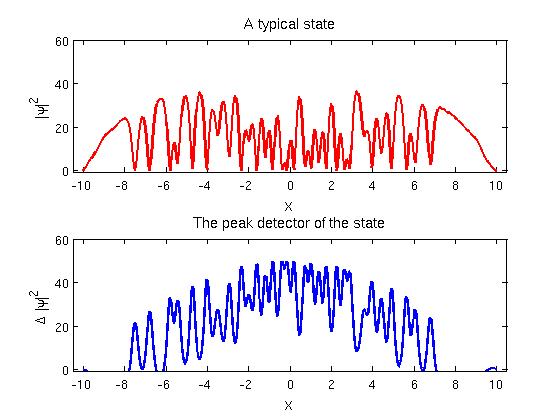
Figure 1: (Color Online) A typical state $|\psi|^{2}$ and dark soliton location detection function $\Delta|\psi|^{2}$ of the BEC with 30 dark solitons during the system’s time evolution. The upper panel is the state $|\psi|^{2}$ and the lower panel is the function $\Delta|\psi|^{2}$ represented by means of a cubic spline interpolation.

II.4 Population annealing Monte Carlo

A state of the system is a list of $\{x_{i}\}$. These wave-particles interact with each other and with the trapping potential. Their dynamics corresponds to an effective one-dimensional lattice, which, in turn, enables us to utilize statistical mechanics techniques. We are going to use a Monte Carlo (MC) method to simulate the system. To work in the same state space, we have therefore integrated out the kinetic energy of the system. The energy function of the system for the MC simulation thus comes only from the potential energy. Therefore the temperature should be of the same scale as the potential energy per particle. Then the transition in temperature should be analogous to the transition in kinetic energy.

We initialize the system from the equilibrium positions, although this is not necessary. We would like to mention here that it is not necessary to know the lattice constant from the mathematical set up to perform the MC simulation. Similarly to the ODE simulation, all we need is the form of the inter-particle potentials. The lattice constant can be estimated from the MC method by looking at states at the lowest temperature. In this way, we obtained the value of 0.3872 from the MC method for the lattice constant compared with the value of 0.3829 of the steady state computation of the ODE problem. The two results agree very well. We use our MC lattice constant to compute $m$ (so as to make the MC simulation more self-consistent/self-contained). The state space of the system is continuous, so it is important to know how to update the state of the system. After some tests with a simple harmonic oscillator, we find that the following MC update method is efficient in the present setting.

• Propose a move of random length with a random direction.
  We can use a random number in the interval $[-h,h]$, where h is a step length and $h>0$, to propose a move to a particle. If the number is positive, then the move is to the right, while if it is negative, the move is to the left.

• Update the state using the Metropolis algorithm.
  We use the Metropolis algorithm in our simulation, i.e., we compute the energy change of $dE$ and accept the move with probability $p=\min[1,e^{-\beta dE}]$. Here $\beta$ is the inverse temperature and is related to temperature $T$ as $\beta=\frac{1}{T}$. In addition, a move is practically rejected if it proposes a swap between two particles since the interaction between them is strongest when they are on top of each other even for the highest temperatures in the simulation. This is not necessary for the thermodynamics of the system, but can nevertheless better reflect the dynamics of the system and also simplify the relevant implementation.

In this work, we use $h=1$. We propose the elementary move to all particles sequentially. A Monte Carlo sweep is an update of the elementary moves for all $N$ particles at once. We will use Monte Carlo sweeps to quantify the amount of work we did in our simulations.

Having introduced how to perform a Monte Carlo sweep at an arbitrary temperature, we now introduce the population annealing Monte Carlo algorithm. This algorithm was introduced in F . It is an example of sequential Monte Carlo A , in contrast to the Markov chain Monte Carlo (MCMC). It is related to simulated annealing, but does annealing with resampling to stay in thermal equilibrium. PAMC has recently been developed and shown to be an efficient algorithm for systems with complicated energy landscapes like spin glasses TBC ; pamc . In this work, we find that PAMC is also efficient for the classical Toda lattice model. The main advantage of PAMC over the simple MC is that PAMC can more accurately maintain thermal equilibrium even for systems with complicated energy landscapes and thermodynamic quantities at multiple temperatures, often a few hundred, can be obtained in a single run. Also, PAMC can be readily done with parallel computing. In fact, in our work, we used OpenMP for the MC simulation implementation.

The PAMC algorithm works as follows:

1. Initialization: Start with $R_{0}$ independent replicas. Choose $N_{T}$ temperatures. The highest temperature for spin glasses is often chosen as $\beta=0$. Here, we start from a finite but high temperature. In this way, we can initialize the particles at the equilibrium positions and do some MC sweeps to start the population at thermal equilibrium. In our simulation, we start at $T=5$ with 40 sweeps for each replica and go down to $T=0.1$, where the particles are ordered. PAMC works by decreasing the temperature slowly from a high temperature to a low temperature following an annealing schedule. Here, we use a schedule of even spacing in $\beta$.

2. Resampling: Suppose we are lowering the temperature from $\beta$ to $\beta^{{}^{\prime}}$, where $\beta^{{}^{\prime}}>\beta$. The re-weighting factor of replica $i$ with energy $E_{i}$ is proportional to $e^{-(\beta^{{}^{\prime}}-\beta)E_{i}}$ and the expected number of copies of replica $i$ is given by

   $$\rho_{i}(\beta,\beta^{{}^{\prime}})=\dfrac{e^{-(\beta^{{}^{\prime}}-\beta)E_{i}}}{Q(\beta,\beta^{{}^{\prime}})},$$ (14)

   where Q is just the sum of all the re-weighting factors, divided by $R_{0}$ to make the sum of $\rho_{i}$ equal to $R_{0}$.

   $$Q(\beta,\beta^{{}^{\prime}})=\frac{\sum\limits_{i=1}^{R}e^{-(\beta^{{}^{\prime}}-\beta)E_{i}}}{R_{0}}.$$ (15)

   The number of replicas can be fixed to a constant by using the multinomial distribution B or the residual resampling method math . We can also allow the population size to fluctuate. For example, we can choose the number of copies for replica $i$ from a Poisson distribution B or the nearest integer distribution. Here we use the nearest integer resampling method, which has the smallest variance. Let the integer part of $\rho_{i}$ be $k_{i}$. The number of copies $n_{i}$ of replica $i$ is either $k_{i}+1$ with probability $\rho_{i}-k_{i}$ or $k_{i}$ with probability $1-(\rho_{i}-k_{i})$. Note that the expectation value of $n_{i}$ is $\rho_{i}$.

3. MCMC sweeps: Because the new population is now more correlated, since some of the replicas are the same due to duplications and also for the purpose of ergodicity to fully explore the phase space, since the population size is finite, we do $N_{S}$ MCMC sweeps to all replicas using the Metropolis algorithm after the resampling step.

4. Repeat step 2 and step 3 $N_{T}-1$ times to go from the highest temperature to the lowest temperature.

The parameters of the MC simulation of the 30 dark solitons are: $R_{0}=5\times 10^{4},\ N_{T}=301$ and $N_{S}=10$. Having passed the equilibrium criteria of TBC , we believe that we have equilibrated the system at all temperatures.

III Dark-bright solitons

III.1 The coupled GPE model and the particle picture

As indicated also in the Introduction, dark-bright soliton (DBS) states are interesting non-linear structures on top of the BEC background for the one dimensional two-component BECs. As such, these states have also undergone intense theoretical investigation; see e.g. buschanglin ; DDB ; kanna ; rajendran ; val ; berloff ; VB ; Alvarez ; vaspra ; vasnjp ; fot for a number of relevant studies. The prototypical one-dimensional model where such states can be found to arise is the coupled GPE peter2 of the form:

$$i{\psi_{j}}_{t}=-\frac{1}{2}{\psi_{j}}_{xx}+\frac{1}{2}\omega^{2}x^{2}{\psi_{j}}+(|\psi_{1}|^{2}+|\psi_{2}|^{2})\psi_{j}-\mu_{j}\psi_{j},\ j=1,2$$ (16)

where $\psi_{j}\in\mathbb{C}$ is a complex field of the component $j$ defined on $(x,t)\in(\mathbb{R},\mathbb{R})$ and $\mu_{j}$ is the chemical potential related to the total number of particles of the component $j$ in the BEC, while $\omega$ is the frequency of the trapping potential. Here, we have also assumed a scattering length setting akin to that the case of ⁸⁷Rb where the near equality of self- and cross- scattering lengths makes it a reasonable first order approximation to assume that all the nonlinear prefactors are equal.

A similar transformation can be done to the coupled GPE equation, as per the discussion of peter2 . Here, on top of the (inverted parabola) ground state, we can “baptize” DB solitons of the form:

$$u_{1}(\xi,\tau) = \cos\phi\tanh\{D[\xi-\xi_{0}(\tau)]\}+i\sin\phi$$ (17)

$$u_{2}(\xi,\tau) = \eta{\rm{sech}}\{D[\xi-\xi_{0}(\tau)]\}e^{ik\xi+i\theta(\tau)}.$$ (18)

In the unperturbed (e.g., by the parabolic trap) problem the parameters satisfy the following relations

$$D^{2} = \cos\phi^{2}-\eta^{2}$$ (19)

$$\dot{\xi_{0}} = k=D\tan\phi$$ (20)

$$\theta(\tau) = \frac{1}{2}(D^{2}-k^{2})\tau+(\tilde{\mu}-1)\tau,$$ (21)

where $\tilde{\mu}=\mu_{2}/\mu_{1}$. As before, far from the linear limit, in the so-called Thomas-Fermi regime, we can multiply particle-like dark soliton states to the ground state to get the first component (approximate) wavefunction. In the second component, we correspondingly add bright soliton states (located at the same spot as the dark solitons), possibly with a phase difference $e^{i\Delta\theta}$ between adjacent waves. A general state with $s$ dark-bright solitons located at $\{a_{i}\}$ with dark soliton phase angles $\{\phi_{i}\}$ and bright soliton amplitudes $\{\eta_{i}\}$ can therefore be written in the following form

$$\psi_{1} = \sqrt{\mu_{1}-V}\prod_{j=1}^{s}\{\cos\phi_{j}\tanh\{D_{j}[\xi-a_{j}(\tau)]\}$$ (22)

$$+ i\sin\phi_{j}\}$$

$$\psi_{2} = \sum_{j=1}^{s}\eta_{j}{\rm{sech}}\{D_{j}[\xi-a_{j}(\tau)]\}e^{ik_{j}\xi+i\theta_{j}(\tau)}e^{i\Delta\theta j}.$$ (23)

If $\Delta\theta=0$ between adjacent waves, the bright solitons are in phase, while if $\Delta\theta=\pi$ between them, we say the bright solitons are out of phase. The interaction energy between a pair of identical static dark-bright solitons has been recently derived in peter2 . More specifically, it was indentified in that work that $U_{DBS}=U_{DD}+2U_{DB}+U_{BB}$, where the three terms stand for dark-dark soliton same-component interaction, dark-bright soliton inter-component interaction and bright-bright soliton same-component interaction respectively. Here, we summarize the kinetic energy for the PDE simulation and the potential energy for the ODE and MC simulations in real space for the dark-bright solitons peter2 .

$$E_{k} = \frac{1}{2}\mu_{1}k^{2}$$ (24)

$$V(x) = \frac{1}{2}\omega_{os}^{2}x^{2}$$ (25)

$$U_{DD} = \frac{1}{\chi_{0}}\left(\frac{272-176D_{0}^{2}}{3D_{0}}+32(D_{0}^{2}-1)(r+\frac{1}{2D_{0}})\right)$$ (26)

$$\times e^{-2D_{0}r}$$

$$U_{BB} = \frac{\chi}{\chi_{0}}\left(-6D_{0}-2\chi+2D_{0}^{2}(r+\frac{1}{D_{0}})\right)$$ (27)

$$\times D_{0}\cos(\Delta\theta)e^{-D_{0}r}+\frac{\chi^{2}}{\chi_{0}}(1+2\cos^{2}\Delta\theta)$$

$$\times \left(3-2D_{0}(r+\frac{1}{2D_{0}})\right)D_{0}e^{-2D_{0}r}$$

$$U_{DB} = \frac{\chi}{\chi_{0}}8\cos(\Delta\theta)e^{-D_{0}r}$$ (28)

$$+ \frac{\chi}{\chi_{0}}\left(-\frac{104}{3}+16D_{0}(r+\frac{1}{2D_{0}})\right)e^{-2D_{0}r},$$

where $\omega_{os}^{2}=\omega^{2}\left(\frac{1}{2}-\frac{\chi}{\chi_{0}}\right)$. $D_{0}$ is the value of $D$ for the static dark-bright solitons, $\chi=\frac{2\eta^{2}}{D_{0}}$ and $\chi_{0}=8\sqrt{1+\left(\frac{\chi}{4}\right)^{2}}$. $r$ is the distance between the two adjacent dark-bright solitons. We can also define the average initial kinetic energy per DBS, $e_{k}$. It is clear that the interaction of the DBSs is much more complicated than that of the single-component dark solitons. The interaction depends on the amplitudes of the bright solitons via $\chi$. Therefore, to perform the relevant simulations using the particle picture, we need some input of the parameters of $\eta$ of each bright soliton. We extract this information from the numerical stationary DBS state. We can optimize the unknown parameters of the particle state by minimizing the norm of the difference of the particle state and the numerical stationary state. Therefore, we will first talk about an effective procedure to obtain multi-DBS stationary states in the next section.

III.2 Identification and continuation of stationary DBS states

We trace stationary states of DBSs using Newton’s method, applied to the corresponding steady state problem of Equations (16). A key to the convergence in this regard is a suitable initialization of the fixed point algorithm. There are two chemical potentials in the equation. The idea of continuation from the linear limit is to couple a state $|n\rangle$ and $|0\rangle$ for the in-phase DBS from the linear limit of quantum harmonic oscillator. For out-of-phase DBS states, we can couple the linear states $|n\rangle$ and $|n-1\rangle$. With the starting chemical potentials suitably chosen slightly above the linear limit, a continuation of the relevant states in the chemical potentials can be performed. A few examples of both in-phase and out-of-phase DBS stationary states are shown in Figure 2 and  3 respectively. The few DBS states are in line with the states reported in peter2 , while a discussion of DBS consisting of many waves and possible analytical DBS-lattice solutions based on elliptic functions are given in tsitoura .

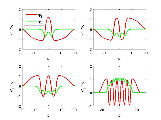
Figure 2: (Color Online) A few in phase DBS states. For the two (top left), three (top right) and four (bottom left) dark-bright soliton states, $\mu_{1}=1.5,\ \mu_{2}=1$. For the ten dark-bright soliton states (bottom right), $\mu_{1}=2.25,\ \mu_{2}=1.5$.

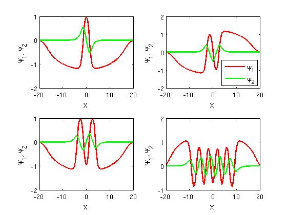
Figure 3: (Color Online) A few out of phase DBS states in a similar format as in the previous figure. For the two, three and four dark-bright soliton states, $\mu_{1}=1.5,\ \mu_{2}=1$. For the ten dark-bright soliton states, $\mu_{1}=1.8,\ \mu_{2}=1.5$.

III.3 Order parameter and simulation methods

From the stationary multi-DBS state, we can clearly discern that the amplitudes of the bright solitons at the edges are somewhat smaller than those around the center. This renders the measurement of the bright soliton locations more challenging, especially during the time evolution process. In this work, we only measure the locations of the dark solitons similarly to what we did in Section II.3 but now with a somewhat smaller cut-off of $\Delta|\psi|^{2}>0.5$. Then, we can extend the order parameter of single component dark solitons to the case of dark-bright solitons too. However, to confirm the genuine two-component nature of the observed dynamics, we have checked carefully that bright solitons are indeed following their dark soliton siblings in our simulations. We will discuss this further in section IV.2. To be able to more clearly identify bright solitons, we chose to simulate the out-of-phase dark-bright soliton system. For the PDE simulation, each bright soliton was initialized with the best fit amplitudes. For the ODE and MC simulations, things are a bit more complicated since the interaction potentials of Equations (26)-(28) apply only to equal amplitude DBS pairs. Therefore, we have made an approximation by using the average of the best fit amplitudes of all bright solitons for each bright soliton in the ODE and PAMC simulations. This naturally introduces some error, but we have systematically checked that this doesn’t substantially affect our results. For example, we computed the lattice constants using ODE and PAMC and found that they agree reasonably well with the PDE lattice constant. The PDE lattice constant is 2.07 while the ODE lattice constant is 2.10 and the PAMC lattice constant is found to be 2.13. We used each method’s lattice constant for the respective simulations to compute the order parameter in a self-consistent fashion. Moreover, we have also carefully checked that for the same disorder realization, our ODE simulation can well capture the PDE dynamics. This will also be discussed in section IV.2.

Finally, we briefly summarize our simulation parameters for the DBS simulation. For the PDE simulation, we used $\mu_{1}=1.8,\ \mu_{2}=1.5,\ N=10,\ \omega=0.1,\ dx=0.05,\ dt=0.002,\ t=200.$ The reason for using different trapping frequencies for the two separate settings of dark and dark-bright solitary waves is because we are following the parameters of the original works focusing, respectively, on them in DS1 ; peter2 . In this way, we can benchmark some of our results against the original papers whenever possible, e.g., as concerns the all-in-phase soliton oscillation frequencies, stationary states, equilibrium positions etc. In any event, as mentioned previously this is simply a matter of scaling of length scales and should not affect our main results. For each sample, we record $e_{k}$ and measure the state and the order parameter $m$ over each time period 1. Again, our ODE parameters are the same except for $dt=0.01$ and we also record our states over each time period 0.01 for the ODE simulation. In our PAMC simulation, we used $R_{0}=5\times 10^{4},\ N_{T}=101$ and $N_{s}=10$. We checked that our simulation again passed the equilibrium criteria of TBC . Having presented the general framework, we now turn to a systematic reporting of the relevant results.

IV Results

IV.1 One component dark solitons

The main scope of our study concerns the examination of how the order parameter changes as a function of our kinetically defined temperature. Figure 4 shows how the order parameter changes with $T$. Here we have generalized our notation of $T$ to stand for temperature for the MC method and for average initial kinetic energy per particle for the ODE and PDE simulations. Since the two quantities should have the same scale, this justifies the use of the same notion for simplicity. We will refer to this quantity as “kinetic temperature”. We can see that the order parameter features a monotonic decay as $T$ grows. It is interesting to see that the three different methods (PDE, ODE and PAMC) agree reasonably well with each other in predicting this fundamental trait. There is a gradual transition between the ordered phase and the disordered phase with an energy scale of about 1 (in our dimensionless units). This suggests the existence of a modification of the system’s behavior from a highly ordered one (near unity values of $m$) to a quite disordered one (values of $m$ around or below $0.1$). This transition seems to be smooth and gradual and does not feature the characteristics of standard thermodynamic phase transitions. This indeed may be reasonable to expect in our 1d system, although whether such genuine transitions may exist for different solitonic multi-particle states e.g. in higher dimensions remains a question worth exploring.

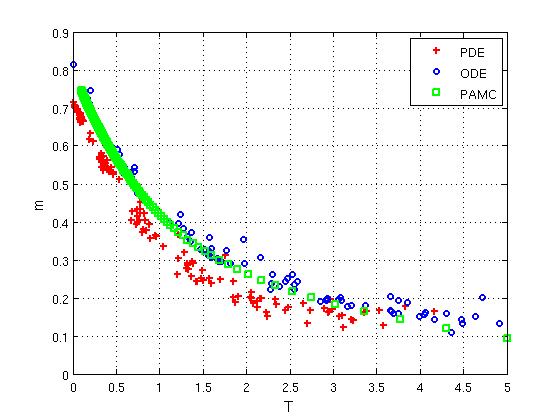
Figure 4: (Color Online) The monotonically decreasing behavior of the order parameter as a function of our kinetically defined $T$ for the dark soliton system.

The three different regimes of the dark solitons are clearly discernible in our simulations: there exists the ordered phase, the transition (intermediate) phase and the disordered phase. So it is interesting to know what the typical dynamics look like in each of these three different regimes. Figure 5 shows three typical time evolutions of the dark solitons in these respective regimes from the PDE simulation. A similar result but from the ODE simulation is shown in Figure 6. It is clear from the PDE figure that in the ordered regime, the dark solitons don’t cross each other. In the transition regime, they start to cross each other once in a while. In the disordered regime, they do crossing frequently. In this case, the highly energetic (both in the PDE and in the ODE) soliton particles resemble those of a “gas”.

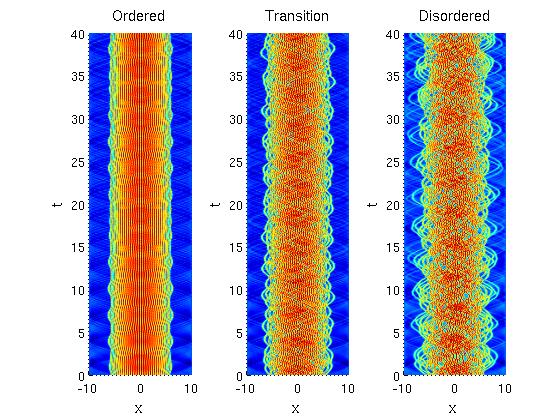
Figure 5: (Color Online) Typical dynamics of the dark solitons in the ordered, transition (intermediate) and disordered regimes as captured by case examples of the PDE simulation.

Figure 6: (Color Online) Typical dynamics of the dark solitons in the ordered, transition (intermediate) and disorder regimes, as illustrated within the ODE simulation.

IV.2 Dark-bright solitons

Here we show similar results of how the order parameter changes as our kinetic temperature increases for the DBSs. Figure 7 shows how the order parameter changes with $T$. There is again a gradual transition between the ordered phase and the disordered phase with an energy scale of about 0.05 for the parameters selected here. Once again, the overall trend of the PDE and ODE, as well as the PAMC is fairly similar. Nevertheless, the PDE seems to be somewhat less ordered than the other two, conceivably because of the enhanced role of the additional degrees of freedom and the more complex nature of the associated dynamics in this two-component setting. Some typical PDE and ODE ordered, transition (i.e., intermediate) and disordered states are shown in Figures 8, 9, 10 and 11.

We also want to point out here that Figure 9 and Figure 10 are worth commenting upon further in that some of the bright solitons seem to be less visible due to the highly collisional nature of the dynamics. We therefore checked the dynamical stability of the stationary dark-bright soliton state. In accordance with the results of tsitoura , we found there is some instability but nevertheless the corresponding growth rate is rather small, i.e., small enough that over the time scales reported herein, the resulting weak dynamical instabilities (of stationary states) have not yet set in. Our detailed examination of this feature suggests that during the intermediate, as well as disordered phase dynamics, the collisional dynamics may develop high amplitudes, thus rendering some of the bright solitons less visible in the space-time plots of e.g. 9 and 10. To shed further light on this issue, we have looked at the peaks of the dark (after being subtracted from the ground state background) and bright soliton components. The result of the same states as Figure 9 is shown in Figure 12, which clearly attests to the fact that the bright solitons are indeed following suit with respect to their dark soliton partners. Similar results are obtained for states in other disorder realizations. Nevertheless, this phenomenology of amplitude enhancement and apparent “mass exchange” may be worth exploring further and may be, in part, related to (a generalization of) the two DBS self-trapping phenomenology recently reported in karamatskos .

Finally, it is interesting to check whether the ODE simulation can match the peaks in the PDE simulation for the same disorder realization. A typical result of the ODE and PDE simulation of the same disorder realization as Figure 9 with the same initial kinetic energy is shown in Figure 13. We have shown the trajectories of the dark-bright solitons of the ODE simulation on the left panel and the dark soliton component of the PDE simulation on the right panel. It is clear from the figure that even though we have made some approximations for the particle interactions, the ODE simulation nevertheless captures fairly accurately the dynamics of the full PDE simulation. Similar results were found for dark-bright solitons in other regimes and also for the simpler case involving solely dark solitons.

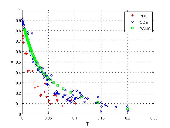
Figure 7: (Color Online) The monotonically decreasing dependence of the order parameter as a function of our kinetically defined $T$ for the DBS system.

Figure 8: (Color Online) Typical dynamics of the ordered state for the DBS system, resulting from the PDE simulation. The space-time evolution of the field is shown in the two components.

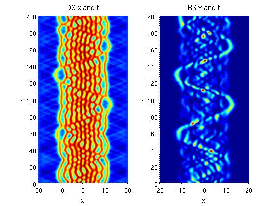
Figure 9: (Color Online) Typical dynamics of the transition (intermediate) state for the DBS system, from the PDE simulation.

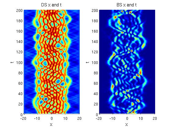
Figure 10: (Color Online) Typical dynamics of the disordered state for the DBS system, again showing both components space-time evolution from the PDE simulation.

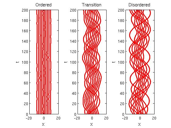
Figure 11: (Color Online) Typical dynamics of the ordered, transition and disordered states for the DBS system, as resulting from the ODE simulation.

Figure 12: (Color Online) The same states as 9, but instead of showing density, we plotted the peaks of the states from the dark (left) and bright (right) components.

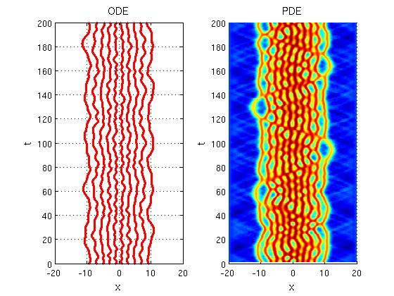
Figure 13: (Color Online) The same states as 9, but the left panel is now the ODE simulation with the same disorder realization as the corresponding PDE simulation. The dark soliton component is shown on the right panel. The two simulations have the same initial kinetic energy. Note that the ODE can accurately capture the PDE dynamics.

V Conclusions and Future Challenges

In the present work, we did a systematic numerical simulation of the states of the one-dimensional dark soliton and dark-bright soliton lattices in the large density limit using PDE, ODE and PAMC simulations. We identified regimes where the dynamics, as characterized both by a concrete, yet empirical, order parameter and by a direct inspection of the space-time evolution appears ordered, as well as ones where it appears highly disoredered and also monitored intermediate (“transitional”) regimes between these two. The three methods of our numerical choice gave similar results, verifying the good agreement between our different dynamical descriptions. For our defined order parameter, we found that it continuously decreases when our kinetically defined temperature parameter increases. Nevertheless, in our current formulation of the problem and although the different end states for low and high kinetic energy can be considered as “soliton crystals” and “soliton gases”, respectively, no genuine phase transitions were identified in our one-dimensional, one- and two-component formulations.

Our analysis poses a number of interesting questions for future study. One such concerns whether a more rigorous (or numerically assisted) characterization of the thermodynamic properties can be provided for our effective wave-particle system via e.g. the transfer integral method ti1 ; ti2 . For instance, in the dark soliton case, the effective particle system is a perturbed form of a Toda lattice, while for the classical (integrable) Toda lattice, transfer integral based techniques have been used to compute the partition function and thermodynamic quantities, e.g., in ti3 ; ti4 . The use of such techniques even in a numerical form could provide a definitive answer in the question as to whether phase transitions may or may not exist in the present setting. Additionally, it would be particularly interesting to generalize relevant considerations to higher dimensional settings. In particular, a similar effective description can be formulated in the case of a gas of trapped vortices in quasi-2d BECs, where a reduced particle description in the large density limit is also available; see e.g. DS2d . Thus, once again, the use of suitable order parameters can be used to identify the thermodynamics properties of the relevant vortex cloud. These questions are currently under consideration and will be reported in future studies.

- (1) C.J. Pethick and H. Smith, Bose-Einstein Condensation in Dilute Gases, Second Edition, Cambridge University Press (Cambridge, 2008).
- (2) L.P. Pitaevskii and S. Stringari, Bose-Einstein Condensation, Oxford University Press (Oxford, 2003).
- (3) P.G. Kevrekidis, D.J. Frantzeskakis, and R. Carretero-González (eds.), Emergent Nonlinear Phenomena in Bose-Einstein Condensates. Theory and Experiment, Springer-Verlag (Berlin, 2008).
- (4) K.E. Strecker, G.B. Partridge, A.G. Truscott, and R.G. Hulet, Nature 417, 150 (2002).
- (5) L. Khaykovich, F. Schreck, G. Ferrari, T. Bourdel, J. Cubizolles, L.D. Carr, Y. Castin, and C. Salomon, Science 296, 1290 (2002).
- (6) S.L. Cornish, S.T. Thompson, and C.E. Wieman, Phys. Rev. Lett. 96, 170401 (2006).
- (7) B. Eiermann, Th. Anker, M. Albiez, M. Taglieber, P. Treutlein, K.-P. Marzlin, and M.K. Oberthaler, Phys. Rev. Lett. 92, 230401 (2004).
- (8) D.J. Frantzeskakis, J. Phys. A 43, 213001 (2010).
- (9) A.L. Fetter and A.A. Svidzinsky, J. Phys.: Condens. Matter 13, R135 (2001).
- (10) A.L. Fetter, Rev. Mod. Phys. 81, 647 (2009).
- (11) S. Komineas, Eur. Phys. J.- Spec. Topics 147 133 (2007).
- (12) S. Burger, K. Bongs, S. Dettmer, W. Ertmer, K. Sengstock, A. Sanpera, G.V. Shlyapnikov, and M. Lewenstein, Phys. Rev. Lett. 83, 5198 (1999).
- (13) J. Denschlag, J.E. Simsarian, D.L. Feder, C.W. Clark, L.A. Collins, J. Cubizolles, L. Deng, E.W. Hagley, K. Helmerson, W.P. Reinhardt, S.L. Rolston, B.I. Schneider, and W.D. Phillips, Science 287, 97 (2000).
- (14) Z. Dutton, M. Budde, C. Slowe, and L.V. Hau, Science 293, 663 (2001).
- (15) K. Bongs, S. Burger, S. Dettmer, D. Hellweg, J. Arlt, W. Ertmer, and K. Sengstock, C.R. Acad. Sci. Paris 2, 671 (2001).
- (16) P. Engels and C. Atherton, Phys. Rev. Lett. 99, 160405 (2007).
- (17) C. Becker, S. Stellmer, P. Soltan-Panahi, S. Dörscher, M. Baumert, E.-M. Richter, J. Kronjäger, K. Bongs, and K. Sengstock, Nature Phys. 4, 496 (2008).
- (18) S. Stellmer, C. Becker, P. Soltan-Panahi, E.-M. Richter, S. Dörscher, M. Baumert, J. Kronjäger, K. Bongs, and K. Sengstock, Phys. Rev. Lett. 101, 120406 (2008).
- (19) A. Weller, J.P. Ronzheimer, C. Gross, J. Esteve, M.K. Oberthaler, D.J. Frantzeskakis, G. Theocharis, and P.G. Kevrekidis, Phys. Rev. Lett. 101, 130401 (2008).
- (20) G. Theocharis, A. Weller, J.P. Ronzheimer, C. Gross, M.K. Oberthaler, P.G. Kevrekidis, and D.J. Frantzeskakis, Phys. Rev. A 81, 063694 (2010).
- (21) I. Shomroni, E. Lahoud, S. Levy and J. Steinhauer, Nat. Phys. 5, 193 (2009).
- (22) Z. Chen, M. Segev, T. H. Coskun, D. N. Christodoulides, Yu. S. Kivshar, and V. V. Afanasjev, Opt. Lett. 21, 1821 (1996).
- (23) E. A. Ostrovskaya, Yu. S. Kivshar, Z. Chen, and M. Segev, Opt. Lett. 24, 327 (1999).
- (24) Z. Chen, M. Segev, T. H. Coskun, D. N. Christodoulides and Yu. S. Kivshar, J. Opt. Soc. Am. B 14, 3066-3077 (1997).
- (25) C. Becker, S. Stellmer, P. Soltan-Panahi, S. Dörscher, M. Baumert, E.-M. Richter, J. Kronjäger, K. Bongs, and K. Sengstock, Nature Phys. 4, 496 (2008).
- (26) S. Middelkamp, J. J. Chang, C. Hamner, R. Carretero-González, P. G. Kevrekidis, V. Achilleos, D. J. Frantzeskakis, P. Schmelcher, and P. Engels, Phys. Lett. A 375, 642 (2011).
- (27) C. Hamner, J. J. Chang, P. Engels, M. A. Hoefer, Phys. Rev. Lett. 106, 065302 (2011).
- (28) D. Yan, J. J. Chang, C. Hamner, P. G. Kevrekidis, P. Engels, V. Achilleos, D. J. Frantzeskakis, R. Carretero-González, and P. Schmelcher, Phys. Rev. A 84, 053630 (2011).
- (29) M. A. Hoefer, J. J. Chang, C. Hamner, and P. Engels, Phys. Rev. A 84, 041605 (2011).
- (30) D. Yan, J. J. Chang, C. Hamner, M. A. Hoefer, P. G. Kevrekidis, P. Engels, V. Achilleos, D. J. Frantzeskakis, and J. Cuevas, J. Phys. B 45, 115301 (2012).
- (31) F. Mitschke, I. Halama, A. Schwache, Chaos Solitons Fractals 10 9113 (1999).
- (32) H. Tercas, D.D. Solsynshkov and G. Malpuech, Phys. Rev. Lett. 110, 035303 (2013).
- (33) G.A. El, A.M. Kamchatnov, Phys. Rev. Lett. 95, 204101 (2005).
- (34) G.A. El, A.L. Krylov, S.A. Molchanov, S. Venakides, Phys. D 152/153, 653 (2001).
- (35) V.E. Zakharov, Stud. Appl. Math. 122, 219 (2009).
- (36) M. Schmidt, S. Erne, B. Nowak, D. Sexty, T. Gasenzer, New J. Phys. 14, 075005 (2012).
- (37) M.P. Coles, D.E. Pelinovsky, and P.G. Kevrekidis, Nonlinearity 23, 1753 (2010).
- (38) D. Yan, F. Tsitoura, P.G. Kevrekidis, D.J. Frantzeskakis, arXiv:1402.1895.
- (39) R. Douc and O.Cappé, In Proc. of the 4th International Symposium on Image and Signal Processing and Analysis (ISPA), pp. 64, IEEE (2005).
- (40) K. Hukushima and Y. Iba, In James E. Gubernatis (Ed.), The Monte-Carlo method in the physical sciences: Celebrating the 50th Anniversary of the Metropolis Algorithm, vol. 690, pp. 200. AIP (2003).
- (41) J. Machta, Phys. Rev. E 82, 026704 (2010).
- (42) J. Machta and R. Ellis, J. Stat. Phys. 144, 541 (2011).
- (43) W. Wang, J. Machta, H.G. Katzgraber, Phys. Rev. B 90, 184412 (2014).
- (44) W. Wang, J. Machta, H.G. Katzgraber, Population annealing for large scale spin glass simulations, in preparation (2014).
- (45) Th. Busch and J. R. Anglin, Phys. Rev. Lett. 87, 010401 (2001).
- (46) H. E. Nistazakis, D. J. Frantzeskakis, P. G. Kevrekidis, B. A. Malomed, and R. Carretero-González, Phys. Rev. A 77, 033612 (2008).
- (47) M. Vijayajayanthi, T. Kanna, and M. Lakshmanan, Phys. Rev. A 77, 013820 (2008).
- (48) S. Rajendran, P. Muruganandam, M. Lakshmanan, J. Phys. B 42, 145307 (2009).
- (49) V. A. Brazhnyi and V. M. Pérez-García, Chaos, Solitons Fractals 44, 381 (2011).
- (50) C. Yin, N. G. Berloff, V. M. Perez-Garcia, V. A. Brazhnyi, and H. Michinel, Phys. Rev. A 83, 051605 (2011).
- (51) K. J. H. Law, P. G. Kevrekidis, and L. S. Tuckerman, Phys. Rev. Lett. 105, 160405 (2010).
- (52) A. Álvarez, J. Cuevas, F. R. Romero, and P. G. Kevrekidis, Physica D 240, 767 (2011).
- (53) V. Achilleos, P. G. Kevrekidis, V. M. Rothos, and D. J. Frantzeskakis, Phys. Rev. A 84, 053626 (2011).
- (54) V. Achilleos, D. Yan, P. G. Kevrekidis, and D. J. Frantzeskakis, New J. Phys. 14, 055006 (2012).
- (55) F. Tsitoura, V. Achilleos, B. A. Malomed, D. Yan, P. G. Kevrekidis, and D. J. Frantzeskakis, Phys. Rev. A 87, 063624 (2013).
- (56) E.T. Karamatskos, J. Stockhofe, P.G. Kevrekidis, P. Schmelcher, arXiv:1411.3957.
- (57) J.A. Krumhansl and J.R. Schrieffer, Phys. Rev. B 11, 3535 (1974).
- (58) S. Aubry, J. Chem. Phys. 62, 3217 (1975).
- (59) H. Büttner and F.G. Mertens, Solid State Commun. 29, 663 (1979).
- (60) F.G. Mertens and H. Büttner, Phys. Lett. 84A, 335 (1981).
- (61) D.E. Pelinovsky and P.G. Kevrekidis, Nonlinearity 24, 1271 (2011).