Cosmological particle creation in a hadronic fluid

Abstract

Acoustic perturbations in an expanding hadronic fluid at temperatures below the chiral transition point represent massless pions propagating in curved spacetime geometry. In comoving coordinates the corresponding analog metric tensor describes a hyperbolic Friedmann-Robertson-Walker (FRW) spacetime. We study the analog cosmological particle creation of pions below the critical point of the chiral phase transition. We compare the cosmological creation spectrum with the spectrum of analog Hawking radiation at the analog trapping horizon.

I Introduction

Quantum field theory in a curved spacetime predicts that the gravitation field creates particles and antiparticles. The main related phenomena are the Hawking effect in black holes and particle creation due to the cosmological expansion parker1 . In the latter case the creation is caused by the time dependence of the background metric which in turn causes a nontrivial time evolution of the ground state similar to what happens to a quantum harmonic oscillator with time-dependent frequency jacobson1 . The process of particle creation depends only on the particulars of the metric and particle properties (mass, spin etc.) irrespective of whether the expansion is of cosmological or another origin. In particular, particle creation is expected in time-dependent analog gravity systems such as expanding Bose-Einstein (BE) condensates barcelo1 ; jain ; kurita ; sabin , Bose and Fermi superfluids fedichev , and expanding hadronic fluids tolic ; tolic2 .

Analog gravity has proven to be useful in studying various physical phenomena barcelo , e.g., acoustics visser , optics philbin , superfluidity jacobson2 , black hole accretion moncrief ; abraham , and hadron fluid tolic ; tolic2 ; tolic3 . The purpose of this paper is to study in the framework of analog gravity the phenomenon of cosmological particle creation in a hadronic fluid produced in high energy collision experiments.

Strongly interacting matter is described at the fundamental level by a non-Abelian gauge theory called quantum chromodynamics (QCD). At low energies, the QCD vacuum is characterized by a nonvanishing expectation value shifman : $\langle\bar{\psi}\psi\rangle\approx$ (235 MeV)³, theso-called chiral condensate. This quantity describes the density of quark-antiquark pairs found in the QCD vacuum and its nonvanishing value is a manifestation of chiral symmetry breaking harris . Our approach is based on the linear sigma model gell combined with a boost invariant Bjorken-type spherical expansion lampert . The linear sigma model serves as an effective model for the low-temperature phase of QCD bilic ; bilic1 . In the chirally broken phase, i.e., at temperatures below the point of the chiral phase transition, the pions are massless but owing to the finite temperature effects propagate slower than light pisarski ; son1 ; son2 . Moreover, the pion velocity approaches zero at the critical temperature.

As in general relativity, a notable manifestation of analog gravity are two effects both having a quantum origin: the Hawking radiation and cosmological particle creation. These two phenomena are similar but appear under different physical conditions. The Hawking thermal radiation is due to the information loss across the apparent horizon whereas the cosmological particle creation generates a quasithermal radiation as a result of time variation of the spacetime geometry. The Hawking radiation takes place only if there exists a trapping (or apparent) horizon, whereas the cosmological particle creation takes place with or without a horizon. On the other hand, in any stationary geometry the cosmological particle creation is absent whereas the Hawking radiation is present in a stationary geometry with an event horizon. Besides, if a field theory is conformally invariant there will be no cosmological particle creation. In contrast, the Hawking radiation is present even in the conformal case as long as a trapping horizon exists.

The analog Hawking effect has been studied in our previous papers tolic ; tolic2 in the context of an expanding hadronic fluid. We have demonstrated that there exists a region where the flow velocity exceeds the pion velocity and the analog trapped region forms which then causes the Hawking radiation of massless pions. Here we study the effect of cosmological creation of pions in an expanding hadronic fluid in terms of the Bogoliubov transformation grib and adiabatic expansion parker1 ; parker3 . For alternative approaches to cosmological particle creation see, e.g., Refs. hamilton ; greenwood .

The remainder of the paper is organized as follows. In Sec. II we describe the analog model based on the expanding chiral fluid. The cosmological particle creation of pions is studied in Sec. III in which we derive the spectrum of the created pions and the time dependence of the particle number. We estimate the temperature by fitting our spectrum to the Planck black body radiation spectrum. In the concluding section, Sec. IV, we summarize our results and discuss physical implications.

II Expanding chiral fluid

In this section we describe the hadron fluid in terms of the linear sigma model at finite temperature undergoing a spherically symmetric expansion. Our model is based on a scalar field Lagrangian with spontaneously broken chiral symmetry which we describe in Sec. II.1. Then in Sec. II.2 we specify the dynamics of the fluid based on the Bjorken expansion model.

II.1 Linear sigma model

Consider a linear sigma model at finite temperature in the Minkowski spacetime background. The background medium is a hadronic fluid consisting of predominantly pions. The dynamics of mesons in such a medium is described by an effective Lagrangian with spontaneously broken chiral symmetry bilic2

$${\cal L}_{\rm eff}= \frac{1}{2}(fg^{\mu\nu}+gu^{\mu}u^{\nu})(\partial_{\mu}\sigma\partial_{\nu}\sigma+\partial_{\mu}\mbox{\boldmath$\pi$}\partial_{\nu}\mbox{\boldmath$\pi$})$$ (1)

$$-\frac{m_{\sigma}^{2}}{2}\sigma^{2}-\frac{m_{\pi}^{2}}{2}\mbox{\boldmath$\pi$}^{2}-U(\sigma,\mbox{\boldmath$\pi$}),$$

where $g^{\mu\nu}$ is the inverse of the background metric. As we are working in units in which $\hbar=c=1$ the velocity of the fluid $u_{\mu}$ is normalized as $g^{\mu\nu}u_{\mu}u_{\nu}=1$.

The coefficients $f$ and $g$ depend on the local temperature $T$ and on the parameters of the sigma model: the coupling constant $\lambda$ and the pion decay constant $f_{\pi}$, and may be calculated in perturbation theory. The scalar fields $\sigma$ and $\pi_{i}$, where $i=1,2,3$, represent fluctuations around the expectation values $\langle\sigma\rangle$ and $\langle\pi_{i}\rangle$, respectively. The expectation values of the pion fields $\langle\pi_{i}\rangle$ are chosen to vanish always whereas the expectation value of the sigma field $\langle\sigma\rangle$, usually referred to as the chiral condensate, is temperature dependent and vanishes at the critical temperature $T_{\rm c}$. The scaling and universality analysis son1 yields $\langle\sigma\rangle\sim(T-T_{\rm c})^{\beta}$ in the vicinity of the critical point. At zero temperature $\langle\sigma\rangle$ is normalized to the pion decay constant, i.e., $\langle\sigma\rangle=f_{\pi}$ at $T=0$. The meson masses depend on temperature and below the chiral transition point are given by

$$m_{\pi}^{2}=0,\quad m_{\sigma}^{2}=2\lambda\langle\sigma\rangle^{2}.$$ (2)

The potential $U$ is

$$U(\sigma,\mbox{\boldmath$\pi$})=\lambda\langle\sigma\rangle\sigma(\sigma^{2}+\mbox{\boldmath$\pi$}^{2})+\frac{\lambda}{4}(\sigma^{2}+\mbox{\boldmath$\pi$}^{2})^{2}.$$ (3)

The temperature dependence of $\langle\sigma\rangle$ is obtained by minimizing the thermodynamic potential $\Omega=-(T/V)\ln Z$ with respect to $\langle\sigma\rangle$ at fixed temperature $T$ bilic1 . The scaling and universality analysis son1 yields $\langle\sigma\rangle\sim(T-T_{\rm c})^{\beta}$ in the vicinity of the critical point with $\beta=0.388$ for the O(4) universality class hasenbusch ; toldin . Furthermore, the extremum condition was solved numerically at one-loop order tolic2 ; bilic1 and the value of the critical temperature $T_{\rm c}=183$ MeV was found with $f_{\pi}=92.4$ MeV and $m_{\sigma}=1$ GeV as a phenomenological input.

The action corresponding to the Lagrangian (1) may be expressed as tolic2

$$S_{\rm eff}= \int d^{4}x\sqrt{-G}\,\left[\frac{1}{2}G^{\mu\nu}(\partial_{\mu}\sigma\partial_{\nu}\sigma+\partial_{\mu}\mbox{\boldmath$\pi$}\partial_{\nu}\mbox{\boldmath$\pi$})\right.$$ (4)

$$\left.-\frac{c_{\pi}}{f^{2}}\left(\frac{m_{\sigma}^{2}}{2}\sigma^{2}+\frac{m_{\pi}^{2}}{2}\mbox{\boldmath$\pi$}^{2}+U(\sigma,\mbox{\boldmath$\pi$})\right)\right],$$

where the effective metric tensor, its inverse, and its determinant are given by

$$G_{\mu\nu}=\frac{f}{c_{\pi}}[g_{\mu\nu}-(1-c_{\pi}^{2})u_{\mu}u_{\nu}],$$ (5)

$$G^{\mu\nu}=\frac{c_{\pi}}{f}\left[g^{\mu\nu}-(1-\frac{1}{c_{\pi}^{2}})u^{\mu}u^{\nu}\right],$$ (6)

$$G\equiv\det G_{\mu\nu}=\frac{f^{4}}{c_{\pi}^{2}}\det g_{\mu\nu}.$$ (7)

with the pion velocity $c_{\pi}$ defined by

$$c_{\pi}^{2}=\frac{f}{f+g}.$$ (8)

It is worth noting that there exists a straightforward map between the metric (5) and the relativistic acoustic metric moncrief ; bilic3 ; visser2

$${\cal G}_{\mu\nu}=\frac{n}{m^{2}wc_{\rm s}}[g_{\mu\nu}-(1-c_{\rm s}^{2})u_{\mu}u_{\nu}]$$ (9)

derived for acoustic perturbations in an ideal relativistic fluid with the adiabatic speed of sound $c_{\rm s}$ defined as

$$c_{\rm s}^{2}=\left.\frac{dp}{d\rho}\right|_{s/n}.$$ (10)

The symbols $n$, $p$, $\rho$ and $w=(p+\rho)/n$ denote, respectively the particle number density, pressure, energy density, and specific enthalpy. The expression (9) compared with the original one bilic3 differs by a factor $1/m^{2}$ which we have introduced here to make the acoustic metric dimensionless. The mapping between $G_{\mu\nu}$ and ${\cal G}_{\mu\nu}$ is achieved by identifying the pion velocity $c_{\pi}$ with the speed of sound $c_{\rm s}$ and the quantity $f$ with $n/(m^{2}w)$. The physical meaning of $f$ may be seen in the nonrelativistic limit in which case $n\rightarrow\rho/m$ and $w\rightarrow m$, and hence, $f\rightarrow\rho/m^{4}$. Thus, in this limit the quantity $f$ is proportional to the energy density $\rho$. At zero temperature the energy density is just the rest mass density, i.e., $\rho|_{T=0}=m/V=m^{4}$ so $f|_{T=0}=1$.

In the absence of the medium (or equivalently at zero temperature) we have $f=1$ and $g=0$. At nonzero temperature, $f$ and $g$ are derived from the finite temperature self-energy $\Sigma(q,T)$ in the limit when the external momentum $q$ approaches zero and can be expressed in terms of second derivatives of $\Sigma(q,T)$ with respect to $q_{0}$ and $q_{i}$. The quantities $f$, $g$, and $c_{\pi}$ as functions of temperature have been calculated at one-loop level by Pisarski and Tytgat in the low temperature approximation pisarski

$$f\simeq 1-\frac{T^{2}}{12f_{\pi}^{2}}-\frac{\pi^{2}}{9}\frac{T^{4}}{f_{\pi}^{2}m_{\sigma}^{2}},\quad g\simeq 1+\frac{8\pi^{2}}{45}\frac{T^{4}}{f_{\pi}^{2}m_{\sigma}^{2}},$$

$$c_{\pi}^{2}\simeq 1-\frac{8\pi^{2}}{45}\frac{T^{4}}{f_{\pi}^{2}m_{\sigma}^{2}},$$ (11)

and by Son and Stephanov for temperatures close to the chiral transition point son1 ; son2 (see also Ref. tolic ). In $d=3$ dimensions one finds

$$f\simeq c_{1}(1-z)^{\nu-2\beta},\quad f+g\simeq c_{2}(1-z)^{-2\beta},$$

$$c_{\pi}^{2}\simeq c_{3}(1-z)^{\nu},$$ (12)

in the limit $z\equiv T/T_{\rm c}\rightarrow 1$. Here $c_{1}$, $c_{2}$, and $c_{3}$ are constants and $\nu=0.749$ and $\beta=0.388$ are the critical exponents for the O(4) universality class hasenbusch ; toldin . Combining this with (11) and the numerical results at one-loop order tolic2 , a good fit in the entire range $0\leq T\leq T_{\rm c}$ is achieved with

$$f=(1-z^{2})^{\nu-2\beta}(1-pz^{2})^{q},\quad c_{\pi}^{2}=(1-z^{4})^{\nu},$$ (13)

where $p$ and $q$ are positive parameters. The constants in (12) are then fixed to $c_{1}=2^{\nu-2\beta}(1-p)^{q}$, $c_{2}=2^{-\nu-2\beta}(1-p)^{q}$ and $c_{3}=2^{2\nu}$. With (13) we capture the main features: with the values $p=0.1$ and $q=3.58$ we match the zero temperature limit pisarski and we recover the correct critical behavior (12).

The variation of the action (4) yields the Klein–Gordon wave equation in curved space

$$\frac{1}{\sqrt{-G}}\,\partial_{\mu}(\sqrt{-G}\,G^{\mu\nu})\partial_{\nu}\varphi+\frac{c_{\pi}}{f^{2}}\left[m_{\varphi}^{2}+V_{\varphi}(\sigma,\mbox{\boldmath{$\pi$}})\right]\varphi=0,$$ (14)

where $\varphi$ stands for $\pi_{i}$ or $\sigma$ and

$$V_{\varphi}(\sigma,\mbox{\boldmath{$\pi$}})=2\frac{\partial U}{\partial\varphi^{2}}$$ (15)

are the corresponding interaction potentials.

II.2 Spherical Bjorken expansion

In this section we will completely specify the analog metric $G_{\mu\nu}$ by fixing the background metric $g_{\mu\nu}$ and the velocity field $u_{\mu}$ and by deriving the spacetime dependence of the quantities $f$ and $c_{\pi}$. So far, $f$ and $c_{\pi}$ are expressed as functions of temperature via (13) and we will see that once we specify the dynamics of the fluid, the spacetime dependence of $f$ and $c_{\pi}$ will follow from their temperature dependence.

To this end we consider a boost invariant Bjorken-type spherical expansion bjorken . This type of expansion has been recently applied to mimic an open FRW metric in a relativistic BE system fagnocchi ; tolic3 . In this model the radial three-velocity in radial coordinates $x^{\mu}=(t,r,\theta,\phi)$ is a simple function $v=r/t$. Then the four-velocity is given by

$$u^{\mu}=(t/\tau,r/\tau,0,0),$$ (16)

where $\tau=\sqrt{t^{2}-r^{2}}$ is the proper time of observers comoving along the fluid worldlines. With the substitution

$$t=\tau\cosh y,$$

$$r=\tau\sinh y,$$ (17)

the four-velocity velocity is expressed as

$$u^{\mu}=(\cosh y,\sinh y,0,0).$$ (18)

The substitution (17) may be regarded as a coordinate transformation from ordinary radial coordinates to new coordinates $(\tau,y,\theta,\phi)$ in which the flat background metric takes the form

$$g_{\mu\nu}={\rm diag}\left(1,-\tau^{2},-\tau^{2}\sinh^{2}\!y,-\tau^{2}\sinh^{2}\!y\sin^{2}\!\theta\right).$$ (19)

Thus, the transformation (17) maps the spatially flat Minkowski spacetime into an expanding FRW spacetime with cosmological scale $a=\tau$ and negative spatial curvature. The resulting flat spacetime with metric (19) is known in cosmology as the Milne universe milne .

The velocity components in this coordinate frame are $u^{\mu}=(1,0,0,0)$, and hence, the new coordinate frame is comoving. Using this and (19) from (5) we obtain the analog metric in a diagonal form

$$G_{\mu\nu}=\left(\begin{array}[]{cccc}b^{2}&&&\\ &-a^{2}&&\\ &&-a^{2}\sinh^{2}\!y&\\ &&&-a^{2}\sinh^{2}\!y\sin^{2}\theta\end{array}\right),$$ (20)

where

$$b=\sqrt{fc_{\pi}},\quad a=\tau\sqrt{\frac{f}{c_{\pi}}}.$$ (21)

This metric is of the form of a FRW spacetimes with negative spatial curvature provided the quantities $f$ and ${c_{\pi}}$ are functions of time only.

We could, in principle, convert the metric (20) back to the original coordinates $(t,r,\theta,\phi)$ using the inverse of the transformation (17) and proceed with calculations in the laboratory frame. However, for our purpose it is advantageous to do the calculations in the comoving reference frame mainly for the following reasons. The original coordinate frame (or laboratory frame) is not suitable for thermodynamic considerations since the thermodynamic variables, such as temperature, are always defined in the fluid rest frame or the comoving frame. Besides, as we shall shortly demonstrate, the comoving reference frame yields an analog FRW cosmology. Hence, from now on we work in the comoving reference frame referring to the proper time $\tau$ simply as the time.

To find the time dependence of $f$ and ${c_{\pi}}$ we shall use (13) and the fact that the temperature of the expanding chiral fluid is, to a good approximation, proportional to $\tau^{-1}$. This follows from the fact that the expanding hadronic matter is dominated by massless pions, and hence, the density and pressure of the fluid may be approximated by $\rho=(\pi^{2}/10)T^{4}$ and $p=\rho/3$ for an ideal massless pion gas landau . Using this and the continuity equation $u^{\mu}\rho_{;\mu}+(p+\rho){u^{\mu}}_{;\mu}=0$, where the subscript $;\mu$ denotes the covariant derivative associated with the background metric (19), one finds

$$\frac{T}{T_{\rm c}}=\frac{\tau_{\rm c}}{\tau}.$$ (22)

Here $T_{\rm c}$ is the critical temperature of the chiral transition and $\tau_{\rm c}$ may be fixed from the phenomenology of high energy collisions. For example, if we take $T_{\rm c}=0.183$ GeV, then a typical value of $\rho=1$ GeV/fm³ at $\tau\approx 5$ fm kolb-russkikh is obtained with $\tau_{\rm c}\approx 8.2\;{\rm fm}=41.6\;{\rm GeV}^{-1}$. The physical range of $\tau$ is fixed by Eq. (22) since the available temperature ranges between $T=0$ and $T=T_{\rm c}$. Hence, the time range is $\tau_{\rm c}\leq\tau<\infty$. In the following we keep $\tau_{\rm c}$ unspecified so that physical quantities of the dimension of time or length are expressed in units of $\tau_{\rm c}$.

Thus, the quantities $f$ and $c_{\pi}$ being temperature dependent are implicit functions of $\tau$ through the time dependent $T=T(\tau)$. In this way, the metric (20) falls into the class of FRW spacetimes with negative spatial curvature. More explicitly, using (13) and (22) we have

$$a=\tau\left(1-z^{2}\right)^{\nu/4-\beta}(1+z^{2})^{-\nu/4}(1-pz^{2})^{q/2},$$ (23)

$$b=\left(1-z^{2}\right)^{3\nu/4-\beta}(1+z^{2})^{\nu/4}(1-pz^{2})^{q/2},$$ (24)

where $z=\tau_{\rm c}/\tau=T/T_{\rm c}$, $\nu=0.749$, $\beta=0.388$, $p=0.1$, and $q=3.58$.

In the next section we will have to address the criteria for distinguishing an adiabatic from a sudden regime. The relevant scale for these criteria is set by the Hubble parameter which for this cosmology is defined as

$$H=\frac{1}{3}\nabla_{\mu}u^{\mu}=\frac{1}{ab}\frac{\partial a}{\partial\tau},$$ (25)

where $\nabla_{\mu}$ denotes the covariant derivative associated with the metric (20). For large $\tau$ the quantity $H$ goes to zero as $H\sim 1/\tau$ and near the critical point diverges as

$$H\simeq-0.2\,\tau^{-2}(1-1/\tau)^{\beta-3\nu/4-1},$$ (26)

where $\tau$ is measured in units of $\tau_{\rm c}$ and $H$ in units of $\tau_{\rm c}^{-1}$.

III Creation of pions in analog cosmology

The particles associated with quantum fluctuations of the chiral field are pions and sigma mesons. Since the chiral fluid is expanding and the particles experience an effective time-dependent metric, the pions and sigma mesons will be created during the expansion in complete analogy with the standard cosmological particle creation. As a consequence, the pion and sigma-mesons numbers will not be conserved and a vacuum state generally evolves into a multiparticle state. In Sec. III.1 we review the standard procedure of canonical quantization of scalar fields in a FRW geometry and the derivation of Bogoliubov coefficients. In Sec. III.2 we deal with the particle interpretation ambiguity in a time-dependent geometry. Next, we solve the Klein–Gordon equation with the help of the WKB ansatz and in Sec. III.3 we present the numerical results.

III.1 Canonical quantization

The effective action (4) with (3) is of the $\varphi^{4}$ type. However, as we are primarily interested in the effects of cosmological particle creation we shall in the following disregard the self-interaction terms in the potential. In other words, we do not consider particle production caused by the self-interaction although this effect may be significant birrell . Hence, we can split the action (4) into a sum of the actions for each field:

$$S=\frac{1}{2}\int d^{4}x\sqrt{-G}\,\left[G^{\mu\nu}\partial_{\mu}\varphi\partial_{\nu}\varphi-m_{\rm eff}^{2}\varphi^{2}-\xi\varphi^{2}R\right],$$ (27)

where $\varphi$ stands for $\pi_{i}$ or $\sigma$. Here we have introduced a time-dependent effective mass defined by

$$m_{\rm eff}^{2}=\frac{c_{\pi}}{f^{2}}m^{2}=\frac{\tau^{3}}{a^{3}b}m^{2},$$ (28)

where $m$ stands for $m_{\pi}$ or $m_{\sigma}$ as given by (2). For completeness, we have included the nonminimal coupling term of the scalar fields to the effective scalar curvature $R$. This term is required by renormalization in curved spacetime because, even if the renormalized $\xi=0$, loop corrections would induce a nonminimal coupling term of this type birrell ; parker2 . As we shall see, this term introduces another type of criticality in addition to the critical behavior owing to the above-mentioned chiral symmetry breaking and restoration at finite temperature. The field equation derived from (27) is the free Klein–Gordon equation

$$\frac{1}{\sqrt{-G}}\,\partial_{\mu}(\sqrt{-G}\,G^{\mu\nu})\partial_{\nu}\varphi+m_{\rm eff}^{2}\varphi+\xi R\varphi=0$$ (29)

in curved spacetime with metric (20).

III.1.1 Schrödinger representation

In the canonical quantization formalism we expand the field $\varphi$

$$\varphi(x)=\sum_{J}\left[a_{J}\varphi_{J}(x)+a_{J}^{\dagger}\varphi_{J}(x)^{*}\right],$$ (30)

where the time independent particle creation and annihilation operators (the “Schrödinger picture”) satisfy the commutation relations

$$[a_{J},a_{K}^{\dagger}]=\delta_{JK}$$ (31)

and $\varphi_{J}(x)$ are solutions to (29) labeled by a collective index $J$. In spherical coordinates $J\equiv\{k,l,m\}$, where $l$ is the angular momentum, $m$ is its projection, and $k$ is the magnitude of the comoving momentum related to the physical momentum as $p=k/a$. Note that in the coordinate frame $(\tau,y,\theta,\phi)$ with metric (20) $k$ is dimensionless. Thus, the physical energy of a particle is

$$E=\sqrt{k^{2}/a^{2}+m_{\rm eff}^{2}},$$ (32)

where $m_{\rm eff}$ is defined by (28).

In a hyperbolic space, the large volume limit $V\rightarrow\infty$ can be applied, and the sum over discrete momentum is replaced by an integral over continuous $k$. Then the sum over $J$ in (30) can be written as grib

$$\sum_{J}=\int_{0}^{\infty}dk\sum_{l=0}^{\infty}\sum_{m=-l}^{l}.$$ (33)

As usual, we can separate the time and space dependence using

$$\varphi_{J}(x)=\left(\frac{b}{2a^{3}}\right)^{1/2}\chi_{k}(\tau)\Phi_{J}(\mbox{\boldmath{$x$}}).$$ (34)

Then, the functions $\chi_{k}$ and $\Phi_{J}$ satisfy

$$\chi_{k}^{\prime\prime}+\Omega^{2}(\tau)\chi_{k}=0,$$ (35)

$$\Delta\Phi_{J}+k^{2}\Phi_{J}=0,$$ (36)

respectively. Here and from here on, the prime ^′ denotes a partial derivative with respect to $\tau$.

The differential operator $\Delta$ is the Laplace–Beltrami operator on the three-dimensional space with line element

$$dl^{2}=\gamma_{ij}dx^{i}dx^{j}=dy^{2}+\sinh^{2}y(d\theta^{2}+\sin^{2}\theta d\phi^{2}).$$ (37)

The metric-dependent factor on the right-hand side of (34) is introduced in order to get rid of the first-order derivative in the equation for $\chi$. The time-dependent function $\Omega$ is given by

$$\Omega^{2}=\omega^{2}+\left(\xi-\frac{1}{6}\right)b^{2}R+\Sigma,$$ (38)

where

$$\Sigma=\frac{1}{4}\left(\frac{b}{a}\right)^{2}\left(\frac{a}{b}\right)^{\prime\,2}-\frac{1}{2}\left(\frac{b}{a}\right)\left(\frac{a}{b}\right)^{\prime\prime},$$ (39)

$R$ is the Ricci scalar,

$$R=\frac{6}{a^{2}}\left[\frac{aa^{\prime\prime}}{b^{2}}+\frac{a^{\prime}}{b}\left(\frac{a}{b}\right)^{\prime}-1\right],$$ (40)

and

$$\omega^{2}=b^{2}E^{2}=\frac{b^{2}}{a^{2}}k^{2}+\frac{\tau^{3}b}{a^{3}}m^{2},$$ (41)

with mass $m=m(\tau)$ generally depending on $\tau$ by way of its temperature dependence. The spacetime defined by the metric (20) with (23) and (24) has a curvature singularity since the Ricci scalar diverges at $\tau_{\rm c}$ as

$$R\sim(\tau-\tau_{\rm c})^{-2}.$$ (42)

The solutions to (36) are known and the explicit form of $\Phi_{J}(\mbox{\boldmath{$x$}})$ may be found in Ref. grib . Here we only use the following properties

$$\int d^{3}x\sqrt{\det\gamma}\,\Phi_{J}^{*}(\mbox{\boldmath{$x$}})\Phi_{K}(\mbox{\boldmath{$x$}})=\delta_{JK},$$ (43)

$$\sum_{lm}|\Phi_{J}(\mbox{\boldmath{$x$}})|^{2}=\frac{k^{2}}{2\pi^{2}}.$$ (44)

Using these properties, the sum over $l$ and $m$ in (33) may be carried out in the case of spherical symmetry. First, using (43) with $J=K$ we rewrite (33) as

$$\sum_{J}=\int_{0}^{\infty}dk\sum_{lm}\int d^{3}x\sqrt{\det\gamma}\,\Phi_{J}^{*}(\mbox{\boldmath{$x$}})\Phi_{J}(\mbox{\boldmath{$x$}}).$$ (45)

Then, by (44) we obtain

$$\sum_{J}=\frac{V}{2\pi^{2}}\int_{0}^{\infty}dkk^{2},$$ (46)

where $V$ denotes the comoving proper volume

$$V=\int d^{3}x\sqrt{\det\gamma}\,.$$ (47)

To solve (35) we first impose the condition

$$\chi_{k}\chi_{k}^{*\,\prime}-\chi_{k}^{*}\chi_{k}^{\prime}=2i,$$ (48)

which we can do because the left-hand side, the Wronskian, is a constant of motion of (35). Next we make use of the WKB ansatz which automatically meets the condition (48),

$$\chi_{k}(\tau)=W(\tau)^{-1/2}e^{-i\int d\tau^{\prime}W(\tau^{\prime})},$$ (49)

where the positive function $W(\tau)$ satisfies

$$W^{2}=\Omega^{2}+W^{1/2}(W^{-1/2})^{\prime\prime}.$$ (50)

A solution to (50) may be expressed as

$$W(\tau)=\lim_{n\rightarrow\infty}W^{(n)}(\tau),$$ (51)

where the series $\{W^{(n)}\}$ is obtained from the adiabatic expansion parker1

$$W^{(n)}(\tau)=\sum_{i=0}^{n}\omega^{(i)}(\tau).$$ (52)

The contribution $\omega^{(i)}(\tau)$ containing derivatives of $a$, $b$, and $\omega$ with respect to $\tau$ of order $i$ may be found iteratively at each adiabatic order $i$ starting with $\omega^{(0)}(\tau)=\omega(\tau)$. The next nonvanishing term in the series in (52) is of the order $i=2$ and is given by

$$\omega^{(2)}=\left(\xi-\frac{1}{6}\right)\frac{b^{2}R}{2\omega}+\frac{\Sigma}{2\omega}+\frac{(\omega^{-1/2})^{\prime\prime}}{\omega^{1/2}}.$$ (53)

Using (52) we define the adiabatic modes of order $n$ as

$$\varphi^{(n)}_{J}(\tau,\mbox{\boldmath{$x$}})=\left(\frac{b}{2a^{3}}\right)^{1/2}\chi_{k}^{(n)}(\tau)\Phi_{J}(\mbox{\boldmath{$x$}}),$$ (54)

where

$$\chi_{k}^{(n)}(\tau)=\left(W^{(n)}(\tau)\right)^{-1/2}e^{-i\int d\tau^{\prime}W^{(n)}(\tau^{\prime})}.$$ (55)

III.1.2 Heisenberg representation

In the following we assume the adiabatic invariance of the particle number in each mode of the field $\varphi$, i.e., we require that the particle number in each mode should be constant parker4 in the limit of an infinitely slow expansion. To meet this requirement we expand the field operator $\varphi(x)$ and its derivative $\varphi^{\prime}(x)$ in terms of the time-dependent operators (the “Heisenberg picture”) $a_{J}(\tau)$

$$\varphi(x)=\sum_{J}\left[a_{J}(\tau)\tilde{\varphi}_{J}(\tau,\mbox{\boldmath{$x$}})+a_{J}^{\dagger}(\tau)\tilde{\varphi}_{J}(\tau,\mbox{\boldmath{$x$}})^{*}\right],$$ (56)

$$\varphi^{\prime}(x)=\sum_{J}\left[a_{J}(\tau)\tilde{\varphi}_{J}^{\prime}(\tau,\mbox{\boldmath{$x$}})+a_{J}^{\dagger}(\tau)\tilde{\varphi}_{J}^{\prime}(\tau,\mbox{\boldmath{$x$}})^{*}\right],$$ (57)

where

$$\tilde{\varphi}_{J}(\tau,\mbox{\boldmath{$x$}})=\left(\frac{b}{2a^{3}}\right)^{1/2}\tilde{\chi}_{k}(\tau)\Phi_{J}(\mbox{\boldmath{$x$}}),$$ (58)

$$\tilde{\chi}_{k}(\tau)=\left(\tilde{W}(\tau)\right)^{-1/2}e^{-i\int d\tau^{\prime}\tilde{W}(\tau^{\prime})},$$ (59)

and $\tilde{W}(\tau)$ are conveniently chosen smooth functions of $\omega$, $a$, and $b$, and their derivatives, such that

$$\tilde{W}(\tau_{0})=W(\tau_{0}),\quad\tilde{W}^{\prime}(\tau_{0})=W^{\prime}(\tau_{0})$$ (60)

at some initial $\tau=\tau_{0}$. In addition, for a given $k$ the function $\tilde{W}(\tau)$ should coincide with $W^{(0)}(\tau)$ at lowest adiabatic order, i.e., we require $\tilde{W}(\tau)=\omega(\tau)$ at lowest adiabatic order. The function $\tilde{W}(\tau)$ is, obviously, not unique but the adiabatic expansion (52) offers a natural choice–each adiabatic mode $W^{(n)}(\tau)$ of order $n$ satisfies the above criteria. However, the lowest-order mode $W^{(0)}$ is unacceptable as it leads to UV divergence in particle production rate fulling ; landete . We shall shortly discuss this point in more detail.

The simplest, and perhaps the most natural choice is $\tilde{W}(\tau)\equiv W^{(1)}(\tau)=\omega(\tau)$. Another choice, $\tilde{W}(\tau)\equiv\Omega(\tau)$, which meets the above criteria also seems natural since $\Omega$ appears in the harmonic oscillator equation (35) as the (time-dependent) frequency. However, in contrast to $W^{(1)}(\tau)$, the function $\Omega(\tau)$ contains derivative terms of second order but not all such terms that appear in the next order adiabatic mode $W^{(2)}(\tau)$. Hence, the choice $\tilde{W}(\tau)\equiv\Omega(\tau)$ is incomplete and inconsistent from the adiabatic expansion point of view. Another problem with $\tilde{W}(\tau)\equiv\Omega(\tau)$, as we shall shortly demonstrate, is that it yields a nonvanishing particle creation rate in the conformal case.

III.1.3 Bogoliubov transformation

The time-dependent operators $a_{J}(\tau)$ and $a_{J}^{\dagger}(\tau)$ are related to $a_{J}(\tau_{0})\equiv a_{J}$ and $a_{J}^{\dagger}(\tau_{0})\equiv a_{J}^{\dagger}$ via the Bogoliubov transformation grib ; pavlov

$$a_{J}(\tau)=\alpha_{k}(\tau)a_{J}+\beta_{k}^{\,*}(\tau)a_{\bar{J}}^{\dagger}\vartheta_{J},$$ (61)

$$a_{J}^{\dagger}(\tau)=\alpha_{k}^{\,*}(\tau)a_{J}^{\dagger}+\beta_{k}(\tau)a_{\bar{J}}\vartheta_{J}^{*},$$ (62)

where the coefficients satisfy

$$\alpha_{k}(\tau_{0})=1,\quad\beta_{k}(\tau_{0})=0,\quad|\alpha_{k}|^{2}-|\beta_{k}|^{2}=1.$$ (63)

The conjugate label $\bar{J}$ is defined so that

$$\Phi_{J}^{*}(\mbox{\boldmath{$x$}})=\vartheta_{J}\Phi_{\bar{J}}(\mbox{\boldmath{$x$}})$$ (64)

and $\vartheta_{J}$ is a phase with property

$$\vartheta_{\bar{J}}=\vartheta_{J}^{*}.$$ (65)

For example, if $J\equiv\{k,l,m\}$, we have $\bar{J}\equiv\{k,l,-m\}$ and $\vartheta_{J}=(-1)^{m}$.

Consistency of the expansions (56) and (57) with (30) implies a relationship between exact solutions $\chi_{k}(\tau)$ and the known functions $\tilde{\chi}_{k}(\tau)$. Plugging (61) and (62) into (56) and (57), and comparing with (30) one finds

$$\chi_{k}=\alpha_{k}\tilde{\chi}_{k}+\beta_{k}\tilde{\chi}_{k}^{\,*},$$ (66)

$$\chi_{k}^{\prime}=\alpha_{k}\tilde{\chi}_{k}^{\,\prime}+\beta_{k}\tilde{\chi}_{k}^{\,*\,\prime}.$$ (67)

In obtaining these equations we have used (64) and (65). Clearly, by virtue of (63) we have

$$\chi_{k}(\tau_{0})=\tilde{\chi}_{k}(\tau_{0}),\quad\chi_{k}^{\prime}(\tau_{0})=\tilde{\chi}_{k}^{\,\prime}(\tau_{0}),$$ (68)

which serve as initial conditions when solving equation (35). From (66) and (67) we find the explicit expressions for the Bogoliubov coefficients:

$$\alpha_{k}=\frac{1}{2i}\left(\chi_{k}\tilde{\chi}_{k}^{\,*\,\prime}-\tilde{\chi}_{k}^{*}\chi_{k}^{\prime}\right),$$ (69)

$$\beta_{k}=\frac{1}{2i}\left(\tilde{\chi}_{k}\chi_{k}^{\prime}-\chi_{k}\tilde{\chi}_{k}^{\,\prime}\right).$$ (70)

III.2 Particle interpretation

As is well known, there exists an intrinsic ambiguity of the particle interpretation in spacetimes with a time-dependent metric, in particular in a FRW spacetime parker3 . In this section, we present a simple demonstration of this ambiguity and the prescription how to remove it.

At $\tau_{0}$, the vacuum state vector $|\;\rangle$ is defined as the state which is annihilated by the operator $a_{J}$, i.e., $a_{J}|\;\rangle=0$. A one-particle state with quantum numbers $J$ is defined using the creation operator $a_{J}^{\dagger}$ acting on the vacuum, i.e., $a_{J}^{\dagger}|\;\rangle=|J\rangle$, so that in the coordinate representation we define

$$\langle\mbox{\boldmath{$x$}}|J\rangle=\varphi_{J}(\tau_{0},\mbox{\boldmath{$x$}}).$$ (71)

In the Heisenberg picture the state $|\;\rangle$ is time independent whereas $a_{J}(\tau)$ and $a_{J}^{\dagger}(\tau)$ evolve with $\tau$ according to (61) and (62) so

$$a_{J}(\tau)|\;\rangle\neq 0$$ (72)

for $\tau\neq\tau_{0}$.

In the Schrödinger picture, the vacuum state $|\;\rangle$ evolves into a new state vector $|\;\rangle_{\tau}$ which represents the vacuum with respect to $a_{J}(\tau)$ such that

$$a_{J}(\tau)|\;\rangle_{\tau}=0,\quad a_{J}^{\dagger}(\tau)|\;\rangle_{\tau}=|J\rangle_{\tau},$$ (73)

where the one-particle state in the coordinate representation is defined as

$$\langle\mbox{\boldmath{$x$}}|J\rangle_{\tau}=\tilde{\varphi_{J}}(\tau,\mbox{\boldmath{$x$}}).$$ (74)

From (61) and (73), it follows that

$$a_{J}|\;\rangle_{\tau}\neq 0,$$ (75)

so the state vector $|\;\rangle_{\tau}$ at late times is different from the state vector $|\;\rangle$ containing no particles at an early time $\tau_{0}$, and hence, there is no unambiguous unique Heisenberg state which can be identified as the vacuum state.

The total number of particles with quantum number $J$ created at time $\tau$ is

$$N_{J}(\tau)\equiv\,_{\tau}\langle\;|a_{J}^{\dagger}a_{J}|\;\rangle_{\tau}=\langle\;|a_{J}^{\dagger}(\tau)a_{J}(\tau)|\;\rangle=|\beta_{k}(\tau)|^{2},$$ (76)

where the last two equations follow from (61) and (62). Then, the particle number density is the total number divided by the physical volume $a^{3}V$, i.e.,

$$n(\tau)=\frac{1}{a^{3}V}\sum_{J}N_{J}(\tau)=\frac{1}{2\pi^{2}a^{3}}\int_{0}^{\infty}dkk^{2}|\beta_{k}(\tau)|^{2},$$ (77)

where we have exploited spherical symmetry and used (47) to replace the sum by an integral. Thus, the occupation number of created particles is equal to the square of the magnitude of the Bogoliubov coefficient $\beta_{k}$.

The square of the Bogoliubov coefficient may be obtained directly from (70), and by way of (49) and (59) may be conveniently expressed in terms of $W$ and $\tilde{W}$:

$$|\beta_{k}|^{2}=\frac{1}{4}\left[\frac{\tilde{W}}{W}+\frac{W}{\tilde{W}}+\frac{1}{4\tilde{W}W}\left(\frac{W^{\prime}}{W}-\frac{\tilde{W}^{\,\prime}}{\tilde{W}}\right)^{2}-2\right].$$ (78)

The above-mentioned ambiguity is in the choice of $\tilde{\chi}(\tau)$ or $\tilde{W}(\tau)$ which one has to fix in order to evaluate the right-hand side of (78). As we discussed previously, a natural choice would be an adiabatic mode $\chi^{(n)}$. In this case, to maintain consistency with the adiabatic expansion, we must keep only the terms up to the adiabatic order $n$ landete in the derivatives $\tilde{W}^{\prime}=W^{(n)\,\prime}$ in (78). For example, consider $n=0$ and $n=1$. It turns out that $\omega^{(1)}=0$ in the adiabatic expansion (52) so $W^{(1)}=W^{(0)}=\omega$ and $W^{(1)\,\prime}=\omega^{\prime}$, but $W^{(0)\,\prime}$ must be set to zero.

Furthermore, according to the adiabatic regularization prescription, the choice of $n$ is dictated by the asymptotic UV behavior of the integrand in (77): one must use the minimal $n$ such that $|\beta_{k}|\rightarrow 0$ faster than $k^{-3/2}$ as $k\rightarrow\infty$ landete . For a FRW metric of the general form (20) the integral (77) is UV divergent for $n=0$ apart from some special cases discussed in detail by Fulling fulling . For example, it is easy to verify that such a special case is realized if $b=a$ in (20), which corresponds to the conformal form of a spatially hyperbolic metric. In a more general case, i.e., if $b\neq a$ the integral (77) is UV divergent for $n=0$ and converges for $n\geq 1$. We shall therefore work with $n=1$ and check the convergence explicitly. Hence, the final expression which will be used in our numerical calculations is

$$|\beta_{k}|^{2}=\frac{1}{4}\left[\frac{\omega}{W}+\frac{W}{\omega}+\frac{1}{4\omega W}\left(\frac{W^{\prime}}{W}-\frac{\omega^{\prime}}{\omega}\right)^{2}-2\right],$$ (79)

where $\omega(\tau)$ is given by (41) and $W(\tau)$ is a solution to (50) that satisfies the initial conditions

$$W(\tau_{0})=\omega(\tau_{0}),\quad W^{\prime}(\tau_{0})=\omega^{\prime}(\tau_{0}),$$ (80)

at conveniently chosen $\tau=\tau_{0}$.

To check the UV limit we will make use of the asymptotic expressions for $W$. From (52) and (53) in the limit $k\rightarrow\infty$ we find

$$W=\omega+\omega^{(2)}+{\cal O}(\omega^{-3}).$$ (81)

$$\omega^{(2)}=\left(\xi-\frac{1}{6}\right)\frac{b^{2}R}{2\omega}+{\cal O}(\omega^{-3}),$$ (82)

Then, applying (79) we obtain

$$|\beta_{k}|^{2}=\frac{1}{32}\left(\xi-\frac{1}{6}\right)^{2}\frac{b^{4}R^{2}}{\omega^{4}}+{\cal O}(\omega^{-6}).$$ (83)

Hence, the integrand in (77) converges as $1/k^{2}$ and the particle number has a regular UV limit as expected. The result (83) is generally valid for particle creation in any FRW universe with a metric of the form (20).

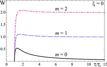
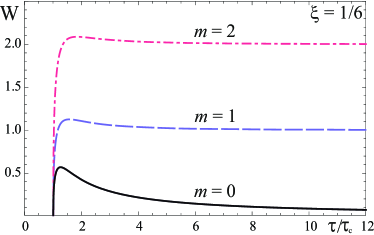
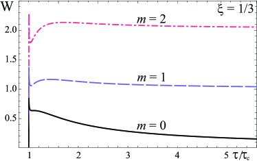
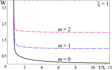
Figure 1: The solution to (50) with (23), (24), and (38), for $k=\sqrt{3/4}$, various masses, and $\xi=0$ (top left), $\xi=1/6$ (top right), $\xi=1/3$ (bottom left), and $\xi=1$ (bottom right). $W$ and $m$ are expressed in units of $\tau_{\rm c}^{-1}$.

III.3 Results

Instead of solving equation (35), for our purpose, it is convenient to solve equation (50) for the WKB function $W(\tau)$. With the help of the substitution

$$Y(\tau)=W^{-1/2}(\tau),$$ (84)

from (50) we obtain the differential equation

$$Y^{\prime\prime}+\Omega^{2}Y(\tau)-Y^{-3}=0,$$ (85)

where the function $\Omega(\tau)$ is defined in (38) with (41). Before proceeding to solve (85) for the analog cosmological model defined by the metric (20) with (23) and (24), it is useful to study three important examples which may be solved analytically.

Consider first a conformally invariant field theory, i.e., for $m=0$ and $\xi=1/6$, in which case there should be no particle creation, as has been argued on general grounds parker4 . Indeed, in this case, as may easily be verified, the function

$$Y_{\rm conf}=\omega^{-1/2}=\left(k\frac{b}{a}\right)^{-1/2}$$ (86)

is a solution to (85) for arbitrary $a(\tau)$ and $b(\tau)$. This yields $W_{\rm c}(\tau)=\omega(\tau)$ and $\omega^{(n)}=0$ at all adiabatic orders $n>0$. Then, with the choice $\tilde{W}=W^{(n)}=\omega$, by virtue of (79) we find $|\beta_{k}|=0$ and hence no particle creation as expected. In contrast, on account of (78) the choice $\tilde{W}=\Omega$ would generally yield $|\beta_{k}|\neq 0$ and hence an unphysical prediction of particle creation for a conformally invariant field.

Second, consider the asymptotic future. In the limit $\tau\rightarrow\infty$ our system approaches the zero temperature regime and the spacetime described by the analog metric (20) approaches the Milne universe with $a=\tau$ and $b=1$. It is therefore instructive to compare the analog cosmological particle creation with that of the Milne universe. In particular, in the Milne universe there should be no creation of massless particles since the scalar field satisfies the conformally invariant wave equation. Indeed, for $m=0$ the asymptotic solution to (85)

$$Y_{\infty}=\left(\frac{\tau}{k}\right)^{1/2},\quad W_{\infty}=\omega=\frac{k}{\tau},$$ (87)

gives $|\beta_{k}|^{2}=0$, and hence there is no creation of massless particles as in the previous case.

Third, it is worth analyzing the solution to (85) in the critical regime $t\equiv\tau-\tau_{\rm c}\rightarrow 0$. In that regime $\Omega^{2}\simeq\alpha t^{-2}$ where

$$\alpha=6\xi\left(\beta+\beta^{2}-\nu/4-\nu^{2}/16\right)-\beta-\beta^{2}.$$ (88)

Equation (85) then simplifies to

$$\frac{d^{2}Y}{dt^{2}}+\alpha t^{-2}Y-Y^{-3}=0$$ (89)

and may be solved analytically in the limit $t\rightarrow 0$. The behavior of the solution in that limit depends crucially on the value of the nonminimal coupling constant $\xi$. We find three distinct solutions depending on $\alpha$

$$Y=\left\{\begin{array}[]{ll}(\alpha-1/4)^{-1/4}t^{1/2},&\mbox{ for $\alpha>1/4$},\\ Y_{1}t^{1/2-\sqrt{1-4\alpha}/2},&\mbox{for $0<\alpha<1/4$},\\ Y_{2}t^{-1/2-\sqrt{1-4\alpha}/2},&\mbox{for $\alpha<0$},\end{array}\right.$$ (90)

where $Y_{1}$ and $Y_{2}$ are arbitrary real constants. Clearly, $Y\rightarrow 0$ for $\alpha>0$ and $Y\rightarrow\infty$ for $\alpha<0$. From the definition (88) it follows $\alpha\geq 0$ ($\leq 0$) if $\xi\geq\xi_{\rm c}$ ($\leq\xi_{\rm c}$) where

$$\xi_{\rm c}=\frac{1}{6}\frac{\beta+\beta^{2}}{\beta+\beta^{2}-\nu/4-\nu^{2}/16}$$ (91)

is the critical nonminimal coupling which takes the value $\xi_{\rm c}\simeq 0.28322$ for the O(4) critical exponents. Hence, the WKB function $W(\tau)$ goes to zero at the critical point if $\xi<\xi_{c}$ and diverges if $\xi>\xi_{\rm c}$. Note that the critical coupling $\xi_{\rm c}>\xi_{\rm conf}=1/6$ contrary to what one would expect since the original sigma model becomes conformally invariant at the critical point. Curiously, $\xi_{c}$ would be equal to $\xi_{\rm conf}=1/6$ if the critical exponent $\nu$ were equal to zero, in which case the pion velocity, as given by (12), would not necessarily vanish at the critical point.

Since there is no creation of pions in the limit $\tau\rightarrow\infty$, it is natural to choose as the initial state the vacuum state vector $|\;\rangle_{0}$ at some large $\tau_{0}$ and evolve equation (50) backward in time starting at $\tau_{0}$. The vacuum state satisfies

$$a_{J}|\;\rangle_{0}=0,\quad a_{J}^{\dagger}|\;\rangle_{0}=|J\rangle$$ (92)

and, according to (71), the one-particle state $|J\rangle$ is represented by

$$\langle\mbox{\boldmath{$x$}}|J\rangle=\left(\frac{1}{2\tau_{0}^{3}}\right)^{1/2}\chi_{k}^{(0)}(\tau_{0})\Phi_{J}(\mbox{\boldmath{$x$}}),$$ (93)

where the function $\chi_{k}^{(0)}(\tau)$ is defined in (55) with $W^{(0)}=\omega$. Then, the initial conditions consistent with (80) are

$$Y(\tau_{0})=\omega(\tau_{0})^{-1/2},\quad Y^{\prime}(\tau_{0})=-\frac{1}{2}\omega^{\prime}(\tau_{0})\omega(\tau_{0})^{-3/2}.$$ (94)

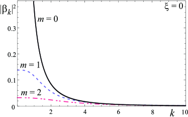
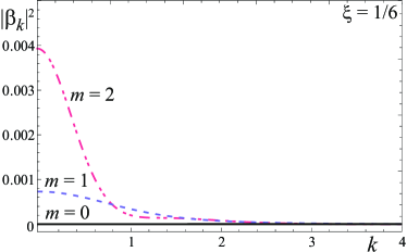
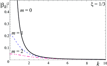
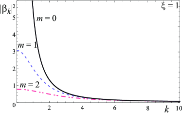
Figure 2: The square of the Bogoliubov coefficient $|\beta_{k}|^{2}$ as a function of $k$ for fixed $\tau/\tau_{\rm c}=1.12$, various masses, and $\xi=0$ (top left), $\xi=1/6$ (top right), $\xi=1/3$ (bottom left), and $\xi=1$ (bottom right).

The results of the numerical calculations are presented in Figs. 1 to 4. According to our conventions the comoving momentum $k$ is dimensionless, the time is expressed in units of $\tau_{\rm c}$, and the mass and temperature are in units of $\tau_{\rm c}^{-1}$. The proper time scale has been estimated in Sec. II.2 from the phenomenology of high energy collisions yielding a typical value $\tau_{\rm c}\approx 8.2\;{\rm fm}=41.6\;{\rm GeV}^{-1}$, so the mass scale is typically $\tau_{\rm c}^{-1}\approx 24$ MeV.

Numerical solutions to (50) with (23), (24), and (38), $W(\tau)$, are presented in Fig. 1 as functions of $\tau$ for the masses $m=0,1,2$ (in units $\tau_{\rm c}^{-1}$) and various couplings $\xi$. We use the initial conditions (94) at $\tau/\tau_{\rm c}=12$. Note a drastically different behavior of the $\xi=1/3$ and $\xi=1$ solutions (two bottom left panels) with respect to the other solutions. The reason for that is the the sign change of $\Omega^{2}$ when $\xi$ exceeds the critical value $\xi_{c}=0.28322$, as predicted by the asymptotic solution (90) in the vicinity of the critical point. Using these numerical solutions we calculate the square of the Bogoliubov coefficients $|\beta_{k}|^{2}$ as given by (79). In Fig. 2, we present $|\beta_{k}|^{2}$ as a function of $k$ for a fixed $\tau/\tau_{\rm c}=1.12$ and various couplings $\xi$.

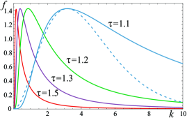
Figure 3: The spectral function $f(k)$ for $\xi=0$, and various $\tau$ expressed in units of $\tau_{\rm c}$. The dashed line represents the Planck spectral function $f_{\rm P}(k)$.

We will now use the functional form of the Planck (Bose–Einstein) particle distribution function to express

$$|\beta_{k}|^{2}=\frac{1}{e^{E/T_{\rm P}}-1},$$ (95)

where $E$ is the particle energy defined by (32) The “temperature” $T_{\rm P}$ depends on $\tau$ and is generally a function of $k$. We will call the function (95) the quasi-Planckian distribution and $T_{\rm P}$ the quasi-Planckian temperature. If $T_{\rm P}$ for a fixed $\tau$ were independent of $k$, the distribution function $|\beta_{k}|^{2}$ as a function of $k$ would have the exact Planck form (95), and the spectrum of created particles would be thermal. In this case, we would be in an exact adiabatic regime barcelo1 . If the quasi-Planckian temperature weakly depends on $k$, the spectrum will be nearly thermal. At the moment, we will assume that $T_{\rm P}$ vary weakly with $k$ and check the thermalization and adiabaticity a posteriori.

We now assume that the created pions are massless in which case $E=k/a$. To extract $T_{\rm P}$, it is convenient to use the energy density distribution function landau

$$f(k)=\frac{2\pi^{2}}{a^{3}T_{\rm P}^{3}}\frac{d\rho_{k}}{dk},$$ (96)

which we have normalized so that it depends only on the dimensionless variable $x\equiv k/(aT_{\rm P})$. For an ideal massless boson gas

$$f(k)=\frac{x^{3}}{e^{x}-1},$$ (97)

with a maximum at

$$x_{0}=2.822.$$ (98)

Using (95) we can express $f(k)$ as

$$f(k)=|\beta_{k}|^{2}\ln(1+1/|\beta_{k}|^{2})^{3}$$ (99)

and plot the right-hand side as a function of $k$ for various $\tau$ (Fig. 3). Then, from the position of the maximum $k_{\rm max}(\tau)$ we obtain

$$T_{\rm P}(\tau)=\frac{k_{\rm max}(\tau)}{x_{0}a(\tau)}.$$ (100)

For the purpose of comparison, in Fig. 3, we also plot the exact Planck spectral function $f_{\rm P}(k)$ given by (97) with a $k$-independent temperature $T_{\rm P}$. The temperature $T_{\rm P}$ is determined from (100) so that $f_{\rm P}(k)$ coincides with our spectral function $f(k)$ at $k=k_{\rm max}$ corresponding to $\tau=1.1$. A comparison between $f(k)$ and $f_{\rm P}(k)$ (Fig. 3) shows that our quasi-Planckian spectrum is close to the Planckian for the wave numbers near $k_{\rm max}$ and left from $k_{\rm max}$. Clearly, the departure of $f(k)$ from $f_{\rm P}(k)$ is significant for large $k$ because, according to (83), $f(k)$ falls off asymptotically as $k^{-4}(\ln{k})^{3}$ in contrast to the exponential decay of $f_{\rm P}(k)$. Hence, the calculated quasi-Planckian temperature $T_{\rm P}$ may be regarded as reliable for almost all particles with wave numbers $k\lesssim k_{\rm max}$ and some particles with $k$ above $k_{\rm max}$. The number of particles thermalized at $T_{\rm P}$ may be estimated by performing the integral in (77) with the exact Planck distribution function given by (95) with a $k$-independent temperature $T_{\rm P}$. The excess of unthermalized particles above $k_{\rm max}$ may be estimated evaluating the integral from $k_{\rm max}$ to $\infty$ using the same Planck distribution subtracted from the asymptotic expression (83). We find that the proportion of such particles to the total number of thermalized ones amounts to less than $20\%$ at $\tau=1.1$ and less than $25\%$ at $\tau=1.05$.

To check how close we are to the adiabatic regime, for each $\tau$ we compare the comoving wave number $k$ with the Hubble scale $|H|$. As usual, we distinguish three regimes: the adiabatic regime in which $k\gg|H|$, the sudden regime in which $k\ll|H|$, and the intermediate regime in which $k\approx|H|$ barcelo1 . For large $\tau$ we have $H\simeq 1/\tau$ and we are clearly in the adiabatic regime for almost all wave numbers since the criteria $k\gg 1/\tau$ is easily met. However, we expect a departure from adiabaticity in the limit $\tau\rightarrow\tau_{\rm c}$ since in this limit $H$ diverges according to (26). For example, for $\tau=1.1$ we find $|H|\simeq 3$, so the wave numbers satisfying $k\lesssim 3$ are not in the adiabatic regime. In the region of $\tau$ between 1.5 and 1.1 depicted in Fig. 3, using (26) we find $0.3\lesssim|H|\lesssim 3$ corresponding to $0.4\lesssim k_{\rm max}\lesssim 3$, so our estimated $k_{\rm max}$ are of the order of $|H|$ and fall into the intermediate regime.

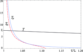
Figure 4: The quasi-Planckian temperature $T_{\rm P}$ as a function of $\tau$ for $\xi=0$ compared with the Hawking temperature $T_{\rm H}$ and the temperature of the fluid $T=T_{\rm c}\tau_{\rm c}/\tau$. The temperatures are plotted in units of $\tau_{\rm c}^{-1}$. The label $T_{\rm c}$ at 7.625 on the vertical axis marks the critical temperature.

In Fig. 4, we plot the quasi-Planckian temperature as a function of $\tau$ for vanishing nonminimal coupling constant $\xi$ together with the Hawking temperature $T_{\rm H}$ of thermal pions emitted at the apparent horizon. For comparison we plot in the same figure the background temperature of the fluid vs $\tau$ as given by equation (22) with $T_{\rm c}=$ 7.625 $\tau_{\rm c}^{-1}$.

The functional dependence of $T_{\rm H}$ is calculated following the prescription of our previous papers tolic ; tolic2 . As shown in Ref.  tolic2 , the condition that a two-dimensional surface $H$ is the apparent horizon for a spherically symmetric spacetime may be expressed as

$$G^{\mu\nu}n_{\mu}n_{\nu}|_{H}=0,$$ (101)

where $n_{\mu}$ is a vector field normal to the surfaces of spherical symmetry. For the metric (20) the vector $n_{\mu}$ is given by

$$n_{\mu}=\partial_{\mu}(a\sinh y).$$ (102)

Using this and (101) we obtain the condition for the analog apparent horizon in the form

$$\frac{\dot{a}}{b}\pm\frac{1}{\tanh y}=0.$$ (103)

Provided this condition is met, the surface gravity $\kappa$ at the horizon may be calculated using the Kodama–Hayward prescription hayward2 which we have adapted to analog gravity tolic . This prescription involves theso-called Kodama vector $K^{\mu}$ kodama which generalizes the concept of the time translation Killing vector to nonstationary spacetimes. The analog surface gravity $\kappa$ is defined by

$$\kappa=\frac{1}{2}\frac{1}{\sqrt{-h}}\partial_{\alpha}(\sqrt{-h}h^{\alpha\beta}Kn_{\beta}),$$ (104)

where the quantities on the right-hand side should be evaluated at the apparent horizon. The tensor $h^{\alpha\beta}$ is the inverse of the metric $h_{\alpha\beta}$ of the two-dimensional space normal to the surface of spherical symmetry and $h=\det h_{\alpha\beta}$. The definition (104) differs from the original expression for the dynamical surface gravity hayward2 by a normalization factor $K$ which we have introduced in order to meet the requirement that $K^{\mu}$ should coincide with the time translation Killing vector $\xi^{\mu}$ for a stationary geometry. The details of the calculation and the final expression for $\kappa$ may be found in Ref. tolic . The corresponding temperature $T_{\rm H}=\kappa/(2\pi)$ represents the analog Hawking temperature of thermal pions emitted at the apparent horizon.

As shown in Ref. tolic , the Hawking temperature diverges near the critical point as

$$T_{\rm H}\propto(\tau-\tau_{\rm c})^{-1}.$$ (105)

The temperature $T_{\rm P}$ seems to diverge at the critical point in a similar way and vanishes in the limit $\tau\rightarrow\infty$ corresponding to the zero background temperature of the hadronic fluid. In contrast, the analog Hawking temperature vanishes at $\tau=\tau_{\rm max}=$ 1.1002 $\tau_{\rm c}$ at which the analog trapping horizon ceases to exist tolic2 .

IV Conclusions

We have investigated the cosmological creation of pions in an expanding hadronic fluid in the regime near the critical point of the chiral phase transition. In our approach we have disregarded a possible particle production caused by the self-interaction potential of the scalar field. Besides, we have assumed that the created pions are of zero or very light mass and we have neglected the creation of much heavier sigma mesons. The production rate has been calculated using the adiabatic regularization prescription according to which the Bogoliubov coefficients are expressed in terms of the WKB function $W(\tau)$ and its first-order adiabatic approximation $W^{(1)}(\tau)=\omega(\tau)$. The function $W(\tau)$ has been computed by solving equation (50) numerically. We have analyzed more closely the solution in the limit when $\tau$ approaches the critical value. It turns out that the behavior of the solution in that limit depends crucially on the value of the nonminimal coupling constant $\xi$. We have shown that there exists a certain critical value $\xi_{\rm c}$ larger than the conformal value $\xi=1/6$ such that $W(\tau)$ goes to zero at the critical point for $\xi<\xi_{\rm c}$ and diverges for $\xi>\xi_{\rm c}$.

We have calculated the cosmological production rate as a function of the proper time for various masses and various nonminimal coupling constants $\xi$. The production rate of massless pions shows a strong dependence on $\xi$ and vanishes for $\xi=1/6$ as it should. By fitting the production rate to the Planck blackbody radiation spectrum we have extracted the temperature of the produced pion gas. We use the time dependence of the thus obtained quasi-Planckian temperature to compare the analog Hawking effect with the analog cosmological particle creation. As we have already mentioned, these two effects, although being of similar quantum origin, are quite distinct physical phenomena that appear under different physical conditions. Compared with the analog Hawking radiation of pions at the trapping horizon, the spectrum of the cosmological radiation shows a similar behavior near the critical point. The temperature of the cosmologically created pions $T_{\rm P}$ diverges at the critical point roughly in the same way as the analog Hawking temperature $T_{\rm H}$. However, as the proper time increases, the quasi-Planckian temperature vanishes asymptotically whereas the analog Hawking temperature vanishes at a finite proper time of the order 1.1 $\tau_{\rm c}$ when the analog trapping horizon disappears.

Our results could not be easily confronted with observations. First of all, we are dealing with exact spherical symmetry, whereas in most high energy collisions the symmetry is axial involving a transverse expansion superimposed on a longitudinal boost invariant expansion. Second, the cosmologically created and Hawking radiated pions could not be easily distinguished from the background pions produced directly from the quark-gluon plasma (QGP). Nevertheless, we can draw a qualitative postcollision picture as follows.

The high temperature (QGP) produced in the collision expands and cools down until the temperature is as low as the deconfinement temperature of the order of $T_{\rm dec}\simeq T_{\rm c}=183$. Then, a hadronic fluid mainly consisting of pions forms and expands further according to the Bjorken model with the proper time related to the background fluid temperature through the relation (22), where $\tau_{\rm c}^{-1}\simeq 24$ MeV. Immediately below $T_{\rm c}=183$, the cosmological creation and the Hawking radiation take place. Initially, both the Hawking and quasi-Planckian temperatures exceed the background fluid temperature $T$ by a factor of $2$ or more. As a consequence, a considerable fraction of the pion gas will be briefly “reheated” but, according to Fig. 1, will quickly cool down during the subsequent expansion. Whereas the Hawking radiation stops at $\tau=\tau_{\max}$ when the temperature of the fluid is of the order 0.9 $T_{\rm c}$, the cosmological creation continues up to the thermal freez-out. The thermal (or kinetic) freezout takes place soon after the so-called chemical freez-out which is very close or equal to the QCD deconfinement transition braun . The kinetic freez-out temperature depends on the collision energy star and is roughly between 0.7 and 0.9 $T_{\rm c}$, which corresponds to the proper time interval $(1.1,1.4)$. From Fig. 4 it is evident that the influence of the cosmological production and the Hawking radiation will be more pronounced if the thermal freez-out is closer to the critical temperature.

Acknowledgments

We gratefully acknowledge enlightening discussions with S. Liberati and M. Visser which motivated us to consider particle creation in the hadronic analog universe. This work has been supported by the Croatian Science Foundation under the project (IP-2014-09-9582) and supported in part by the ICTP-SEENET-MTP Grant No. PRJ-09 “Strings and Cosmology” in the frame of the SEENET-MTP Network.

References

- (1) L. Parker, Ph.D. thesis, Harvard University, 1966; Phys. Rev. Lett. 21, 562 (1968); Phys. Rev. 183, 1057 (1969).
- (2) T. Jacobson, arXiv:gr-qc/0308048.
- (3) C. Barcelo, S. Liberati, and M. Visser, Phys. Rev. A 68, 053613 (2003) [arXiv:cond-mat/0307491].
- (4) P. Jain, S. Weinfurtner, M. Visser, and C. W. Gardiner, Phys. Rev. A 76, 033616 (2007) [arXiv:0705.2077]; Class. Quant. Grav. 26, 065012 (2009) [arXiv:0801.2673 [gr-qc]].
- (5) Y. Kurita, M. Kobayashi, H. Ishihara, M. Tsubota, Phys. Rev. A 82, 053602 (2010) [arXiv:1007.0073].
- (6) C. Sabìn and I. Fuentes, arXiv:1405.5789 [quant-ph].
- (7) P. O. Fedichev and U. R. Fischer, Phys. Rev. A 69, 033602 (2004) [cond-mat/0303063].
- (8) N. Bilić and D. Tolić, Phys. Lett. B 718, 223 (2012) [arXiv:1207.2869 [hep-th]].
- (9) N. Bilić and D. Tolić, Phys. Rev. D 87, 044033 (2013) [arXiv:1210.3824 [gr-qc]].
- (10) C. Barcelo, S. Liberati, and M. Visser, Living Rev. Rel. 8, 12 (2005) [gr-qc/0505065].
- (11) M. Visser, Class. Quant. Grav. 15, 1767 (1998) [arXiv:gr-qc/9712010].
- (12) T. G. Philbin, C. Kuklewicz, S. Robertson, S. Hill, F. Konig, and U. Leonhardt, Science 319, 1367 (2008) [arXiv:0711.4796 [gr-qc]].
- (13) T.A. Jacobson and G.E. Volovik, Phys. Rev. D 58, 064021 (1998) [arXiv:cond-mat/9801308].
- (14) V. Moncrief, Astrophys. J. 235, 1038 (1980).
- (15) H. Abraham, N. Bilić and T. K. Das, Class. Quant. Grav. 23, 2371 (2006) [gr-qc/0509057]. T. K. Das, N. Bilić and S. Dasgupta, JCAP 0706, 009 (2007) [astro-ph/0604477]; N. Bilić, A. Choudhary, T. K. Das and S. Nag, Class. Quant. Grav. 31, 035002 (2014) [arXiv:1205.5506 [gr-qc]].
- (16) N. Bilic and D. Tolic, Phys. Rev. D 88, 105002 (2013) [arXiv:1309.2833 [gr-qc]].
- (17) M.A. Shifman, Ann. Rev. Nucl. Part. Sci. 33, 199 (1983).
- (18) J. W. Harris and B. Müller, Ann. Rev. Nucl. Part. Sci. 46, 71 (1996).
- (19) M. Gell-Mann and M. Lévy, Nuovo Cimento 16, 705 (1960).
- (20) M. A. Lampert, J. F. Dawson and F. Cooper, Phys. Rev. D 54, 2213 (1996) [hep-th/9603068]; G. Amelino-Camelia, J. D. Bjorken and S. E. Larsson, Phys. Rev. D 56, 6942 (1997) [hep-ph/9706530]; M. A. Lampert and C. Molina-Paris, Phys. Rev. D 57, 83 (1998) [hep-ph/9708380]; A. Krzywicki and J. Serreau, Phys. Lett. B 448, 257 (1999) [hep-ph/9811346].
- (21) N. Bilic, J. Cleymans and M. D. Scadron, Int. J. Mod. Phys. A 10, 1169 (1995) [hep-ph/9402201].
- (22) N. Bilic and H. Nikolic, Eur. Phys. J. C 6, 515 (1999) [hep-ph/9711513].
- (23) R. D. Pisarski and M. Tytgat, Phys. Rev. D 54, R2989 (1996) [hep-ph/9604404].
- (24) D. T. Son and M. A. Stephanov, Phys. Rev. Lett. 88, 202302 (2002) [hep-ph/0111100].
- (25) D. T. Son and M. A. Stephanov, Phys. Rev. D 66, 076011 (2002) [hep-ph/0204226].
- (26) A.A. Grib, S.G. Mamayev, and V.M. Mostepanenko, Vacuum Quantum Effects in Strong Fields, (Energoatomizdat, Moscow, 1988 (in Russian) and Friedmann Lab. Publishing, St. Petersburg, 1994 (English translation))
- (27) L.E. Parker and D.J. Toms, Quantum Field Theory in Curved Spacetime, (Cambridge University Press, Cambridge, 2009)
- (28) A. J. Hamilton, D. N. Kabat and M. K. Parikh, JHEP 0407, 024 (2004) [hep-th/0311180].
- (29) E. Greenwood, arXiv:1402.4557 [gr-qc].
- (30) N. Bilić and H. Nikolić, Phys. Rev. D 68, 085008 (2003) [hep-ph/0301275].
- (31) M. Hasenbusch, J. Phys. A 34 (2001) 8221 [cond-mat/0010463].
- (32) F. Parisen Toldin, A. Pelissetto and E. Vicari, JHEP 0307, 029 (2003) [hep-ph/0305264].
- (33) N. Bilic, Class. Quant. Grav. 16, 3953 (1999) [gr-qc/9908002].
- (34) M. Visser and C. Molina-Paris, New J. Phys. 12, 095014 (2010) [arXiv:1001.1310 [gr-qc]].
- (35) J. D. Bjorken, Phys. Rev. D 27, 140 (1983).
- (36) S. Fagnocchi, S. Finazzi, S. Liberati, M. Kormos, and A. Trombettoni, New J. Phys. 12, 095012 (2010). [arXiv:1001.1044 [gr-qc]].
- (37) E.A. Milne, Nature 130 (1932) 9.
- (38) L.D. Landau and E.M. Lifshitz, Statistical Physics, (Pergamon, Oxford, 1993) p. 187.
- (39) P. F. Kolb, J. Sollfrank, and U. W. Heinz, Phys. Rev. C 62, 054909 (2000) [hep-ph/0006129]; V. N. Russkikh and Y. .B. Ivanov, Phys. Rev. C 76, 054907 (2007) [nucl-th/0611094].
- (40) N.D. Birrell, P.C.W. Davies, Quantum Fields in Curved Space, Cambridge University Press, Cambridge, 1992.
- (41) L.E. Parker and D.J. Toms, Phys. Rev. D 31, 2424 (1985)
- (42) L. Parker, J. Phys. A 45, 374023 (2012) [arXiv:1205.5616 [astro-ph.CO]].
- (43) S.A. Fulling, Gen. Rel. Grav. 10, 807 (1979).
- (44) A. Landete, J. Navarro-Salas and F. Torrenti, Phys. Rev. D 89, 044030 (2014) [arXiv:1311.4958 [gr-qc]].
- (45) Yu. V. Pavlov, Grav. Cosmol. 14, 314 (2008) [arXiv:0811.4236 [gr-qc]].
- (46) S. A. Hayward, Class. Quant. Grav. 15, 3147 (1998).
- (47) H. Kodama, Prog. Theor. Phys. 63, 1217 (1980).
- (48) P. Braun-Munzinger, J. Stachel and C. Wetterich, Phys. Lett. B 596, 61 (2004) [nucl-th/0311005]; A. Bazavov et al., Phys. Rev. Lett. 109, 192302 (2012) [arXiv:1208.1220 [hep-lat]]; F. Becattini, E. Grossi, M. Bleicher, J. Steinheimer and R. Stock, Phys. Rev. C 90, 054907 (2014) [arXiv:1405.0710 [nucl-th]].
- (49) B. I. Abelev et al. [STAR Collaboration], Phys. Rev. C 79, 034909 (2009); [arXiv:0808.2041 [nucl-ex]]. M. M. Aggarwal et al. [STAR Collaboration], Phys. Rev. C 83, 034910 (2011) [arXiv:1008.3133 [nucl-ex]]; L. Kumar [STAR Collaboration], J. Phys. G 38, 124145 (2011) [arXiv:1106.6071 [nucl-ex]].