Reconfiguration of Cliques in a Graph

Abstract

We study reconfiguration problems for cliques in a graph, which determine whether there exists a sequence of cliques that transforms a given clique into another one in a step-by-step fashion. As one step of a transformation, we consider three different types of rules, which are defined and studied in reconfiguration problems for independent sets. We first prove that all the three rules are equivalent in cliques. We then show that the problems are PSPACE-complete for perfect graphs, while we give polynomial-time algorithms for several classes of graphs, such as even-hole-free graphs and cographs. In particular, the shortest variant, which computes the shortest length of a desired sequence, can be solved in polynomial time for chordal graphs, bipartite graphs, planar graphs, and bounded treewidth graphs.

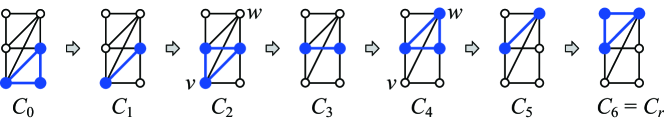
Figure 1: A sequence $\langle C_{0},C_{1},\ldots,C_{6}\rangle$ of cliques in the same graph, where the vertices in cliques are depicted by large (blue) circles (tokens).

1 Introduction

Recently, reconfiguration problems attract attention in the field of theoretical computer science. The problem arises when we wish to find a step-by-step transformation between two feasible solutions of a problem such that all intermediate results are also feasible and each step abides by a fixed reconfiguration rule (i.e., an adjacency relation defined on feasible solutions of the original problem). This kind of reconfiguration problem has been studied extensively for several well-known problems, including satisfiability [10], independent set [3, 11, 12, 14, 22], vertex cover [13, 16], clique, matching [12], vertex-coloring [2], and so on. (See also a recent survey [21].)

It is well known that independent sets, vertex covers and cliques are related with each other. Indeed, the well-known reductions for NP-completeness proofs are essentially the same for the three problems [7]. Despite reconfiguration problems for independent sets and vertex covers are two of the most well studied problems, we have only a few known results for reconfiguration problems for cliques (as we will explain later). In this paper, we thus investigate the complexity status of reconfiguration problems for cliques systematically, and show that the problems can be solved in polynomial time for a variety of graph classes, in contrast to independent sets and vertex covers.

1.1 Our problems and three rules

Recall that a clique of a graph $G=(V,E)$ is a vertex subset of $G$ in which every two vertices are adjacent. (Figure 1 depicts seven different cliques in the same graph.) Suppose that we are given two cliques $C_{0}$ and $C_{r}$ of $G$, and imagine that a token is placed on each vertex in $C_{0}$. Then, we are asked to transform $C_{0}$ into $C_{r}$ by abiding a prescribed reconfiguration rule on cliques. In this paper, we define three different reconfiguration rules on cliques, which were originally defined as the reconfiguration rules on independents sets [14], as follows:

• Token Addition and Removal ($\mathsf{TAR}$ rule): We can either add or remove a single token at a time if it results in a clique of size at least a given threshold $k\geq 0$. For example, in the sequence $\langle C_{0},C_{1},\ldots,C_{6}\rangle$ in Figure 1, every two consecutive cliques follow the $\mathsf{TAR}$ rule for the threshold $k=2$. In order to emphasize the threshold $k$, we sometimes call this rule the $\mathsf{TAR}(k)$ rule.

• Token Jumping ($\mathsf{TJ}$ rule): A single token in a clique $C$ can “jump” to any vertex in $V\setminus C$ if it results in a clique. For example, consider the sequence $\langle C_{0},C_{2},C_{4},C_{6}\rangle$ in Figure 1, then two consecutive cliques $C_{2i}$ and $C_{2i+2}$ follow the $\mathsf{TJ}$ rule for each $i\in\{0,1,2\}$.

• Token Sliding ($\mathsf{TS}$ rule): We can slide a single token on a vertex $v$ in a clique $C$ to another vertex $w$ in $V\setminus C$ if it results in a clique and there is an edge $vw$ in $G$. For example, consider the sequence $\langle C_{2},C_{4}\rangle$ in Figure 1, then two consecutive cliques $C_{2}$ and $C_{4}$ follow the $\mathsf{TS}$ rule, because $v$ and $w$ are adjacent.

A sequence $\langle C_{0},C_{1},\ldots,C_{\ell}\rangle$ of cliques of a graph $G$ is called a reconfiguration sequence between two cliques $C_{0}$ and $C_{\ell}$ under $\mathsf{TAR}(k)$ (or $\mathsf{TJ}$, $\mathsf{TS}$) if two consecutive cliques $C_{i-1}$ and $C_{i}$ follow the $\mathsf{TAR}(k)$ (resp., $\mathsf{TJ}$, $\mathsf{TS}$) rule for all $i\in\{1,2,\ldots,\ell\}$. The length of a reconfiguration sequence is defined to be the number of cliques in the sequence minus one, that is, the length of $\langle C_{0},C_{1},\ldots,C_{\ell}\rangle$ is $\ell$.

Given two cliques $C_{0}$ and $C_{r}$ of a graph $G$ (and an integer $k\geq 0$ for $\mathsf{TAR}$), clique reconfiguration under $\mathsf{TAR}$ (or $\mathsf{TJ}$, $\mathsf{TS}$) is to determine whether there exists a reconfiguration sequence between $C_{0}$ and $C_{r}$ under $\mathsf{TAR}(k)$ (resp., $\mathsf{TJ}$, $\mathsf{TS}$). For example, consider the cliques $C_{0}$ and $C_{r}=C_{6}$ in Figure 1; let $k=2$ for $\mathsf{TAR}$. Then, it is a $\mathsf{yes}$-instance under the $\mathsf{TAR}(2)$ and $\mathsf{TJ}$ rules as illustrated in Figure 1, but is a $\mathsf{no}$-instance under the $\mathsf{TS}$ rule.

In this paper, we also study the shortest variant, called shortest clique reconfiguration, under each of the three rules which computes the shortest length of a reconfiguration sequence between two given cliques under the rule. We define the shortest length to be infinity for a $\mathsf{no}$-instance, and hence this variant is a generalization of clique reconfiguration.

1.2 Known and related results

Ito et al. [12] introduced clique reconfiguration under $\mathsf{TAR}$, and proved that it is PSPACE-complete in general. They also considered the optimization problem of computing the maximum threshold $k$ such that there is a reconfiguration sequence between two given cliques $C_{0}$ and $C_{r}$ under $\mathsf{TAR}(k)$. This maximization problem cannot be approximated in polynomial time within any constant factor unless ${\rm P}={\rm NP}$ [12].

Independent set reconfiguration is one of the most well-studied reconfiguration problems, defined for independent sets in a graph. Kamiński et al. [14] studied the problem under $\mathsf{TAR}$, $\mathsf{TJ}$ and $\mathsf{TS}$. It is well known that a clique in a graph $G$ forms an independent set in the complement $\overline{G}$ of $G$, and vice versa. Indeed, some known results for independent set reconfiguration can be converted into ones for clique reconfiguration. However, as far as we checked, only two results can be obtained for clique reconfiguration by this conversion, because we take the complement of a graph. (These results will be formally discussed in Section 3.3.)

In this way, only a few results are known for clique reconfiguration. In particular, there is almost no algorithmic result, and hence it is desired to develop efficient algorithms for the problem and its shortest variant.

1.3 Our contribution

In this paper, we embark on a systematic investigation of the computational status of clique reconfiguration and its shortest variant. Figure 2 summarizes our results, which can be divided into the following four parts.

• Rule equivalence (Section 3): We prove that all rules $\mathsf{TAR}$, $\mathsf{TS}$ and $\mathsf{TJ}$ are equivalent in clique reconfiguration. Then, any complexity result under one rule can be converted into the same complexity result under the other two rules. In addition, based on the rule equivalence, we show that clique reconfiguration under any rule is PSPACE-complete for perfect graphs, and is solvable in linear time for cographs.

• Graphs with bounded clique size (Section 4.1): We show that the shortest variant under any of $\mathsf{TAR}$, $\mathsf{TS}$ and $\mathsf{TJ}$ can be solved in polynomial time for such graphs, which include bipartite graphs, planar graphs, and bounded treewidth graphs. Interestingly, independent set reconfiguration under any rule remains PSPACE-complete even for planar graphs [2, 11] and bounded treewidth graphs [22]. Therefore, this result shows a nice difference between the reconfiguration problems for cliques and independent sets.

• Graphs with polynomially many maximal cliques (Section 4.2): We show that clique reconfiguration under any of $\mathsf{TAR}$, $\mathsf{TS}$ and $\mathsf{TJ}$ can be solved in polynomial time for such graphs, which include even-hole-free graphs, graphs of bounded boxicity, and $K_{t}$-subdivision-free graphs.

• Chordal graphs (Section 5): We give a linear-time algorithm to solve the shortest variant under any of $\mathsf{TAR}$, $\mathsf{TS}$ and $\mathsf{TJ}$ for chordal graphs. Note that the clique size of chordal graphs is not always bounded, and hence this result is independent from Result (2) above.

Several proofs move to appendices.

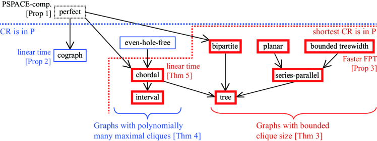
Figure 2: Our results under all rules $\mathsf{TAR}$, $\mathsf{TS}$ and $\mathsf{TJ}$. Each arrow represents the inclusion relationship between graph classes: $A\to B$ represents that $B$ is properly included in $A$ [4]. Graph classes for which shortest clique reconfiguration is solvable in polynomial time are indicated by thick (red) boxes, while the ones for which clique reconfiguration is solvable in polynomial time are indicated by thin (blue) boxes.

2 Preliminaries

In this section, we introduce some basic terms and notation.

2.1 Graph notation

In this paper, we assume without loss of generality that graphs are simple. For a graph $G$, we sometimes denote by $V(G)$ and $E(G)$ the vertex set and edge set of $G$, respectively. For a graph $G$, the complement $\overline{G}$ of $G$ is the graph such that $V(\overline{G})=V(G)$ and $E(\overline{G})=\{vw\mid v,w\in V(G),\ vw\not\in E(G)\}$. We say that a graph class $\mathcal{G}$ (i.e., a set of graphs) is closed under taking complements if $\overline{G}\in\mathcal{G}$ holds for every graph $G\in\mathcal{G}$.

In this paper, we deal with several graph classes systematically, and hence we do not define those graph classes precisely; we simply give the properties used for proving our results, with appropriate references.

2.2 Definitions for clique reconfiguration

As explained in Introduction, we consider three (symmetric) adjacency relations on cliques in a graph. Let $C_{i}$ and $C_{j}$ be two cliques of a graph $G$. Then,

• $C_{i}\leftrightarrow C_{j}$ under $\mathsf{TAR}(k)$ for a nonnegative integer $k$ if $|C_{i}|\geq k$, $|C_{j}|\geq k$, and $|C_{i}\vartriangle C_{j}|=\bigl{|}(C_{i}\setminus C_{j})\cup(C_{j}\setminus C_{i})\bigr{|}=1$ hold;

• $C_{i}\leftrightarrow C_{j}$ under $\mathsf{TJ}$ if $|C_{i}|=|C_{j}|$, $|C_{i}\setminus C_{j}|=1$, and $|C_{j}\setminus C_{i}|=1$ hold; and

• $C_{i}\leftrightarrow C_{j}$ under $\mathsf{TS}$ if $|C_{i}|=|C_{j}|$, $C_{i}\setminus C_{j}=\{v\}$, $C_{j}\setminus C_{i}=\{w\}$, and $vw\in E(G)$ hold.

A sequence $\langle C_{1},C_{2},\ldots,C_{\ell}\rangle$ of cliques of $G$ is called a reconfiguration sequence between two cliques $C_{1}$ and $C_{\ell}$ under $\mathsf{TAR}(k)$ (or $\mathsf{TJ}$, $\mathsf{TS}$) if $C_{i-1}\leftrightarrow C_{i}$ holds under $\mathsf{TAR}(k)$ (resp., $\mathsf{TJ}$, $\mathsf{TS}$) for all $i\in\{2,3,\ldots,\ell\}$. A reconfiguration sequence under $\mathsf{TAR}(k)$ (or $\mathsf{TJ}$, $\mathsf{TS}$) is simply called a $\mathsf{TAR}(k)$-sequence (resp., $\mathsf{TJ}$-sequence, $\mathsf{TS}$-sequence). We write $C_{1}\leftrightsquigarrow C_{\ell}$ under $\mathsf{TAR}(k)$ (or $\mathsf{TJ}$, $\mathsf{TS}$) if there exists a $\mathsf{TAR}(k)$-sequence (resp., $\mathsf{TJ}$-sequence, $\mathsf{TS}$-sequence) between $C_{1}$ and $C_{\ell}$. Note that each clique in any $\mathsf{TAR}(k)$-sequence is of size at least $k$, while all cliques in any $\mathsf{TJ}$-sequence or $\mathsf{TS}$-sequence have the same size. In addition, a reconfiguration sequence under any rule is reversible, that is, $C_{1}\leftrightsquigarrow C_{\ell}$ if and only if $C_{\ell}\leftrightsquigarrow C_{1}$.

Let $k$ be a nonnegative integer, and let $C$ and $C^{\prime}$ be two cliques of a graph $G$. Then, we define $\mathsf{TAR}(C,C^{\prime},k)$, as follows:

$$\mathsf{TAR}(C,C^{\prime},k)=\left\{\begin{array}[]{ll}\mathsf{yes}&~{}~{}~{}\mbox{if $C\leftrightsquigarrow C^{\prime}$ under $\mathsf{TAR}(k)$};\\ \mathsf{no}&~{}~{}~{}\mbox{otherwise}.\end{array}\right.$$

Given two cliques $C_{0}$ and $C_{r}$ of a graph $G$ and a nonnegative integer $k$, clique reconfiguration under $\mathsf{TAR}$ is to compute $\mathsf{TAR}(C_{0},C_{r},k)$. By the definition, $\mathsf{TAR}(C_{0},C_{r},k)=\mathsf{no}$ if $|C_{0}|<k$ or $|C_{r}|<k$ hold, and hence we may assume without loss of generality that both $|C_{0}|\geq k$ and $|C_{r}|\geq k$ hold; we call such an instance simply a $\mathsf{TAR}$-instance, and denote it by $(G,C_{0},C_{r},k)$.

For two cliques $C$ and $C^{\prime}$ of a graph $G$, we similarly define $\mathsf{TJ}(C,C^{\prime})$ and $\mathsf{TS}(C,C^{\prime})$. Given two cliques $C_{0}$ and $C_{r}$ of $G$, we similarly define clique reconfiguration under $\mathsf{TJ}$ and $\mathsf{TS}$, and denote their instance by $(G,C_{0},C_{r})$. Then, we can assume that $|C_{0}|=|C_{r}|$ holds in a $\mathsf{TJ}$- or a $\mathsf{TS}$-instance $(G,C_{0},C_{r})$.

Given a $\mathsf{TAR}$-instance $(G,C_{0},C_{r},k)$, let $\mathcal{C}=\langle C_{0},C_{1},\ldots,C_{\ell}\rangle$ be a $\mathsf{TAR}(k)$-sequence in $G$ between $C_{0}$ and $C_{r}=C_{\ell}$. Then, the length of $\mathcal{C}$ is defined to be the number of cliques in $\mathcal{C}$ minus one, that is, the length of $\mathcal{C}$ is $\ell$. We denote by $\mathsf{dist_{TAR}}(G,C_{0},C_{r},k)$ the minimum length of a $\mathsf{TAR}(k)$-sequence in $G$ between $C_{0}$ and $C_{r}$; we let $\mathsf{dist_{TAR}}(G,C_{0},C_{r},k)=+\infty$ if there is no $\mathsf{TAR}(k)$-sequence in $G$ between $C_{0}$ and $C_{r}$. The shortest variant, shortest clique reconfiguration, under $\mathsf{TAR}$ is to compute $\mathsf{dist_{TAR}}(G,C_{0},C_{r},k)$. Similarly, we define $\mathsf{dist_{TJ}}(G,C_{0},C_{r})$ and $\mathsf{dist_{TS}}(G,C_{0},C_{r})$ for a $\mathsf{TJ}$- and a $\mathsf{TS}$-instance $(G,C_{0},C_{r})$, respectively. Then, shortest clique reconfiguration under $\mathsf{TJ}$ or $\mathsf{TS}$ is defined similarly. We sometimes drop $G$ and simply write $\mathsf{dist_{TAR}}(C_{0},C_{r},k)$, $\mathsf{dist_{TJ}}(C_{0},C_{r})$ and $\mathsf{dist_{TS}}(C_{0},C_{r})$ if it is clear from context.

We note that clique reconfiguration under any rule is a decision problem asking for the existence of a reconfiguration sequence, and its shortest variant asks for simply computing the shortest length of a reconfiguration sequence. Therefore, the problems do not ask for an actual reconfiguration sequence. However, our algorithms proposed in this paper can be easily modified so that they indeed find a reconfiguration sequence.

3 Rule Equivalence and Complexity

In this section, we first prove that all three rules $\mathsf{TAR}$, $\mathsf{TS}$ and $\mathsf{TJ}$ are equivalent in clique reconfiguration. We then discuss some complexity results that can be obtained from known results for independent set reconfiguration.

3.1 Equivalence of $\mathsf{TS}$ and $\mathsf{TAR}$ rules

$\mathsf{TS}$ and $\mathsf{TAR}$ rules are equivalent, as in the following sense.

Theorem 3.1

$\mathsf{TS}$ and $\mathsf{TAR}$ rules are equivalent in clique reconfiguration, as follows:

• for any $\mathsf{TS}$-instance $(G,C_{0},C_{r})$, a $\mathsf{TAR}$-instance $(G,C_{0}^{\prime},C_{r}^{\prime},k^{\prime})$ can be constructed in linear time such that $\mathsf{TS}(C_{0},C_{r})=\mathsf{TAR}(C_{0}^{\prime},C_{r}^{\prime},k^{\prime})$ and $\mathsf{dist_{TS}}(C_{0},C_{r})=\mathsf{dist_{TAR}}(C_{0}^{\prime},C_{r}^{\prime},k^{\prime})/2$; and

• for any $\mathsf{TAR}$-instance $(G,C_{0},C_{r},k)$, a $\mathsf{TS}$-instance $(G,C_{0}^{\prime},C_{r}^{\prime})$ can be constructed in linear time such that $\mathsf{TAR}(C_{0},C_{r},k)=\mathsf{TS}(C_{0}^{\prime},C_{r}^{\prime})$.

By Theorem 3.1(a), note that the reduction from $\mathsf{TS}$ to $\mathsf{TAR}$ preserves the shortest length of reconfiguration sequences.

Proof of Theorem 3.1(a). Let $(G,C_{0},C_{r})$ be a $\mathsf{TS}$-instance with $|C_{0}|=|C_{r}|=k$. Then, as the corresponding $\mathsf{TAR}$-instance $(G,C_{0}^{\prime},C_{r}^{\prime},k^{\prime})$, we let $C_{0}^{\prime}=C_{0}$, $C_{r}^{\prime}=C_{r}$ and $k^{\prime}=k$; this $\mathsf{TAR}$-instance can be clearly constructed in linear time. We thus prove the following lemma, as a proof of Theorem 3.1(a).

Lemma 1

Let $G$ be a graph, and let $C_{0}$ and $C_{r}$ be any pair of cliques of $G$ such that $|C_{0}|=|C_{r}|=k$. Then, $\mathsf{TS}(C_{0},C_{r})=\mathsf{TAR}(C_{0},C_{r},k)$ and $\mathsf{dist_{TS}}(C_{0},C_{r})=\mathsf{dist_{TAR}}(C_{0},C_{r},k)/2$.

Proof of Theorem 3.1(b). Let $(G,C_{0},C_{r},k)$ be a $\mathsf{TAR}$-instance; note that $|C_{0}|\neq|C_{r}|$ may hold, and both $|C_{0}|\geq k$ and $|C_{r}|\geq k$ hold. Then, as the corresponding $\mathsf{TS}$-instance $(G,C_{0}^{\prime},C_{r}^{\prime})$, let $C_{0}^{\prime}\subseteq C_{0}$ and $C_{r}^{\prime}\subseteq C_{r}$ be arbitrary subsets of size exactly $k$; this $\mathsf{TS}$-instance can be clearly constructed in linear time. We thus prove the following lemma, as a proof of Theorem 3.1(b).

Lemma 2

Let $(G,C_{0},C_{r},k)$ be a $\mathsf{TAR}$-instance, and let $C_{0}^{\prime}\subseteq C_{0}$ and $C_{r}^{\prime}\subseteq C_{r}$ be arbitrary subsets of size exactly $k$. Then, $\mathsf{TAR}(C_{0},C_{r},k)=\mathsf{TS}(C_{0}^{\prime},C_{r}^{\prime})$.

3.2 Equivalence of $\mathsf{TJ}$ and $\mathsf{TAR}$ rules

$\mathsf{TJ}$ and $\mathsf{TAR}$ rules are equivalent, as in the following sense.

Theorem 3.2

$\mathsf{TJ}$ and $\mathsf{TAR}$ rules are equivalent in clique reconfiguration, as follows:

• for any $\mathsf{TJ}$-instance $(G,C_{0},C_{r})$, a $\mathsf{TAR}$-instance $(G,C_{0}^{\prime},C_{r}^{\prime},k^{\prime})$ can be constructed in linear time such that $\mathsf{TJ}(C_{0},C_{r})=\mathsf{TAR}(C_{0}^{\prime},C_{r}^{\prime},k^{\prime})$ and $\mathsf{dist_{TJ}}(C_{0},C_{r})=\mathsf{dist_{TAR}}(C_{0}^{\prime},C_{r}^{\prime},k^{\prime})/2$; and

• for any $\mathsf{TAR}$-instance $(G,C_{0},C_{r},k)$, a $\mathsf{TJ}$-instance $(G,C_{0}^{\prime},C_{r}^{\prime})$ can be constructed in linear time such that $\mathsf{TAR}(C_{0},C_{r},k)=\mathsf{TJ}(C_{0}^{\prime},C_{r}^{\prime})$.

By Theorem 3.2(a), note that the reduction from $\mathsf{TJ}$ to $\mathsf{TAR}$ preserves the shortest length of reconfiguration sequences.

Proof of Theorem 3.2(a). Let $(G,C_{0},C_{r})$ be a $\mathsf{TJ}$-instance with $|C_{0}|=|C_{r}|=k$. Then, as the corresponding $\mathsf{TAR}$-instance $(G,C_{0}^{\prime},C_{r}^{\prime},k^{\prime})$, we let $C_{0}^{\prime}=C_{0}$, $C_{r}^{\prime}=C_{r}$ and $k^{\prime}=k-1$; this $\mathsf{TAR}$-instance can be clearly constructed in linear time. We thus prove the following lemma, as a proof of Theorem 3.2(a).

Lemma 3

Let $G$ be a graph, and let $C_{0}$ and $C_{r}$ be any pair of cliques of $G$ such that $|C_{0}|=|C_{r}|=k$. Then, $\mathsf{TJ}(C_{0},C_{r})=\mathsf{TAR}(C_{0},C_{r},k-1)$ and $\mathsf{dist_{TJ}}(C_{0},C_{r})=\mathsf{dist_{TAR}}(C_{0},C_{r},k-1)/2$.

Proof of Theorem 3.2(b). Let $(G,C_{0},C_{r},k)$ be a $\mathsf{TAR}$-instance; $|C_{0}|\neq|C_{r}|$ may hold, and both $|C_{0}|\geq k$ and $|C_{r}|\geq k$ hold. We first give the following lemma.

Lemma 4

Let $(G,C_{0},C_{r},k)$ be a $\mathsf{TAR}$-instance such that $C_{0}\neq C_{r}$. Suppose that there exists an index $j\in\{0,r\}$ such that $|C_{j}|=k$ and $C_{j}$ is a maximal clique in $G$. Then, $\mathsf{TAR}(C_{0},C_{r},k)=\mathsf{no}$.

Proof

Since $C_{j}$ is maximal, there is no clique in $G$ which can be obtained by adding a vertex to $C_{j}$. Furthermore, since $|C_{j}|=k$, we cannot delete any vertex from $C_{j}$ to keep the threshold $k$. Thus, there is no clique $C$ in $G$ such that $C_{j}\leftrightarrow C$ under $\mathsf{TAR}(k)$. Since $C_{0}\neq C_{r}$, we have $\mathsf{TAR}(C_{0},C_{r},k)=\mathsf{no}$. ∎

We thus assume without loss of generality that none of $C_{0}$ and $C_{r}$ is a maximal clique in $G$ of size $k$; note that the maximality of a clique can be determined in linear time. Then, we construct the corresponding $\mathsf{TJ}$-instance $(G,C_{0}^{\prime},C_{r}^{\prime})$, as in the following two cases (i) and (ii):

• for each $j\in\{0,r\}$ such that $|C_{j}|\geq k+1$, let $C_{j}^{\prime}\subseteq C_{j}$ be an arbitrary subset of size exactly $k+1$; and

• for each $j\in\{0,r\}$ such that $|C_{j}|=k$, let $C_{j}^{\prime}\supset C_{j}$ be an arbitrary superset of size exactly $k+1$.

This $\mathsf{TJ}$-instance can be clearly constructed in linear time. We thus prove the following lemma, as a proof of Theorem 3.2(b).

Lemma 5

Let $(G,C_{0},C_{r},k)$ be a $\mathsf{TAR}$-instance, and let $(G,C_{0}^{\prime},C_{r}^{\prime})$ be the corresponding $\mathsf{TJ}$-instance constructed above. Then, $\mathsf{TAR}(C_{0},C_{r},k)=\mathsf{TJ}(C_{0}^{\prime},C_{r}^{\prime})$.

3.3 Results obtained from independent set reconfiguration

We here show two complexity results for clique reconfiguration, which can be obtained from known results for independent set reconfiguration.

Consider a vertex subset $C$ of a graph $G$. Then, $C$ forms a clique in $G$ if and only if $C$ forms an independent set in the complement $\overline{G}$ of $G$. Therefore, the following lemma clearly holds.

Lemma 6

Let $G$ be a graph, and let $C_{j}$ be a clique of $G$ for each $j\in\{0,1,\ldots,\ell\}$. Then, $\langle C_{0},C_{1},\ldots,C_{\ell}\rangle$ is a $\mathsf{TAR}(k)$-sequence of cliques in $G$ if and only if $\langle C_{0},C_{1},\allowbreak\ldots,C_{\ell}\rangle$ is a $\mathsf{TAR}(k)$-sequence of independent sets in the complement $\overline{G}$ of $G$.

By Lemma 6 we can convert a complexity result for independent set reconfiguration under $\mathsf{TAR}$ for a graph class $\mathcal{G}$ into one for clique reconfiguration under $\mathsf{TAR}$ for $\mathcal{G}$ if the graph class $\mathcal{G}$ is closed under taking complements. Note that, by Theorems 3.1 and 3.2, any complexity result under one rule can be converted into the same complexity result under the other two rules.

Proposition 1

Clique reconfiguration is PSPACE-complete for perfect graphs under all rules $\mathsf{TAR}$, $\mathsf{TS}$ and $\mathsf{TJ}$.

Proposition 2

Clique reconfiguration can be solved in linear time for cographs under all rules $\mathsf{TAR}$, $\mathsf{TS}$ and $\mathsf{TJ}$.

4 Polynomial-Time Algorithms

In this section, we show that clique reconfiguration is solvable in polynomial time for several graph classes. We deal with two types of graph classes, that is, graphs of bounded clique size (in Section 4.1) and graphs having polynomially many maximal cliques (in Section 4.2).

4.1 Graphs of bounded clique size

In this subsection, we show that shortest clique reconfiguration can be solved in polynomial time for graphs of bounded clique size; as we will explain later, such graphs include bipartite graphs, planar graphs, and graphs of bounded treewidth. For a graph $G$, we denote by $\omega(G)$ the size of a maximum clique in $G$. Then, we have the following theorem.

Theorem 4.1

Let $G$ be a graph with $n$ vertices such that $\omega(G)\leq w$ for a positive integer $w$. Then, shortest clique reconfiguration under any of $\mathsf{TAR}$, $\mathsf{TS}$ and $\mathsf{TJ}$ can be solved in time $O(w^{2}n^{w})$ for $G$.

It is well known that $\omega(G)\leq 4$ for any planar graph $G$, and $\omega(G^{\prime})\leq 2$ for any bipartite graph $G^{\prime}$. We thus have the following corollary.

Corollary 1

Shortest clique reconfiguration under $\mathsf{TAR}$, $\mathsf{TS}$ and $\mathsf{TJ}$ can be solved in polynomial time for planar graphs and bipartite graphs.

By the definition of treewidth [1], we have $\omega(G)\leq t+1$ for any graph $G$ whose treewidth can be bounded by a positive integer $t$. By Theorem 4.1 this observation gives an $O\bigl{(}t^{2}n^{t+1}\bigr{)}$-time algorithm for shortest clique reconfiguration. However, for this case, we can obtain a faster fixed-parameter algorithm, where the parameter is the treewidth $t$, as follows.

Proposition 3

Let $G$ be a graph with $n$ vertices whose treewidth is bounded by a positive integer $t$. Then, shortest clique reconfiguration under any of $\mathsf{TAR}$, $\mathsf{TS}$ and $\mathsf{TJ}$ can be solved for $G$ in time $O(c^{t}n)$, where $c$ is some constant.

Proposition 3 implies that shortest clique reconfiguration under any of $\mathsf{TAR}$, $\mathsf{TS}$ and $\mathsf{TJ}$ can be solved in time $O(c^{w}n)$ for chordal graphs $G$ when parameterized by the size $w$ of a maximum clique in $G$, where $n$ is the number of vertices in $G$ and $c$ is some constant; because the treewidth of a chordal graph $G$ can be bounded by the size of a maximum clique in $G$ minus one [17]. However, we give a linear-time algorithm to solve the shortest variant under any rule for chordal graphs in Section 5.

4.2 Graphs with polynomially many maximal cliques

In this subsection, we consider the class of graphs having polynomially many maximal cliques, which properly contains the class of graphs with bounded clique size (in Section 4.1). Note that, even if a graph $G$ has a polynomial number of maximal cliques, $G$ may have a super-polynomial number of cliques.

Theorem 4.2

Let $G$ be a graph with $n$ vertices and $m$ edges, and let $\mathcal{M}(G)$ be the set of all maximal cliques in $G$. Then, clique reconfiguration under any of $\mathsf{TAR}$, $\mathsf{TS}$ and $\mathsf{TJ}$ can be solved for $G$ in time $O\bigl{(}mn\lvert\mathcal{M}(G)\rvert+n\lvert\mathcal{M}(G)\rvert^{2}\bigr{)}$.

Before proving Theorem 4.2, we give the following corollary.

Corollary 2

Clique reconfiguration under $\mathsf{TAR}$, $\mathsf{TS}$ and $\mathsf{TJ}$ can be solved in polynomial time for even-hole-free graphs, graphs of bounded boxicity, and $K_{t}$-subdivision-free graphs.

Proof

By Theorem 4.2 it suffices to show that the claimed graphs have polynomially many maximal cliques. Polynomial bounds on the number of maximal cliques are shown for even-hole-free graphs in [5], for graphs of bounded boxicity in [18], and for $K_{t}$-subdivision-free graphs in [15]. ∎

In this subsection, we prove Theorem 4.2. However, by Theorems 3.1(a) and 3.2(a) it suffices to give such an algorithm only for the $\mathsf{TAR}$ rule.

Let $(G,C_{0},C_{r},k)$ be any $\mathsf{TAR}$-instance. Then, we define the $k$-intersection maximal-clique graph of $G$, denoted by $\mathsf{MC}_{k}(G)$, as follows:

• each node in $\mathsf{MC}_{k}(G)$ corresponds to a clique in $\mathcal{M}(G)$; and

• two nodes in $\mathsf{MC}_{k}(G)$ are joined by an edge if and only if $|M\cap M^{\prime}|\geq k$ holds for the corresponding two maximal cliques $M$ and $M^{\prime}$ in $\mathcal{M}(G)$.

Note that any maximal clique in $\mathcal{M}(G)$ of size less than $k$ is contained in $\mathsf{MC}_{k}(G)$ as an isolated node. We now give the key lemma to prove Theorem 4.2.

Lemma 7

Let $G$ be a graph, and let $C$ and $C^{\prime}$ be any pair of cliques in $G$ such that $|C|\geq k$ and $|C^{\prime}|\geq k$. Let $M\supseteq C$ and $M^{\prime}\supseteq C^{\prime}$ be arbitrary maximal cliques in $\mathcal{M}(G)$. Then, $C\leftrightsquigarrow C^{\prime}$ under $\mathsf{TAR}(k)$ if and only if $\mathsf{MC}_{k}(G)$ contains a path between the two nodes corresponding to $M$ and $M^{\prime}$.

Proof of Theorem 4.2.

For any graph $G$ with $n$ vertices and $m$ edges, Tsukiyama et al. [19] proved that the set $\mathcal{M}(G)$ can be computed in time $O\bigl{(}mn\lvert\mathcal{M}(G)\rvert\bigr{)}$. Thus, we can construct $\mathsf{MC}_{k}(G)$ in time $O\bigl{(}mn\lvert\mathcal{M}(G)\rvert+n\lvert\mathcal{M}(G)\rvert^{2}\bigr{)}$. By the breadth-first search on $\mathsf{MC}_{k}(G)$ which starts from an arbitrary maximal clique (node) $M\supseteq C_{0}$, we can check in time $O\bigl{(}\lvert\mathcal{M}(G)\rvert^{2}\bigr{)}$ whether $\mathsf{MC}_{k}(G)$ has a path to a maximal clique $M^{\prime}\supseteq C_{r}$. Then, the theorem follows from Lemma 7. ∎

5 Linear-Time Algorithm for Chordal Graphs

Since any chordal graph is even-hole free, by Corollary 2 clique reconfiguration is solvable in polynomial time for chordal graphs. Furthermore, we have discussed in Section 4.1 that the shortest variant is fixed-parameter tractable for chordal graphs when parameterized by the size of a maximum clique in a graph. However, we give the following theorem in this section.

Theorem 5.1

Shortest clique reconfiguration under any of $\mathsf{TAR}$, $\mathsf{TS}$ and $\mathsf{TJ}$ can be solved in linear time for chordal graphs.

In this section, we prove Theorem 5.1. By Theorems 3.1(a) and 3.2(a) it suffices to give a linear-time algorithm for a $\mathsf{TAR}$-instance; recall that the reduction from $\mathsf{TS}$/$\mathsf{TJ}$ to $\mathsf{TAR}$ preserves the shortest length of reconfiguration sequences.

Our algorithm consists of two phases. The first is a linear-time reduction from a given $\mathsf{TAR}$-instance $(G,C_{0},C_{r},k)$ for a chordal graph $G$ to a $\mathsf{TAR}$-instance $(H,C_{0},C_{r},k)$ for an interval graph $H$ such that $\mathsf{dist_{TAR}}(H,C_{0},C_{r},k)=\mathsf{dist_{TAR}}(G,C_{0},C_{r},k)$. The second is a linear-time algorithm for interval graphs.

Definitions of chordal graphs and interval graphs.

A graph is a chordal graph if every induced cycle is of length three. Recall that $\mathcal{M}(G)$ is the set of all maximal cliques in a graph $G$, and we denote by $\mathcal{M}(G;v)$ the set of all maximal cliques in $G$ that contain a vertex $v\in V(G)$. A tree $\mathcal{T}$ is a clique tree of a graph $G$ if it satisfies the following conditions:

• each node in $\mathcal{T}$ corresponds to a maximal clique in $\mathcal{M}(G)$; and

• for each $v\in V(G)$, the subgraph of $\mathcal{T}$ induced by $\mathcal{M}(G;v)$ is connected.

It is known that a graph is a chordal graph if and only if it has a clique tree [8]. A clique tree of a chordal graph can be computed in linear time (see [18, §15.1]).

A graph is an interval graph if it can be represented as the intersection graph of intervals on the real line. A clique path is a clique tree which is a path. It is known that a graph is an interval graph if and only if it has a clique path [6, 9].

5.1 Linear-time reduction from chordal graphs to interval graphs

In this subsection, we describe the first phase of our algorithm.

Let $(G,C_{0},C_{r},k)$ be any $\mathsf{TAR}$-instance for a chordal graph $G$, and let $\mathcal{T}$ be a clique tree of $G$. Then, we find an arbitrary pair of maximal cliques $M_{0}$ and $M_{t}$ in $G$ (i.e., two nodes in $\mathcal{T}$) such that $C_{0}\subseteq M_{0}$ and $C_{r}\subseteq M_{t}$. Let $(M_{0},M_{1},\ldots,M_{t})$ be the unique path in $\mathcal{T}$ from $M_{0}$ to $M_{t}$. We define a graph $H^{\prime}$ as the subgraph of $G$ induced by the maximal cliques $M_{0},M_{1},\ldots,M_{t}$. Note that $H^{\prime}$ is an interval graph, because $(M_{0},M_{1},\ldots,M_{t})$ forms a clique path.

The following lemma implies that the interval graph $H^{\prime}$ has a $\mathsf{TAR}(k)$-sequence $\langle C_{0},C_{1},\ldots,C_{\ell^{\prime}}\rangle$ such that $\ell^{\prime}=\mathsf{dist_{TAR}}(G,C_{0},C_{r},k)$, and hence yields that $\mathsf{dist_{TAR}}(H^{\prime},C_{0},C_{r},k)=\mathsf{dist_{TAR}}(G,C_{0},C_{r},k)$ holds.

Lemma 8

Let $(G,C_{0},C_{r},k)$ be a $\mathsf{TAR}$-instance for a chordal graph $G$, and let $\mathcal{T}$ be a clique tree of $G$. Suppose that $\langle C_{0},C_{1},\ldots,C_{\ell}\rangle$ is a shortest $\mathsf{TAR}(k)$-sequence in $G$ from $C_{0}$ to $C_{\ell}=C_{r}$. Let $(M_{0},M_{1},\dots M_{t})$ be the path in $\mathcal{T}$ from $M_{0}$ to $M_{t}$ for any pair of maximal cliques $M_{0}\supseteq C_{0}$ and $M_{t}\supseteq C_{r}$. Then, there is a monotonically increasing function $f\colon\{0,1,\dots,\ell\}\to\{0,1,\dots,t\}$ such that $C_{i}\subseteq M_{f(i)}$ for each $i\in\{0,1,\ldots,\ell\}$.

Although Lemma 8 implies that $\mathsf{dist_{TAR}}(H^{\prime},C_{0},C_{r},k)=\mathsf{dist_{TAR}}(G,C_{0},C_{r},k)$ holds for the interval graph $H^{\prime}$, it seems difficult to find two maximal cliques $M_{0}\supseteq C_{0}$ and $M_{t}\supseteq C_{r}$ (and hence construct $H^{\prime}$ from $G$) in linear time. However, by a small trick, we can construct an interval graph $H$ in linear time such that $\mathsf{dist_{TAR}}(H,C_{0},C_{r},k)=\mathsf{dist_{TAR}}(G,C_{0},C_{r},k)$, as follows.

Lemma 9

Given a $\mathsf{TAR}$-instance $(G,C_{0},C_{r},k)$ for a chordal graph $G$, one can obtain a subgraph $H$ of $G$ in linear time such that $H$ is an interval graph, $C_{0},C_{r}\subseteq V(H)$ and $\mathsf{dist_{TAR}}(H,C_{0},C_{r},k)=\mathsf{dist_{TAR}}(G,C_{0},C_{r},k)$.

5.2 Linear-time algorithm for interval graphs

In this subsection, we describe the second phase of our algorithm.

Let $H$ be a given interval graph, and we assume that its clique path $\mathcal{P}$ has $V(\mathcal{P})=\mathcal{M}(H)=\{M_{0},M_{1},\ldots,M_{t}\}$ and $E(\mathcal{P})=\{\{M_{i},M_{i+1}\}\mid 0\leq i<t\}$. Note that we can assume that $t\geq 1$, that is, $H$ has at least two maximal cliques; otherwise we can easily solve the problem in linear time (as in Lemma 12 in Appendix 0.C.1). For a vertex $v$ in $H$, let $l_{v}=\min\{i\mid v\in M_{i}\}$ and $r_{v}=\max\{i\mid v\in M_{i}\}$; the indices $l_{v}$ and $r_{v}$ are called the $l$-value and $r$-value of $v$, respectively. Note that $v\in M_{i}$ if and only if $l_{v}\leq i\leq r_{v}$. For an interval graph $H$, such a clique path $\mathcal{P}$ and the indices $l_{v}$ and $r_{v}$ for all vertices $v\in V(H)$ can be computed in linear time [20].

Let $(H,C_{0},C_{r},k)$ be a $\mathsf{TAR}$-instance. We assume that $C_{0}\subseteq M_{0}$, $C_{0}\not\subseteq M_{1}$ and $C_{r}\subseteq M_{t}$; otherwise, we can remove the maximal cliques $M_{i}$ with $i<\min\{r_{v}\mid v\in C_{0}\}$ and $i>\max\{l_{v}\mid v\in C_{r}\}$ in linear time. Our algorithm greedily constructs a shortest $\mathsf{TAR}(k)$-sequence from $C_{0}$ to $C_{r}$, as follows:

• if $C_{0}\not\subseteq C_{r}$ and $|C_{0}|\geq k+1$, then remove a vertex with the minimum $r$-value in $C_{0}\setminus C_{r}$ from $C_{0}$;

• otherwise add a vertex in $(C_{r}\setminus C_{0})\cap M_{0}$ if any; if no such vertex exists, add a vertex with the maximum $r$-value in $M_{0}\setminus C_{0}$.

We regard the clique obtained by the operations above as $C_{0}$; if necessary, we shift the indices of $M_{i}$ so that $C_{0}\subseteq M_{0}$ and $C_{0}\not\subseteq M_{1}$ hold; and repeat. If $C_{0}\neq C_{r}$ and none of the operations above is possible, we can conclude that $(H,C_{0},C_{r},k)$ is a $\mathsf{no}$-instance. The correctness proof of this greedy algorithm and the estimation of its running time can be found in Appendix 0.C.3.

This completes the proof of Theorem 5.1.

6 Conclusion

In this paper, we have systematically shown that clique reconfiguration and its shortest variant can be solved in polynomial time for several graph classes. As far as we know, this is the first example of a reconfiguration problem such that it is PSPACE-complete in general, but is solvable in polynomial time for such a variety of graph classes.

Acknowledgments

This work is partially supported by MEXT/JSPS KAKENHI 25106504 and 25330003 (T. Ito), 25104521, 26540005 and 26540005 (H. Ono), and 24106004 and 25730003 (Y. Otachi).

Appendix 0.A Proofs Omitted from Section 3

0.A.1 Proof of Lemma 1

To prove Lemma 1, we first give the following lemma.

Lemma 10

Let $G$ be a graph, and let $C$ and $C^{\prime}$ be any pair of cliques of $G$ such that $|C|=|C^{\prime}|=k$ and $C\leftrightsquigarrow C^{\prime}$ under $\mathsf{TAR}(k)$. Then, there exists a shortest $\mathsf{TAR}(k)$-sequence $\langle C_{0},C_{1},\dots,C_{\ell}\rangle$ from $C_{0}=C$ to $C_{\ell}=C^{\prime}$ such that $|C_{2i-1}|=k+1$ and $|C_{2i}|=k$ for every $i\in\{1,2,\ldots,\ell/2\}$.

Proof

Let $\langle C_{0},C_{1},\dots,C_{\ell}\rangle$ be a shortest $\mathsf{TAR}(k)$-sequence from $C_{0}=C$ to $C_{\ell}=C^{\prime}$ which minimizes the sum $\sum_{i=0}^{\ell}|C_{i}|$. Since each clique in the $\mathsf{TAR}(k)$-sequence $\langle C_{0},C_{1},\dots,C_{\ell}\rangle$ is of size at least $k$, it suffices to show that $|C_{j}|\leq k+1$ holds for every $j\in\{1,2,\ldots,\ell-1\}$.

Let $s$ be an index satisfying $|C_{s}|=\max_{i=0}^{\ell}|C_{i}|$, and suppose for a contradiction that $|C_{s}|\geq k+2$. By the definition of $s$, we have $C_{s-1}\subset C_{s}\supset C_{s+1}$. Let $C_{s}=C_{s-1}\cup\{a\}$ and $C_{s+1}=(C_{s-1}\cup\{a\})\setminus\{b\}$. Note that, since $\langle C_{0},C_{1},\dots,C_{\ell}\rangle$ is shortest, we have $a\neq b$ and hence $b\in C_{s-1}$. We now replace the clique $C_{s}$ by another clique $C_{s}^{\prime}=C_{s-1}\setminus\{b\}$, and obtain the following sequence $\mathcal{C}^{\prime}$ of cliques:

$$\mathcal{C}^{\prime}=\langle C_{0},\ C_{1},\ \ldots,\ C_{s-1},\ C_{s-1}\setminus\{b\},\ C_{s+1},\ \ldots,\ C_{\ell}\rangle.$$

Since $C_{s-1}=C_{s}\setminus\{a\}$ and $|C_{s}|\geq k+2$, we have $|C_{s}^{\prime}|=|C_{s}\setminus\{a,b\}|\geq k$ and hence $C_{s-1}\leftrightarrow C_{s-1}\setminus\{b\}=C_{s}^{\prime}$ under $\mathsf{TAR}(k)$. Furthermore, since $C_{s+1}=(C_{s-1}\cup\{a\})\setminus\{b\}=C_{s}^{\prime}\cup\{a\}$, we have $C_{s}^{\prime}\leftrightarrow C_{s+1}$ under $\mathsf{TAR}(k)$. Therefore, $\mathcal{C}^{\prime}$ is a $\mathsf{TAR}(k)$-sequence between $C$ and $C^{\prime}$.

Note that $\mathcal{C}^{\prime}$ is of length $\ell$, and hence it is a shortest $\mathsf{TAR}(k)$-sequence between $C$ and $C^{\prime}$. Since $C_{s}^{\prime}=C_{s}\setminus\{a,b\}$, we have $|C_{s}^{\prime}|<|C_{s}|$ and hence

$$|C_{s}^{\prime}|+\sum\Bigl{\{}|C_{j}|:j\in\{0,1,\ldots,\ell\}\setminus\{s\}\Bigr{\}}<\sum_{i=0}^{\ell}|C_{i}|.$$

This contradicts the assumption that $\langle C_{0},C_{1},\dots,C_{\ell}\rangle$ is a shortest $\mathsf{TAR}(k)$-sequence from $C_{0}=C$ to $C_{\ell}=C^{\prime}$ which minimizes the sum $\sum_{i=0}^{\ell}|C_{i}|$. ∎

Proof of Lemma 1.

We first prove that $\mathsf{TAR}(C_{0},C_{r},k)=\mathsf{yes}$ if $\mathsf{TS}(C_{0},C_{r})=\mathsf{yes}$. In this case, there exists a $\mathsf{TS}$-sequence between $C_{0}$ and $C_{r}$; let $\langle C_{0},C_{1},\dots,C_{\ell}\rangle$ be a shortest one, that is, $C_{\ell}=C_{r}$ and $\ell=\mathsf{dist_{TS}}(C_{0},C_{r})$. Then, since this is a $\mathsf{TS}$-sequence, we have $u_{j-1}w_{j}\in E(G)$ for each $j\in\{1,2,\ldots,\ell\}$, where $C_{j-1}\setminus C_{j}=\{u_{j-1}\}$ and $C_{j}\setminus C_{j-1}=\{w_{j}\}$. (See Figure 3(a).) Therefore, $C_{j-1}\cup C_{j}$ $\bigl{(}=C_{j-1}\cup\{w_{j}\}\bigr{)}$ forms a clique of size $k+1$. Then, for each $j\in\{1,2,\ldots,\ell\}$, we replace each sub-sequence $\langle C_{j}\rangle$ with $\langle C_{j-1}\cup\{w_{j}\},\ C_{j}\rangle$, and obtain the following sequence $\mathcal{C}^{\prime}$ of cliques:

$$\mathcal{C}^{\prime}=\langle C_{0},\ C_{0}\cup\{w_{1}\},\ C_{1},\ \ldots,C_{j-1}\cup\{w_{j}\},\ C_{j},\ \ldots,C_{\ell-1}\cup\{w_{\ell}\},\ C_{\ell}\rangle.$$

Notice that $C_{j-1}\cup\{w_{j}\}\leftrightarrow C_{j}$ under $\mathsf{TAR}(k)$ for each $j\in\{1,2,\ldots,\ell\}$, because $\bigl{(}C_{j-1}\cup\{w_{j}\}\bigr{)}\setminus\{u_{j-1}\}=C_{j}$. Therefore, the sequence $\mathcal{C}^{\prime}$ above is a $\mathsf{TAR}(k)$-sequence from $C_{0}$ to $C_{\ell}=C_{r}$, and hence $\mathsf{TAR}(C_{0},C_{r},k)=\mathsf{yes}$. Furthermore, by the construction, $\mathcal{C}^{\prime}$ is of length $2\ell$. Therefore, we have

$$\mathsf{dist_{TAR}}(C_{0},C_{r},k)\leq 2\ell=2\cdot\mathsf{dist_{TS}}(C_{0},C_{r}).$$ (1)

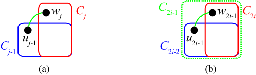
Figure 3: Illustration for Lemma 1.

We then prove that $\mathsf{TS}(C_{0},C_{r})=\mathsf{yes}$ if $\mathsf{TAR}(C_{0},C_{r},k)=\mathsf{yes}$. In this case, there exists a $\mathsf{TAR}(k)$-sequence between $C_{0}$ and $C_{r}$; let $\langle C_{0},C_{1},\dots,C_{\ell^{\prime}}\rangle$ be a shortest one, that is, $C_{\ell^{\prime}}=C_{r}$ and $\ell^{\prime}=\mathsf{dist_{TAR}}(C_{0},C_{r},k)$. Furthermore, by Lemma 10 we can assume that $|C_{2i-1}|=k+1$ and $|C_{2i}|=k$ for every $i\in\{1,2,\ldots,\ell^{\prime}/2\}$. Then, observe that $C_{2i-1}=C_{2i-2}\cup C_{2i}$ for every $i\in\{1,2,\ldots,\ell^{\prime}/2\}$, and let $C_{2i-1}=C_{2i-2}\cup\{w_{2i-1}\}=C_{2i}\cup\{u_{2i-1}\}$. (See Figure 3(b).) Since this $\mathsf{TAR}(k)$-sequence $\langle C_{0},C_{1},\dots,C_{\ell^{\prime}}\rangle$ is shortest, we have $u_{2i-1}\neq w_{2i-1}$. Furthermore, since both $u_{2i-1}$ and $w_{2i-1}$ belong to the clique $C_{2i-1}$, they are adjacent. Therefore, for every $i\in\{1,2,\ldots,\ell^{\prime}/2\}$, we have $C_{2i-2}\leftrightarrow C_{2i}$ under $\mathsf{TS}$; we replace each sub-sequence $\langle C_{2i-1},C_{2i}\rangle$ with $\langle C_{2i}\rangle$, and obtain $\mathcal{C}^{\prime\prime}=\langle C_{0},C_{2},C_{4},\ldots,C_{\ell^{\prime}}\rangle$. In this way, $\mathcal{C}^{\prime\prime}$ is a $\mathsf{TS}$-sequence from $C_{0}$ to $C_{\ell^{\prime}}=C_{r}$, and hence $\mathsf{TS}(C_{0},C_{r})=\mathsf{yes}$. Furthermore, the length of $\mathcal{C}^{\prime\prime}$ is $\ell^{\prime}/2$, and hence

$$\mathsf{dist_{TS}}(C_{0},C_{r})\leq\ell^{\prime}/2=\mathsf{dist_{TAR}}(C_{0},C_{r},k)/2.$$ (2)

By Eqs. (1) and (2) we have $\mathsf{dist_{TS}}(C_{0},C_{r})=\mathsf{dist_{TAR}}(C_{0},C_{r},k)/2$. ∎

0.A.2 Proof of Lemma 2

Since $C_{0}^{\prime}\subseteq C_{0}$ and $|C_{0}^{\prime}|=k$, we have $C_{0}\leftrightsquigarrow C_{0}^{\prime}$ under $\mathsf{TAR}(k)$ by deleting the vertices in $C_{0}\setminus C_{0}^{\prime}$ from $C_{0}$ one by one. Similarly, we have $C_{r}^{\prime}\leftrightsquigarrow C_{r}$ under $\mathsf{TAR}(k)$; recall that any reconfiguration sequence is reversible. Since $|C_{0}^{\prime}|=|C_{r}^{\prime}|=k$, by Lemma 1 we have

$$\mathsf{TS}(C_{0}^{\prime},C_{r}^{\prime})=\mathsf{TAR}(C_{0}^{\prime},C_{r}^{\prime},k).$$ (3)

We now prove that $\mathsf{TAR}(C_{0},C_{r},k)=\mathsf{yes}$ if $\mathsf{TS}(C_{0}^{\prime},C_{r}^{\prime})=\mathsf{yes}$. In this case, by Eq. (3) we have $\mathsf{TAR}(C_{0}^{\prime},C_{r}^{\prime},k)=\mathsf{yes}$ and hence $C_{0}^{\prime}\leftrightsquigarrow C_{r}^{\prime}$ under $\mathsf{TAR}(k)$. Thus, $C_{0}\leftrightsquigarrow C_{0}^{\prime}\leftrightsquigarrow C_{r}^{\prime}\leftrightsquigarrow C_{r}$ holds under $\mathsf{TAR}(k)$, and hence $\mathsf{TAR}(C_{0},C_{r},k)=\mathsf{yes}$.

We finally prove that $\mathsf{TS}(C_{0}^{\prime},C_{r}^{\prime})=\mathsf{yes}$ if $\mathsf{TAR}(C_{0},C_{r},k)=\mathsf{yes}$. In this case, since $\mathsf{TAR}(C_{0},C_{r},k)=\mathsf{yes}$, we have $C_{0}\leftrightsquigarrow C_{r}$ under $\mathsf{TAR}(k)$. Therefore, $C_{0}^{\prime}\leftrightsquigarrow C_{0}\leftrightsquigarrow C_{r}\leftrightsquigarrow C_{r}^{\prime}$ holds under $\mathsf{TAR}(k)$, and hence $\mathsf{TAR}(C_{0}^{\prime},C_{r}^{\prime},k)=\mathsf{yes}$. By Eq. (3) we then have $\mathsf{TS}(C_{0}^{\prime},C_{r}^{\prime})=\mathsf{yes}$. ∎

0.A.3 Proof of Lemma 3

We first give the following lemma, which can be obtained from the same arguments as in Lemma 10 by just shifting the threshold by one.

Lemma 11

Let $G$ be a graph, and let $C$ and $C^{\prime}$ be any pair of cliques of $G$ such that $|C|=|C^{\prime}|=k$ and $C\leftrightsquigarrow C^{\prime}$ under $\mathsf{TAR}(k-1)$. Then, there exists a shortest $\mathsf{TAR}(k-1)$-sequence $\langle C_{0},C_{1},\dots,C_{\ell}\rangle$ from $C_{0}=C$ to $C_{\ell}=C^{\prime}$ such that $|C_{2i-1}|=k-1$ and $|C_{2i}|=k$ for every $i\in\{1,2,\ldots,\ell/2\}$.

Proof of Lemma 3.

We first prove that $\mathsf{TAR}(C_{0},C_{r},k-1)=\mathsf{yes}$ if $\mathsf{TJ}(C_{0},C_{r})=\mathsf{yes}$. In this case, there exists a $\mathsf{TJ}$-sequence between $C_{0}$ and $C_{r}$; let $\langle C_{0},C_{1},\dots,C_{\ell}\rangle$ be a shortest one, that is, $C_{\ell}=C_{r}$ and $\ell=\mathsf{dist_{TJ}}(C_{0},C_{r})$. For each $j\in\{1,2,\ldots,\ell\}$, let $C_{j-1}\setminus C_{j}=\{u_{j-1}\}$ and $C_{j}\setminus C_{j-1}=\{w_{j}\}$. Then, we replace each sub-sequence $\langle C_{j}\rangle$ with $\langle C_{j-1}\setminus\{u_{j-1}\},\ C_{j}\rangle$ for each $j\in\{1,2,\ldots,\ell\}$, and obtain the following sequence $\mathcal{C}^{\prime}$ of cliques:

$$\mathcal{C}^{\prime}=\langle C_{0},\ C_{0}\setminus\{u_{0}\},\ C_{1},\ \ldots,C_{j-1}\setminus\{u_{j-1}\},\ C_{j},\ \ldots,\ C_{\ell-1}\setminus\{u_{\ell-1}\},\ C_{\ell}\rangle.$$

Notice that $C_{j-1}\setminus\{u_{j-1}\}\leftrightarrow C_{j}$ under $\mathsf{TAR}(k-1)$ for each $j\in\{1,2,\ldots,\ell\}$, because $\bigl{(}C_{j-1}\setminus\{u_{j-1}\}\bigr{)}\cup\{w_{j}\}=C_{j}$ and $\bigl{|}C_{j-1}\setminus\{u_{j-1}\}\bigr{|}=k-1$. Therefore, the sequence $\mathcal{C}^{\prime}$ above is a $\mathsf{TAR}(k-1)$-sequence from $C_{0}$ to $C_{\ell}=C_{r}$, and hence $\mathsf{TAR}(C_{0},C_{r},k-1)=\mathsf{yes}$. Furthermore, by the construction, $\mathcal{C}^{\prime}$ is of length $2\ell$. Therefore, we have

$$\mathsf{dist_{TAR}}(C_{0},C_{r},k-1)\leq 2\ell=2\cdot\mathsf{dist_{TJ}}(C_{0},C_{r}).$$ (4)

We then prove that $\mathsf{TJ}(C_{0},C_{r})=\mathsf{yes}$ if $\mathsf{TAR}(C_{0},C_{r},k-1)=\mathsf{yes}$. In this case, there exists a $\mathsf{TAR}(k-1)$-sequence between $C_{0}$ and $C_{r}$; let $\langle C_{0},C_{1},\dots,C_{\ell^{\prime}}\rangle$ be a shortest one, that is, $C_{\ell^{\prime}}=C_{r}$ and $\ell^{\prime}=\mathsf{dist_{TAR}}(C_{0},C_{r},k-1)$. Furthermore, by Lemma 11 we can assume that $|C_{2i-1}|=k-1$ and $|C_{2i}|=k$ for every $i\in\{1,2,\ldots,\ell^{\prime}/2\}$. For every $i\in\{1,2,\ldots,\ell^{\prime}/2\}$, let $C_{2i-1}=C_{2i-2}\setminus\{u_{2i-2}\}$ and $C_{2i}=C_{2i-1}\cup\{w_{2i-1}\}$. Since $\langle C_{0},C_{1},\dots,C_{\ell^{\prime}}\rangle$ is shortest, we have $u_{2i-2}\neq w_{2i-1}$. Then, for every $i\in\{1,2,\ldots,\ell^{\prime}/2\}$, we have $C_{2i-2}\leftrightarrow C_{2i}$ under $\mathsf{TJ}$; we replace each sub-sequence $\langle C_{2i-1},C_{2i}\rangle$ with $\langle C_{2i}\rangle$, and obtain $\mathcal{C}^{\prime\prime}=\langle C_{0},C_{2},C_{4},\ldots,C_{\ell^{\prime}}\rangle$. In this way, $\mathcal{C}^{\prime\prime}$ is a $\mathsf{TJ}$-sequence from $C_{0}$ to $C_{\ell^{\prime}}=C_{r}$, and hence $\mathsf{TJ}(C_{0},C_{r})=\mathsf{yes}$. Furthermore, the length of $\mathcal{C}^{\prime\prime}$ is $\ell^{\prime}/2$, and hence

$$\mathsf{dist_{TJ}}(C_{0},C_{r})\leq\ell^{\prime}/2=\mathsf{dist_{TAR}}(C_{0},C_{r},k-1)/2.$$ (5)

By Eqs. (4) and (5) we have $\mathsf{dist_{TJ}}(C_{0},C_{r})=\mathsf{dist_{TAR}}(C_{0},C_{r},k-1)/2$. ∎

0.A.4 Proof of Lemma 5

Similarly as in the proof of Lemma 2, in both cases (i) and (ii), we have $C_{0}\leftrightsquigarrow C_{0}^{\prime}$ and $C_{r}\leftrightsquigarrow C_{r}^{\prime}$ under $\mathsf{TAR}(k)$. Note that $|C_{0}^{\prime}|=|C_{r}^{\prime}|=k+1$. Then, by Lemma 3 we have

$$\mathsf{TJ}(C_{0}^{\prime},C_{r}^{\prime})=\mathsf{TAR}(C_{0}^{\prime},C_{r}^{\prime},k).$$ (6)

We first prove that $\mathsf{TAR}(C_{0},C_{r},k)=\mathsf{yes}$ if $\mathsf{TJ}(C_{0}^{\prime},C_{r}^{\prime})=\mathsf{yes}$. In this case, by Eq. (6) we have $\mathsf{TAR}(C_{0}^{\prime},C_{r}^{\prime},k)=\mathsf{yes}$, and hence $C_{0}^{\prime}\leftrightsquigarrow C_{r}^{\prime}$ under $\mathsf{TAR}(k)$. Thus, $C_{0}\leftrightsquigarrow C_{0}^{\prime}\leftrightsquigarrow C_{r}^{\prime}\leftrightsquigarrow C_{r}$ holds under $\mathsf{TAR}(k)$, and hence $\mathsf{TAR}(C_{0},C_{r},k)=\mathsf{yes}$.

We then prove that $\mathsf{TJ}(C_{0}^{\prime},C_{r}^{\prime})=\mathsf{yes}$ if $\mathsf{TAR}(C_{0},C_{r},k)=\mathsf{yes}$. In this case, since $\mathsf{TAR}(C_{0},C_{r},k)=\mathsf{yes}$, we have $C_{0}\leftrightsquigarrow C_{r}$ under $\mathsf{TAR}(k)$. Therefore, $C_{0}^{\prime}\leftrightsquigarrow C_{0}\leftrightsquigarrow C_{r}\leftrightsquigarrow C_{r}^{\prime}$ holds under $\mathsf{TAR}(k)$, and hence $\mathsf{TAR}(C_{0}^{\prime},C_{r}^{\prime},k)=\mathsf{yes}$. By Eq. (6) we then have $\mathsf{TJ}(C_{0}^{\prime},C_{r}^{\prime})=\mathsf{yes}$. ∎

0.A.5 Proof of Proposition 1

Kamiński et al. [14, Theorem 3] proved that independent set reconfiguration under $\mathsf{TAR}$ is PSPACE-complete for perfect graphs. Since the class of perfect graphs is closed under taking complements [L72], by Lemma 6 clique reconfiguration under $\mathsf{TAR}$ is PSPACE-complete for perfect graphs. Then, Theorems 3.1(b) and 3.2(b) imply that clique reconfiguration remains PSPACE-complete for perfect graphs under $\mathsf{TS}$ and $\mathsf{TJ}$, too. ∎

0.A.6 Proof of Proposition 1

From the definition, the class of cographs is closed under taking complements, and we note that the complement of a cograph can be computed in linear time [CPS85]. Bonsma [3] proved that independent set reconfiguration under $\mathsf{TAR}$ is solvable in linear time for cographs, and hence by Lemma 6 we can solve clique reconfiguration under $\mathsf{TAR}$ in linear time for cographs. Then, Theorems 3.1(a) and 3.2(a) imply that clique reconfiguration can be solved in linear time for cographs under $\mathsf{TS}$ and $\mathsf{TJ}$, too. ∎

Appendix 0.B Proofs Omitted from Section 4

0.B.1 Proof of Theorem 4.1

By Theorems 3.1(a) and 3.2(a) it suffices to give an $O(w^{2}n^{w})$-time algorithm for a $\mathsf{TAR}$-instance; recall that the reduction from $\mathsf{TS}$/$\mathsf{TJ}$ to $\mathsf{TAR}$ preserves the shortest length of reconfiguration sequences. Note that, however, the arguments for $\mathsf{TAR}$ below can be applied to the other rules $\mathsf{TS}$ and $\mathsf{TJ}$, and one can obtain algorithms directly for $\mathsf{TS}$ and $\mathsf{TJ}$ rules.

Let $(G,C_{0},C_{r},k)$ be any $\mathsf{TAR}$-instance such that $\omega(G)\leq w$. Then, the number of cliques of size at least $k$ in $G$ can be bounded by $\sum_{i=k}^{w}{n\choose i}=O(n^{w})$. We now construct a reconfiguration graph $\mathcal{R}=(\mathcal{V},\mathcal{E})$, as follows:

• each node in $\mathcal{R}$ corresponds to a clique of $G$ with size at least $k$; and

• two nodes in $\mathcal{R}$ are joined by an edge if and only if $C\leftrightarrow C^{\prime}$ holds under $\mathsf{TAR}(k)$ for the corresponding two cliques $C$ and $C^{\prime}$.

This reconfiguration graph $\mathcal{R}$ can be constructed in time $O(w^{2}n^{w})$ as follows: we first enumerate all cliques in time $O(w^{2}n^{w})$ by checking all $O(n^{w})$ vertex subsets of size at most $w$; we then add edges from each clique to its $O(w)$ subsets with one less vertex. The graph $\mathcal{R}$ has $|\mathcal{V}|=O(n^{w})$ nodes and $|\mathcal{E}|=O(wn^{w})$ edges. Then, there is a $\mathsf{TAR}(k)$-sequence between $C_{0}$ and $C_{r}$ if and only if there is a path in $\mathcal{R}$ between the two corresponding nodes. Therefore, by the breadth-first search on $\mathcal{R}$ which starts from the node corresponding to $C_{0}$, we can check if $\mathcal{R}$ has a desired path or not in time $O(|\mathcal{V}|+|\mathcal{E}|)=O(wn^{w})$. Furthermore, if such a path exists, it corresponds to a shortest $\mathsf{TAR}(k)$-sequence between $C_{0}$ and $C_{r}$. ∎

0.B.2 Proof of Proposition 3

We first compute a tree-decomposition $\mathcal{T}$ with width $5t+4$ in $O(c^{t}n)$ time, where $c$ is some constant, by using the algorithm in [1]. Additionally, we can assume that the number of bags in $\mathcal{T}$ is $O(n)$ [1]. By the definition of the tree-decomposition, every clique in $G$ is included in at least one bag of $\mathcal{T}$. Since the width of $\mathcal{T}$ is $5t+4$, each bag in $\mathcal{T}$ contains at most $5t+5$ vertices of $G$. Thus, there are at most $2^{5t+5}$ cliques in each bag of $\mathcal{T}$, and hence we can conclude that $G$ has $O(2^{5t+5}n)$ cliques. Then, the proposition follows, because we can construct a reconfiguration graph $\mathcal{R}$ in time $O(t^{2}2^{5t+5}n)$, similarly as in the proof of Theorem 4.1. ∎

0.B.3 Proof of Lemma 7

We first prove the if-part. Suppose that there is a path $\langle M_{0},M_{1},\dots,M_{\ell}\rangle$ in $\mathsf{MC}_{k}(G)$ from the node $M=M_{0}\supseteq C$ to the node $M^{\prime}=M_{\ell}\supseteq C^{\prime}$. Let $C_{0}=C$, and let $C_{j}$ be any clique in $M_{j-1}\cap M_{j}$ of size $k$ for each $j\in\{1,2,\ldots,\ell\}$; such a clique $C_{j}$ exists because $|M_{j-1}\cap M_{j}|\geq k$. Then, $C_{j-1}\leftrightsquigarrow C_{j}$ holds under $\mathsf{TAR}(k)$ because $C_{j-1}\cup C_{j}\subseteq M_{j-1}$ and hence $C_{j-1}\cup C_{j}$ forms a clique of $G$ for each $j\in\{1,2,\ldots,\ell\}$. We thus have $C=C_{0}\leftrightsquigarrow C_{1}\leftrightsquigarrow\cdots\leftrightsquigarrow C_{\ell}$ under $\mathsf{TAR}(k)$. Since both $C_{\ell}$ and $C^{\prime}$ are contained in the same maximal clique $M_{\ell}=M^{\prime}$, we have $C_{\ell}\leftrightsquigarrow C^{\prime}$ and hence $C\leftrightsquigarrow C^{\prime}$ holds under $\mathsf{TAR}(k)$.

We then prove the only-if-part. Suppose that there is a $\mathsf{TAR}(k)$-sequence $\mathcal{C}=\langle C_{0},C_{1},\ldots,C_{\ell^{\prime}}\rangle$ such that $C_{0}=C$ and $C_{\ell^{\prime}}=C^{\prime}$. Let $\mathsf{MC}_{k}(G;\mathcal{C})$ be the subgraph of $\mathsf{MC}_{k}(G)$ induced by all nodes (i.e., maximal cliques in $\mathcal{M}(G)$) that contain at least one clique in $\mathcal{C}$. Then, it suffices to show that $\mathsf{MC}_{k}(G;\mathcal{C})$ is connected; then $\mathsf{MC}_{k}(G)$ has a path from any node $M\supseteq C$ to any node $M^{\prime}\supseteq C^{\prime}$. Suppose for a contradiction that $\mathsf{MC}_{k}(G;\mathcal{C})$ is not connected. Then, there exists an index $j$ such that the cliques $C_{j-1}$ and $C_{j}$ are contained in different maximal cliques $M_{p-1}$ and $M_{p}$ which belong to different connected components in $\mathsf{MC}_{k}(G;\mathcal{C})$. In this case, $C_{j}$ must be obtained by adding a vertex $u$ to $C_{j-1}$, that is, $C_{j}=C_{j-1}\cup\{u\}$; otherwise both $C_{j-1}$ and $C_{j}$ are contained in the same maximal clique $M_{p-1}$. Since $\mathcal{C}$ is a $\mathsf{TAR}(k)$-sequence, we have $|C_{j-1}|\geq k$ and hence $|C_{j-1}\cap C_{j}|\geq k$. Then, since $C_{j-1}\subseteq M_{p-1}$ and $C_{j}\subseteq M_{p}$, we have $|M_{p-1}\cap M_{p}|\geq k$. Therefore, $M_{p-1}$ and $M_{p}$ must be joined by an edge in $\mathsf{MC}_{k}(G)$ and hence in $\mathsf{MC}_{k}(G;\mathcal{C})$. This contradicts the assumption that $M_{p-1}$ and $M_{p}$ are contained in different connected components in $\mathsf{MC}_{k}(G;\mathcal{C})$. We have thus proved that $\mathsf{MC}_{k}(G;\mathcal{C})$ is connected, and hence there is a path in $\mathsf{MC}_{k}(G)$ from any node $M\supseteq C$ to any node $M^{\prime}\supseteq C^{\prime}$. ∎

Appendix 0.C Proofs Omitted from Section 5

0.C.1 Proof of Lemma 8

We first prove the following lemma, which can be applied to any graph.

Lemma 12

For two cliques $C$ and $C^{\prime}$ in a graph $G$, suppose that $C\cup C^{\prime}$ also forms a clique in $G$. Then, $\mathsf{dist_{TAR}}(C,C^{\prime},k)=|C\vartriangle C^{\prime}|$ for every integer $k\geq\min\{|C|,|C^{\prime}|\}$. Furthermore, every clique in an arbitrary shortest $\mathsf{TAR}(k)$-sequence from $C$ to $C^{\prime}$ consists only of vertices in $C\cup C^{\prime}$.

Proof

We first prove that $\mathsf{dist_{TAR}}(C,C^{\prime},k)\leq|C\vartriangle C^{\prime}|$ holds for every integer $k\geq\min\{|C|,|C^{\prime}|\}$, by constructing a $\mathsf{TAR}(k)$-sequence between $C$ and $C^{\prime}$ of length $|C\vartriangle C^{\prime}|$, as follows: we first add the vertices in $C^{\prime}\setminus C$ to $C$ one by one, and obtain the clique $C\cup C^{\prime}$; and we then delete the vertices in $C\setminus C^{\prime}$ from $C\cup C^{\prime}$ one by one, and obtain the clique $C^{\prime}$. Since the minimum size of a clique in this sequence is $\min\{|C|,|C^{\prime}|\}$, this is a $\mathsf{TAR}(k)$-sequence for every integer $k\geq\min\{|C|,|C^{\prime}|\}$. Furthermore, the length of this $\mathsf{TAR}(k)$-sequence is $|C\vartriangle C^{\prime}|$. Therefore, we have $\mathsf{dist_{TAR}}(C,C^{\prime},k)\leq|C\vartriangle C^{\prime}|$.

We then prove that $\mathsf{dist_{TAR}}(C,C^{\prime},k)\geq|C\vartriangle C^{\prime}|$ holds for every integer $k\geq\min\{|C|,|C^{\prime}|\}$. Since $k\geq\min\{|C|,|C^{\prime}|\}$, there exists at least one $\mathsf{TAR}(k)$-sequence between $C$ and $C^{\prime}$ as explained above. Note that, in an arbitrary $\mathsf{TAR}(k)$-sequence between $C$ and $C^{\prime}$, every vertex in $C\vartriangle C^{\prime}$ must be either deleted or added at least once. Therefore, we have $\mathsf{dist_{TAR}}(C,C^{\prime},k)\geq|C\vartriangle C^{\prime}|$.

We have thus proved that $\mathsf{dist_{TAR}}(C,C^{\prime},k)=|C\vartriangle C^{\prime}|$ holds for every integer $k\geq\min\{|C|,|C^{\prime}|\}$. Consider an arbitrary shortest $\mathsf{TAR}(k)$-sequence $\mathcal{C}$ from $C$ to $C^{\prime}$. Then, every vertex in $C\vartriangle C^{\prime}$ must be either deleted or added by $\mathcal{C}$ at least once. Therefore, if $\mathcal{C}$ deletes or adds a vertex not in $C\cup C^{\prime}$, then the length of $\mathcal{C}$ is strictly greater than $|C\vartriangle C^{\prime}|$. This contradicts the assumption that $\mathcal{C}$ is shortest. We can thus conclude that every clique in an arbitrary shortest $\mathsf{TAR}(k)$-sequence from $C$ to $C^{\prime}$ consists only of vertices in $C\cup C^{\prime}$. ∎

Let $G=(V,E)$ be a graph, and let $X,Y\subseteq V$. A vertex subset $S\subseteq V$ is called an $(X,Y)$-separator of $G$ if any two vertices $x\in X\setminus S$ and $y\in Y\setminus S$ do not belong to the same component in $G-S$, where $G-S$ denotes the subgraph of $G$ induced by the vertex set $V\setminus S$.

Proof of Lemma 8.

We prove the statement by induction on the length $t$ of the unique path $(M_{0},M_{1},\ldots,M_{t})$ in $\mathcal{T}$ between $M_{0}$ and $M_{t}$.

First, consider the case where $t=0$. Then, since $C_{0}\subseteq M_{0}$ and $C_{r}\subseteq M_{t}=M_{0}$, both $C_{0}$ and $C_{r}$ are contained in the same maximal clique $M_{0}$. Therefore, $C_{0}\cup C_{r}$ forms a clique, and hence by Lemma 12 every shortest $\mathsf{TAR}(k)$-sequence passes through cliques consisting of vertices only in $M_{0}$. Thus, we set $f(i)=0$ for all $i\in\{0,1,\ldots,\ell\}$.

Next, consider the case where $t\geq 1$. We assume that $C_{r}\not\subseteq M_{0}$, because otherwise we can set $f(i)=0$ for all $i\in\{0,1,\ldots,\ell\}$ similarly as for the case $t=0$. Then, by the definition of a clique tree, $M_{0}\cap M_{1}$ forms a $(C_{0},C_{r})$-separator of $G$ (see [BP93, Lemma 4.2]).

We now claim that there exists at least one clique $C_{j}$ in the shortest $\mathsf{TAR}(k)$-sequence $\langle C_{0},C_{1},\ldots,C_{\ell}\rangle$ such that $C_{j}\subseteq M_{0}\cap M_{1}$. Suppose for a contradiction that $C_{i}\not\subseteq M_{0}\cap M_{1}$ for all $i\in\{0,1,\ldots,\ell\}$. Let $w_{i}$ be an arbitrary vertex in $C_{i}\setminus(M_{0}\cap M_{1})$ for each $i\in\{0,1,\ldots,\ell\}$. Since $\langle C_{0},C_{1},\ldots,C_{\ell}\rangle$ is a $\mathsf{TAR}(k)$-sequence, either $C_{i}\subset C_{i+1}$ or $C_{i}\supset C_{i+1}$ holds for each $i\in\{0,1,\ldots,\ell-1\}$ and hence $C_{i}\cup C_{i+1}$ forms a clique. Therefore, the vertices $w_{i}$ and $w_{i+1}$ in $C_{i}\cup C_{i+1}$ are either the same or adjacent. This implies that the subgraph of $G$ induced by $\{w_{i}\mid 0\leq i\leq\ell\}$ is connected, and hence it contains a path from $w_{0}$ to $w_{\ell}$. However, since $w_{0}\in C_{0}\setminus(M_{0}\cap M_{1})$ and $w_{\ell}\in C_{\ell}\setminus(M_{0}\cap M_{1})=C_{r}\setminus(M_{0}\cap M_{1})$, this contradicts the assumption that $M_{0}\cap M_{1}$ is a $(C_{0},C_{r})$-separator.

As the induction hypothesis, assume that the statement is true for the length $t-1\geq 0$. Let $C_{j}$ be an arbitrary clique in $\langle C_{0},C_{1},\ldots,C_{\ell}\rangle$ such that $C_{j}\subseteq M_{0}\cap M_{1}$. Note that, since $\langle C_{0},C_{1},\ldots,C_{\ell}\rangle$ is shortest, $\langle C_{0},C_{1},\ldots,C_{j}\rangle$ is a shortest $\mathsf{TAR}(k)$-sequence from $C_{0}$ to $C_{j}$. Then, since $C_{0}\cup C_{j}\subseteq M_{0}$, Lemma 12 implies that $\langle C_{0},C_{1},\ldots,C_{j}\rangle$ passes through cliques consisting of vertices only in $M_{0}$, that is,

$$C_{h}\subseteq M_{0}$$ (7)

holds for each $h\in\{0,1,\ldots,j\}$. Let $C_{i}^{\prime}=C_{j+i}$ for each $i\in\{0,1,\ldots,\ell-j\}$, and let $M_{i}^{\prime}=M_{1+i}$ for each $i\in\{0,1,\ldots,t-1\}$. Note that $\langle C_{0}^{\prime},C_{1}^{\prime},\ldots,C_{\ell-j}^{\prime}\rangle$ is a shortest $\mathsf{TAR}(k)$-sequence from $C_{0}^{\prime}=C_{j}$ to $C_{\ell-j}^{\prime}=C_{\ell}=C_{r}$. Furthermore, $C_{0}^{\prime}=C_{j}\subseteq M_{1}=M_{0}^{\prime}$, $C_{\ell-j}^{\prime}=C_{r}\subseteq M_{t}=M_{t-1}^{\prime}$ and $(M_{0}^{\prime},M_{1}^{\prime},\ldots,M_{t-1}^{\prime})$ is a path in $\mathcal{T}$ of length $t-1$. Therefore, by the induction hypothesis, there is a monotonically increasing function $f^{\prime}\colon\{0,1,\dots,\ell-j\}\to\{0,1,\dots,t-1\}$ such that

$$C_{i}^{\prime}\subseteq M_{f^{\prime}(i)}^{\prime}$$ (8)

for all $i\in\{0,1,\dots,\ell-j\}$. Now we construct a mapping $f\colon\{0,1,\dots,\ell\}\to\{0,1,\dots,t\}$, as follows:

$$f(i)=\begin{cases}0&\text{if}\ i<j,\\ f^{\prime}(i-j)+1&\text{otherwise}.\end{cases}$$

Since $f^{\prime}$ is a monotonically increasing function, $f$ is too. Furthermore, by Eqs. (7) and (8) we have $C_{i}\subseteq M_{f(i)}$ for all $i\in\{0,1,\dots,\ell\}$. Thus, $f$ satisfies the desired property. ∎

0.C.2 Proof of Lemma 9

Before giving our linear-time reduction, we give the following lemma.

Lemma 13

Suppose that $\langle C_{0},C_{1},\ldots,C_{\ell}\rangle$ is a shortest $\mathsf{TAR}(k)$-sequence in a chordal graph $G$. Let $p$ and $q$ be two indices in $\{0,1,\ldots,\ell\}$ such that $p<q$. If there is a vertex $v$ in $C_{p}\cap C_{q}$, then $v\in C_{i}$ holds for all $i\in\{p,p+1,\ldots,q\}$.

Proof

Suppose for a contradiction that the statement does not hold. We may assume without loss of generality that $v\notin C_{i}$ for every $i\in\{p+1,p+2,\ldots,q-1\}$ by setting $p$ as large as possible and $q$ as small as possible. Then, observe that $C_{p+1}\cup\{v\}=C_{p}$ and $C_{q-1}\cup\{v\}=C_{q}$.

Let $\mathcal{T}$ be a clique tree of $G$. Let $(M_{0},M_{1},\dots M_{t})$ be the path in $\mathcal{T}$ from $M_{0}$ to $M_{t}$ for any pair of maximal cliques $M_{0}\supseteq C_{0}$ and $M_{t}\supseteq C_{\ell}$. By Lemma 8 there is a monotonically increasing function $f\colon\{0,1,\dots,\ell\}\to\{0,1,\dots,t\}$ such that $C_{i}\subseteq M_{f(i)}$ for each $i\in\{0,1,\ldots,\ell\}$. Then, $f(p)\leq f(i)\leq f(q)$ for each $i\in\{p+1,p+2,\ldots,q-1\}$. Recall that, by the definition of a clique tree, the subgraph of $\mathcal{T}$ induced by $\mathcal{M}(G;v)$ is connected. Since $v\in C_{p}\cap C_{q}\subseteq M_{f(p)}\cap M_{f(q)}$, we can conclude that the vertex $v$ is contained in all maximal cliques $M_{f(p)},M_{f(p+1)},\ldots,M_{f(q)}$.

Therefore, for each $i\in\{p,p+1,\ldots,q\}$, both $C_{i}\subseteq M_{f(i)}$ and $v\in M_{f(i)}$ hold, and hence $C_{i}\cup\{v\}$ forms a clique which is contained in $M_{f(i)}$. Furthermore, $C_{i}\cup\{v\}\leftrightarrow C_{i+1}\cup\{v\}$ under $\mathsf{TAR}(k)$ for each $i\in\{p,p+1,\ldots,q-1\}$, because $C_{i}\leftrightarrow C_{i+1}$ under $\mathsf{TAR}(k)$. Recall that $C_{p+1}\cup\{v\}=C_{p}$ and $C_{q-1}\cup\{v\}=C_{q}$, and hence we replace the sub-sequence $\langle C_{p},C_{p+1},\ldots,C_{q}\rangle$ of length $q-p$ with the following sequence of length $q-p-2$:

$$\langle C_{p+1}\cup\{v\},\ C_{p+2}\cup\{v\},\ \ldots,C_{q-1}\cup\{v\}\rangle.$$

However, this contradicts the assumption that $\langle C_{0},C_{1},\ldots,C_{\ell}\rangle$ is shortest. ∎

Proof of Lemma 9.

We first add two dummy vertices $d_{0}$ and $d_{r}$ to a given chordal graph $G$. We then join $d_{0}$ with all vertices in $C_{0}$ by adding new edges to $G$; similarly, we join $d_{r}$ with all vertices in $C_{r}$. Let $G^{\prime}$ be the resulting graph. Then, $G^{\prime}$ is also a chordal graph, because the dummy vertices cannot create any new induced cycle of length more than three. Note that each of $C_{0}\cup\{d_{0}\}$ and $C_{r}\cup\{d_{r}\}$ forms a maximal clique in $G^{\prime}$. Furthermore, in the set $\mathcal{M}(G^{\prime})$ of all maximal cliques in $G$, the only maximal cliques $C_{0}\cup\{d_{0}\}$ and $C_{r}\cup\{d_{r}\}$ contain $d_{0}$ and $d_{r}$, respectively.

We now construct a clique tree $\mathcal{T}^{\prime}$ of $G^{\prime}$ in linear time [18, §15.1]. Then, $\mathcal{T}^{\prime}$ contains two nodes $M_{0}=C_{0}\cup\{d_{0}\}$ and $M_{t}=C_{r}\cup\{d_{r}\}$. Therefore, we can find the path $(M_{0},M_{1},\ldots,M_{t})$ in $\mathcal{T}^{\prime}$ in linear time. Let $H^{\prime\prime}$ be the subgraph of $G$ induced by the maximal cliques $M_{0},M_{1},\ldots,M_{t}$. Then, $H^{\prime\prime}$ is an interval graph. Furthermore, since $M_{0}=C_{0}\cup\{d_{0}\}$ and $M_{t}=C_{r}\cup\{d_{r}\}$, Lemma 8 implies that

$$\mathsf{dist_{TAR}}(H^{\prime\prime},C_{0},C_{r},k)=\mathsf{dist_{TAR}}(G^{\prime},C_{0},C_{r},k).$$ (9)

Let $H$ be the graph obtained from $H^{\prime\prime}$ by removing the dummy vertices $d_{0}$ and $d_{r}$. Since $H^{\prime\prime}$ is an interval graph, $H$ is also an interval graph. In this way, $H$ can be constructed in linear time.

Now we claim that

$$\mathsf{dist_{TAR}}(G^{\prime},C_{0},C_{r},k)=\mathsf{dist_{TAR}}(G,C_{0},C_{r},k)$$ (10)

and

$$\mathsf{dist_{TAR}}(H,C_{0},C_{r},k)=\mathsf{dist_{TAR}}(H^{\prime\prime},C_{0},C_{r},k).$$ (11)

Then, by Eqs. (9)–(11) we have $\mathsf{dist_{TAR}}(H,C_{0},C_{r},k)=\mathsf{dist_{TAR}}(G,C_{0},C_{r},k)$, as required. Note that $V(G)\vartriangle V(G^{\prime})=V(H)\vartriangle V(H^{\prime\prime})=\{d_{0},d_{r}\}$. Thus, to prove Eqs. (10) and (11), it suffices to show that there is a shortest $\mathsf{TAR}(k)$-sequence in $G^{\prime}$ (or in $H^{\prime\prime}$) from $C_{0}$ to $C_{r}$ which does not pass through any clique containing $d_{0}$ or $d_{r}$.

Let $\langle C_{0},C_{1},\ldots,C_{\ell}\rangle$ be a shortest $\mathsf{TAR}(k)$-sequence in $G^{\prime}$ (or in $H^{\prime\prime}$) from $C_{0}$ to $C_{\ell}=C_{r}$. Suppose for a contradiction that $d_{0}\in C_{i}$ holds for some $i\in\{1,2,\ldots,\ell-1\}$. (The proof for $d_{r}$ is the same.) Since $d_{0}\notin C_{0}\cup C_{\ell}$, Lemma 13 implies that there exists a pair of indices $l$ and $r$ in $\{1,2,\ldots,\ell-1\}$ such that $l\leq r$ and $d_{0}\in C_{i}$ holds for all $i\in\{l,l+1,\ldots,r\}$. Recall that $C_{0}\cup\{d_{0}\}$ is a maximal clique in $G^{\prime}$ (or in $H^{\prime\prime}$), and that no other maximal clique in $G^{\prime}$ (or in $H^{\prime\prime}$) contains $d_{0}$. This implies that $C_{i}\subseteq C_{0}\cup\{d_{0}\}$ for each $i\in\{l,l+1,\ldots,r\}$. Since $C_{l-1}=C_{l}\setminus\{d_{0}\}$ and $C_{r+1}=C_{r}\setminus\{d_{0}\}$, it follows that $C_{l-1}\cup C_{r+1}\subseteq C_{0}$ and hence $C_{l-1}\cup C_{r+1}$ forms a clique. Now, by Lemma 12 every shortest $\mathsf{TAR}(k)$-sequence from $C_{l-1}$ to $C_{r+1}$ passes through cliques consisting of vertices only in $C_{l-1}\cup C_{r+1}\subseteq C_{0}$. Since $d_{0}\not\in C_{0}$, this contradicts the assumption that $\langle C_{l-1},C_{l},\ldots,C_{r+1}\rangle$ is shortest. ∎

0.C.3 Correctness of the algorithm for interval graphs

In this subsection, we prove the correctness of the greedy algorithm in Section 5.2 and estimate its running time. For a vertex $v$ in a graph $G$, let $N(v)=\{w\in V(G)\mid vw\in E(G)\}$ and let $N[v]=N(v)\cup\{v\}$. We denote by $\deg(v)$ the degree of $v$, that is, $\deg(v)=|N(v)|$.

We first prove the correctness of Step (1) of the algorithm: if $C_{0}\not\subseteq C_{r}$ and $|C_{0}|\geq k+1$, then remove a vertex $u$ with the minimum $r$-value in $C_{0}\setminus C_{r}$ from $C_{0}$. The following lemma ensures that this operation preserves the shortest length of reconfiguration sequences.

Lemma 14

Suppose that $C_{0}\not\subseteq C_{r}$ and $|C_{0}|\geq k+1$. Let $u$ be any vertex with the minimum $r$-value in $C_{0}\setminus C_{r}$. Then,

$$\mathsf{dist_{TAR}}(C_{0},C_{r},k)=\mathsf{dist_{TAR}}(C_{0}\setminus\{u\},C_{r},k)+1.$$

Proof

First, observe that $r_{u}=0$ since $C_{0}\not\subseteq M_{1}$. Thus, $N[u]=M_{0}\subseteq N[v]$ holds for every vertex $v\in M_{0}$. Consider any clique $C$ in $H$ such that $C_{0}\leftrightarrow C$ under $\mathsf{TAR}(k)$. Then, either (i) $C=C_{0}\setminus\{v\}$ for some vertex $v\in C_{0}$, or (ii) $C=C_{0}\cup\{w\}$ for some vertex $w\in M_{0}\setminus C_{0}$; recall that $C_{0}\subseteq M_{0}$ and $C_{0}\not\subseteq M_{1}$. Therefore, it suffices to verify the following two inequalities:

$$\mathsf{dist_{TAR}}(C_{0}\setminus\{u\},C_{r},k)\leq\mathsf{dist_{TAR}}(C_{0}\setminus\{v\},C_{r},k)$$ (12)

for any vertex $v\in C_{0}$; and

$$\mathsf{dist_{TAR}}(C_{0}\setminus\{u\},C_{r},k)\leq\mathsf{dist_{TAR}}(C_{0}\cup\{w\},C_{r},k)$$ (13)

for any vertex $w\in M_{0}\setminus C_{0}$.

We first prove Eq. (12). Let $v$ be any vertex in $C_{0}\setminus\{u\}$, and let $\langle C_{1},C_{2},\ldots,C_{\ell}\rangle$ be a shortest $\mathsf{TAR}(k)$-sequence from $C_{1}=C_{0}\setminus\{v\}$ to $C_{\ell}=C_{r}$. By Lemma 13 we have $v\notin C_{i}$ for all $i\in\{1,2,\ldots,\ell\}$. On the other hand, since $u\in C_{1}\setminus C_{\ell}$, there exists an index $j\geq 1$ such that $C_{j+1}=C_{j}\setminus\{u\}$; Lemma 13 implies that $u\in C_{i}$ if and only if $i\in\{1,2,\ldots,j\}$. Then, $C_{i}^{\prime}=(C_{i}\setminus\{u\})\cup\{v\}$ forms a clique for each $i\in\{1,2,\ldots,j\}$, because $N[u]\subseteq N[v]$ for the vertex $v\in C_{0}\setminus\{u\}\subset M_{0}$. For each $i\in\{1,2,\ldots,j\}$, we replace the clique $C_{i}$ in $\langle C_{1},C_{2},\ldots,C_{\ell}\rangle$ with the clique $C_{i}^{\prime}=(C_{i}\setminus\{u\})\cup\{v\}$, and obtain the following sequence $\mathcal{C}^{\prime}$ of cliques:

$$\mathcal{C}^{\prime}=\langle C_{1}^{\prime},\ C_{2}^{\prime},\ \ldots,C_{j}^{\prime},\ C_{j+1},\ C_{j+2},\ \ldots,\ C_{\ell}\rangle.$$

Since $\langle C_{1},C_{2},\ldots,C_{\ell}\rangle$ is a $\mathsf{TAR}(k)$-sequence, we have $|C_{i}^{\prime}|=|C_{i}|\geq k$. Furthermore, $C_{i}^{\prime}\leftrightarrow C_{i+1}^{\prime}$ under $\mathsf{TAR}(k)$ for all $i\in\{1,2,\ldots,j-1\}$, since $C_{i}\leftrightarrow C_{i+1}$ under $\mathsf{TAR}(k)$. Finally, since $C_{j+1}=C_{j}\setminus\{u\}$, we have $C_{j}^{\prime}\setminus\{v\}=C_{j+1}$ and hence $C_{j}^{\prime}\leftrightarrow C_{j+1}$ under $\mathsf{TAR}(k)$. Therefore, $\mathcal{C}^{\prime}$ is a $\mathsf{TAR}(k)$-sequence from $C_{1}^{\prime}=C_{0}\setminus\{u\}$ to $C_{\ell}=C_{r}$, which has the same length $\ell$ as the shortest $\mathsf{TAR}(k)$-sequence $\langle C_{1},C_{2},\ldots,C_{\ell}\rangle$ from $C_{1}=C_{0}\setminus\{v\}$ to $C_{\ell}=C_{r}$. We have thus verified Eq. (12).

We then prove Eq. (13). Let $w$ be any vertex in $M_{0}\setminus C_{0}$, and let $\langle C_{1},C_{2},\ldots,C_{\ell}\rangle$ be a shortest $\mathsf{TAR}(k)$-sequence from $C_{1}=C_{0}\cup\{w\}$ to $C_{\ell}=C_{r}$. Let $j\in\{1,2,\ldots,\ell-1\}$ be the index such that $u\in C_{i}$ if and only if $i\in\{1,2,\ldots,j\}$. Since $r_{u}=0$, all cliques $C_{1},C_{2},\ldots,C_{j}$ are contained in $M_{0}$. Furthermore, since $C_{j+1}=C_{j}\setminus\{u\}$, we have $C_{j+1}\subseteq M_{0}$ and hence $C_{1}\cup C_{j+1}$ $(\subseteq M_{0})$ forms a clique. Then, Lemma 12 implies that $\mathsf{dist_{TAR}}(C_{1},C_{j+1},k)=|C_{1}\vartriangle C_{j+1}|$. Note that, since the sub-sequence $\langle C_{1},C_{2},\ldots,C_{j+1}\rangle$ is shortest, we have $\mathsf{dist_{TAR}}(C_{1},C_{j+1},k)=|C_{1}\vartriangle C_{j+1}|=j$. On the other hand, consider the clique $C_{1}^{\prime}=C_{0}\setminus\{u\}$; note that, since $|C_{0}|\geq k+1$, we have $|C_{1}^{\prime}|\geq k$. Since $C_{1}^{\prime},C_{j+1}\subseteq M_{0}$, the set $C_{1}^{\prime}\cup C_{j+1}$ forms a clique. Then, Lemma 12 implies that $\mathsf{dist_{TAR}}(C_{1}^{\prime},C_{j+1},k)=|C_{1}^{\prime}\vartriangle C_{j+1}|$. We now prove that

$$\mathsf{dist_{TAR}}(C_{1}^{\prime},C_{j+1},k)\leq\mathsf{dist_{TAR}}(C_{1},C_{j+1},k)=j.$$ (14)

Indeed, we show that $|C_{1}^{\prime}\vartriangle C_{j+1}|\leq|C_{1}\vartriangle C_{j+1}|$, as follows. Since $C_{1}^{\prime}=C_{1}\setminus\{u,w\}$, $u,w\in C_{1}$ and $u\notin C_{j+1}$, we have

$$|C_{1}^{\prime}\vartriangle C_{j+1}| = |C_{1}^{\prime}\cup C_{j+1}|-|C_{1}^{\prime}\cap C_{j+1}|$$

$$= |(C_{1}\setminus\{u,w\})\cup C_{j+1}|-|(C_{1}\setminus\{u,w\})\cap C_{j+1}|$$

$$= \begin{cases}(|C_{1}\cup C_{j+1}|-|\{u\}|)-(|C_{1}\cap C_{j+1}|-|\{w\}|)&\text{if }w\in C_{j+1},\\ (|C_{1}\cup C_{j+1}|-|\{u,w\}|)-|C_{1}\cap C_{j+1}|&\text{if }w\notin C_{j+1}\end{cases}$$

$$\leq |C_{1}\cup C_{j+1}|-|C_{1}\cap C_{j+1}|$$

$$= |C_{1}\vartriangle C_{j+1}|.$$

Let $\langle C_{1}^{\prime},C_{2}^{\prime},\ldots,C_{j}^{\prime},C_{j+1}\rangle$ be a shortest $\mathsf{TAR}(k)$-sequence from $C_{1}^{\prime}$ to $C_{j+1}$. Then, by Eq. (14) the length of $\langle C_{1}^{\prime},C_{2}^{\prime},\ldots,C_{j}^{\prime},C_{j+1}\rangle$ is at most $j$. We replace the sub-sequence $\langle C_{1},C_{2},\ldots,C_{j},C_{j+1}\rangle$ of length $j$ with the $\mathsf{TAR}(k)$-sequence $\langle C_{1}^{\prime},C_{2}^{\prime},\ldots,C_{j}^{\prime},C_{j+1}\rangle$. Then, $\langle C_{1}^{\prime},C_{2}^{\prime},\ldots,C_{j}^{\prime},C_{j+1},C_{j+2},\ldots,C_{\ell}\rangle$ is a $\mathsf{TAR}(k)$-sequence from $C_{1}^{\prime}=C_{0}\setminus\{u\}$ to $C_{\ell}=C_{r}$, whose length is at most $\ell-1=\mathsf{dist_{TAR}}(C_{0}\cup\{w\},C_{r},k)$. We have thus verified Eq. (13). ∎

We then prove the correctness of Step (2) of the algorithm: if no vertex can be deleted from $C_{0}$ according to Lemma 14, then add a vertex $u$ chosen by the following lemma, with preserving the shortest length of reconfiguration sequences.

Lemma 15

Assume that $C_{0}\subseteq C_{r}$ or $|C_{0}|=k$. Let $u$ be any vertex in $(C_{r}\setminus C_{0})\cap M_{0}$ if exists; otherwise, let $u$ be any vertex with the maximum $r$-value in $M_{0}\setminus C_{0}$. Then,

$$\mathsf{dist_{TAR}}(C_{0},C_{r},k)=\mathsf{dist_{TAR}}(C_{0}\cup\{u\},C_{r},k)+1.$$

Proof

Note that, if $|C_{0}|=k$, then no vertex can be deleted from $C_{0}$ due to the size constraint $k$. On the other hand, if $C_{0}\subseteq C_{r}$, then by Lemma 13 no shortest $\mathsf{TAR}(k)$-sequence from $C_{0}$ to $C_{r}$ deletes any vertex $v$ in $C_{0}$, because $v\in C_{0}\cap C_{r}$. Therefore, in any shortest $\mathsf{TAR}(k)$-sequence $\langle C_{0},C_{1},\ldots,C_{\ell}\rangle$ from $C_{0}$ to $C_{\ell}=C_{r}$, the clique $C_{1}$ must be obtained from $C_{0}$ by adding a vertex $v\in V(G)\setminus C_{0}$. Furthermore, since $C_{0}\subseteq M_{0}$, $C_{0}\not\subseteq M_{1}$ and $C_{1}=C_{0}\cup\{v\}$ is a clique, the added vertex $v$ must be in $M_{0}\setminus C_{0}$. Thus, to prove the lemma, it suffices to show that

$$\mathsf{dist_{TAR}}(C_{0}\cup\{u\},C_{r},k)\leq\mathsf{dist_{TAR}}(C_{0}\cup\{v\},C_{r},k)$$ (15)

for any vertex $v\in M_{0}\setminus C_{0}$.

Let $v$ be any vertex in $M_{0}\setminus C_{0}$, and let $\langle C_{1},C_{2},\ldots,C_{\ell}\rangle$ be a shortest $\mathsf{TAR}(k)$-sequence from $C_{1}=C_{0}\cup\{v\}$ to $C_{\ell}=C_{r}$. For each $i\in\{1,2,\ldots,\ell\}$, let

$$C_{i}^{\prime}=\begin{cases}(C_{i}\setminus\{v\})\cup\{u\}&\text{if }v\in C_{i}\text{ and }u\notin C_{i},\\ C_{i}&\text{otherwise}.\end{cases}$$ (16)

We will prove below that $\langle C_{1}^{\prime},C_{2}^{\prime},\ldots,C_{\ell}^{\prime}\rangle$ is a $\mathsf{TAR}(k)$-sequence from $C_{0}\cup\{u\}$ to $C_{r}$. Then, since $\langle C_{1}^{\prime},C_{2}^{\prime},\ldots,C_{\ell}^{\prime}\rangle$ is of length $\ell=\mathsf{dist_{TAR}}(C_{0}\cup\{v\},C_{r},k)$, Eq. (15) follows.

We first claim that $C_{1}^{\prime}=C_{0}\cup\{u\}$ and $C_{\ell}^{\prime}=C_{\ell}$. Since $v\in C_{0}\cup\{v\}=C_{1}$ and $u\not\in C_{0}\cup\{v\}=C_{1}$, we have $C_{1}^{\prime}=(C_{1}\setminus\{v\})\cup\{u\}=C_{0}\cup\{u\}$. On the other hand, if $u$ is chosen from $(C_{r}\setminus C_{0})\cap M_{0}$, then $u\in C_{r}=C_{\ell}$ and hence $C_{\ell}^{\prime}=C_{\ell}$. Otherwise, $(C_{r}\setminus C_{0})\cap M_{0}=(M_{0}\setminus C_{0})\cap C_{r}=\emptyset$ holds, and hence $v\in M_{0}\setminus C_{0}$ is not contained in $C_{r}=C_{\ell}$; we then have $C_{\ell}^{\prime}=C_{\ell}$.

We then prove that $C_{i}^{\prime}$ forms a clique of size at least $k$ for each $i\in\{1,2,\ldots,\ell\}$, and prove that $C_{i}^{\prime}\leftrightarrow C_{i+1}^{\prime}$ under $\mathsf{TAR}(k)$ for each $i\in\{1,2,\ldots,\ell-1\}$. Since $\langle C_{1},C_{2},\ldots,C_{\ell}\rangle$ is a $\mathsf{TAR}(k)$-sequence, by Eq. (16) we have $|C_{i}^{\prime}|=|C_{i}|\geq k$. Therefore, it suffices to show that $C_{i}^{\prime}\cup C_{i+1}^{\prime}$ forms a clique such that $|C_{i}^{\prime}\vartriangle C_{i+1}^{\prime}|=1$ for each $i\in\{1,2,\ldots,\ell-1\}$. This claim trivially holds for the case where both $C_{i}^{\prime}=C_{i}$ and $C_{i+1}^{\prime}=C_{i+1}$ hold, because $\langle C_{1},C_{2},\ldots,C_{\ell}\rangle$ is a $\mathsf{TAR}(k)$-sequence. By symmetry, we thus assume that $C_{i}^{\prime}=(C_{i}\setminus\{v\})\cup\{u\}$, that is, both $v\in C_{i}$ and $u\notin C_{i}$ hold. Then, there are the following three cases to consider; note that, since both $v\in C_{i}$ and $u\notin C_{i}$ hold and $C_{i}\leftrightarrow C_{i+1}$ under $\mathsf{TAR}(k)$, we do not need to consider the case where both $v\not\in C_{i+1}$ and $u\in C_{i+1}$ hold.

Case (i) $v\in C_{i+1}$ and $u\notin C_{i+1}$.

In this case, we have $C_{i+1}^{\prime}=(C_{i+1}\setminus\{v\})\cup\{u\}$. Since $C_{i}^{\prime}=(C_{i}\setminus\{v\})\cup\{u\}$ and $C_{i}\leftrightarrow C_{i+1}$ under $\mathsf{TAR}(k)$, we have $|C_{i}^{\prime}\vartriangle C_{i+1}^{\prime}|=|C_{i}\vartriangle C_{i+1}|=1$. Notice that $l_{v}=l_{u}=0$ and $r_{v}\leq r_{u}$, because $r_{u}=t$ or $u$ has the maximum $r$-value in $M_{0}\setminus C_{0}$. Therefore, $N[v]\subseteq N[u]$ holds. Then, since $C_{i}\cup C_{i+1}$ is a clique, $C_{i}^{\prime}\cup C_{i+1}^{\prime}=\bigl{(}(C_{i}\cup C_{i+1})\setminus\{v\}\bigr{)}\cup\{u\}$ forms a clique.

Case (ii) $v,u\in C_{i+1}$.

In this case, we have $C_{i+1}^{\prime}=C_{i+1}$. Recall that both $v\in C_{i}$ and $u\notin C_{i}$ hold. Then, since $v,u\in C_{i+1}$ and $C_{i}\leftrightarrow C_{i+1}$ under $\mathsf{TAR}(k)$, we have $C_{i}\cup\{u\}=C_{i+1}=C_{i+1}^{\prime}$. Since $C_{i}^{\prime}=(C_{i}\cup\{u\})\setminus\{v\}$, we thus have $C_{i}^{\prime}=C_{i+1}^{\prime}\setminus\{v\}$ and hence $|C_{i}^{\prime}\vartriangle C_{i+1}^{\prime}|=|\{v\}|=1$. Furthermore, since $C_{i+1}^{\prime}=C_{i+1}$ and $C_{i+1}$ is a clique, $C_{i}^{\prime}\cup C_{i+1}^{\prime}=C_{i+1}^{\prime}$ forms a clique.

Case (iii) $v,u\notin C_{i+1}$.

In this case, we have $C_{i+1}^{\prime}=C_{i+1}$. Recall again that both $v\in C_{i}$ and $u\notin C_{i}$ hold. Then, since $v,u\not\in C_{i+1}$ and $C_{i}\leftrightarrow C_{i+1}$ under $\mathsf{TAR}(k)$, we have $C_{i}\setminus\{v\}=C_{i+1}=C_{i+1}^{\prime}$. Since $C_{i}^{\prime}=(C_{i}\setminus\{v\})\cup\{u\}$, we thus have $C_{i}^{\prime}=C_{i+1}^{\prime}\cup\{u\}$ and hence $|C_{i}^{\prime}\vartriangle C_{i+1}^{\prime}|=|\{u\}|=1$. Then, $C_{i}^{\prime}\cup C_{i+1}^{\prime}=C_{i}^{\prime}=(C_{i}\setminus\{v\})\cup\{u\}$. Since $N[v]\subseteq N[u]$ holds and $C_{i}$ is a clique, $C_{i}^{\prime}\cup C_{i+1}^{\prime}=(C_{i}\setminus\{v\})\cup\{u\}$ forms a clique.

In this way, we have proved that $\langle C_{1}^{\prime},C_{2}^{\prime},\ldots,C_{\ell}^{\prime}\rangle$ is a $\mathsf{TAR}(k)$-sequence from $C_{0}\cup\{u\}$ to $C_{r}$, and hence Eq. (15) holds as we have mentioned above. ∎

The correctness of the greedy algorithm in Section 5.2 follows from Lemmas 14 and 15. Therefore, to complete the proof of Theorem 5.1, we now show that the algorithm runs in linear time.

Estimation of the running time.

Lemma 13 implies that each vertex is removed at most once and added at most once in any shortest $\mathsf{TAR}(k)$-sequence. Therefore, it suffices to show that each removal and addition of a vertex $u$ can be done in time $O(\deg(u))$, because $\sum_{u\in V(G)}\deg(u)=2|E(H)|$.

We first estimate the running time for Step (1) of the algorithm. We first check whether both $C_{0}\not\subseteq C_{r}$ and $|C_{0}|\geq k+1$ hold or not. These conditions can be checked in constant time by maintaining $|C_{0}|$ and $|C_{0}\cap C_{r}|$. We then find a vertex $u$ with the minimum $r$-value in $C_{0}\setminus C_{r}$; this can be done in time $O(|C_{0}|)$. After the removal of $u$, the clique $C_{0}:=C_{0}\setminus\{u\}$ may be included by some of $M_{1},M_{2},\ldots,M_{t}$; in such a case, we need to shift the indices of $M_{i}$ so that $C_{0}\subseteq M_{0}$ and $C_{0}\not\subseteq M_{1}$ hold. To do so, we compute the shift-value $i_{0}=\min\{r_{u}\mid u\in C_{0}\}$, and set $M_{i}:=M_{i-i_{0}}$ for each $i\in\{1,2,\ldots,t\}$ and $r_{w}:=r_{w}-i_{0}$ for each vertex $w\in V(H)$. However, since we just have to compute and store only the shift-value $i_{0}$ in the actual process, this post-process can be done also in time $O(|C_{0}|)$. Since $C_{0}\subseteq N[u]$, we have $|C_{0}|\leq\deg(u)+1$. Therefore, Step (1) can be executed in time $O(\deg(u))$.

We then estimate the running time for Step (2) of the algorithm. We find a vertex $u$ which either is in $(C_{r}\setminus C_{0})\cap M_{0}$ or has the maximum $r$-value in $M_{0}\setminus C_{0}$. In either case, such a vertex $u$ can be found in time $O(|M_{0}|)$. Since $M_{0}\subseteq N[u]$, the addition of $u$ can be done in time $O(\deg(u))$.

References

- [1] Bodlaender, H.L., Drange, P.G., Dregi, M.S., Fomin, F.V., Lokshtanov, D., Pilipczuk, M.: An -approximation algorithm for treewidth. Proc. of FOCS 2013, pp. 499–508 (2013)
- [2] Bonsma, P., Cereceda, L.: Finding paths between graph colourings: PSPACE-completeness and superpolynomial distances. Theoretical Computer Science 410, pp. 5215–5226 (2009)
- [3] Bonsma, P.: Independent set reconfiguration in cographs. Proc. of WG 2014, LNCS 8747, pp. 105–116 (2014)
- [4] Brandstädt, A., Le, V.B., Spinrad, J.P.: Graph Classes: A Survey, SIAM (1999)
- [5] da Silva, M.V.G., Vuković, K.: Triangulated neighborhoods in even-hole-free graphs. Discrete Mathematics, 307:1065–1073, 2007.
- [6] Fulkerson, D.R., Gross., O.A.: Incidence matrices and interval graphs. Pacific J. Mathematics 15, pp. 835–855 (1965)
- [7] Garey, M.R., Johnson, D.S.: Computers and Intractability: A Guide to the Theory of NP-Completeness. Freeman, San Francisco (1979)
- [8] Gavril, F.: The intersection graphs of subtrees in trees are exactly the chordal graphs. J. Combinatorial Theory, Series B 16, pp. 47–56 (1974)
- [9] Gilmore, P.C., Hoffman, A.J.: A characterization of comparability graphs and of interval graphs. Canadian J. Mathematics 16, pp. 539–548 (1964)
- [10] Gopalan, P., Kolaitis, P.G., Maneva, E.N., Papadimitriou, C.H.: The connectivity of Boolean satisfiability: computational and structural dichotomies. SIAM J. Computing 38, pp. 2330–2355 (2009)
- [11] Hearn, R.A., Demaine, E.D.: PSPACE-completeness of sliding-block puzzles and other problems through the nondeterministic constraint logic model of computation. Theoretical Computer Science 343, pp. 72–96 (2005)
- [12] Ito, T., Demaine, E.D., Harvey, N.J.A., Papadimitriou, C.H., Sideri, M., Uehara, R., Uno, Y.: On the complexity of reconfiguration problems. Theoretical Computer Science 412, pp. 1054–1065 (2011)
- [13] Ito, T., Nooka, H., Zhou, X.: Reconfiguration of vertex covers in a graph. To appear in Proc. of IWOCA 2014.
- [14] Kamiński, M., Medvedev, P., Milani, M.: Complexity of independent set reconfigurability problems. Theoretical Computer Science 439, pp. 9–15 (2012)
- [15] Lee, C., Oum, S.: Number of cliques in graphs with forbidden subdivision. arXiv:1407.7707 (2014)
- [16] Mouawad, A.E., Nishimura, N., Raman, V.: Vertex cover reconfiguration and beyond. Proc. of ISAAC 2014, LNCS 8889, pp. 452–463 (2014)
- [17] Robertson, N., Seymour, P.D.: Graph minors. II. Algorithmic aspects of tree-width. J. Algorithms 7, pp. 309–322 (1986)
- [18] Spinrad, J.P.: Efficient Graph Representations. American Mathematical Society (2003)
- [19] Tsukiyama, S., Ide, M., Ariyoshi, H., Shirakawa, I.: A new algorithm for generating all the maximal independent sets. SIAM J. Computing 6, pp. 505–517 (1977)
- [20] Uehara, R., Uno, Y.: On computing longest paths in small graph classes. International J. Foundations of Computer Science 18, pp. 911–930 (2007)
- [21] van den Heuvel, J.: The complexity of change. Surveys in Combinatorics 2013, London Mathematical Society Lecture Notes Series 409 (2013).
- [22] Wrochna, M.: Reconfiguration in bounded bandwidth and treedepth. arXiv:1405.0847 (2014)

References

- [BP93] Blair, J.R.S., Peyton, B.: An introduction to chordal graphs and clique trees. Graph Theory and Sparse Matrix Computation 56, pp. 1–29 (1993)
- [CPS85] Corneil, D.G., Perl, Y., Stewart, L.K.: A linear recognition algorithm for cographs. SIAM J. Computing 14, pp. 926–934 (1985)
- [L72] Lovász, L.: Normal hypergraphs and the perfect graph conjecture. Discrete Mathematics 2, pp. 253–267 (1972)