Probe of anomalous quartic $WWZ\gamma$ couplings in photon-photon collisions

Abstract

In this paper, we examine the potentials of the processes $\gamma\gamma\rightarrow W^{+}W^{-}Z$ and $e^{+}e^{-}\rightarrow e^{+}\gamma^{*}\gamma^{*}e^{-}\rightarrow e^{+}W^{+}W^{-}Ze^{-}$ at the CLIC with $\sqrt{s}=0.5,1.5$ and $3$ TeV to investigate anomalous quartic $WWZ\gamma$ couplings by two different CP-violating and CP-conserving effective Lagrangians. We find $95\%$ confidence level sensitivities on the anomalous coupling parameters at the three CLIC energies and various integrated luminosities. The best sensitivities obtained from the process $\gamma\gamma\rightarrow W^{+}W^{-}Z$ on the anomalous $\frac{k_{0}^{W}}{\Lambda^{2}}$, $\frac{k_{c}^{W}}{\Lambda^{2}}$ and $\frac{k_{2}^{m}}{\Lambda^{2}}$ couplings defined by CP-conserving effective Lagrangians are $[-1.73;\,1.73]\times 10^{-7}$ GeV^-2, $[-2.44;\,2.44]\times 10^{-7}$ and $[-1.89;\,1.89]\times 10^{-7}$ GeV^-2, while $\frac{a_{n}}{\Lambda^{2}}$ coupling determined by CP-violating effective Lagrangians is obtained as $[-1.74;\,1.74]\times 10^{-7}$ GeV^-2. In addition, the best sensitivities derived on $\frac{k_{0}^{W}}{\Lambda^{2}}$, $\frac{k_{c}^{W}}{\Lambda^{2}}$ and $\frac{k_{2}^{m}}{\Lambda^{2}}$ and $\frac{a_{n}}{\Lambda^{2}}$ from the process $e^{+}e^{-}\rightarrow e^{+}\gamma^{*}\gamma^{*}e^{-}\rightarrow e^{+}W^{+}W^{-}Ze^{-}$ are obtained as $[-1.09;\,1.09]\times 10^{-6}$ GeV^-2, $[-1.54;\,1.54]\times 10^{-6}$ GeV^-2, $[-1.18;\,1.18]\times 10^{-6}$ and $[-1.04;\,1.04]\times 10^{-6}$ GeV^-2, respectively.

I Introduction

Gauge boson self-couplings are completely defined by the non-abelian $SU(2)\times U(1)$ gauge symmetry of the Standard Model (SM), thus direct search for these couplings are extremely significant in understanding the gauge structure of the SM. However, the possible deviation from the SM predictions of gauge boson self-couplings would be a sign for the presence of new physics beyond the SM. Probe of the new physics in a model independent way by means of the effective Lagrangian approach is often a common way. In this approach, anomalous quartic gauge boson couplings are described by means of high-dimensional effective operators and they do not cause anomalous trilinear gauge boson couplings. Therefore, anomalous quartic gauge boson couplings can be independently investigated from any trilinear gauge boson couplings.

In the literature, the anomalous quartic $WWZ\gamma$ couplings are usually investigated by two different dimension 6 effective Lagrangians that keep custodial $SU(2)_{c}$ symmetry and local $U(1)_{QED}$ symmetry. The first is CP-violating effective Lagrangian. It is defined by lag1

$$\textit{L}_{n}=\frac{i\pi\alpha}{4\Lambda^{2}}a_{n}\epsilon_{ijk}W_{\mu\alpha}^{(i)}W_{\nu}^{(j)}W^{(k)\alpha}F^{\mu\nu}$$ (1)

where $F^{\mu\nu}$ is the tensor for electromagnetic field strength, $\alpha=\frac{e^{2}}{4\pi}$ is the fine structure constant, $a_{n}$ is the dimensionless anomalous quartic coupling constant and $\Lambda$ is represented the energy scale of new physics. The anomalous $WWZ\gamma$ vertex function obtained from effective Lagrangian in Eq. $1$ is given in Appendix.

Secondly, we apply the formalism of Ref. lhc to examine CP-conserving effective Lagrangian. As can be seen from Eq. 5 in Ref. lhc , there are fourteen effective photonic operators related to the anomalous quartic gauge couplings. These operators are identified by fourteen independent couplings $k_{0,c}^{w,b,m},k_{1,2,3}^{w,m}$ and $k_{1,2}^{b}$. However, the effective interactions in these operators can be expressed in terms of independent Lorentz structures. For example, the $WW\gamma\gamma$ and $ZZ\gamma\gamma$ interactions can be parameterized in terms of four independent Lorentz structures,

$$\textit{W}_{0}^{\gamma} = \frac{-e^{2}g^{2}}{2}F_{\mu\nu}F^{\mu\nu}W^{+\alpha}W_{\alpha}^{-},$$ (2)

$$\textit{W}_{c}^{\gamma} = \frac{-e^{2}g^{2}}{4}F_{\mu\nu}F^{\mu\alpha}(W^{+\nu}W_{\alpha}^{-}+W^{-\nu}W_{\alpha}^{+}),$$ (3)

$$\textit{Z}_{0}^{\gamma} = \frac{-e^{2}g^{2}}{4\textmd{cos}^{2}\,\theta_{W}}F_{\mu\nu}F^{\mu\nu}Z^{\alpha}Z_{\alpha},$$ (4)

$$\textit{Z}_{c}^{\gamma} = \frac{-e^{2}g^{2}}{4\textmd{cos}^{2}\,\theta_{W}}F_{\mu\nu}F^{\mu\alpha}Z^{\nu}Z_{\alpha}.$$ (5)

Also, among them two are related to $ZZZ\gamma$ operators:

$$\textit{Z}_{0}^{Z} = \frac{-e^{2}g^{2}}{2\textmd{cos}^{2}\,\theta_{W}}F_{\mu\nu}Z^{\mu\nu}Z^{\alpha}Z_{\alpha},$$ (6)

$$\textit{Z}_{c}^{Z} = \frac{-e^{2}g^{2}}{2\textmd{cos}^{2}\,\theta_{W}}F_{\mu\nu}Z^{\mu\alpha}Z^{\nu}Z_{\alpha}.$$ (7)

The remaining $WWZ\gamma$ interactions are given as follows

$$\textit{W}_{0}^{Z} = -e^{2}g^{2}F_{\mu\nu}Z^{\mu\nu}W^{+\alpha}W_{\alpha}^{-},$$ (8)

$$\textit{W}_{c}^{Z} = -\frac{e^{2}g^{2}}{2}F_{\mu\nu}Z^{\mu\alpha}(W^{+\nu}W_{\alpha}^{-}+W^{-\nu}W_{\alpha}^{+})$$ (9)

$$\textit{W}_{1}^{Z} = -\frac{eg_{z}g^{2}}{2}F^{\mu\nu}(W_{\mu\nu}^{+}W_{\alpha}^{-}Z^{\alpha}+W_{\mu\nu}^{-}W_{\alpha}^{+}Z^{\alpha})$$ (10)

$$\textit{W}_{2}^{Z} = -\frac{eg_{z}g^{2}}{2}F^{\mu\nu}(W_{\mu\alpha}^{+}W^{-\alpha}Z_{\nu}+W_{\mu\alpha}^{-}W^{+\alpha}Z_{\nu})$$ (11)

$$\textit{W}_{3}^{Z} = -\frac{eg_{z}g^{2}}{2}F^{\mu\nu}(W_{\mu\alpha}^{+}W^{-}_{\nu}Z^{\alpha}+W_{\mu\alpha}^{-}W_{\nu}^{+}Z^{\alpha})$$ (12)

with $g=e/s_{W}$, $g_{z}=e/s_{W}c_{W}$ and $V_{\mu\nu}=\partial_{\mu}V_{\nu}-\partial_{\nu}V_{\mu}$ where $s_{W}=\textmd{sin}\,\theta_{W}$, $c_{W}=\textmd{cos}\,\theta_{W}$ and $V=W^{\pm},Z$. The anomalous vertex functions obtained through the CP-conserving anomalous $WWZ\gamma$ interactions in Eqs. ($8$)-($12$) are given in Appendix.

Therefore, the fourteen effective photonic operators related to the anomalous quartic gauge couplings can be appropriately rewritten in terms of the above independent Lorentz structures

$$\textit{L}= \frac{k_{0}^{\gamma}}{\Lambda^{2}}(\textit{Z}_{0}^{\gamma}+\textit{W}_{0}^{\gamma})+\frac{k_{c}^{\gamma}}{\Lambda^{2}}(\textit{Z}_{c}^{\gamma}+\textit{W}_{c}^{\gamma})+\frac{k_{1}^{\gamma}}{\Lambda^{2}}\textit{Z}_{0}^{\gamma}$$ (13)

$$+\frac{k_{23}^{\gamma}}{\Lambda^{2}}\textit{Z}_{c}^{\gamma}+\frac{k_{0}^{Z}}{\Lambda^{2}}\textit{Z}_{0}^{Z}+\frac{k_{c}^{Z}}{\Lambda^{2}}\textit{Z}_{c}^{Z}+\sum_{i}\frac{k_{i}^{W}}{\Lambda^{2}}\textit{W}_{i}^{Z}$$

where the coefficients that parametrise the strength of the anomalous quartic gauge couplings are expressed as

$$k_{j}^{\gamma}=k_{j}^{w}+k_{j}^{b}+k_{j}^{m}\,\,\,\,\,\,\,\,\,\,\,\,\,\,\,\,(j=0,c,1)$$ (14)

$$k_{23}^{\gamma}=k_{2}^{w}+k_{2}^{b}+k_{2}^{m}+k_{3}^{w}+k_{3}^{m}$$ (15)

$$k_{0}^{Z}=\frac{c_{W}}{s_{W}}(k_{0}^{w}+k_{1}^{w})-\frac{s_{W}}{c_{W}}(k_{0}^{b}+k_{1}^{b})+c_{zw}(k_{0}^{m}+k_{1}^{m}),$$ (16)

$$k_{c}^{Z}=\frac{c_{W}}{s_{W}}(k_{c}^{w}+k_{2}^{w}+k_{3}^{w})-\frac{s_{W}}{c_{W}}(k_{c}^{b}+k_{2}^{b})+c_{zw}(k_{c}^{m}+k_{2}^{m}+k_{3}^{m}),$$ (17)

$$k_{0}^{W}=\frac{c_{W}}{s_{W}}k_{0}^{w}-\frac{s_{W}}{c_{W}}k_{0}^{b}+c_{zw}k_{0}^{m},$$ (18)

$$k_{c}^{W}=\frac{c_{W}}{s_{W}}k_{c}^{w}-\frac{s_{W}}{c_{W}}k_{c}^{b}+c_{zw}k_{c}^{m},$$ (19)

$$k_{j}^{W}=k_{j}^{w}+\frac{1}{2}k_{j}^{m}\,\,\,\,\,\,\,\,\,\,\,\,\,\,\,\,(j=1,2,3).$$ (20)

where $c_{zw}=(c_{W}^{2}-s_{W}^{2})/(2c_{W}s_{W})$.

For this study, we take care of the five coefficients $k_{i}^{W}$($i=0,c,1,2,3$) defined in Eqs. ($18$)-($20$) corresponding to the $WWZ\gamma$ vertex. However, these parameters are correlated with those coupling constants that describe $WW\gamma\gamma,ZZ\gamma\gamma$ and $ZZZ\gamma$ couplings lhc . Thus, the anomalous $WWZ\gamma$ coupling should be dissociated from the other anomalous quartic couplings to obtain the only non-vanishing $WWZ\gamma$ vertex. For the non-vanishing of the only $WWZ\gamma$ vertex, we can apply additional restrictions on $k_{i}^{j}$ parameters. One of the possible restrictions, proposed in lag3 , to verify this is to set $k_{2}^{m}=-k_{3}^{m}$ and other parameters($k_{0,c}^{w,b,m},k_{1,2,3}^{w},k_{1}^{m}$ and $k_{1,2}^{b}$) to zero. As a result of this choice, Eq. ($13$) reduces to only non-vanishing $WWZ\gamma$ couplings as follows

$$\textit{L}_{eff}=\frac{k_{2}^{m}}{2\Lambda^{2}}(W_{2}^{Z}-W_{3}^{Z}).$$ (21)

The current experimental sensitivities on $a_{n}/\Lambda^{2}$ parameter derived from CP-violating effective Lagrangian through the process $e^{+}e^{-}\rightarrow W^{+}W^{-}\gamma$ at the LEP are obtained by L3, OPAL and DELPHI collaborations. These are

$$\textit{L3}:-0.14\,\textmd{GeV}^{-2}<\frac{a_{n}}{\Lambda^{2}}<0.13\,\textmd{GeV}^{-2},$$ (22)

$$\textit{OPAL}:-0.16\,\textmd{GeV}^{-2}<\frac{a_{n}}{\Lambda^{2}}<0.15\,\textmd{GeV}^{-2},$$ (23)

$$\textit{DELPHI}:-0.18\,\textmd{GeV}^{-2}<\frac{a_{n}}{\Lambda^{2}}<0.14\,\textmd{GeV}^{-2}$$ (24)

at $95\%$ confidence level lep1 ; lep2 ; lep3 .

Besides, the CERN LHC provides current experimental sensitivities on only $\frac{k_{0}^{W}}{\Lambda^{2}}$ and $\frac{k_{c}^{W}}{\Lambda^{2}}$ couplings given in Eqs. ($18$)-($19$) which are related to the anomalous quartic $WWZ\gamma$ couplings within CP-conserving effective Lagrangians sınır . The results obtained for these couplings at $95\%$ C. L. through the process $q\overline{q}^{\prime}\rightarrow W(\rightarrow\ell\nu)Z(\rightarrow jj)\gamma$ at $\sqrt{s}=8$ TeV with an integrated luminosity of $19.3$ fb^-1 are given as follows

$$-1.2\times 10^{-5}\textmd{GeV}^{-2}<\frac{k_{0}^{W}}{\Lambda^{2}}<1\times 10^{-5}\textmd{GeV}^{-2}$$ (25)

and

$$-1.8\times 10^{-5}\textmd{GeV}^{-2}<\frac{k_{c}^{W}}{\Lambda^{2}}<1.7\times 10^{-5}\textmd{GeV}^{-2}.$$ (26)

There have been many studies for anomalous quartic $WWZ\gamma$ couplings at linear and hadron colliders. The linear $e^{+}e^{-}$ colliders and their operating modes of $e\gamma$ and $\gamma\gamma$ have been investigated through the processes $e^{+}e^{-}\rightarrow W^{+}W^{-}Z,W^{+}W^{-}\gamma$ lin ; lag3 ; linb ; linc ; lind ; line , $e^{+}e^{-}\rightarrow e^{+}\gamma^{*}e^{-}\rightarrow e^{+}W^{-}Z\nu_{e}$ mur , $e\gamma\rightarrow W^{+}W^{-}e,\nu_{e}W^{-}Z$ lag1 ; lin2 and $\gamma\gamma\rightarrow W^{+}W^{-}Z$ lin3 ; lin4 . In addition, a detailed analysis of anomalous $WWZ\gamma$ couplings at the LHC have been studied via the processes $pp\rightarrow$ $WZ\gamma$ lhc ; lhc1 and $pp\rightarrow p\gamma^{*}p\rightarrow pWZqX$ mur1 . The photonic quartic $WW\gamma\gamma$ and $ZZ\gamma\gamma$ couplings are examined in photon-photon reactions, i.e. $pp\to p\gamma^{*}\gamma^{*}p\to pW^{+}W^{-}p$ Pierzchala:2008xc ; Chapon:2009hh ; deFavereaudeJeneret:2009db for $WW\gamma\gamma$ couplings and $pp\to p\gamma^{*}\gamma^{*}p\to pZZp$ Chapon:2009hh ; Gupta:2011be .

The LHC is anticipated to answer some of the unsolved questions of particle physics. However, it may not provide high precision measurements due to the remnants remaining after the collision of the proton beams. A linear $e^{+}e^{-}$ collider with high luminosity and energy is the best option to complement and to extend the LHC physics program. The CLIC is one of the most popular linear colliders, planned to carry out $e^{+}e^{-}$ collisions at energies from $0.5$ TeV to $3$ TeV clic . To have its high luminosity and energy is quite important with regards to new physics research beyond the SM. Since the anomalous quartic $WWZ\gamma$ couplings described through CP-violating and CP-conserving effective Lagrangians have dimension-6, they have very strong energy dependences. Thus, the anomalous cross section containing the $WWZ\gamma$ vertex has a higher energy than the SM cross section. In addition, the future linear collider will possibly generate a final state with three or more massive gauge bosons. Hence, it will have a great potential to examine anomalous quartic gauge boson couplings.

Another possibility expected for the linear colliders is to operate this machine as $\gamma\gamma$ and $\gamma e$ colliders. This can be performed by converting the incoming leptons into intense beams of high-energy photons las1 ; las2 . On the other hand, $\gamma^{*}\gamma^{*}$ and $\gamma^{*}e$ processes at the linear colliders arise from quasi-real photon emitted from the incoming $e^{+}$ or $e^{-}$ beams. Hence, $\gamma^{*}\gamma^{*}$ and $\gamma^{*}e$ processes are more realistic than $\gamma\gamma$ and $\gamma e$ processes. The photons in these processes are defined by the Equivalent Photon Approximation (EPA) Brodsky:1971ud ; Terazawa:1973tb ; es1 ; es2 ; es3 . In the EPA, the quasi-real photons are scattered at very small angles from the beam pipe, so they have low virtuality. For this reason, they are supposed to be almost real. Moreover, the EPA has a lot of advantages: First, it provides the skill to reach crude numerical predictions via simple formulae. In addition, it may principally ease the experimental analysis because it enables one to achieve directly a rough cross section for $\gamma^{*}\gamma^{*}\rightarrow X$ process via the examination of the main process $e^{+}e^{-}\rightarrow e^{+}Xe^{-}$. Here, $X$ represents objects produced in the final state. The production of high mass objects is specially interesting at the linear colliders. Furthermore, the production rate of massive objects is limited by the photon luminosity at high invariant mass.

In conclusion, these processes have a very clean experimental environment, since they have no interference with weak and strong interactions. Up to now, the photon-induced processes for the new physics searches were investigated through the EPA at the LEP, Tevatron, LHC and CLIC in literature a1 ; a2 ; a3 ; a4 ; a5 ; a6 ; a7 ; a8 ; a9 ; a10 ; a11 ; a12 ; a13 ; a14 ; a16 ; a17 ; a18 ; a19 ; a20 ; a21 ; a22 ; a23 ; a24 ; a25 ; a26 ; a27 ; a28 ; a29 ; a30 ; murc1 ; murc2 ; murc3 ; murc4 ; murc5 .

II CROSS SECTIONS AND NUMERICAL ANALYSIS

All numerical calculations in this study were evaluated using the computer package CalcHEP calc by embedding the anomalous $WWZ\gamma$ interaction vertices defined through CP-violating [Eq.($1$)] and CP-conserving [Eqs. ($8$)-($12$)] effective operators. The total cross sections for two processes $\gamma\gamma\rightarrow W^{+}W^{-}Z$ and $e^{+}e^{-}\rightarrow e^{+}\gamma^{*}\gamma^{*}e^{-}\rightarrow e^{+}W^{+}W^{-}Ze^{-}$ in terms of $k_{i}^{W}$ ($i=0,c$) couplings can be given by

$$\sigma_{tot}=\sigma_{SM}+\sum_{i}\frac{k_{i}^{W}}{\Lambda^{2}}\sigma_{int}^{i}+\sum_{i,j}\frac{k_{i}^{W}k_{j}^{W}}{\Lambda^{4}}\sigma_{ano}^{ij}.$$ (27)

In addition, the total cross sections containing $k_{2}^{m}$ couplings are obtained as follows

$$\sigma_{tot}=\sigma_{SM}+\frac{k_{2}^{m}}{\Lambda^{2}}\sigma_{int}+\frac{(k_{2}^{m})^{2}}{\Lambda^{4}}\sigma_{ano}.$$ (28)

Finally, the total cross sections including $a_{n}$ couplings can be written by

$$\sigma_{tot}=\sigma_{SM}+\frac{a_{n}^{2}}{\Lambda^{4}}\sigma_{ano}$$ (29)

where $\sigma_{SM}$ is the SM cross section, $\sigma_{int}$ is the interference terms between SM and the anomalous contribution, and $\sigma_{ano}$ is the pure anomalous contribution. The interference terms in total cross sections given in Eqs. $(27)$-$(28)$ related to CP-conserving effective Lagrangians are negligibly small compared to pure anomalous terms. Nevertheless, we took into account the effect of all interference term in the numerical calculations. However, the total cross section depends only on the quadratic function of $a_{n}$ anomalous coupling defined by CP-violating effective Lagrangians, since anomalous coupling $a_{n}$ does not interfere with the SM amplitude.

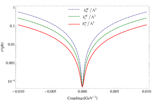
Figure 2: The total cross sections as function of anomalous $\frac{k_{0}^{W}}{\Lambda^{2}}$, $\frac{k_{c}^{W}}{\Lambda^{2}}$ and $\frac{k_{2}^{m}}{\Lambda^{2}}$ couplings for the process $e^{+}e^{-}\rightarrow e^{+}\gamma^{*}\gamma^{*}e^{-}\rightarrow e^{+}W^{+}W^{-}Ze^{-}$ at the CLIC with $\sqrt{s}=0.5$ TeV.

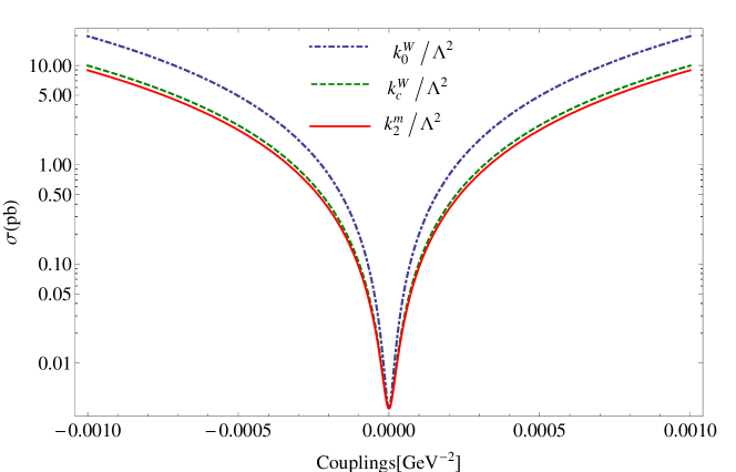
Figure 3: The same as Fig. 2 but for $\sqrt{s}=1.5$ TeV.

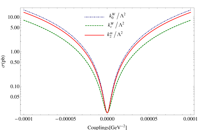
Figure 4: The same as Fig. 2 but for $\sqrt{s}=3$ TeV.

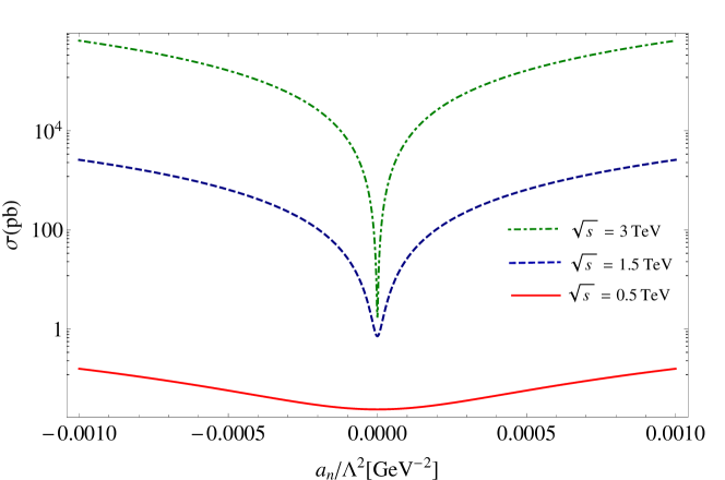
Figure 5: The total cross sections as function of anomalous $\frac{a_{n}}{\Lambda^{2}}$ coupling for the process $e^{+}e^{-}\rightarrow e^{+}\gamma^{*}\gamma^{*}e^{-}\rightarrow e^{+}W^{+}W^{-}Ze^{-}$ at the CLIC with $\sqrt{s}=0.5,1.5$ and $3$ TeV.

The quasi-real photons emitted from both lepton beams collide with each other, and the process $\gamma^{*}\gamma^{*}\rightarrow W^{+}W^{-}Z$ is generated. The process $\gamma^{*}\gamma^{*}\rightarrow W^{+}W^{-}Z$ participates as a subprocess in the main process $e^{+}e^{-}\rightarrow e^{+}\gamma^{*}\gamma^{*}e^{-}\rightarrow e^{+}W^{+}W^{-}Ze^{-}$. A schematic diagram representing the main process is given in Fig. 1. When calculating the total cross sections for this process, we used the equivalent photon spectrum described by the EPA which is embedded in CalcHEP. The total cross sections of the process $e^{+}e^{-}\rightarrow e^{+}\gamma^{*}\gamma^{*}e^{-}\rightarrow e^{+}W^{+}W^{-}Ze^{-}$ as functions of anomalous $\frac{k_{0}^{W}}{\Lambda^{2}}$, $\frac{k_{c}^{W}}{\Lambda^{2}}$, $\frac{k_{2}^{m}}{\Lambda^{2}}$ at $\sqrt{s}$=0.5, 1.5 and 3 TeV are shown in Figs. 2-4, respectively. Dependence of the $e^{+}e^{-}\rightarrow e^{+}\gamma^{*}\gamma^{*}e^{-}\rightarrow e^{+}W^{+}W^{-}Ze^{-}$ cross section on the anomalous $\frac{a_{n}}{\Lambda^{2}}$ couplings at the same three center-of-mass energies are given in Fig. 5. Here, we assume that only one of the anomalous couplings deviate from the SM at any given time. We can see from Figs. 2-4 that the deviation from SM of the anomalous cross sections including $\frac{k_{0}^{W}}{\Lambda^{2}}$ is larger than those of containing $\frac{k_{c}^{W}}{\Lambda^{2}}$ and $\frac{k_{2}^{m}}{\Lambda^{2}}$. Hence, sensitivities on the coupling $\frac{k_{0}^{W}}{\Lambda^{2}}$ are expected to be more restrictive than the sensitivities on $\frac{k_{c}^{W}}{\Lambda^{2}}$ and $\frac{k_{2}^{m}}{\Lambda^{2}}$.

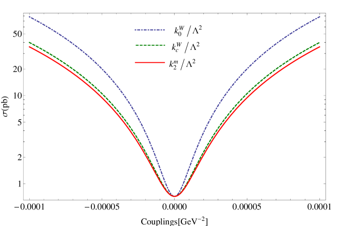
Figure 7: The same as Fig. 6 but for $\sqrt{s}=1.5$ TeV.

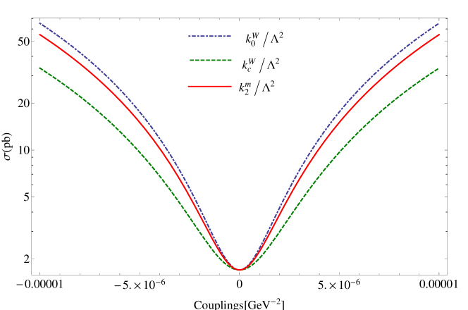
Figure 8: The same as Fig. 6 but for $\sqrt{s}=3$ TeV.

The total cross section for the $\gamma\gamma\rightarrow W^{+}W^{-}Z$ process has been calculated by using real photon spectrum produced by Compton backscattering of laser beam off the high energy electron beam. In Figs. 6-8, we plot the total cross section of the process $\gamma\gamma\rightarrow W^{+}W^{-}Z$ as a function of anomalous couplings for $\sqrt{s}=0.5,1.5$ and $3$ TeV energies. The total cross section depending on the anomalous $\frac{a_{n}}{\Lambda^{2}}$ of the process $\gamma\gamma\rightarrow W^{+}W^{-}Z$ for the three center of mass energies are plotted in Fig. 9.

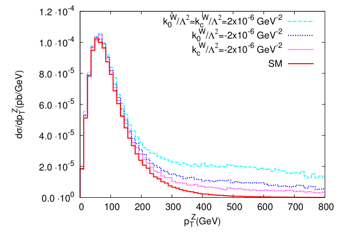
Figure 10: The transverse momentum distributions of $Z$ boson in the final states using anomalous $\frac{k_{0}^{W}}{\Lambda^{2}}$ and $\frac{k_{c}^{W}}{\Lambda^{2}}$ couplings for the processes $e^{+}e^{-}\rightarrow e^{+}\gamma^{*}\gamma^{*}e^{-}\rightarrow e^{+}W^{+}W^{-}Ze^{-}$ at $\sqrt{s}=3$ TeV.

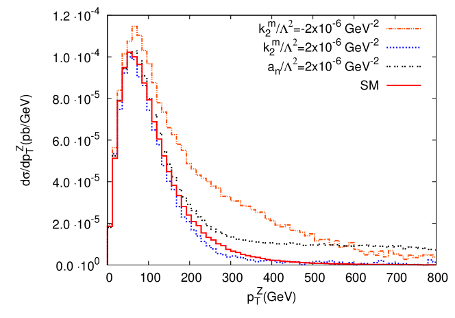
Figure 11: The transverse momentum distributions of $Z$ boson in the final states using anomalous $\frac{k_{2}^{m}}{\Lambda^{2}}$ and $\frac{a_{n}}{\Lambda^{2}}$ couplings for the processes $e^{+}e^{-}\rightarrow e^{+}\gamma^{*}\gamma^{*}e^{-}\rightarrow e^{+}W^{+}W^{-}Ze^{-}$ at $\sqrt{s}=3$ TeV.

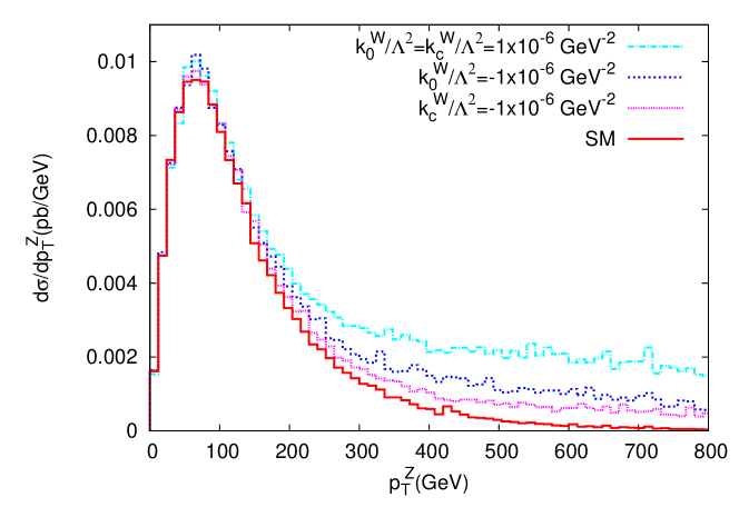
Figure 12: The transverse momentum distributions of $Z$ boson in the final states using anomalous $\frac{k_{0}^{W}}{\Lambda^{2}}$ and $\frac{k_{c}^{W}}{\Lambda^{2}}$ couplings for the processes $\gamma\gamma\rightarrow W^{+}W^{-}Z$ at $\sqrt{s}=3$ TeV.

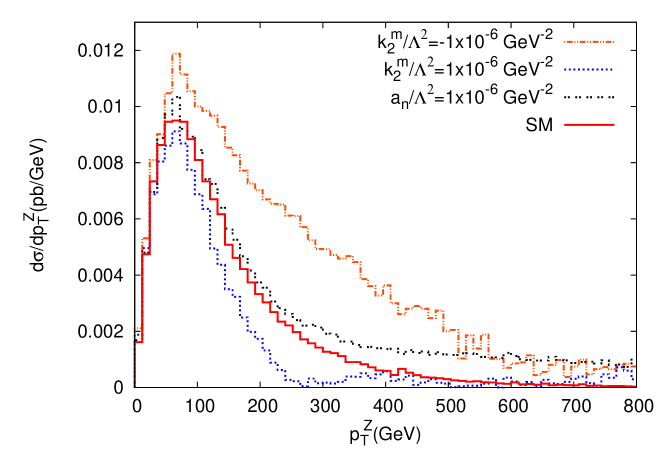
Figure 13: The transverse momentum distributions of $Z$ boson in the final states using anomalous $\frac{k_{2}^{m}}{\Lambda^{2}}$ and $\frac{a_{n}}{\Lambda^{2}}$ couplings for the processes $\gamma\gamma\rightarrow W^{+}W^{-}Z$ at $\sqrt{s}=3$ TeV.

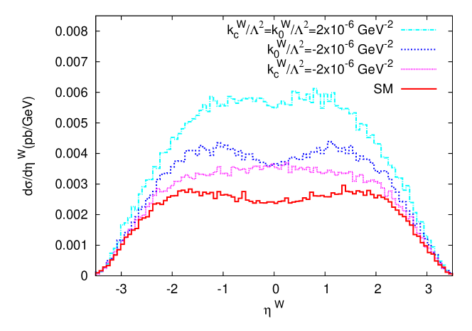
Figure 14: The rapidity distributions of $W^{+}$ boson in the final states using anomalous $\frac{k_{0}^{W}}{\Lambda^{2}}$ and $\frac{k_{c}^{W}}{\Lambda^{2}}$ couplings for the processes $e^{+}e^{-}\rightarrow e^{+}\gamma^{*}\gamma^{*}e^{-}\rightarrow e^{+}W^{+}W^{-}Ze^{-}$ at $\sqrt{s}=3$ TeV.

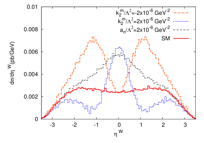
Figure 15: The rapidity distributions of $W^{+}$ boson in the final states using anomalous $\frac{k_{2}^{m}}{\Lambda^{2}}$ and $\frac{a_{n}}{\Lambda^{2}}$ couplings for the processes $e^{+}e^{-}\rightarrow e^{+}\gamma^{*}\gamma^{*}e^{-}\rightarrow e^{+}W^{+}W^{-}Ze^{-}$ at $\sqrt{s}=3$ TeV.

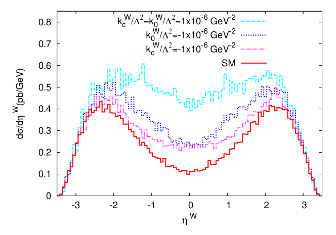
Figure 16: The rapidity distributions of $W^{+}$ boson in the final states using anomalous $\frac{k_{0}^{W}}{\Lambda^{2}}$ and $\frac{k_{c}^{W}}{\Lambda^{2}}$ couplings for the processes $\gamma\gamma\rightarrow W^{+}W^{-}Z$ at $\sqrt{s}=3$ TeV.

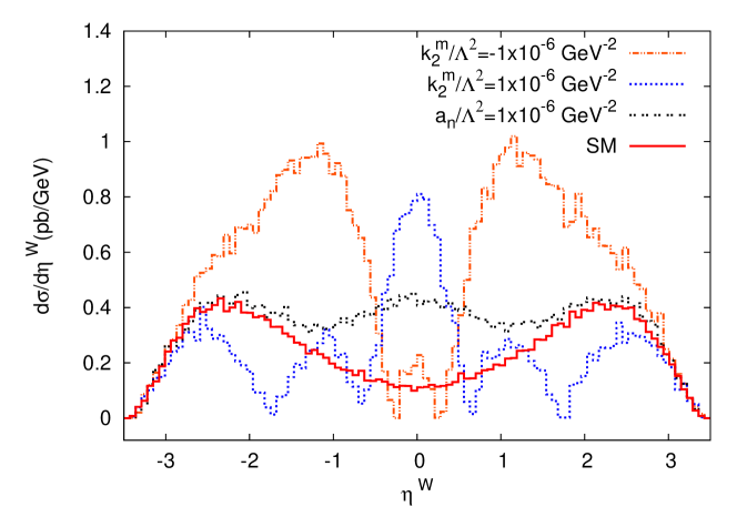
Figure 17: The rapidity distributions of $W^{+}$ boson in the final states using anomalous $\frac{k_{2}^{m}}{\Lambda^{2}}$ and $\frac{a_{n}}{\Lambda^{2}}$ couplings for the processes $\gamma\gamma\rightarrow W^{+}W^{-}Z$ at $\sqrt{s}=3$ TeV.

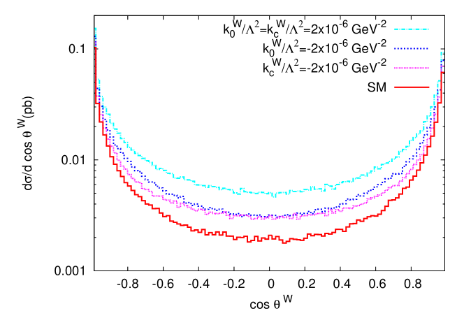
Figure 18: The angular distributions of $W^{+}$ boson in the final states using anomalous $\frac{k_{0}^{W}}{\Lambda^{2}}$ and $\frac{k_{c}^{W}}{\Lambda^{2}}$ couplings for the processes $e^{+}e^{-}\rightarrow e^{+}\gamma^{*}\gamma^{*}e^{-}\rightarrow e^{+}W^{+}W^{-}Ze^{-}$ at $\sqrt{s}=3$ TeV.

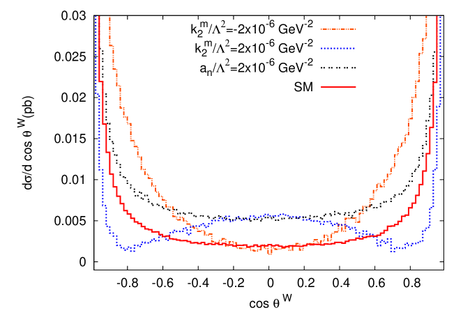
Figure 19: The angular distributions of $W^{+}$ boson in the final states using anomalous $\frac{k_{2}^{m}}{\Lambda^{2}}$ and $\frac{a_{n}}{\Lambda^{2}}$ couplings for the processes $e^{+}e^{-}\rightarrow e^{+}\gamma^{*}\gamma^{*}e^{-}\rightarrow e^{+}W^{+}W^{-}Ze^{-}$ at $\sqrt{s}=3$ TeV.

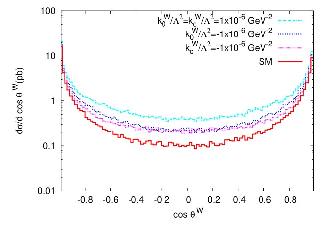
Figure 20: The angular distributions of $W^{+}$ boson in the final states using anomalous $\frac{k_{0}^{W}}{\Lambda^{2}}$ and $\frac{k_{c}^{W}}{\Lambda^{2}}$ couplings for the processes $\gamma\gamma\rightarrow W^{+}W^{-}Z$ at $\sqrt{s}=3$ TeV.

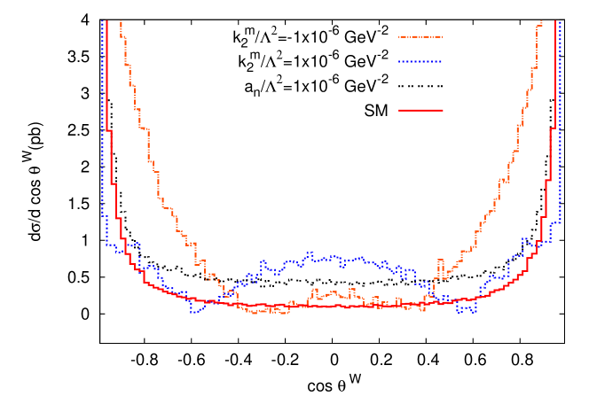
Figure 21: The angular distributions of $W^{+}$ boson in the final states using anomalous $\frac{k_{2}^{m}}{\Lambda^{2}}$ and $\frac{a_{n}}{\Lambda^{2}}$ couplings for the processes $\gamma\gamma\rightarrow W^{+}W^{-}Z$ at $\sqrt{s}=3$ TeV.

The kinematical distributions of final state particles can give further information about how we can separate among the different anomalous interactions. In this context, some distributions of the final state $W$ and $Z$ bosons are plotted for illustrative purposes using close to sensitivity of the anomalous couplings $\frac{k_{0}^{W}}{\Lambda^{2}}$, $\frac{k_{c}^{W}}{\Lambda^{2}}$, $\frac{k_{2}^{m}}{\Lambda^{2}}$ and $\frac{a_{n}}{\Lambda^{2}}$ in Figs. 10-21. We show the transverse momentum distributions of $Z$ boson in the final states using $\frac{k_{0}^{W}}{\Lambda^{2}}$, $\frac{k_{c}^{W}}{\Lambda^{2}}$ anomalous couplings in Fig. 10 and using $\frac{k_{2}^{m}}{\Lambda^{2}}$ and $\frac{a_{n}}{\Lambda^{2}}$ anomalous couplings in Fig. 11 for the processes $e^{+}e^{-}\rightarrow e^{+}\gamma^{*}\gamma^{*}e^{-}\rightarrow e^{+}W^{+}W^{-}Ze^{-}$ at $\sqrt{s}=3$ TeV. Similarly, the transverse momentum distributions for the $Z$ boson in the final states of the process $\gamma\gamma\rightarrow W^{+}W^{-}Z$ are given in Figs. 12-13. From this figures, we can separately observe the deviation of new physics induced by nonzero anomalous quartic CP-conserving and CP-violating couplings apart from SM background which is apparent at high $p_{T}$ region of the $Z$ bosons in the final states. The momentum dependence of the anomalous cross sections including the $WWZ\gamma$ vertices is higher than that of SM background cross section which causes the apparent deviation at high $p_{T}$ region.

We plot the rapidity distributions of the $W^{+}$ boson for two processes using the anomalous couplings $\frac{k_{0}^{W}}{\Lambda^{2}}$, $\frac{k_{c}^{W}}{\Lambda^{2}}$, $\frac{k_{2}^{m}}{\Lambda^{2}}$ and $\frac{a_{n}}{\Lambda^{2}}$ for $\sqrt{s}=3$ TeV in Figs. 14-17. Figs. 14-17 show that the rapidity distributions of the final state $W^{+}$ boson from the new physics signals and SM background are located generally in the range of $|\eta^{W}|<2.5$. Furthermore, we can easily discern the difference between positive and negative values of the coupling $\frac{k_{2}^{m}}{\Lambda^{2}}$. Especially, as can be seen from Fig. $15$, the anomalous interactions for $\frac{a_{n}}{\Lambda^{2}}$ coupling cause the production of more $W^{+}$ bosons in the central region.

In order to distinguish the different anomalous couplings with the SM, we illustrate the $cos\theta^{W}$ distributions of $W^{+}$ for two processes where $\theta^{W}$ is polar angle of $W^{+}$ with respect to the beam pipe. We show the $cos\theta^{W}$ distributions with the anomalous couplings $\frac{k_{0}^{W}}{\Lambda^{2}}$, $\frac{k_{c}^{W}}{\Lambda^{2}}$ and SM background in Fig. 18, using $\frac{k_{2}^{m}}{\Lambda^{2}}$ and $\frac{a_{n}}{\Lambda^{2}}$ couplings in Fig. 19 for $e^{+}e^{-}\rightarrow e^{+}\gamma^{*}\gamma^{*}e^{-}\rightarrow e^{+}W^{+}W^{-}Ze^{-}$ process at $\sqrt{s}=3$ TeV. Similarly, the $cos\theta^{W}$ distributions for the $\gamma\gamma\rightarrow W^{+}W^{-}Z$ process are given in Figs. 20-21. We can observe from these distributions that the contributions of negative and positive values of $\frac{k_{2}^{m}}{\Lambda^{2}}$ can easily be distinguished in Figs. 19 and 21.

In order to probe the sensitivity to the anomalous quartic $WWZ\gamma$ couplings, we use one and two-dimensional $\chi^{2}$ analysis:

$$\chi^{2}=\left(\frac{\sigma_{SM}-\sigma_{AN}(\frac{k_{0,c}^{W}}{\Lambda^{2}},\frac{k_{2}^{m}}{\Lambda^{2}},\frac{a_{n}}{\Lambda^{2}})}{\sigma_{SM}\delta_{stat}}\right)^{2}$$ (30)

where $\sigma_{AN}$ is the cross section including new physics effects, $\delta_{stat}=\frac{1}{\sqrt{N}}$ and $N$ is the number of SM events. The number of events for the processes $\gamma\gamma\rightarrow W^{+}W^{-}Z$ and $e^{+}e^{-}\rightarrow e^{+}\gamma^{*}\gamma^{*}e^{-}\rightarrow e^{+}W^{+}W^{-}Ze^{-}$ are obtained by $N=L_{int}\times\sigma_{SM}\times BR(Z\rightarrow\ell\bar{\ell})\times BR^{2}(W\rightarrow q\bar{q}^{\prime})$ where $L_{int}$ is the integrated luminosity. In addition, we assume that the the leptonic decay channel of $Z$ boson with branching ratio is $BR(Z\rightarrow\ell\bar{\ell})=0.067$ and the hadronic decay channel of $W$ boson with the branching ratio is $BR(W\rightarrow q\bar{q}^{\prime})=0.676$. In our calculations, one of the anomalous quartic couplings is assumed to deviate from their SM values (the others fixed to zero) at the one-dimensional $\chi^{2}$ analysis, while two anomalous quartic couplings ($\frac{k_{0,c}^{W}}{\Lambda^{2}}$) are assumed to deviate from their SM values at the two-dimensional $\chi^{2}$ analysis. In this case, we take into account $\chi^{2}$ value corresponding to the number of observable.

In Tables 1-4, we show $95\%$ C. L. sensitivities on the anomalous quartic couplings parameters $\frac{k_{0}^{W}}{\Lambda^{2}}$, $\frac{k_{c}^{W}}{\Lambda^{2}}$ , and $\frac{k_{2}^{m}}{\Lambda^{2}}$, $\frac{a_{n}}{\Lambda^{2}}$ for both two processes at $\sqrt{s}=0.5,1.5$ and $3$ TeV energies. As can be seen in Table 1, the process $\gamma\gamma\rightarrow W^{+}W^{-}Z$ improves the sensitivities of $\frac{k_{0}^{W}}{\Lambda^{2}}$ and $\frac{k_{c}^{W}}{\Lambda^{2}}$ by up to a factor of $10^{2}$ compared to the LHC sınır . The expected best sensitivities on $\frac{a_{n}}{\Lambda^{2}}$ in Table 2 are far beyond the sensitivities of the existing LEP. However, we compare our results with the sensitivities of Ref. mur , in which the best sensitivities on $\frac{k_{0}^{W}}{\Lambda^{2}}$, $\frac{k_{c}^{W}}{\Lambda^{2}}$, $\frac{k_{2}^{m}}{\Lambda^{2}}$ and $\frac{a_{n}}{\Lambda^{2}}$ couplings by examining the two processes $e^{+}e^{-}\rightarrow W^{-}W^{+}\gamma$ and $e^{+}e^{-}\rightarrow e^{+}\gamma^{*}e^{-}\rightarrow e^{+}W^{-}Z\nu_{e}$ at the 3 TeV CLIC are obtained. We observed that the sensitivities obtained on $\frac{k_{0}^{W}}{\Lambda^{2}}$ and $\frac{k_{c}^{W}}{\Lambda^{2}}$ are at the same order with those reported in the Ref. mur while sensitivities on $\frac{k_{2}^{m}}{\Lambda^{2}}$ and $\frac{a_{n}}{\Lambda^{2}}$ are 2 and 5 times better than the sensitivities calculated in Ref. mur , respectively. Our sensitivities on $\frac{k_{2}^{m}}{\Lambda^{2}}$ can set more stringent sensitive by two orders of magnitude with respect to the best sensitivity derived from $WZ\gamma$ production at the LHC with $\sqrt{s}=14$ TeV and the integrated luminosity of $L=200$ fb^-1 lhc1 .

The $\gamma^{*}\gamma^{*}$ collision of CLIC with $\sqrt{s}=3$ TeV and $L_{int}=590$ fb^-1 investigates the CP-conserving and CP-violating anomalous $WWZ\gamma$ coupling with a far better than the experiments sensitivities. One can see from Table 3 that the sensitivities on the anomalous couplings $\frac{k_{0}^{W}}{\Lambda^{2}}$ and $\frac{k_{c}^{W}}{\Lambda^{2}}$ are calculated as $[-1.09;\,1.09]\times 10^{-6}$ GeV^-2 and $[-1.54;\,1.54]\times 10^{-6}$ GeV^-2 which are an order of magnitude better than both $\frac{k_{0}^{W}}{\Lambda^{2}}$ and $\frac{k_{c}^{W}}{\Lambda^{2}}$ couplings. As shown in Table 4, the best sensitivities on $\frac{a_{n}}{\Lambda^{2}}$ coupling through the process $e^{+}e^{-}\rightarrow e^{+}\gamma^{*}\gamma^{*}e^{-}\rightarrow e^{+}W^{+}W^{-}Ze^{-}$ are obtained as $[-1.04;\,1.04]\times 10^{-6}$ GeV^-2 which are more stringent sensitivity by five orders of magnitude with respect to LEP results. Anomalous $\frac{k_{0}^{W}}{\Lambda^{2}}$ and $\frac{k_{c}^{W}}{\Lambda^{2}}$ couplings calculated with the help of the process $e^{+}e^{-}\rightarrow e^{+}\gamma^{*}\gamma^{*}e^{-}\rightarrow e^{+}W^{+}W^{-}Ze^{-}$ are less sensitive than the results of Ref. mur . On the other hand, our $\frac{k_{2}^{m}}{\Lambda^{2}}$ and $\frac{a_{n}}{\Lambda^{2}}$ couplings obtained from this process have similar sensitivities as Ref. mur .

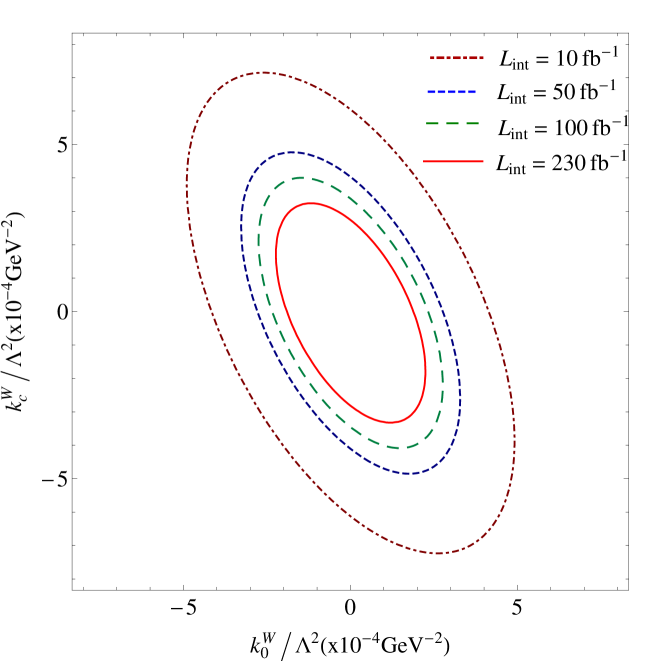
Figure 22: $95\%$ C.L. contours for anomalous $\frac{k_{0}^{W}}{\Lambda^{2}}$ and $\frac{k_{c}^{W}}{\Lambda^{2}}$ couplings for the process $e^{+}e^{-}\rightarrow e^{+}\gamma^{*}\gamma^{*}e^{-}\rightarrow e^{+}W^{+}W^{-}Ze^{-}$ at the CLIC with $\sqrt{s}=0.5$ TeV.

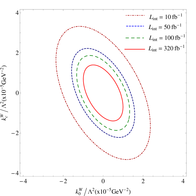
Figure 23: The same as Fig. 22 but for $\sqrt{s}=1.5$ TeV.

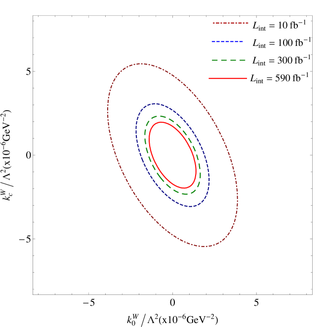
Figure 24: The same as Fig. 22 but for $\sqrt{s}=3$ TeV.

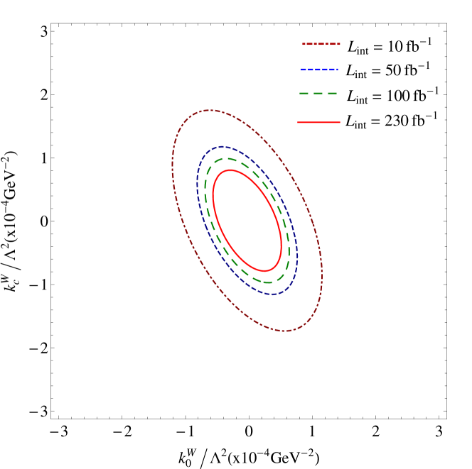
Figure 25: $95\%$ C.L. contours for anomalous $\frac{k_{0}^{W}}{\Lambda^{2}}$ and $\frac{k_{c}^{W}}{\Lambda^{2}}$ couplings for the process $\gamma\gamma\rightarrow W^{+}W^{-}Z$ at the CLIC with $\sqrt{s}=0.5$ TeV.

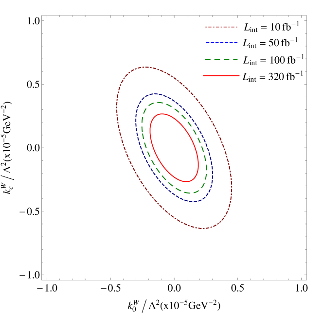
Figure 26: The same as Fig. 25 but for $\sqrt{s}=1.5$ TeV.

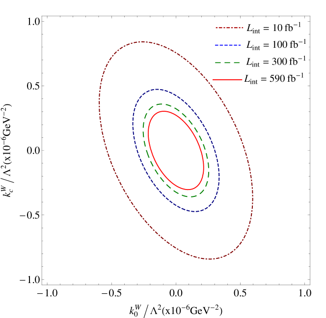
Figure 27: The same as Fig. 25 but for $\sqrt{s}=3$ TeV.

In Figs. 22-24, we present $95\%$ C.L. contours for anomalous $\frac{k_{0}^{W}}{\Lambda^{2}}$ and $\frac{k_{c}^{W}}{\Lambda^{2}}$ couplings for the process $e^{+}e^{-}\rightarrow e^{+}\gamma^{*}\gamma^{*}e^{-}\rightarrow e^{+}W^{+}W^{-}Ze^{-}$ at the CLIC for various integrated luminosities and center-of-mass energies. As we can see from Fig. 24, the best sensitivities on $\frac{k_{0}^{W}}{\Lambda^{2}}$ and $\frac{k_{c}^{W}}{\Lambda^{2}}$ through this process are [$-1.38\times 10^{-6}$, $1.38\times 10^{-6}$] and [$-1.96\times 10^{-6}$, $1.96\times 10^{-6}$], respectively for $L_{int}=590$ fb^-1 at the CLIC. Also, the same contours for the process $\gamma\gamma\rightarrow W^{+}W^{-}Z$ are given in Figs. 25-27. From two-parameter contours in Fig.27, the sensitivities for $\frac{k_{0}^{W}}{\Lambda^{2}}$ and $\frac{k_{c}^{W}}{\Lambda^{2}}$ are obtained as [$-2.15\times 10^{-6}$, $2.15\times 10^{-6}$ ] and [$-3.03\times 10^{-6}$, $3.03\times 10^{-6}$ ].

We can compare the obtained sensitivities on anomalous couplings by using statistical significance

$$SS=\frac{|\sigma_{tot}-\sigma_{SM}|}{\sqrt{\sigma_{SM}}}L_{int}$$ (31)

by assuming $\sqrt{s}=3$ TeV with the integrated luminosity of 590 fb^-1. Once again, we take into account leptonic decay channel of the final state $Z$ boson and hadronic decay channel of W boson for two processes. We obtain 3 (5) $\sigma$ observation sensitivities on the anomalous couplings from the $e^{+}e^{-}\rightarrow e^{+}\gamma^{*}\gamma^{*}e^{-}\rightarrow e^{+}W^{+}W^{-}Ze^{-}$ process;

$$-1.35(-1.74)\times 10^{-6}<\frac{k_{0}^{W}}{\Lambda^{2}}<1.35(1.74)\times 10^{-6}$$

$$-1.90(-2.45)\times 10^{-6}<\frac{k_{c}^{W}}{\Lambda^{2}}<1.90(2.45)\times 10^{-6}$$

$$-1.46(-1.89)\times 10^{-6}<\frac{k_{2}^{m}}{\Lambda^{2}}<1.46(1.89)\times 10^{-6}$$

$$-1.29(-1.66)\times 10^{-6}<\frac{a_{n}}{\Lambda^{2}}<1.29(1.66)\times 10^{-6}$$

and from the $\gamma\gamma\rightarrow W^{+}W^{-}Z$ process;

$$-2.14(-2.76)\times 10^{-7}<\frac{k_{0}^{W}}{\Lambda^{2}}<2.14(2.76)\times 10^{-7}$$

$$-3.02(-3.90)\times 10^{-7}<\frac{k_{c}^{W}}{\Lambda^{2}}<3.02(3.90)\times 10^{-7}$$

$$-2.33(-3.01)\times 10^{-7}<\frac{k_{2}^{m}}{\Lambda^{2}}<2.33(3.01)\times 10^{-7}$$

$$-2.09(-2.71)\times 10^{-7}<\frac{a_{n}}{\Lambda^{2}}<2.09(2.71)\times 10^{-7}.$$

The obtained sensitivities using signal significance at 5 $\sigma$ are approximately 1.5 times better than the best sensitivities obtained from $\chi^{2}$ analysis at 95% C.L..

III Conclusions

The linear $e^{-}e^{+}$ colliders will provide an important opportunity to probe $e\gamma$ and $\gamma\gamma$ collisions at high energies. In $e\gamma$ and $\gamma\gamma$ collisions, high energy real photons can be obtained by converting the incoming lepton beams into photon beams via the Compton backscattering mechanism. In addition, high-energy accelerated $e^{-}$ and $e^{+}$ beams at the linear colliders radiate quasi-real photons, and thus $e\gamma^{*}$ and $\gamma^{*}\gamma^{*}$ collisions are produced from the $e^{-}e^{+}$ process itself. Therefore, $e\gamma^{*}$ and $\gamma^{*}\gamma^{*}$ collisions at these colliders can occur spontaneously apart from $e\gamma$ and $\gamma\gamma$ collisions. In the literature, Refs. lhc1 ; lin2 only examined the sensitivities on $\frac{a_{n}}{\Lambda^{2}}$ couplings through the process $\gamma\gamma\rightarrow W^{+}W^{-}Z$ at future linear colliders. As stated in Ref. lin3 , the $\gamma\gamma$ collisions can examine the sensitivities on $\frac{a_{n}}{\Lambda^{2}}$ with a higher precision with respect to the $e\gamma$ and $e^{-}e^{+}$ collisions. For this reason, we compare our sensitivities with the results of Ref. mur . For $\frac{a_{n}}{\Lambda^{2}}$ couplings, $\gamma\gamma$ collisions at the 3 TeV CLIC with an integrated luminosity of $590$ fb^-1 enable us to improve the sensitivities by almost a factor of five with respect to sensitivities coming from $e^{-}e^{+}$ collisions. Also, our sensitivities show that $\gamma\gamma$ collisions provide anomalous $\frac{k_{2}^{m}}{\Lambda^{2}}$ couplings with a better than the $e^{-}e^{+}$ collisions. On the other hand, we can see that the sensitivities on $\frac{k_{0}^{W}}{\Lambda^{2}}$ and $\frac{k_{c}^{W}}{\Lambda^{2}}$ expected to be obtained for the future $\gamma\gamma$ colliders with $\sqrt{s}=3$ TeV are roughly 2 times worse than the sensitivities in Ref. mur . We find that the sensitivities obtained for four different $\frac{k_{0}^{W}}{\Lambda^{2}}$, $\frac{k_{c}^{W}}{\Lambda^{2}}$ and $\frac{k_{2}^{m}}{\Lambda^{2}}$ and $\frac{a_{n}}{\Lambda^{2}}$ couplings from the process $\gamma\gamma\rightarrow W^{+}W^{-}Z$ are approximately an order of magnitude more restrictive with respect to the main process $e^{+}e^{-}\rightarrow e^{+}\gamma^{*}\gamma^{*}e^{-}\rightarrow e^{+}W^{+}W^{-}Ze^{-}$ which is obtained by integrating the cross section for the subprocess $\gamma^{*}\gamma^{*}\rightarrow W^{+}W^{-}Z$ over the effective photon luminosity. The process $\gamma\gamma(\gamma^{*}\gamma^{*})\rightarrow W^{+}W^{-}Z$ includes only interactions between the gauge bosons, causing more apparent possible deviations from the expected value of SM lin3 . Therefore, in this paper, we analyze the CP-conserving parameters $\frac{k_{0}^{W}}{\Lambda^{2}}$, $\frac{k_{c}^{W}}{\Lambda^{2}}$ and $\frac{k_{2}^{m}}{\Lambda^{2}}$ and CP-violating parameter $\frac{a_{n}}{\Lambda^{2}}$ on the anomalous quartic $WWZ\gamma$ gauge couplings through the processes $\gamma\gamma\rightarrow W^{+}W^{-}Z$ obtained by laser-backscattering distributions and $e^{+}e^{-}\rightarrow e^{+}\gamma^{*}\gamma^{*}e^{-}\rightarrow e^{+}W^{+}W^{-}Ze^{-}$ derived by EPA distributions at the CLIC. The $\gamma\gamma$ collisions seem to be the best place to test $\frac{k_{2}^{m}}{\Lambda^{2}}$ and $\frac{a_{n}}{\Lambda^{2}}$ which are the anomalous quartic couplings involving photons. Therefore, the CLIC as photon-photon collider provides an ideal platform to examine anomalous quartic $WWZ\gamma$ gauge couplings at high energies.

*

Appendix A The anomalous vertex functions derived from CP-violating and CP-conserving effective Lagrangians

The anomalous $W^{+}(p_{1}^{\alpha})W^{-}(p_{2}^{\beta})Z(k_{2}^{\nu})\gamma(k_{1}^{\mu})$ vertex function obtained from CP-violating effective $\textit{L}_{n}$ Lagrangian is given below

$$i\frac{\pi\alpha}{4\textmd{cos}\,\,\theta_{W}\Lambda^{2}}a_{n}[g_{\alpha\nu}[g_{\beta\mu}\,k_{1}.(k_{2}-p_{1})-k_{1\beta}.(k_{2}-p_{1})_{\mu}]$$

$$-g_{\beta\nu}[g_{\alpha\mu}\,k_{1}.(k_{2}-p_{2})-k_{1\alpha}.(k_{2}-p_{2})_{\mu}]$$

$$+g_{\alpha\beta}[g_{\nu\mu}k_{1}.(p_{1}-p_{2})-k_{1\nu}.(p_{1}-p_{2})_{\mu}]$$

$$-k_{2\alpha}(g_{\beta\mu}k_{1\nu}-g_{\nu\mu}k_{1\beta})+k_{2\beta}(g_{\alpha\mu}k_{1\nu}-g_{\nu\mu}k_{1\alpha})$$

$$-p_{2\nu}(g_{\alpha\mu}k_{1\beta}-g_{\beta\mu}k_{1\alpha})+p_{1\nu}(g_{\beta\mu}k_{1\alpha}-g_{\alpha\mu}k_{1\beta})$$

$$+p_{1\beta}(g_{\nu\mu}k_{1\alpha}-g_{\alpha\mu}k_{1\nu})+p_{2\alpha}(g_{\nu\mu}k_{1\beta}-g_{\beta\mu}k_{1\nu})].$$ (32)

The anomalous $W^{+}(p_{1}^{\alpha})W^{-}(p_{2}^{\beta})Z(k_{2}^{\nu})\gamma(k_{1}^{\mu})$ vertex functions obtained from CP-conserving effective $\textit{W}_{0}^{Z},\textit{W}_{c}^{Z},\textit{W}_{1}^{Z},\textit{W}_{2}^{Z}$ and $\textit{W}_{3}^{Z}$ can be written as follows, respectively

$$2ie^{2}g^{2}g_{\alpha\beta}[g_{\mu\nu}(k_{1}.k_{2})-k_{1\nu}k_{2\mu}],$$ (33)

$$i\frac{e^{2}g^{2}}{2}[(g_{\mu\alpha}g_{\nu\beta}+g_{\nu\alpha}g_{\mu\beta})(k_{1}.k_{2})+g_{\mu\nu}(k_{2\beta}k_{1\alpha}+k_{1\beta}k_{2\alpha})$$

$$-k_{2\mu}k_{1\alpha}g_{\nu\beta}-k_{2\beta}k_{1\nu}g_{\mu\alpha}-k_{2\alpha}k_{1\nu}g_{\mu\beta}-k_{2\mu}k_{1\beta}g_{\nu\alpha}],$$ (34)

$$ieg_{z}g^{2}((g_{\mu\alpha}k_{1}.p_{1}-p_{1\mu}k_{1\alpha})g_{\nu\beta}+(g_{\mu\beta}k_{1}.p_{2}-p_{2\mu}k_{1\beta})g_{\nu\alpha})$$ (35)

$$i\frac{eg_{z}g^{2}}{2}((k_{1}.p_{1}+k_{1}.p_{2})g_{\mu\nu}g_{\alpha\beta}-(k_{1\alpha}p_{1\beta}+k_{1\beta}p_{2\alpha})g_{\mu\nu}$$

$$-(p_{1\mu}+p_{2\mu})k_{1\nu}g_{\alpha\beta}+(p_{1\beta}g_{\mu\alpha}+p_{2\alpha}g_{\mu\beta})k_{1\nu}),$$ (36)

$$i\frac{eg_{z}g^{2}}{2}(k_{1}.p_{1}g_{\mu\beta}g_{\nu\alpha}+k_{1}.p_{2}g_{\mu\alpha}g_{\nu\beta}+(p_{1\nu}-p_{2\nu})k_{1\beta}g_{\mu\alpha}$$

$$-(p_{1\nu}-p_{2\nu})k_{1\alpha}g_{\mu\beta}-p_{1\mu}k_{1\beta}g_{\nu\alpha}-p_{2\mu}k_{1\alpha}g_{\nu\beta}).$$ (37)

Figure 1: Schematic diagram for the process $e^{+}e^{-}\rightarrow e^{+}\gamma^{*}\gamma^{*}e^{-}\rightarrow e^{+}W^{+}W^{-}Ze^{-}$ at the CLIC.

Figure 6: The total cross sections as function of anomalous $\frac{k_{0}^{W}}{\Lambda^{2}}$, $\frac{k_{c}^{W}}{\Lambda^{2}}$ and $\frac{k_{2}^{m}}{\Lambda^{2}}$ couplings for the process $\gamma\gamma\rightarrow W^{+}W^{-}Z$ at the CLIC with $\sqrt{s}=0.5$ TeV.

Figure 9: The total cross sections as function of anomalous $\frac{a_{n}}{\Lambda^{2}}$ coupling for the process $\gamma\gamma\rightarrow W^{+}W^{-}Z$ at the CLIC with $\sqrt{s}=0.5,1.5$ and $3$ TeV.

Table 1: The sensitivities of the anomalous $\frac{k_{0}^{W}}{\Lambda^{2}}$ and $\frac{k_{c}^{W}}{\Lambda^{2}}$ couplings through the process $\gamma\gamma\rightarrow W^{+}W^{-}Z$ at the CLIC with $\sqrt{s}=0.5,1.5$ and $3$ TeV for various integrated luminosities.

$\sqrt{s}$ (TeV)	$L_{int}$(fb-1)	$\frac{k_{0}^{W}}{\Lambda^{2}}$(GeV-2)	$\frac{k_{c}^{W}}{\Lambda^{2}}$ (GeV-2)
$0.5$	$10$	$[-9.39;8.91]\times 10^{-5}$	$[-1.36;\,1.34]\times 10^{-4}$
$0.5$	$50$	$[-6.36;\,5.88]\times 10^{-5}$	$[-9.14;\,8.93]\times 10^{-5}$
$0.5$	$100$	$[-5.39;\,4.91]\times 10^{-5}$	$[-7.69;\,7.49]\times 10^{-5}$
$0.5$	$230$	$[-4.42;\,3.94]\times 10^{-5}$	$[-6.27;\,6.06]\times 10^{-5}$
$1.5$	$10$	$[-3.50;\,3.50]\times 10^{-6}$	$[-4.92;\,4.92]\times 10^{-6}$
$1.5$	$50$	$[-2.34;\,2.34]\times 10^{-6}$	$[-3.29;\,3.29]\times 10^{-6}$
$1.5$	$100$	$[-1.97;\,1.97]\times 10^{-6}$	$[-2.77;\,2.77]\times 10^{-6}$
$1.5$	$320$	$[-1.47;\,1.47]\times 10^{-6}$	$[-2.07;\,2.07]\times 10^{-6}$
$3$	$10$	$[-4.80;\,4.80]\times 10^{-7}$	$[-6.77;\,6.77]\times 10^{-7}$
$3$	$100$	$[-2.69;\,2.69]\times 10^{-7}$	$[-3.81;\,3.81]\times 10^{-7}$
$3$	$300$	$[-2.05;\,2.05]\times 10^{-7}$	$[-2.89;\,2.89]\times 10^{-7}$
$3$	$590$	$[-1.73;\,1.73]\times 10^{-7}$	$[-2.44;\,2.44]\times 10^{-7}$

Table 2: The sensitivities of the anomalous $\frac{k_{2}^{m}}{\Lambda^{2}}$ and $\frac{a_{n}}{\Lambda^{2}}$ couplings through the process $\gamma\gamma\rightarrow W^{+}W^{-}Z$ at the CLIC with $\sqrt{s}=0.5,1.5$ and $3$ TeV for various integrated luminosities.

$\sqrt{s}$ (TeV)	$L_{int}$(fb-1)	$\frac{k_{2}^{m}}{\Lambda^{2}}$(GeV-2)	$\frac{a_{n}}{\Lambda^{2}}$ (GeV-2)
$0.5$	$10$	$[-2.17;2.09]\times 10^{-4}$	$[-3.59;\,3.59]\times 10^{-4}$
$0.5$	$50$	$[-1.47;\,1.39]\times 10^{-4}$	$[-2.40;\,2.40]\times 10^{-4}$
$0.5$	$100$	$[-1.24;\,1.16]\times 10^{-4}$	$[-2.02;\,2.02]\times 10^{-4}$
$0.5$	$230$	$[-1.01;\,0.94]\times 10^{-5}$	$[-1.64;\,1.64]\times 10^{-4}$
$1.5$	$10$	$[-5.22;\,5.21]\times 10^{-6}$	$[-6.04;\,6.04]\times 10^{-6}$
$1.5$	$50$	$[-3.49;\,3.49]\times 10^{-6}$	$[-4.04;\,4.04]\times 10^{-6}$
$1.5$	$100$	$[-2.93;\,2.93]\times 10^{-6}$	$[-3.39;\,339]\times 10^{-6}$
$1.5$	$320$	$[-2.19;\,2.19]\times 10^{-6}$	$[-2.54;\,2.54]\times 10^{-6}$
$3$	$10$	$[-5.23;\,5.23]\times 10^{-7}$	$[-4.70;\,4.70]\times 10^{-7}$
$3$	$100$	$[-2.94;\,2.94]\times 10^{-7}$	$[-2.64;\,2.64]\times 10^{-7}$
$3$	$300$	$[-2.23;\,2.23]\times 10^{-7}$	$[-2.01;\,2.01]\times 10^{-7}$
$3$	$590$	$[-1.89;\,1.89]\times 10^{-7}$	$[-1.74;\,1.74]\times 10^{-7}$

Table 3: The sensitivities of the anomalous $\frac{k_{0}^{W}}{\Lambda^{2}}$ and $\frac{k_{c}^{W}}{\Lambda^{2}}$ couplings through the process $e^{+}e^{-}\rightarrow e^{+}\gamma^{*}\gamma^{*}e^{-}\rightarrow e^{+}W^{+}W^{-}Ze^{-}$ at the CLIC with $\sqrt{s}=1.5$ and $3$ TeV for various integrated luminosities.

$\sqrt{s}$ (TeV)	$L_{int}$(fb-1)	$\frac{k_{0}^{W}}{\Lambda^{2}}$(GeV-2)	$\frac{k_{c}^{W}}{\Lambda^{2}}$ (GeV-2)
$0.5$	$10$	$[-3.72;\,3.71]\times 10^{-4}$	$[-5.48;\,5.41]\times 10^{-4}$
$0.5$	$50$	$[-2.49;\,2.48]\times 10^{-4}$	$[-3.68;\,3.61]\times 10^{-4}$
$0.5$	$100$	$[-2.09;\,2.08]\times 10^{-4}$	$[-3.10;\,3.02]\times 10^{-4}$
$0.5$	$230$	$[-1.70;\,1.69]\times 10^{-4}$	$[-2.52;\,2.45]\times 10^{-4}$
$1.5$	$10$	$[-1.83;\,1.83]\times 10^{-5}$	$[-2.58;\,2.58]\times 10^{-5}$
$1.5$	$50$	$[-1.23;\,1.23]\times 10^{-5}$	$[-1.72;\,1.72]\times 10^{-5}$
$1.5$	$100$	$[-1.03;\,1.03]\times 10^{-5}$	$[-1.45;\,1.45]\times 10^{-5}$
$1.5$	$320$	$[-7.71;\,7.71]\times 10^{-6}$	$[-1.08;\,1.08]\times 10^{-5}$
$3$	$10$	$[-3.03;\,3.03]\times 10^{-6}$	$[-4.27;\,4.27]\times 10^{-6}$
$3$	$100$	$[-1.70;\,1.70]\times 10^{-6}$	$[-2.40;\,2.40]\times 10^{-6}$
$3$	$300$	$[-1.29;\,1.29]\times 10^{-6}$	$[-1.82;\,1.82]\times 10^{-6}$
$3$	$590$	$[-1.09;\,1.09]\times 10^{-6}$	$[-1.54;\,1.54]\times 10^{-6}$

Table 4: The sensitivities of the anomalous $\frac{k_{2}^{m}}{\Lambda^{2}}$ and $\frac{a_{n}}{\Lambda^{2}}$ couplings through the process $e^{+}e^{-}\rightarrow e^{+}\gamma^{*}\gamma^{*}e^{-}\rightarrow e^{+}W^{+}W^{-}Ze^{-}$ at the CLIC with $\sqrt{s}=1.5$ and $3$ TeV for various integrated luminosities.

$\sqrt{s}$ (TeV)	$L_{int}$(fb-1)	$\frac{k_{2}^{m}}{\Lambda^{2}}$(GeV-2)	$\frac{a_{n}}{\Lambda^{2}}$ (GeV-2)
$0.5$	$10$	$[-8.46;\,8.20]\times 10^{-4}$	$[-1.35;\,1.35]\times 10^{-4}$
$0.5$	$50$	$[-5.70;\,5.44]\times 10^{-4}$	$[-9.02;\,9.02]\times 10^{-5}$
$0.5$	$100$	$[-4.81;\,4.55]\times 10^{-4}$	$[-7.56;\,7.56]\times 10^{-5}$
$0.5$	$230$	$[-3.93;\,3.67]\times 10^{-4}$	$[-6.15;\,6.15]\times 10^{-5}$
$1.5$	$10$	$[-2.72;\,2.72]\times 10^{-5}$	$[-3.10;\,3.10]\times 10^{-5}$
$1.5$	$50$	$[-1.82;\,1.82]\times 10^{-5}$	$[-2.07;\,2.07]\times 10^{-5}$
$1.5$	$100$	$[-1.53;\,1.53]\times 10^{-5}$	$[-1.74;\,1.74]\times 10^{-5}$
$1.5$	$320$	$[-1.14;\,1.14]\times 10^{-5}$	$[-1.30;\,1.30]\times 10^{-5}$
$3$	$10$	$[-3.28;\,3.28]\times 10^{-6}$	$[-2.89;\,2.89]\times 10^{-6}$
$3$	$100$	$[-1.84;\,1.84]\times 10^{-6}$	$[-1.62;\,1.62]\times 10^{-6}$
$3$	$300$	$[-1.40;\,1.40]\times 10^{-6}$	$[-1.24;\,1.24]\times 10^{-6}$
$3$	$590$	$[-1.18;\,1.18]\times 10^{-6}$	$[-1.04;\,1.04]\times 10^{-6}$

References

• (1) O. J. P. Eboli, M. C. Gonzalez-Garcia and S. F. Novaes, Nucl. Phys. B 411, 381 (1994).
• (2) O. J. P. Eboli, M.C. Gonzalez-Garcia and S. M. Lietti, Phys. Rev. D 69, 095005 (2004).
• (3) G. Belanger, F. Boudjema, Y. Kurihara, D. Perret-Gallix and A. Semenov, Eur. Phys. J. C 13, 283-293 (2000).
• (4) P. Achard $et\>al.$, L3 collaboration, Phys. Lett. B 527, 29 (2002).
• (5) J. Abdallah $et\>al.$, DELPHI collaboration, Eur. Phys. J. C 31, 139 (2003).
• (6) G. Abbiendi $et\>al.$, OPAL collaboration, Phys. Lett. B 580, 17 (2004).
• (7) S. Chatrchyan $et\>al.$, CMS collaboration, arXiv:1404.4619 [hep-ex].
• (8) G. Abu Leil and W. J. Stirling, J. Phys. G 21, 517 (1995).
• (9) W. J. Stirling and A. Werthenbach, Eur. Phys. J. C 14, 103 (2000).
• (10) A. Denner $et\>al.$, Eur. Phys. J. C 20, 201 (2001).
• (11) G. Montagna $et\>al.$, Phys. Lett. B 515, 197 (2001).
• (12) M. Beyer $et\>al.$, Eur. Phys. J. C 48, 353 (2006).
• (13) M. KΓΆksal and A. Senol, arXiv:1406.2496.
• (14) I. Sahin, J. Phys. G: Nucl. Part. Phys. 35, 035006 (2008).
• (15) O. J. P. Eboli, M. B. Magro, P. G. Mercadante and S. F. Novaes, Phys. Rev. D 52, 15 (1995).
• (16) I. Sahin, J. Phys. G: Nucl. Part. Phys. 36, 075007 (2009).
• (17) Ke Ye, Daneng Yang and Qiang Li, Phys. Rev. D 88, 015023 (2013).
• (18) A. Senol and M. KΓΆksal, Phys. Lett. B 742, 143 (2015) [arXiv:1410.3648 [hep-ph]].
• (19) T.Β Pierzchala and K.Β Piotrzkowski, Nucl.Β Phys.Β Proc.Β Suppl.Β 179, 257 (2008) [arXiv:0807.1121 [hep-ph]].
• (20) E.Β Chapon, C.Β Royon and O.Β Kepka, Phys.Β Rev.Β D 81, 074003 (2010) [arXiv:0912.5161 [hep-ph]].
• (21) J.Β de Favereau de Jeneret, V.Β Lemaitre, Y.Β Liu, S.Β Ovyn, T.Β Pierzchala, K.Β Piotrzkowski, X.Β Rouby and N.Β Schul et al., arXiv:0908.2020 [hep-ph].
• (22) R.Β S.Β Gupta, Phys.Β Rev.Β D 85, 014006 (2012) [arXiv:1111.3354 [hep-ph]].
• (23) D. Dannheim $et\>al.$, CLIC $e^{+}e^{-}$ Linear Collider Studies, arXiv:1305.5766v1.
• (24) I. F. Ginzburg, G. L. Kotkin, V. G. Serbo and V. I. Telnov, Nucl. Instr. and Meth. 205, 47 (1983).
• (25) I. F. Ginzburg, G. L. Kotkin, S. L. Panfil, V. G. Serbo and V. I. Telnov, Nucl. Instr. and Meth. 219, 5 (1984).
• (26) S.Β J.Β Brodsky, T.Β Kinoshita and H.Β Terazawa, Phys. Rev. D 4, 1532 (1971).
• (27) H.Β Terazawa, Rev. Mod. Phys. 45, 615 (1973).
• (28) V.M. Budnev, I.F. Ginzburg, G.V. Meledin and V.G. Serbo, Phys. Rept. 15, 181 (1974).
• (29) K. Piotrzkowski, Phys. Rev. D 63, 071502 (2001).
• (30) G. Baur et al., Phys. Rep. 364, 359 (2002).
• (31) J. Abdallah $et\>al.$, DELPHI Collaboration, Eur. Phys. J. C 35, 159 (2004).
• (32) A. Abulencia $et\>al.$, CDF Collaboration, Phys. Rev. Lett. 98, 112001 (2007).
• (33) T. Aaltonen $et\>al.$, CDF Collaboration, Phys. Rev. Lett. 102, 222002 (2009).
• (34) T. Aaltonen $et\>al.$, CDF Collaboration, Phys. Rev. Lett. 102, 242001 (2009).
• (35) S. Chatrchyan $et\>al.$, CMS Collaboration, JHEP 1201, 052 (2012).
• (36) S. Chatrchyan et al:, CMS Collaboration, JHEP 1211, 080 (2012).
• (37) S. Atag and A. Billur, JHEP 11, 060 (2010).
• (38) S. Atag, S. C. Δ°nan and Δ°. Sahin, Phys. Rev. D 80, 075009 (2009).
• (39) Δ°. Sahin and S. C. Δ°nan, JHEP 09, 069 (2009).
• (40) S. C. Δ°nan, Phys. Rev. D 81, 115002 (2010).
• (41) Δ°. Sahin and M. KΓΆksal, JHEP 11, 100 (2011).
• (42) M. KΓΆksal and S. C. Δ°nan, Adv.High Energy Phys. 2014, 935840 (2014).
• (43) M. KΓΆksal and S. C. Δ°nan, Adv.High Energy Phys. 2014, 315826 (2014).
• (44) A. A. Billur and M. KΓΆksal, Phys. Rev. D 89, 037301 (2014).
• (45) A. Senol, Phys. Rev. D 87, 073003 (2013).
• (46) A. Senol, Int.Β J.Β Mod.Β Phys.Β A 29, 1450148 (2014).
• (47) Δ°. Şahin $et\>al.$, Phys.Rev. D 88, 095016 (2013).
• (48) S. C. Δ°nan and A. Billur, Phys. Rev. D 84, 095002 (2011).
• (49) Δ°. Sahin, Phys. Rev. D 85, 033002 (2012).
• (50) Δ°. Sahin and B. Sahin, Phys. Rev. D 86, 115001 (2012).
• (51) B. Sahin and A. A. Billur, Phys. Rev. D 86, 074026 (2012).
• (52) A. A. Billur, Europhys. Lett. 101, 21001 (2013).
• (53) M. Tasevsky, Nucl. Phys. Proc. Suppl. 179-180 187-195 (2008).
• (54) M. Tasevsky, arXiv:0910.5205.
• (55) H. Sun, Nucl. Phys. B 886, 691 (2014).
• (56) H. Sun and Chong-Xing Yue, Eur.Phys.J. C 74, 2823 (2014).
• (57) H. Sun, Phys.Rev. D 90, 035018 (2014).
• (58) H. Sun, Ya-Jin Zhou and Hong-Sheng Hou, arXiv:1408.1218.
• (59) Δ°. Sahin $et\>al.$, arXiv:1409.1796
• (60) M. KΓΆksal, Int. J. Mod. Phys. A 29, 1450138 (2014).
• (61) M. KΓΆksal, Mod. Phys. Lett. A 29, 1450184 (2014).
• (62) M. KΓΆksal, arXiv:1402.3773.
• (63) A. A. Billur and M. KΓΆksal, Phys.Rev. D 89, 3 037301 (2014).
• (64) J. E. Cieza Montalvo, G.H. Ramrez Ulloa, M.D. Tonasse, Eur. Phys. J. C 72, 2210 (2012).
• (65) A. Belyaev, N. D. Christensen and A. Pukhov, Comput. Phys. Commun. 184, 1729 (2013) [arXiv:1207.6082 [hep-ph]].
Refer to caption