Accurate multiple time step in biased molecular simulations

Abstract

Many recently introduced enhanced sampling techniques are based on biasing coarse descriptors (collective variables) of a molecular system on the fly. Sometimes the calculation of such collective variables is expensive and becomes a bottleneck in molecular dynamics simulations. An algorithm to treat smooth biasing forces within a multiple time step framework is here discussed. The implementation is simple and allows a speed up when expensive collective variables are employed. The gain can be substantial when using massively parallel or GPU-based molecular dynamics software. Moreover, a theoretical framework to assess the sampling accuracy is introduced, which can be used to assess the choice of the integration time step in both single and multiple time step biased simulations.

I Introduction

Molecular simulations allow the dynamics of a system to be followed at atomistic resolution and thus can be used as virtual microscopes to investigate chemical reactions and conformational transitions in molecular systems Allen and Tildesley (1987); Frenkel and Smit (2002); Tuckerman (2010). The time scale that can be simulated with current computers and algorithms is on the order of a microsecond for a system of a few tens of thousands of atoms modeled with a typical atomistic empirical force field. Even though recently developed ad hoc hardware allowed for a sudden jump in this scale Dror et al. (2011), many relevant processes are still out of range for atomistic molecular dynamics (MD). A lot of effort has been made in the last decades to tackle or, at least, to alleviate this issue by means of modified algorithms known as enhanced sampling techniques. Among these, a class of methods is based on the idea of biasing a few, carefully selected collective degrees of freedom, known as collective variables (CVs) Torrie and Valleau (1977); Darve and Pohorille (2001); Laio and Parrinello (2002); Maragliano and Vanden-Eijnden (2006); Marsili et al. (2006); Barducci et al. (2008); Abrams and Tuckerman (2008); Laio and Gervasio (2008); Barducci et al. (2011); Abrams and Bussi (2014); Dellago and Hummer (2014). Biased enhanced-sampling simulations require these descriptors to be computed on the fly at every simulation time step. The cost of computing the CVs can in principle slow down the calculation. This is particularly true for expensive CVs, such as Steinhardt order parameters Steinhardt et al. (1983); Trudu et al. (2006), path CVs Branduardi et al. (2007), template-based CVs Pietrucci and Laio (2009), property maps Spiwok and Králová (2011), social permutation-invariant coordinates Pietrucci and Andreoni (2011), sketch maps Tribello et al. (2012) and Debye-Hückel energy Do et al. (2013), just to mention a few. The calculation of the CVs and of the resulting biasing forces can be done in dedicated routines of MD software or can be implemented in external plugins Bonomi et al. (2009); Fiorin et al. (2013); Tribello et al. (2014). It is very difficult to optimize the calculation of the CVs for several reasons. First, they sometime involve long-range exchange of information that makes them difficult to be compatible with domain-decomposition algorithms. Second, because their definition is highly system dependent, routines implementing these schemes should be flexible, thus paying an unavoidable price in terms of efficiency. On the opposite side, the calculation of physical force fields is becoming faster and faster thanks to the use of massively parallel and optimized software Plimpton (1995); Van Der Spoel et al. (2005); Phillips et al. (2005) and hardware Dror et al. (2011). The overall consequence of this trend is that the calculation of CVs can be expected to become a relevant bottleneck in enhanced sampling simulations, particularly in the context of massively parallel or GPU-accelerated MD.

We here introduce a scheme based on multiple time step integration (MTS) in its reference system propagator algorithm (RESPA) formulation Tuckerman et al. (1992); Sexton and Weingarten (1992). More precisely, MTS is used here to split the integration of biasing forces and physical forces. The underlying principle is that often the former have a smoother dependence on atomic positions, thus change at a lower rate and can be integrated with a larger time step. This splitting allows for a substantial increase in the computational efficiency of biased sampling methods. Furthermore, we introduce a theoretical framework so as to assess the unavoidable time-step discretization errors. This is done by extending the concept of effective energy Bussi et al. (2007); Bussi and Parrinello (2007) so as to take into account the effect of biasing forces separately. This scheme allows artifacts that could be hidden when observing total-energy conservation to be highlighted. In the Method Section we introduce the methodology, first reviewing the MTS integration then introducing the scheme to assess sampling accuracy. We then present numerical tests of our algorithm on a one-dimensional model, on alanine dipeptide and on a large protein/RNA complex, using CVs of increasing complexity. In the latter case we show that the use of MTS can greatly improve the performance without introducing significant errors.

II Methods

II.1 Multiple time step

We consider here a system of $N_{at}$ atoms evolving accordingly to biased Hamilton equations in the form:

$$\dot{\mathbf{q}}_{i} =\frac{\mathbf{p}_{i}}{m_{i}}$$

$$\dot{\mathbf{p}}_{i} =-\frac{\partial U}{\partial\mathbf{q}_{i}}-\frac{\partial V}{\partial\mathbf{q}_{i}}=-\frac{\partial U}{\partial\mathbf{q}_{i}}-\sum_{\alpha=1}^{N_{cv}}\frac{\partial V}{\partial s_{\alpha}}\frac{\partial s_{\alpha}}{\partial\mathbf{q}_{i}}\,.$$

Here $\mathbf{q}_{i}$, $\mathbf{p}_{i}$, and $m_{i}$ are respectively coordinates, momenta, and mass of $i$-th atom; $U(q)$ is the physical potential, typically obtained evaluating an empirical force field (see, e.g., Ref. Cornell et al. (1995)); $V(s)$ is a biasing potential, which depends on the atomic positions only through $N_{cv}$ collective variables $s_{\alpha}(q)$.

The choice of the time step $\Delta t$ for the integration of the equations of motion is dictated by the fastest frequencies of the system, which depend on the atomic masses and on the functional form of $U$. In reversible MTS integration forces are typically split in a fast-changing part and slow-changing part, so that different integration time steps can be used for the two parts Tuckerman et al. (1992); Sexton and Weingarten (1992). Ideally, the slow-changing part is the most computationally expensive one.

We remark here that CVs are often smoother functions of atomic coordinates than the stiffest force-field terms. As an example, CVs used for isomerization processes such as torsional angles are typically slower when compared with bond fluctuations. Biasing forces are thus good candidates for the time-reversible MTS scheme itemized below:

1. Integrate momenta according to biasing force $-\frac{\partial V}{\partial\mathbf{q}_{i}}$ for a single time step of length $\frac{n\Delta t}{2}$.

2. Integrate momenta and positions according to the physical forces $-\frac{\partial U}{\partial\mathbf{q}_{i}}$ for $n$ times, with time step $\Delta t$.

3. Integrate momenta according to biasing force $-\frac{\partial V}{\partial\mathbf{q}_{i}}$ for a single time step of length $\frac{n\Delta t}{2}$.

Here $\Delta t$ is the inner time step and $n$ is the order of the MTS scheme, so that biasing forces and, as a consequence, CVs are only evaluated with a time step $n\Delta t$. This algorithm can be straightforwardly integrated in existing codes. Indeed, it is sufficient to apply the biasing forces every $n$ steps scaling them by a factor $n$ so as to take correctly into account the transferred momentum. In the intermediate $(n-1)$ steps, CVs do not need to be computed. The algorithm is by construction symplectic and reversible, as long as the underlying integrator for the Hamilton equations is symplectic and reversible.

We note that a too large outer time step $n\Delta t$ can lead to the well-known occurrence of resonances Biesiadecki and Skeel (1993) and thus to significant systematic errors. Several possible solutions have been recently proposed to tackle this issue.Morrone et al. (2011); Leimkuhler et al. (2013) These recent improvements could be easily coupled with the presented algorithm and might decrease the systematic errors. We also observe that so-called multigrators Lippert et al. (2013) do not suffer from resonances because they are based on splitting in two equations of motion both having the same stationary distribution and thus can be used with arbitrarily large $n$. Such an approach is not suitable in the context discussed here. However, we notice that in typical situations even small values of $n$ are already enough to largely decrease the effective computational cost of CV calculation. Finally, we observe that MTS has been also employed in Ref. Abrams and Tuckerman (2008) with a different purpose, i.e. to allow for a large time step for the physical force-field to be combined with a short time step for the integration of the CVs.

II.2 Assessment of sampling error

In order to provide results free from systematic errors, enhanced sampling methods should be paired with integration of the equations of motion able to correctly sample the target statistical ensemble, which is typically the isothermal or the isobaric one. In general, the errors in the stationary distribution depends in a non-trivial way on the integration algorithm and on the details of the underlying potential (see, e.g., Ref. Leimkuhler and Matthews (2013)) so that it is very useful to have error indicators that can be used in practical simulations. For example in microcanonical simulations it is customary to check energy conservation. A similar procedure can be used e.g. with the Nosé-Hoover thermostat Nosé (1984); Hoover (1985), where a conserved energy can be defined, and has been generalized to stochastic simulations through the definition of an effective energy driftBussi et al. (2007); Bussi and Parrinello (2007). The effective energy represents the total energy of the extended system (physical system plus thermostat), and its drift has been interpreted as the work performed by the integrator on the system Sivak et al. (2013). We here extend this idea to MTS biased simulation. Furthermore, we show how it is possible to compute separately the portion of energy drift due to biasing forces alone. This makes it possible to assess the accuracy with which biasing forces are integrated, thus providing a safe framework that can be used to choose $n$ in practical cases. We also notice that this approach to assess integration accuracy is not limited to MTS calculations, but can be used also in single time step biased calculations ($n=1$) to verify that the biasing forces are compatible with the chosen $\Delta t$.

II.2.1 Effective Energy Derivation and Analysis

Effective energy driftBussi et al. (2007); Bussi and Parrinello (2007) was introduced as a direct measure of the detailed balance violation:

$$\Delta\tilde{H}=-k_{B}T\log\left(\frac{M\left(x^{*}(t)\leftarrow x^{*}(t+\Delta t)\right)}{M\left(x(t+\Delta t)\leftarrow x(t)\right)}\right)+H\left(x(t+\Delta t)\right)-H\left(x(t)\right)$$ (1)

Here $H$ is the Hamiltonian, $\tilde{H}$ the effective energy, $x(t)$ denotes the state of the system (positions and momenta) at time $t$, $k_{B}T$ the thermal energy, and $M(x^{\prime}\leftarrow x)$ the probability of choosing $x^{\prime}$ as coordinates at the next step provided the system is in $x$ at the present step. We here use the notation $x^{*}$ to denote the reversal of the velocities, so that strictly speaking the drift measures generalized detailed balance violation Gardiner (2003). The effective energy is then conventionally initialized to zero and computed as a sum over time

$$\tilde{H}(t)=\sum_{t^{\prime}<t}\Delta\tilde{H}(t)$$

Assuming integration is performed using velocity Verlet Frenkel and Smit (2002); Tuckerman (2010), Eq. 1 can be rewritten as Bussi and Parrinello (2007)

$$\Delta\tilde{H}(t)=\sum_{i=1}^{N_{at}}\Delta\mathbf{q}_{i}\cdot\left(\frac{\mathbf{f}^{(tot)}_{i}(t)+\mathbf{f}^{(tot)}_{i}(t+\Delta t)}{2}\right)+\Delta U+\Delta V+\frac{\Delta t^{2}}{8m}\sum_{i=1}^{N_{at}}\Delta\left|\mathbf{f}^{(tot)}_{i}\right|^{2},$$ (2)

where $\mathbf{f}_{i}^{(tot)}=-\frac{\partial U}{\partial\mathbf{q}_{i}}-\frac{\partial V}{\partial\mathbf{q}_{i}}$ is the total force (physical plus bias) acting on i-th atom. Here $\Delta U=U(t+\Delta t)-U(t)$ represents the change in the physical potential, and $\Delta V=V(t+\Delta t)-V(t)$ the change in the bias potential. We remark that this expression is exact, except for numerical roundoff, when equations of motions are integrated using velocity Verlet and when system is thermostated using a scheme that exactly preserves detailed balance. Any thermostating procedure could then be used, provided it is implemented on top of velocity Verlet (see, e.g., Appendix E in Ref.Frenkel and Smit (2002)), and provided the integration of the thermostat is accurate.

One can make some considerations about Eq. 2:

1. The first term represents a numerical path integral of the forces with trapezoidal rule. Therefore, in the limit of small $\Delta t$, its value tends to compensate the second term.

2. The second and third terms are exact differentials, therefore they contribute to fluctuations of the effective energy and not to its drift. In the limit of small $\Delta t$, the third term can be neglected with respect to the second one.

3. No assumption has been made about the protocol used to evaluate such forces, which in principle could differ from the actual gradient of the potential energy. For instance, if $f$ is computed as an approximate estimate of the actual force, the effective energy drift will still measure exactly the violation of detailed balance for the correct Hamiltonian. Thus, the effective energy drift will be smaller if better estimates of the forces are used.

4. The first and second terms are linear in the force and in the potential energy, so that they can be split in a contribution coming from the physical forces and a contribution coming from the biasing forces.

Point 3. is particularly important in this context. Indeed, one can consider the MTS algorithm as the application of artificially modified forces. Namely, biasing forces are neglected on some steps and augmented by a factor $n$ on other steps. The forces that should be used in evaluating Eq. 2 are thus the artificially modified forces, whereas the potential $U+V$ should be the correct one. Provided the artificially modified forces are used in a symplectic integrator such as velocity Verlet, the effective energy drift can be used to check detailed-balance violations and, thus, to detect sampling errors.

Based on these considerations, we define an approximated bias effective energy drift as

$$\Delta\tilde{H}^{(b)}(t)=\sum_{i=1}^{N_{at}}\Delta\mathbf{q}_{i}\cdot\left(\frac{\mathbf{f}_{i}^{(b)}(t)+\mathbf{f}_{i}^{(b)}(t+\Delta t)}{2}\right)+\Delta V.$$ (3)

Here $V$ denotes the biasing potential and $\mathbf{f}_{i}^{(b)}=-\frac{\partial V}{\partial\mathbf{q}_{i}}$ the biasing force on $i$-th atom. We notice that here only the change in the biasing potential $\Delta V=V(t+\Delta t)-V(t)$ is considered. The bias effective energy drift is therefore equal to the difference between the actual increment of bias potential and the estimate of that increment through a numerical path integration of the biasing force. We underline here that in a MTS framework $\Delta t$ is the inner time step and not the one used to compute the bias potential. However, the biasing force $\mathbf{f}_{i}^{(b)}$ is only contributing at steps that are multiple of the MTS factor $n$. In other words, in Eq. 3 the biasing force is scaled by a factor $n$ and the increment in position is considered for the inner step. If the coordinates on which the biasing force is acting were evolved at constant velocity in the inner integration step (i.e. if the physical potential did not affect them) then this expression would be equal to a numerical path integral of the forces. Discrepancies from this behavior are caused by the unavoidable interplay between the CV dynamics and the microscopic one and can be ultimately ascribed to resonance effects. The goal of our procedure is indeed to highlight these effects and quantify them.

We remark here that, whereas Eq. 2 is exact and can be derived just enforcing detailed balance, the expression in Eq. 3 is approximate. A few comments can be made comparing these two expressions. First, we notice that the last term of Eq. 2 has been neglected in Eq. 3. More precisely, since our goal is to track any violation of detailed balance that is due to the bias, an additional term

$$\alpha(t)=\frac{\Delta t^{2}}{8m}\sum_{i=1}^{N_{at}}\left|\mathbf{f}_{i}^{(b)}(t)\right|^{2}+\frac{\Delta t^{2}}{4m}\sum_{i=1}^{N_{at}}\mathbf{f}_{i}^{(b)}(t)\cdot\mathbf{f}_{i}(t)$$ (4)

should have been included in Eq. 3. As we will show in the numerical examples, this term is negligible in practical situations. Moreover, by construction it does not contribute to the overall effective energy drift, but only to its fluctuations. As a consequence, the calculation of $\tilde{H}^{(b)}$ only requires the knowledge of the biasing force. This allows in principle to implement it efficiently also in external plugins Bonomi et al. (2009); Fiorin et al. (2013); Tribello et al. (2014) that do not have access to physical forces computed in the MD software. Moreover, we observe that Eq. 3 can be straightforwardly parallelized, also when domain decomposition algorithms are employed, and requires the reduction of a single scalar number thus with a minimal impact on the performance.

Once the change in effective energy per time step has been computed with Eq. 3, the effective energy can be computed as

$$\tilde{H}^{(b)}(t)=\sum_{t^{\prime}<t}\Delta\tilde{H}^{(b)}(t^{\prime})$$

III Numerical examples

III.1 One-dimensional double-well potential

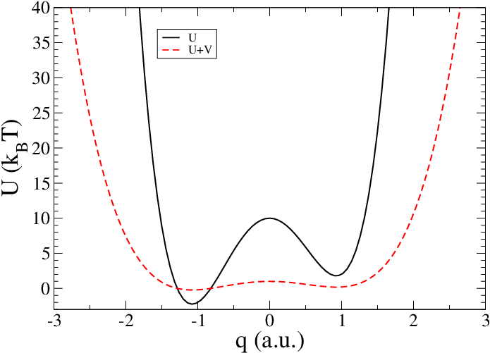
Figure 1: The model 1D potential is shown. Unbiased potential $U$ (solid) and total potential $U+V$ (dashed), as defined in Eqs. 5 and 6. Notice that the barriers is decreased by a factor 10 in the biased potential.

As a first example we discuss a simple one dimensional toy model of a single particle confined into a double well potential. All quantities are here expressed in arbitrary units, and we assume the thermal energy $k_{B}T=1$ and particle mass $m=1$. We consider a potential energy:

$$U\left(q\right)=A\,\left(1-q^{2}\right)^{2}+B\,q^{3},$$ (5)

where $A=10$ and $B=2$. As shown in Fig. 1 such potential has two stable minima which are separated by a barrier of several $k_{B}T$. Transitions are accelerated by means of an umbrella potential Torrie and Valleau (1977) in the form

$$V\left(q\right)=-0.9\,U\left(q\right).$$ (6)

Using a negative fraction of the potential energy as bias potential is convenient because, as it is evident from Fig. 1, it lowers the barriers keeping the system confined into the interesting regions of phase space. Moreover, this choice is consistent with the expected bias potential obtained in the long-time limit in a well-tempered metadynamics simulation Barducci et al. (2008).

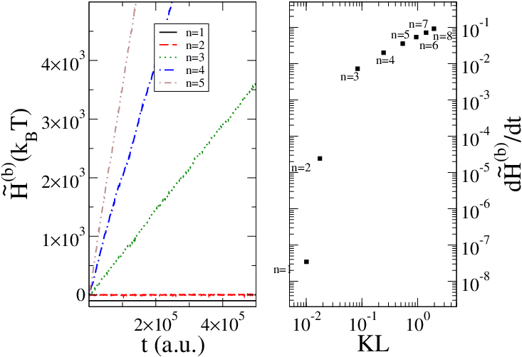
Figure 2: Bias effective energy drift as a function of time (left panel) for different values of the multiple time step order $n$, as indicated. Notice that the line corresponding to $n=1$ has been shifted downward by 100 $k_{B}T$ for clarity. Time derivative of bias effective energy as a function of Kullback–Leibler divergence $D_{KL}$ (right panel) for $n$ ranging from 1 to 8, as indicated. Both the drift and the $D_{KL}$ are growing monotonically with $n$.

The system is then evolved according to a Langevin equation:

$$m\ddot{q}=-\frac{\partial U}{\partial q}-\frac{\partial V}{\partial q}-\gamma m\dot{q}+\sqrt{2\gamma mk_{B}T}\eta(t),$$

with friction $\gamma=1$. Equations are integrated with the scheme proposed in Ref. Bussi and Parrinello (2007), using an inner time step $\Delta t=0.01$. MTS is implemented by scaling the biasing force $-\frac{\partial V}{\partial q}$ by a factor $n$ and by applying it every $n$-th step.

The bias effective energy drift is then computed and shown in Fig. 2 for $n=1$, 2, 3, 4, and 5. Notice that the bias effective energy is clearly drifting for $n>2$, and that its drift is growing with $n$. This is in agreement with the intuitive observation that a larger time step would make the path integral of the forces more and more different from the corresponding potential, as it can be seen in Eq. 3. We observe that the actual value of the drift also depends on the Langevin thermostat and that the drift could be reduced by decreasing the friction $\gamma$ or by integrating the thermostat in the outer time step (see Figs. S1, S2, and S3). However this 1D model is meant to mimic a dimensional reduction of a finer grain model. Thus friction should not be considered as a tunable parameter but as an actual part of the model which depends on how coupled is the biased CV with the other microscopic degrees of freedom.

We also compute the difference between the observed distribution and the theoretical one using the Kullback-Leibler divergence $D_{KL}=\sum_{i}\log\left(\frac{p_{i}}{h_{i}}\right)p_{i}$, where $p_{i}$ is the theoretical distribution and $h_{i}$ is the empirical histogram, both computed with a bin size of 0.01. In Fig. 2 we show the relationship between the slope of the effective energy drift and the Kullback-Leibler divergence. The results clearly show that the effective-energy drift is a good proxy for the sampling error, and can be used in situations where a reference result does not exist so as to simplify the choice of $n$ and to allow errors to be detected.

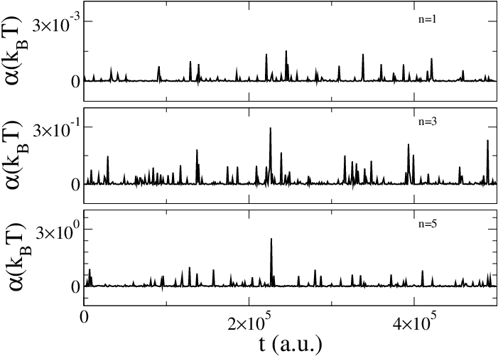
Figure 3: In the three panels neglected terms $\alpha$ (see Eq. 4) for the bias effective energy are shown as a function of time for selected choices of the multiple time step order $n=1,3,5$, as indicated. Although for $n=5$ there are spikes on the order of a few $k_{B}T$, this term does not present any significant drift.

To verify that the neglect of terms related to forces defined in Eq. 4 is not affecting the overall effective energy drift, we compute it explicitly. Figure 3 shows that such a force term only contributes to fluctuations and not to the overall drift.

The tests on this one-dimensional potential were performed using Langevin dynamics. The idea of defining an effective energy drift in a stochastic equation of motion is relatively new.Bussi et al. (2007); Bussi and Parrinello (2007) However, the theoretical considerations discussed in this paper apply to any thermostating procedure, including deterministic ones. As it can be appreciated in Fig. S4, the drift computed using Eq. 3 is close to the one obtained by monitoring the total energy conservation with a conventional Nosé-Hoover thermostat.Nosé (1984); Hoover (1985)

III.2 Dihedral angles in alanine dipeptide

As a second test, we study the free energy surface (FES) of the alanine dipeptide with umbrella sampling simulations, using different values for the multiple time step order $n$. Alanine dipeptide in water is a standard model system for many theoretical and computational studies of biomolecules Rossky et al. (1979), and is known to exhibit multiple minima on the FES computed as a function of the $\phi,\psi$ torsional angles (see Fig. 4). The terminally blocked alanine peptide (sequence Ace-Ala-Nme) was solvated with 542 TIP3P Jorgensen et al. (1983) water molecules in a rhombic dodecahedral box, whose dimensions were chosen to ensure a minimum distance to the box boundaries of 10 Å. Molecular dynamics simulations were performed with the AMBER99SB Hornak et al. (2006) force field using Gromacs 4.6 Hess et al. (2008) in combination with an in house version of PLUMED 2 Tribello et al. (2014). Long range electrostatic forces were treated using particle-mesh Ewald summation Darden et al. (1993), and the equations of motion were integrated with time step $\Delta t=$2 fs. All simulations were performed in the canonical ensemble ($T=300$K) with stochastic velocity rescaling Bussi and Parrinello (2007), and bond lengths were constrained using the LINCS algorithm Hess (2008).

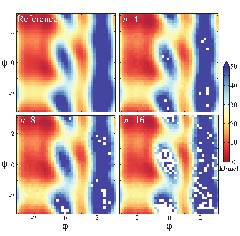
Figure 4: Free energy surfaces of alanine dipeptide projected onto the $\phi,\psi$ dihedral angles obtained from umbrella sampling simulations. The reference FES (top left panel) is compared with results obtained using different stride values of the multiple time step order $n$, as labeled.

We first performed a 100 ns well-tempered metadynamics simulation Laio and Parrinello (2002); Barducci et al. (2008) using the $\phi,\psi$ angles as collective variables. The Gaussian width was set to 0.35 rad, and the deposition interval was 3.2 ps with a starting Gaussian height of 0.4 kJ/mol and a bias factor of 10, corresponding to an enhancement in the CV temperature of $\Delta T=2700$ K. We then used the obtained bias potential to perform an umbrella sampling (US) refinement as in Ref.Babin et al. (2006). A reference free energy landscape was obtained by running a 500ns US simulation with single time step ($n=1$). We then performed a set of 100 ns US simulations using different multiple time step orders $n$, and compared the results with the reference simulation. As for the 1D double-well case, the accuracy on the reconstructed free energy surface decreases for increasing values of $n$ (Fig. 4). The discrepancy is noticeable around the free energy maxima, but much less pronounced in the relevant low-free-energy regions. The agreement between the reference and the MTS simulation with stride $n$ was quantified by calculating the deviation

$$\Delta\Delta F=\Delta F_{REF}-\Delta F_{MTS,n}$$

where $\Delta F_{REF}$ and $\Delta F_{MTS,n}$ are the free energy differences between the region $\phi\in[-\pi,-0.4]$ and the region $\phi\in[0.4,1.6]$ for the reference and the MTS simulation, respectively. As a measure of the error, we additionally computed the deviation from the reference free-energy landscape as

$$\epsilon=\left(\frac{1}{A}\int_{\Gamma}\left[F_{REF}(\phi,\psi)-F_{MTS,n}(\phi,\psi)-C\right]^{2}d\phi d\psi\right)^{\frac{1}{2}}$$

where $\Gamma$ is the region in dihedral space such that $F_{REF}(\phi,\psi)-\min(F_{REF}(\phi,\psi))<25$ kJ/mol and A is the corresponding area. Note that $\Gamma$ includes all the minima as well as the transition states. The value of $C$ is chosen so as to align the averages of $F_{REF}$ and $F_{MTS}$ over $\Gamma$. As shown in Fig. 5A, both $|\Delta\Delta F|$ and $\epsilon$ slowly grow with $n$. Notably, for $n\leq 8$, the error on the free energy estimate is comparable with the statistical fluctuations obtained with $n=1$. The sampling error introduced by the multiple time step can be effectively monitored by considering the bias effective energy drift (Fig. 5B). This is particularly convenient in real-case scenarios, where one does not have a reference simulation to compare with.

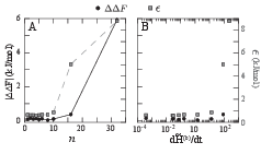
Figure 5: Two different estimates of the sampling error in umbrella sampling simulations of alanine dipeptide, namely free-energy difference between two regions ($\Delta\Delta F$, circles) and average error ($\epsilon$, squares). Left: Sampling error vs multiple time step order. Right: Sampling error vs time derivative of bias effective energy drift.

III.3 Electrostatic energy in a protein/RNA complex

As a third and more realistic test case we consider the calculation of the free-energy landscape using metadynamics on a protein/RNA complex. The nonstructural protein 3 from the Hepatitis C Virus (NS3 HCV) is a motor protein that unwinds and translocates the double and single stranded nucleic acids in the 3’ $\rightarrow$ 5’ direction hydrolyzing ATP Ding and Pyle (2012). Here we compute the free-energy profile of the NS3 helicase complexed with a single stranded RNA, performing a short well-tempered metadynamics. We use here as a collective variable the Debye-Hückel approximation to the electrostatic component of protein/RNA interaction defined as in Ref. Do et al. (2013)

$$G^{DH}=\frac{1}{k_{B}T\epsilon_{w}}\sum_{i\in\text{prot}}\sum_{j\in\text{RNA}}q_{i}q_{j}\frac{e^{-\kappa|\mathbf{r}_{ij}|}}{|\mathbf{r}_{ij}|}$$ (7)

where $\epsilon_{w}$ is the water dielectric constant, $q_{i}$ is the charge of atom $i$, ${\bf r}_{ij}$ is the vector connecting atoms $i$ and $j$ and $1/\kappa$ is the screening length. Here atom indexes $i$ and $j$ run over the protein and RNA respectively. Although we do not characterize protein/RNA binding in this application, this is a prototype setup for the study of complexes of charged molecules (e.g. nucleic acids, charged ligands, etc). All the simulation parameters were the same as for alanine dipeptide, but simulations were performed in the NPT ensemble using a Parrinello-Rahman barostat with an isotropic pressure coupling of 1 bar Parrinello and Rahman (1981) and the AMBER99sb-ILDN* force field Best and Hummer (2009); Lindorff-Larsen et al. (2010) with parmbsc0 and $\chi_{OL3}$ corrections Pérez et al. (2007); Zgarbová et al. (2011). The system was prepared starting from the crystal structure of the complex between the protein and an ssRNA of 6 nucleotides by Appleby et al. Appleby et al. (2011) (PDB: 3O8C). The simulation box contains 100012 atoms, and includes 31058 water molecules and NaCl 0.1 M (70 Na⁺ and 62 Cl^- ions).

The biased CV ($G^{DH}$) was computed using a nominal ionic strength of 0.1M. Protein and RNA here contain respectively $\approx 6500$ and $\approx 180$ atoms, so that the cost of evaluating the CV is relevant. Bias was deposited with a Gaussian width of 0.25 kJ/mol, a bias factor of 2, an initial Gaussian height of 0.1 kJ/mol and a deposition pace of 0.12 ps. The low value of the bias factor was chosen to avoid the complex to dissociate resulting in a difficult-to-converge free-energy landscape. We performed well-tempered metadynamics simulations of 3 ns length testing different values for the multiple time step order ($n=$1,2,3,6). We notice that it is very difficult to obtain a converged free-energy landscape with these very short simulations. However, as it can be seen in Fig. 6, the free-energy landscape obtained after 3 ns is very consistent across simulations performed with values of $n$=1 and 2. On the contrary, with $n=3$ we obtain a clear systematic error in the computed landscape. Remarkably, the calculation with $n=6$ leads again to a relatively small error. The particularly bad case of $n=3$ could be related to resonance effects between the biased CV and the internal degrees of freedom of the system.

Also in this case one can compute the bias effective energy drift for different choices of $n$. It is worth noting that two extra contributions have to be included here in order to compute the effective energy properly, one to take into account the out of equilibrium nature of metadynamics (see Appendix A) and another one to take into account the change in the cell volume due to the barostat at every time step (see Appendix B). As it can be appreciated in Fig. 7, the drift is clearly increasing with $n$. Already at $n=3$ a drift of several tens of kJ/mol/ns can be observed. We notice that electrostatic interaction is not a smooth function of the atomic coordinates. Indeed, in standard MD codes, only its long range tail is sometime integrated using a larger time step. Thus, a large drift for $n=3$ can be expected here. Notably, the drift at $n=2$ is much smaller, consistently with the fact that no systematic error is observed in Fig. 6. This suggest that effective energy conservation is a sufficient criterion to assess the integration with our MTS scheme.

This application can be considered as an example of a realistic system. Performance that can be obtained with this setup are shown in Figure 8. As it can be seen for a highly expensive CV the performance gain can be large. Notably, the contribution to the total calculation time of the calculation of the CVs scales inversely with the MTS order $n$. Even for $n=2$ the gain is significant.

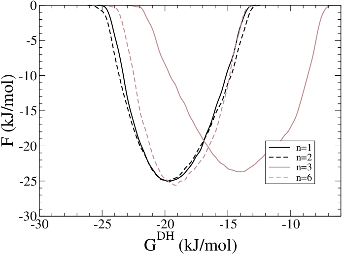
Figure 6: Free-energy profile as a function of the $G^{DH}$ collective variable (see Eq. 7) as obtained from a well-tempered metadynamics performed on the protein/RNA complex. Results from different values of the MTS order $n$ are shown.

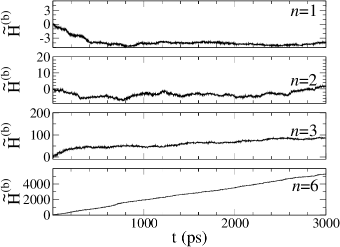
Figure 7: Bias effective energy as a function of time as obtained from a well-tempered metadynamics simulation biasing the $G^{DH}$ collective variable performed on the protein/RNA complex. Results for different values of the MTS order $n$ are shown as indicated. Energies are in kJ/mol.

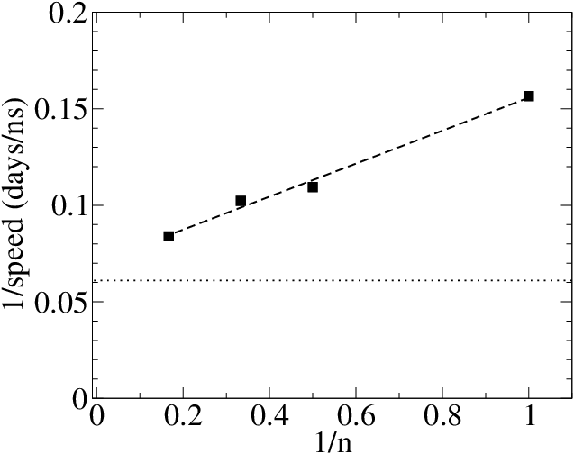
Figure 8: Performance measured on the metadynamics calculation on a protein/RNA complex for different multiple time step orders $n$ (squares), estimated on a GPU-based Linux workstation (CPU: 12 cores Intel E5-2620; GPU: 1 GeForce GTX TITAN). A linear fit is also shown (dashed line). Both force-field calculation and CV calculation were parallelized on 12 threads using OpenMP. Performance without metadynamics is indicated as a horizontal dotted line .

IV Discussion and Conclusions

We presented a scheme based on reversible multiple time step to integrate physical forces and biasing forces using different strides. This can be convenient when biasing collective variables (CVs) that are smooth and computationally expensive, since it allows the CVs to be computed every few steps. The implementation is straightforward, since it just requires biasing forces to be scaled by a factor $n$ equal to the stride used for their calculation. The accuracy of the algorithm is discussed in detail on a one dimensional model and on alanine dipeptide in explicit solvent. Additionally, a protein/RNA complex has been used as a model for a realistic application. Although in this case it is difficult to converge a free-energy landscape within a short simulation, the impact of the introduced algorithm on performance is clear. A multiple time step order $n=2$ has been shown to provide a remarkable speed up without significantly affecting the accuracy of the calculation. We stress that the case of electrostatic interaction is particularly difficult since this CV is not a smooth function of the atomic coordinates. In the alanine dipeptide, where CVs that are smooth functions of the coordinates were employed, values up to $n\approx 8$ where shown to introduce no significant error. In practical applications, different CVs could require different values of $n$ and thus the performance gain could be different. To help the users in this choice, we introduced here a theoretical framework for assessing the accuracy of the explored ensemble. This formalism is very powerful in that it allows an energy drift to be defined that includes selected portions of the potential energy. We here used it to isolate the contribution to the effective energy drift given by the biasing force from the contribution given by the physical forces. This decomposition allows one to focus the assessment to the relevant portion of the potential-energy function, thus avoiding relevant errors to be masked by e.g. solvent fluctuations. In this manner, although sampling errors are not corrected, it is easy to detect improper choice of $n$. Even though it is not possible to define a universal relationship between the drift and the error, it is clear that the effective energy is a powerful tool to validate MTS simulations. Finally, we observe that this check can in principle be used also with a single time step integration scheme ($n=1$) since, also in this case, the forces added by enhanced sampling techniques could be too stiff to be integrated with a conventional time step.

The discussed algorithm has been implemented in a locally modified version of the PLUMED plugin and is available on request. It will be publicly available in the next PLUMED release.

V Appendix A: Out of equilibrium simulations

The effective energy drift provides a rigorous way to asses the validity of detailed balance. However, there are a number of relevant situations where detailed balance is by construction violated during the simulation, e.g. all non equilibrium free-energy techniques Dellago and Hummer (2014). As an example, in steered molecular dynamics Grubmuller et al. (1996) the work can be used to compute free energies Jarzynski (1997) or to reweight the obtained conformations Colizzi and Bussi (2012). However, for the sake of validating the integration of the equations of motion, one can limit the analysis to the portion of work performed by the integrator. In case of steered molecular dynamics the work accumulated by moving the restraint should be removed from the effective energy drift. In a similar fashion, in metadynamics Laio and Parrinello (2002) the sum of the height of the accumulated Gaussians should be subtracted from the effective energy drift.

VI Appendix B: Variable cell simulations

In the case of variable cell simulations Andersen (1980); Parrinello and Rahman (1981) an additional contribution related to cell change should be added to the effective energy drift. Additionally, attention should be paid when computing the increment of positions $\Delta\mathbf{q}$ when particles cross the boundaries. Equation 3 should be replaced with

$$\Delta\tilde{H}^{(b)}(t)=\sum_{i=1}^{N_{at}}\Delta\mathbf{s}_{i}\cdot\left(\frac{\mathbf{g}_{i}^{(b)}(t)+\mathbf{g}_{i}^{(b)}(t+\Delta t)}{2}\right)+\mathrm{tr}\left[\Delta\mathbf{h}^{T}\left(\frac{\mathbf{W}^{(b)}(t)+\mathbf{W}^{(b)}(t+\Delta t)}{2}\right)\right]+\Delta V$$ (8)

where $\mathbf{h}$ is the matrix of lattice vectors (as rows), $\mathbf{s}_{i}=\left(\mathbf{h}^{T}\right)^{-1}\mathbf{q}_{i}$ are the scaled coordinates of $i$-th atom, $\mathbf{g}_{i}=\mathbf{h}\mathbf{f}_{i}$ are the scaled biasing forces on $i$-th atom, and $\mathbf{W}^{(b)}=\frac{\partial V}{\partial\mathbf{h}}$ is related to the bias contribution to the virial tensor. The first term in Eq. 8 is defined in terms of scaled coordinates and forces so as to allow the distance vector $\Delta\mathbf{s}_{i}$ to be evaluated with the minimal image convention when the cell is modified. This term reduces to the first term in Eq. 3 when the cell matrix is constant. The second term is only present for variable cell simulations.

VII Acknowledgement

Michele Ceriotti is acknowledged for carefully reading the manuscript and providing useful suggestions. Alessandro Laio is also acknowledged for useful discussions. The research leading to these results has received funding from the European Research Council under the European Union’s Seventh Framework Programme (FP/2007-2013) / ERC Grant Agreement n. 306662, S-RNA-S.

VIII Supplementary Information

Figures showing the dependence of the bias effective energy drift on the friction coefficient $\gamma$ for the 1D model. Figure showing the effective energy drift for the 1D model using a Nosé-Hoover thermostat.

References

- Allen and Tildesley (1987) Allen, M. P.; Tildesley, D. J. Computer Simulation of Liquids; Oxford University Press: New York, 1987.
- Frenkel and Smit (2002) Frenkel, D.; Smit, B. Understanding Molecular Simulation, 2nd ed.; Academic Press: London, 2002.
- Tuckerman (2010) Tuckerman, M. E. Statistical Mechanics: Theory and Molecular Simulation; Oxford Graduate Texts; Oxford University Press: New York, 2010.
- Dror et al. (2011) Dror, R. O.; Young, C.; Shaw, D. E. In Encyclopedia of Parallel Computing; Padua, D., Ed.; Springer, 2011; pp 60–71.
- Torrie and Valleau (1977) Torrie, G. M.; Valleau, J. P. J. Comput. Phys. 1977, 23, 187–199.
- Darve and Pohorille (2001) Darve, E.; Pohorille, A. J. Chem. Phys. 2001, 115, 9169–9183.
- Laio and Parrinello (2002) Laio, A.; Parrinello, M. Proc. Natl. Acad. Sci. USA 2002, 99, 12562–12566.
- Maragliano and Vanden-Eijnden (2006) Maragliano, L.; Vanden-Eijnden, E. Chem. Phys. Lett. 2006, 426, 168–175.
- Marsili et al. (2006) Marsili, S.; Barducci, A.; Chelli, R.; Procacci, P.; Schettino, V. J. Phys. Chem. B 2006, 110, 14011–14013.
- Barducci et al. (2008) Barducci, A.; Bussi, G.; Parrinello, M. Phys. Rev. Lett. 2008, 100, 020603.
- Abrams and Tuckerman (2008) Abrams, J. B.; Tuckerman, M. E. J. Phys. Chem. B 2008, 112, 15742–15757.
- Laio and Gervasio (2008) Laio, A.; Gervasio, F. L. Rep. Prog. Phys. 2008, 71, 126601–126623.
- Barducci et al. (2011) Barducci, A.; Bonomi, M.; Parrinello, M. Wiley Interdiscip. Rev.: Comput. Mol. Sci. 2011, 1, 826–843.
- Abrams and Bussi (2014) Abrams, C.; Bussi, G. Entropy 2014, 16, 163–199.
- Dellago and Hummer (2014) Dellago, C.; Hummer, G. Entropy 2014, 16, 41–61.
- Steinhardt et al. (1983) Steinhardt, P. J.; Nelson, D. R.; Ronchetti, M. Phys. Rev. B 1983, 28, 784–805.
- Trudu et al. (2006) Trudu, F.; Donadio, D.; Parrinello, M. Phys. Rev. Lett. 2006, 97, 105701.
- Branduardi et al. (2007) Branduardi, D.; Gervasio, F. L.; Parrinello, M. J. Chem. Phys. 2007, 126, 054103.
- Pietrucci and Laio (2009) Pietrucci, F.; Laio, A. J. Chem. Theory Comput. 2009, 5, 2197–2201.
- Spiwok and Králová (2011) Spiwok, V.; Králová, B. J. Chem. Phys. 2011, 135, 224504.
- Pietrucci and Andreoni (2011) Pietrucci, F.; Andreoni, W. Phys. Rev. Lett. 2011, 107, 085504.
- Tribello et al. (2012) Tribello, G. A.; Ceriotti, M.; Parrinello, M. Proc. Natl. Acad. Sci. USA 2012, 109, 5196–5201.
- Do et al. (2013) Do, T. N.; Carloni, P.; Varani, G.; Bussi, G. J. Chem. Theory Comput. 2013, 9, 1720–1730.
- Bonomi et al. (2009) Bonomi, M.; Branduardi, D.; Bussi, G.; Camilloni, C.; Provasi, D.; Raiteri, P.; Donadio, D.; Marinelli, F.; Pietrucci, F.; Broglia, R. A.; Parrinello, M. Comput. Phys. Commun. 2009, 180, 1961–1972.
- Fiorin et al. (2013) Fiorin, G.; Klein, M. L.; Hénin, J. Mol. Phys. 2013, 111, 3345–3362.
- Tribello et al. (2014) Tribello, G. A.; Bonomi, M.; Branduardi, D.; Camilloni, C.; Bussi, G. Comput. Phys. Commun. 2014, 185, 604–613.
- Plimpton (1995) Plimpton, S. J. Comput. Phys. 1995, 117, 1–19.
- Van Der Spoel et al. (2005) Van Der Spoel, D.; Lindahl, E.; Hess, B.; Groenhof, G.; Mark, A. E.; Berendsen, H. J. C. J. Comput. Chem. 2005, 26, 1701–1718.
- Phillips et al. (2005) Phillips, J. C.; Braun, R.; Wang, W.; Gumbart, J.; Tajkhorshid, E.; Villa, E.; Chipot, C.; Skeel, R. D.; Kalé, L.; Schulten, K. J. Comput. Chem. 2005, 26, 1781–802.
- Tuckerman et al. (1992) Tuckerman, M.; Berne, B. J.; Martyna, G. J. J. Chem. Phys. 1992, 97, 1990–2001.
- Sexton and Weingarten (1992) Sexton, J. C.; Weingarten, D. H. Nucl. Phys. B 1992, 380, 665–677.
- Bussi et al. (2007) Bussi, G.; Donadio, D.; Parrinello, M. J. Chem. Phys. 2007, 126, 014101.
- Bussi and Parrinello (2007) Bussi, G.; Parrinello, M. Phys. Rev. E 2007, 75, 056707.
- Cornell et al. (1995) Cornell, W. D.; Cieplak, P.; Bayly, C. I.; Gould, I. R.; Merz, K. M.; Ferguson, D. M.; Spellmeyer, D. C.; Fox, T.; Caldwell, J. W.; Kollman, P. A. J. Am. Chem. Soc. 1995, 117, 5179–5197.
- Biesiadecki and Skeel (1993) Biesiadecki, J. J.; Skeel, R. D. J. Comput. Phys. 1993, 109, 318–328.
- Morrone et al. (2011) Morrone, J. A.; Markland, T. E.; Ceriotti, M.; Berne, B. J. J. Chem. Phys. 2011, 134, 014103.
- Leimkuhler et al. (2013) Leimkuhler, B.; Margul, D. T.; Tuckerman, M. E. Mol. Phys. 2013, 111, 3579–3594.
- Lippert et al. (2013) Lippert, R. A.; Predescu, C.; Ierardi, D. J.; Mackenzie, K. M.; Eastwood, M. P.; Dror, R. O.; Shaw, D. E. J. Chem. Phys. 2013, 139, 164106.
- Leimkuhler and Matthews (2013) Leimkuhler, B.; Matthews, C. AMRX Appl. Math. Res. Express 2013, 2013, 34–56.
- Nosé (1984) Nosé, S. J. Chem. Phys. 1984, 81, 511–519.
- Hoover (1985) Hoover, W. G. Phys. Rev. A 1985, 31, 1695–1697.
- Sivak et al. (2013) Sivak, D. A.; Chodera, J. D.; Crooks, G. E. Phys. Rev. X 2013, 3, 011007.
- Gardiner (2003) Gardiner, C. W. Handbook of Stochastic Methods, 3rd ed.; Springer: Berlin, 2003.
- Rossky et al. (1979) Rossky, P. J.; Karplus, M.; Rahman, A. Biopolymers 1979, 18, 825–854.
- Jorgensen et al. (1983) Jorgensen, W. L.; Chandrasekhar, J.; Madura, J. F.; Impey, R. W.; Klein, M. L. J. Chem. Phys. 1983, 79, 926–935.
- Hornak et al. (2006) Hornak, V.; Abel, R.; Okur, A.; Strockbine, B.; Roitberg, A.; Simmerling, C. Proteins 2006, 65, 712–725.
- Hess et al. (2008) Hess, B.; Kutzner, C.; Van Der Spoel, D.; Lindahl, E. J. Chem. Theory Comput. 2008, 4, 435–447.
- Darden et al. (1993) Darden, T.; York, D.; Pedersen, L. J. Chem. Phys. 1993, 98, 10089–10092.
- Hess (2008) Hess, B. J. Chem. Theory Comput. 2008, 4, 116–122.
- Babin et al. (2006) Babin, V.; Roland, C.; Darden, T. A.; Sagui, C. J. Chem. Phys. 2006, 125, 204909.
- Ding and Pyle (2012) Ding, S. C.; Pyle, A. M. Methods Enzymol. 2012, 511, 131–147.
- Parrinello and Rahman (1981) Parrinello, M.; Rahman, A. J. Appl. Phys. 1981, 52, 7182–7190.
- Best and Hummer (2009) Best, R. B.; Hummer, G. J. Phys. Chem. B 2009, 113, 9004––9015.
- Lindorff-Larsen et al. (2010) Lindorff-Larsen, K.; Piana, S.; Palmo, K.; Maragakis, P.; Klepeis, J. L.; Dror, R. O.; Shaw, D. E. Proteins 2010, 78, 1950–1958.
- Pérez et al. (2007) Pérez, A.; Marchán, I.; Svozil, D.; Sponer, J.; Cheatham III, T. E.; Laughton, C. A.; Orozco, M. Biophys. J. 2007, 92, 3817–3829.
- Zgarbová et al. (2011) Zgarbová, M.; Otyepka, M.; Šponer, J.; Mládek, A.; Banáš, P.; Cheatham, T. E.; Jurečka, P. J. Chem. Theory Comput. 2011, 7, 2886–2902.
- Appleby et al. (2011) Appleby, T. C.; Robert, A.; Fedorova, O.; Pyle, A. M.; Wang, R.; Liu, X.; Brendza, K. M.; Somoza, J. R. J. Mol. Biol. 2011, 405, 1139–1153.
- Grubmuller et al. (1996) Grubmuller, H.; Heymann, B.; Tavan, P. Science 1996, 271, 997–999.
- Jarzynski (1997) Jarzynski, C. Phys. Rev. Lett. 1997, 78, 2690–2693.
- Colizzi and Bussi (2012) Colizzi, F.; Bussi, G. J. Am. Chem. Soc. 2012, 134, 5173–5179.
- Andersen (1980) Andersen, H. C. J. Chem. Phys. 1980, 72, 2384–2393.