Derivation of chemical abundances in star-forming galaxies at intermediate redshift

Abstract

We have studied a sample of 11 blue, luminous, metal-poor galaxies at redshift $0.744<z<0.835$ from the DEEP2 redshift survey. They were selected by the presence of the [OIII] $\lambda 4363$ auroral line and the [OII] $\lambda\lambda 3726,3729$ doublet together with the strong emission nebular [OIII] lines in their spectra from a sample of $\sim 6000$ galaxies within a narrow redshift range. All the spectra have been taken with DEIMOS, which is a multi-slit, double-beam spectrograph which uses slitmasks to allow the spectra from many objects (between 50 and 100 per barrel) to be imaged at the same time. The selected objects present high luminosities ($-20.3<M_{B}<-18.5$), remarkable blue color index, and total oxygen abundances between $7.69$ and $8.15$ which represent 1/3 to 1/10 of the solar value. The wide spectral coverage (from $6500$ to $9100$ Å) of the DEIMOS spectrograph and its high spectral resolution, around ($R$ around $5000$), bring us an opportunity to study the behaviour of these star-forming galaxies at intermediate redshift with high quality spectra.

We put in context our results together with others presented in the literature up to date to try to understand the luminosity-metallicity relation this kind of objects define. The star-forming metal-poor galaxies would be of special relevance in showing the diversity among galaxies of similar luminosities and could serve to understand the processes of galaxy evolution.

By

Jose Manuel Pérez Martínez

UNIVERSIDAD AUTÓNOMA DE MADRID

Department of Theoretical Physics

Master Degree in Theoretical Physics and Astrophysics

Supervised by

Ángeles Díaz Beltrán & Carlos Hoyos Fernández de Córdova

1 Introduction

The chemical evolution of galaxies constitutes the cornerstone to understand the star formation history of galaxies and it is closely related with dynamical galaxy processes such as gas outflows from supernovae and inflows from cosmic accretion. The mean method to measure the chemical abundance of galaxies bases on the analysis of nebular emission lines. Most of these emission lines can be observed in the optical and near infra-red up to redshift of $\thicksim 3$ with current ground and space observatories, but it is not that easy to collect the necessary data to study their properties due to instrument limitations to cover wavelength ranges sufficiently wide.

Measuring the flux ratio of the [OIII]$\lambda 4363$ auroral line against the stronger nebular lines such as [OIII] $\lambda\lambda 4959,5007$ ones will provides one of the most confident ways of determining metal abundances in galaxies. However the detection of the [OIII]$\lambda 4363$ line is difficult since it is very weak in the case of metal-poor galaxies and almost indetectable in metal-rich galaxies. Consequently the detection of [OIII] $\lambda 4363$ is a strong indication of the metal poor content of that object. One galaxy type which commonly presents this feature is the so called blue compact galaxies (BCGs) which were first indentified by Zwicky (1965) as faint emission-line galaxies with UV excess. There exist a considerable interest in the study of low-metallicity galaxies considering that they can enlighten the not well understood first stages of galaxy formation and chemical enrichment (Kunth et al. 2000).

Considerable knowledge about this kind of galaxies came thanks to the images provided by the Hubble Space Telescope (HST) which allow to analyze the different types of objects which form the BCGs: starburst galaxies (Cowie et al. 1991), low luminosity dwarfs at low redshift (Im et al. 1995), low luminosity active galactic nuclei (Tresse et al. 1996) and compact narrow emission-line galaxies (Koo et al. 1994, 1995; Guzmán et al. 1996).

Within galaxies of this kind are the luminous compact blue galaxies (LCBGs) which define those luminous ($M_{B}<-17.5$), compact ($\text{\leavevmode{m}}_{B}\leq 21.0$$mag$$arcseg\text{\textsuperscript{-}\texttwosuperior}$) and blue ($B-V\leq 0.6$) objects undergoing a major star-forming process. In this category are included some starburst galaxies at intermediate redshift and the most luminous BCGs (Hoyos et al. 2004).

The least metal-content galaxies known are I Zw 18 (Searle & Sargent 1972) and SBS0335-052 (Izotov et al. 1990) which have total oxygen abundances of $12+\log(O/H)=7.14$ (Izotov et al. 2006b) and $7.19-7.34$ respectively (Izotov et al. 1990). There have been attempts to rise the metal-poor number of galaxies observed but up to date there are only $\leavevmode\nobreak\ 70$ known galaxies with $12+\log(O/H)\leq 7.65$, most of them in the local universe $z\lesssim 1$.

There are not many observations of metal-poor galaxies at intermediate redshifts (Kobulnicky et al. 2003; Kewley et al. 2004; Hoyos et al. 2005; Kakuzu et al 2007, Ly et al 2014) which suggests that at a given metallicity, galaxies were typically more luminous in the past, while the high redshift samples show subsolar metallicities with lumininosities which exceed the bright of comparable matallicity local galaxies. Although it is expected that the luminosity-metallicity relation evolves with the lifetime of galaxies, the way it does is not well understood. Therefore it is needed to increase the number of metal-poor galaxies studied in order to determine the causes of the chemical abundances behaviour through the galaxy life-time.

In this work I focus in the galaxies contained in the fourth release of DEEP2 galaxy survey with detectable [OIII] $\lambda 4363$ line, with the aim of a) deriving their chemical abundances following the so called “direct method”; and b) studying the metallicty-luminosity relation for galaxies at intermediate redshift ($z\sim 0.7$ to $0.8$). The studied galaxies have been selected by the presence of [OIII] $\lambda 4363$ weak emission line in their spectra together with other oxygen lines such as [OIII] $\lambda\lambda 4959,5007$ and a resolved [OII] $\lambda\lambda 3726,3729$ doublet. These conditions can only be reached with the aid of great deep field telescopes such as the 10m. Keck telescopes in Hawaii.

The outline of the work is as follows. In Section 2, we describe the characteristics of DEIMOS spectrograph and the features and quality of DEEP project spectra. Here is where we present the sample selection process and conditions along with other properties collected such as magnitudes or logarithm mass. We put in context all this information with other galaxies at comparable redshifts of DEEP2 through color-magitude diagrams. We then present in Section 3 our results on the measurement of the emission lines, the derivation of the gaseous electron density and temperature and the computation of ionic and total abundances. In Section 4 we discuss the results obtained constructing a luminosity-metallicity diagrams and studying the ionic oxygen abundance balance versus the metallicity of the sample. In order to explore any possible effects on the derived abundances of the degree of excitation of the nebulae we also compare the data from our sample with previous works on the same type of galaxies. Finally in Section 5 we present the main conclusions of this study.

Throughout this work we assume a flat cosmology with $\text{\leavevmode{W}}_{\text{\leavevmode{L}}}=0.7$, $\text{\leavevmode{W}}_{M}=0.3$ and $H_{0}=70$ $\mbox{$km$}s^{-1}$ $Mpc^{-1}$ to determine distance-dependent measurements. Magnitudes are in the Vega system.

2 Data Selection

2.1 The DEEP project

The Deep Extragalactic Evolutionary Probe (DEEP) is a multi-year program which uses the twin 10-m W.M. Keck Telescopes and the Hubble Space Telescope (HST) to conduct a large-scale survey of distant, faint, field galaxies. The DEEP2 redshift survey is the second stage of DEEP project which use the DEIMOS spectrograph to obtain spectra of $\sim 50.000$ faint galaxies with redshifts $z\gtrsim 0.7$. DEIMOS is a multi-slit, double-beam spectrograph which uses slitmasks to allow the spectra from many objects (between 50 and 100 per barrel) to be imaged onto a mosaic CCD array. Some of the most important features are its wide spectral coverage (from 6500 to 9100 Å) and its high spectral resolution, around $R\sim 5000$.

The survey has been designed to have the reliability of local redshift surveys and to be complementary to others large redshift surveys such as the SDSS project and the 2dF survey. DEEP2 survey observes at four separate sky fields covering approximately three square degrees. Along this area it has detected 52989 galaxies which form the redshift catalog; for each of them the survey provides a one dimensional spectrum split in two images corresponding to the red and blue beam of the instrument. The spectra are grouped according to slitmask number and each slitmask was observed for approximately 1 hour (3 exposures of 1200 seconds each). For the data presented in this work the 1200 lines per mm grating centered at $7800\mathring{A}$ was used, typically covering a wavelength range of $6500-9100\mathring{A}$ depending on slit placement on the mask. The dispersion obtained under these conditions is about 3 pixels per angstrom, which allows deconvolution of usually blended lines such as the [OII] $\lambda\lambda 3726,3729$ doublet.

2.2 Sample selection

Galaxies were selected by inspection of reduced spectra from the DEEP2 redshift survey using several criteria. A selection process over the entire reshift catalog was carried out in order to isolate the fraction of spectra which contains the strong oxygen emission lines [OII]$\lambda 3727$, [OIII]$\lambda 4959$, [OIII]$\lambda 5007$ and the weak auroral line [OIII]$\lambda 4363$. The redshift catalog includes 52989 objects whose spectra cover in average the wavelength range between $6500-9100\mathring{A}$. This means that only a small portion of the survey will have the entire set of lines due to constraints imposed by the redshift value. We can determine the correct redshift range using the accurate redshift measurements provided by DEEP2 along with the spectrum wavelength range mentioned before. In order to get the constraints we need to include the two furthest lines into this range, so that the observed [OII] $\lambda 3727$ line wavelength was longer than $6500\mathring{A}$ while the observed [OIII] $\lambda 4959$ line wavelength was shorter than $9100\mathring{A}$. There is no need to include the [OIII]$\lambda 5007$ in the range since its flux value can easily be computed from the [OIII] $\lambda 4959$ using the theoretical ratio between both lines of 2.98 (Storey and Zeippen 2000).

Thus, the first data sample ready to analyze includes only 6241 galaxies within a redshift range of $0.744<z<0.835$. After this selection process, it was necessary to carry out a visual inspection of each spectrum setting two additional conditions: Firstly we had to determine whether the auroral [OIII]$\lambda 4363$ line is visible in the spectrum or not. This line is crucial to understand the properties of the galaxy such as luminosity, metal-richness and ionization degree, moreover it could bring information about a possible underlying population inside the galaxy (C.Hoyos and A.I. Díaz 2006). The second step is to look for an [OII] $\lambda 3727$ doublet clearly separeted in their two energy levels $\lambda 3726$ and $\lambda 3729$ which will allow us to determine the electron density of the ionized region without making any assumption in contrast with precedent works.

I used the IGI tool of the STSDAS package of Iraf to plot the spectrum in three panels, each of them has at least an oxygen emission line in the center of the chosen wavelength range. This method allows us to perform a rapid visual inspection of each spectrum determining the quality of its line fluxes at first sight. In the case in which we were not capable of seeing the [OIII]$\lambda 4363$ line due to the high noise level noise we discarded the spectrum.

$DEEP2$	$z$	$R.A.$	$Decl.$	$m_{B}$	$M_{B}$	$U-B$	$B-V$	$M_{log}^{(a)}$
$ID$		$(J2000)$	$(J2000)$
13016475	0.74684	14:20:57.85	52:56:41.81	22.30	-19.62	0.03	0.01	9.26
22032252	0.74872	16:53:03.49	34:58:48.95	23.29	-18.55	0.33	0.30	9.35
31019555	0.75523	23:27:20.37	00:05:54.76	23.15	-18.90	-0.30	-0.36	8.34
12012181	0.77166	14:17:54.62	52:30:58.42	22.84	-19.33	0.01	-0.02	9.09
14018918	0.77091	14:21:45.41	53:23:52.70	22.32	-19.62	0.17	0.13	9.48
41059446	0.77439	02:26:21.48	00:48:06.81	21.78	-20.27	0.42	0.34	10.10
41006773	0.78384	02:27:48.87	00:24:40.08	23.47	-18.82	0.08	0.03	8.99
22021909	0.79799	16:50:55.34	34:53:29.88	23.38	-18.90	0.25	0.17	9.26
22020856	0.79448	16:51:31.47	34:53:15.96	22.59	-19.46	0.32	0.23	9.59
22020749	0.79679	16:51:35.22	34:53:39.48	22.59	-19.50	0.38	0.28	9.69
31046514	0.78856	23:27:07.50	00:17:41.50	22.67	-19.30	0.61	0.47	9.94

Table 1: Right ascension, declination, redshift, DEEP2 photometric magnitudes and logarithmic mass of the galaxy sample. All the quantities has been obtained photometrically by blabla

Figure 1: Spectrum of two low metallicity galaxies at redshift z=0.747 and z=0.789 respectively. Both of them show the temperature sensitive [OIII]$\lambda 4363$ line used to identify the sample and the other oxygen emission lines used to measure the ionic and total abundances. Top panels do not present the [OIII]$\lambda 5007$ due to a slit displacement on the mask which reduced the long wavelength limit in which DEIMOS can measure.

The best and worst quality spectra in the final sample are represented in top and down panels of Figure 1 respectivey. As we can see the flux intensity of the Balmer lines is somehow related with the [OIII] flux intensity lines, so that when we find a low signal in $H\text{\leavevmode{g}}$ we expect to have problems measuring the auroral [OIII]$\lambda 4363$ line considering the average noise level of spectra. This will be the greatest difficulty in selecting the final galaxy sample and one of the major error sources in determining the electronic temperatures and oxygen abundances. Finally the visual inspection of the subsample yielded 11 galaxies, wich represent the $0.2$% of the initial sample.

The next step is to characterize the final sample of spectroscopically selected galaxies. We present the photometrically observed and absolute magnitudes for the Johnson B filter in addition to the color index for each object included in the final sample in Table 1. Blue absolute magnitudes ($M_{B}$) and rest frame $U-B$ and $B-V$ colors were calculated from the BRI photometry (Coil et al 2004) with K-corrections following those described by Willmer et al. (2005). The results show that most of the galaxies have $M_{B}\leq 18.5$ with color indexes such as $U-B\lesssim 0.6$ which means we are working with luminous blue galaxies that are undergoing a burst of star formation (Hoyos et al. 2004).

Our final galaxy sample has to be put in context within others galaxies at similar redshift. We have chosen a set of galaxies from the DEEP2 survey which contains 2421 objects at aproximately the same redshift of our work. The size of this DEEP2 sample has been determined selecting only those galaxies whose $EW_{\beta}>10\mathring{A}$. The equivalent width has been obtained from the DEEP2 Automated Line Fitting in 1-D Spectra (Weiner B. 2004). Linefit is a Fortran program designed to make automatic fitting of spectral lines of 1-d spectra, specifically DEEP2 spectra. For each spectrum, it produces an output of line parameters including the EW of every fitted line. This procedure is automated and it works well on emission lines. The results of the comparison between the objects of this work and the Linefit sample can be seen in Figure 2.

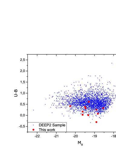
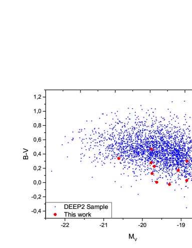
Figure 2: Color-Magnitude diagrams for U, B, and V bands. The DEEP2 sample is composed by 2421 objects in the same interval redshift of this work and with $EW_{\beta}>10\mathring{A}$. Data obtained from DEEP 2 Automated Line Fitting.

The galaxies of this work were found between the bluer and more luminous of the sample. These are common properties between star-forming metal poor galaxies. As we can see in Figure 2, there are not many objects of this kind for such luminosity and redshift.

We will analyze the temperatures, electron densities and oxygen abundances of these galaxies in the following sections.

3 Results

For short wavelength intervals DEIMOS response is essentially constant. This allows us to measure some relative line fluxes without requiring flux calibration of the instrument response. For the analysis of metallicity we have normalized each oxygen emission line to its nearest Balmer decrement in order to determine their relative flux avoiding flux calibrations.

As Hβ and [OIII]$\lambda\lambda 4959,5007$ are very close in wavelength, the DEIMOS response is almost identical, so the relative fluxes remain constant with or without calibration. We can obtain for the same reason the unreddened relative fluxes. since the galactic extinction law doesn’t change too much between nearby wavelengths.

However, it is not possible to use this procedure with the [OII] $\lambda 3727$ doublet since the higher order Balmer decrement could not be measured accurately. Thus the [OII] doublet has to be calibrated and dereddened prior to its measuring as we will see in the following sections.

3.1 Flux Calibration of [OII] $\lambda 3727$ doublet

DEEP2 spectra are not flux calibrated. Hence it is necessary to perform a relative flux calibration over each spectrum. This kind of calibration can be made by studying the performance of the CCD chip to the arrival of photons. We have defined the throughput as the number of photons that are detected at the CCD versus the number of photons that leave the reference object. Three methods were used to measure relative DEIMOS throughput at the DEEP2 survey settings (Konidaris and Koo. 2003), but the basic algorithm is the same in all of them. First of all, it was measured a stellar spectrum with DEIMOS spectrograph, then it has to be determined a “standard” spectrum associated with the measured one, that is, what the measured spectrum should be. Finally the measured spectrum is divided by the standard one so that the result is called throughput. This can be approximated by the following fourth order polynomial:

$$y(\lambda)=-77,9026+0,0395916\lambda-7,49911\times 10^{-6}\lambda^{2}+6,2969\times 10^{-10}\lambda^{3}-1,97967\times 10^{-14}\lambda^{4}$$ (1)

where $\lambda$ is wavelength in Å and y($\lambda$) is in units of $throughput/\mathring{A}$. The throughput is applied to each emission line rate according to the following expression where N is the number of counts of the fitted emission lines:

$$\frac{F_{1}}{F_{2}}=\frac{N_{1}(\lambda_{1})}{N_{2}(\lambda_{2})}\frac{y(\lambda_{2,obs})}{y(\lambda_{1,obs})}$$ (2)

If two lines are very close in wvalength there is no need to use this method because the throughput will be roughly the same. As we will see in the following section, only the [OII] $\lambda 3727$ doublet has been calibrated by this method because there is not any Balmer line close enough to its wavelength. Konidaris and Koo conclude that the associated error to this kind of calibration would be at most 10%.

3.2 Reddening

In the Bohr model of the hydrogen atom there are many different energy levels between which electrons can transfer if they emit or absorb the proper amount of energy. Upward moves require absorption of energy, while downward ones release energy. The Balmer series is characterized by downward electron transitions from levels above the second energy level to second level. When many ionized hydrogen atoms are recombining, as in a planetary nebula where atoms are being ionized and recombining all the time, the captured electrons cascade down through the energy levels. emitting photons of the appropriate wavelengths as they fall. The likelihood of any particular downward jump is dictated by atomic constants. and thus the ratios of all possible transitions can be calculated. This leads to the Balmer decrement, the well known theoretical ratios among the intensities of the Balmer lines.

Thus, the intensity ratios of Balmer lines in all ionized regions should be roughly the same. However, this is not what is observed. Interstellar reddening produced by micron sized dust particles selectively dims shorter wavelength more than it does longer-wavelength, leading to Balmer line ratios that differ systematically from the theoretical predictions. The more dust, the greater the disparity between the observed and theoretical Balmer decrements. From the size of the discrepancy between observed and theoretical Balmer decrements, we can infer the amount of interstellar reddening.

The amount of extinction is parametrized using the logarithmic extinction coefficient c(H$\beta$). It was assumed that the major part of the reddening occurs within the targets objects due to the position of the observation fields and because the observed wavelength are fairly red. Consequently the spectra have been dereddened in the rest frame of the target assuming case B recombination theoretical line ratios. The logarithmic extinction coefficient c(H$\beta$) has been derived using standard nebular analysis techniques (Osterbrock.1989) and assuming the galactic extinction law of Miller & Mathews (1972) with $R_{v}$=3.2. The coefficient has been obtained by taking the difference between the theoretical and observed Balmer decrement available in the espectra and dividing by the normalized extinction curve so that $f(H\beta)=1$. We could only use one Balmer emission line, H$\gamma$, in our sample due to the limited spectral range that the images have at this redshift:

$$\log\left[\frac{I(\lambda)}{I(H\beta)}\right]=\log\left[\frac{F(\lambda)}{F(H\beta)}\right]+c(H\beta)f(\lambda)$$ (3)

$ID$	$z$	$f([OII])$	$f([OIII])$	$f([OIII])$	$f([OIII])$	$EW(H\text{\leavevmode{b}})$	$c(H\text{\leavevmode{b}})$
		$\text{\leavevmode{l}}3727$	$\text{\leavevmode{l}}4363$	$\text{\leavevmode{l}}4959$	$\text{\leavevmode{l}}5007$
13016475	0.7468356	81.9 ± 8.2	8.4 ± 0.3	209.7 ± 2.0	616.9 ± 5.8	161.5	0.48
22032252	0.7487180	134.6 ± 13.7	10.3 ± 1.0	159.5 ± 2.4	452.2 ± 6.7	78.0	0.45
31019555	0.7552315	70.9 ± 7.2	9.5 ± 0.5	176.7 ± 2.3	502.2 ± 5.4	164.9	0.08
12012181	0.7716637	182.3 ± 18.5	14.4 ± 1.1	208.8 ± 3.0	630.7 ± 8.0	41.7	1.23
14018918	0.7709119	187.5 ± 18.8	6.2 ± 0.6	190.0 ± 1.5	578.8 ± 5.7	124.1	0.78
41059446	0.7743866	157.3 ± 15.9	7.7 ± 1.0	167.0 ± 2.0	411.3 ± 5.7	34.8	0.00
41006773	0.7838417	171.9 ± 17.7	12.6 ± 1.4	168.6 ± 3.5	515.9 ± 10.2	36.0	0.98
22021909	0.7979995	133.8 ± 13.5	13.3 ± 0.7	197.6 ± 3.2	598.6 ± 7.1	25.2	0.24
22020856	0.7944890	200.6 ± 20.2	8.0 ± 1.0	160.1 ± 2.1	450.6 ± 5.3	67.7	0.73
22020749	0.7967923	217.3 ± 22	9.7 ± 1.2	125.3 ± 2.6	403.8 ± 6.6	102.3	0.49
31046514	0.7885643	188.9 ± 19.2	6.0 ± 0.7	169.5 ± 3.0	480.2 ± 7.3	47.0	0.85

Table 2: Oxygen emission line fuxes in counts normalized to $f(H\text{\leavevmode{b}})=100$. Rest frame equivalent width of$(H\text{\leavevmode{b}})$ and logarithmic extinction coefficient computed from the $[OII]$ $\lambda 3727$ doublet

3.3 Temperatures and Densities

To compute chemical abundances in ionized gas nebulae, it is required to know the electron temperature. If there were not temperature gradients we could think in an isothermal distribution of the temperature. However the temperature gradients throughout the gas region force us to use the appropiate line temperature for the calculation of each ion. These temperatures can be deduced from the corresponding emission line ratio, but usually not all the lines are accessible in the spectra or have large errors. In these cases, some assumptions are usually adopted concerning the temperaure structure through the nebula. In this work we assume a two phase model with a low ionization zone which depens emission of the [OII] $\lambda 3727$ doublet, and a high ionization zone in which the [OIII] lines are formed.

Now we can determine the values of electron density and temperature from the flux ratios of the observed oxygen emission lines. These ratios are summarized in Table 3.

Ratios
$t_{e}[OIII]$	$R_{O3}=[I(4959)+I(5007)]/I(4363)$
$t_{e}[OII]$	$R_{O2}=I(3727)/[I(7319)+I(7330)]$
$n_{e}[OII]$	$R_{n_{e}[OII]}=I(3726)/I(3729)$

Table 3: Emission-line ratios used to derive electron densities and temperatures

As we said before the ratio which involved the 3727 doublet have the greatest associated error since it had to be calibrated and reddening corrected. We have derived the physical conditions of the ionized gas using the expressions given by Hägele et al. 2008 for the oxygen emission lines of HII galaxies. These formulas are approximate expressions for the statistical equilibrium model in a five levels atom. We present below the adequate fitting functions they used from the TEMDEN task of IRAF, which is based on the program FIVEL (De Robertis, Dufour & Hunt 1987; Shaw & Dufour 1995):

$$t_{e}([OIII])=0.8254-0.0002415R_{O3}+\frac{47.77}{R_{O3}}$$ (4)

$$t_{e}([OII])=0.23+0.0017R_{O2}+\frac{38.3}{R_{O2}}+f_{1}(n_{e})$$ (5)

Since we do not have all the oxygen lines in the allowed spectral range, e.g. $[OII]\lambda\lambda 7319,7330$, it was necessary to calculate $t_{e}[OII]$ from $t_{e}[OIII]$ using Stasinska models as presented in Pagel et al. (1992):

$$t_{e}([OII])\text{\textsuperscript{-}\textonesuperior}=0.5(t_{e}[OIII]\text{\textsuperscript{-}\textonesuperior}+0.8)$$ (6)

This expression is the result of an experimental fitting over the theoretical models proposed by Stasinka in 1990. We are treating with star forming galaxies in which we expect to find high temperature ionized regions. Typically the [OIII] electron temperature is expected to be greater than the [OII] temperature since the first comes from the hotter part of the star-forming region while the second come from the colder regions. Errors in the measurements of $t_{e}[OII]$ are normally higher than the $t_{e}[OIII]$ ones due to the electronic density dependence of the [OII] lines. However, the $t_{e}[OII]$ erros in our sample will be lower considering that we are using the relation between both electron temperatures through the Stasinska model so $t_{e}[OII]$ depends exclusively of the $t_{e}[OIII]$ value. This assumption can or can not be a good approximation depending of the density nebular conditions. Since the assumed state of these regions agrees with the case B recombination phase with temperature around $10\text{\textsuperscript{4}}K$ and density around $100cm\text{\textsuperscript{-}\textthreesuperior}$, we can neglect the density effects over $t_{e}[OII]$ and rely on the Stasinska model.

The derivation of $R_{O3}$ ratio is more complex than in other cases because it involves lines that are widely separate through the spectrum, and therefore they have different response function from DEIMOS spectrograph. As mentioned in section 2, the relative flux of each oxygen line has been measured relative to its nearest Balmer decrement, so that for $[OIII]\lambda 4363$ we measure respect to $H\gamma$ while for the relative flux measurements of [OIII]$\lambda\lambda 4959,5007$ lines we used $H\beta$. To obtain the correct $R_{O3}$ratio we assume the theoretical value between the used Balmer lines obtaining $H\gamma/H\beta=0.471$ (assuming case B recombination). This way we obtain an expression for the $R_{O3}$ ratio minimizing the associated errors of the DEIMOS flux calibration $H\beta$:

$$R_{O3}=\frac{\frac{f(4959)+f(5007)}{f(H\beta)}}{\frac{f(4363)}{f(H\gamma)}}\frac{I(H\gamma)}{I(H\beta)}$$

This method allow us to compute the electronic temperature with deviations not bigger than 5% in the most of cases. Table 4 shows the results for the electron density and temperature. The objects with $t_{e}[OII]\sim t_{e}[OIII]$ are two exceptions since their ionization structure differs from the expected for this type of objects. The difference between the values of $t_{e}([OIII])$ and $t_{e}([OII])$ is slight enough to be overlapped by the predicted errors. The density of the sample remains in its expected value around $100cm\text{\textsuperscript{-}\textthreesuperior}$, far away from the critical oxygen density values, which confirms our assumptions about Stasinska model for this type of objects.

$ID$	$R_{n_{e}[OII]}$	$n_{e}([OII])$	$t_{e}([OIII])$	$t_{e}([OII])$
13016475	0.849	202$\pm$52	1.285 ± 0.020	1.267 ± 0.010
22032252	0.711	$\leq$50	1.612 ± 0.084	1.408 ± 0.032
31019555	0.863	225$\pm$50	1.475 ± 0.040	1.353 ± 0.017
12012181	0.734	70	1.632 ± 0.066	1.416 ± 0.025
14018918	0.835	183$\pm$78	1.179 ± 0.042	1.213 ± 0.022
41059446	0.768	109$\pm$53	1.444 ± 0.086	1.340 ± 0.037
41006773	0.794	142$\pm$75	1.693 ± 0.104	1.438 ± 0.038
22021909	0.687	$\leq$50	1.609 ± 0.050	1.407 ± 0.019
22020856	0.793	138$\pm$72	1.435 ± 0.078	1.336 ± 0.034
22020749	0.743	81$\pm$53	1.691 ± 0.116	1.438 ± 0.042
31046514	0.740	77$\pm$42	1.239 ± 0.054	1.245 ± 0.027

Table 4: Oxygen temperatures and densities for the galaxy sample. The temperature is given in units of $10\text{\textsuperscript{4}}K$ while the density is in $cm\text{\textsuperscript{-}\textthreesuperior}$.

3.4 Chemical Abundances

Abundances refer to the relative proportions of atomic species in the gas phase nebula and these are usually expressed relative to Hydrogen.

The stimation of the metallicity of the emitting nebula is one of the main goals of any nebular analysis. The metallicity of the ionized gas in a galaxy allows us to know the updated chemical composition of the most recent generation of the stars born in the galaxy studied (C. Hoyos 2006). Oxygen is particularly important considering that ionic species of O found in nebulae have strong optical and near ultraviolet emission lines, and it acts as a coolant in most nebulae.

In order to determine the oxygen ionic abundances it was necessary the measurement of two emission line ratios, $\mbox{[OII]}\lambda\lambda 3726+3729/H\beta$ and [OIII] $\lambda\lambda 4959+5007/H\beta$. We used again the fitted expressions given by Hägele et al. 2008 for the oxygen emission lines in HII galaxies in order to compute the ionic abundances. In this case they fitted the IONIC task of IRAF which is based on the program FIVEL (De Robertis, Dufour & Hunt 1987; Shaw & Dufour 1995):

$$12+log(O^{+}/H^{+})=log\frac{I(3726+3729)}{I(H\beta)}+5.992+\frac{1.583}{t_{e}[OII]}-0,681log(t_{e}[OII])+log(1+2.3n_{e})$$ (7)

$$12+log(O^{++}/H^{+})=log\frac{I(4959+5007)}{I(H\beta)}+6.144+\frac{1.251}{t_{e}[OIII]}-0.550log(t_{e}[OIII])$$ (8)

The main problem with the abundance results resides in the method used to get the [OII] temperature. As we stated before our spectral range does not allow us to observe all the necessary [OII] lines to compute $t_{e}[OII].$ That is the reason why we used the Stasinska method, with the assumption of an ionization structure composed of only two phases ([OIII] and [OII]) for these objects.

The metallicity of the galaxies is one of the most important properties to measure if we want to understand their evolutionary behaviour. THe total oxygen abundance is a common way to compute the metallicity of metal-poor galaxies, but prior to measure the total oxygen abundance we have to measure the abundances of all its ions. Since the most abundant ions of oxygen in this regions are $O^{+}$and $O^{2+}$, we can determine the oxygen total abundance as:

$$\frac{O}{H}=\left(\frac{O^{+}}{H^{+}}\right)+\left(\frac{O^{2+}}{H^{+}}\right)$$ (9)

In Tabla 5 we provide the resultant oxygen ionic and total abundances and the ratio between oxygen ionization states ($\log(O\text{\textsuperscript{+}\textsuperscript{+}$/O{{}^{+}}$)}$ in the nebula. The errors are smaller than 0.1 dex for the oxygen ionic and total abundances and between $0.1$ and $0.15$ dex for the $[OIII]/[OII]$ ratio. The results obtained shows low oxygen abundances with metallicities fron 1/3 to 1/10 of the solar value. These results together with the color-magnitude diagrams allow us to confirm that our galaxy sample is indeeed formed by metal-poor galaxies.

$ID$	$12+log(O\text{\textsuperscript{+}}/H\text{\textsuperscript{+}})$	$12+log(O\text{\textsuperscript{+}\textsuperscript{+}}/H\text{\textsuperscript{+}})$	$12+log(O/H)$	$log(O{{}^{+}}{{}^{+}}/O{{}^{+}})$
13016475	7.08 ± 0.06	7.97 ± 0.02	8.03 ± 0.02	0.89 ± 0.08
22032252	7.14 ± 0.08	7.6 ± 0.06	7.73 ± 0.06	0.46 ± 0.13
31019555	6.92 ± 0.06	7.74 ± 0.03	7.80 ± 0.04	0.82 ± 0.09
12012181	7.27 ± 0.07	7.71 ± 0.04	7.84 ± 0.05	0.44 ± 0.11
14018918	7.51 ± 0.07	8.04 ± 0.05	8.15 ± 0.05	0.53 ± 0.12
41059446	7.28 ± 0.08	7.74 ± 0.07	7.87 ± 0.07	0.46 ± 0.15
41006773	7.22 ± 0.08	7.58 ± 0.06	7.74 ± 0.07	0.36 ± 0.14
22021909	7.14 ± 0.06	7.7 ± 0.03	7.81 ± 0.04	0.56 ± 0.10
22020856	7.39 ± 0.08	7.73 ± 0.06	7.89 ± 0.07	0.34 ± 0.14
22020749	7.32 ± 0.08	7.45 ± 0.07	7.69 ± 0.08	0.13 ± 0.16
31046514	7.48 ± 0.08	7.93 ± 0.06	8.06 ± 0.06	0.45 ± 0.14

Table 5: Oxygen ionic and total abundances of the selected galaxy sample in section 2. We enclose as well the ionic abundance ratio which denotes the prevalence of the [OIII] ionic state in the gas region.

4 Discussion

The main result of this work can be seen in Figure 3 where we compare different sets of metal-poor galaxies in a metallicity-luminosity diagram. This figure shows the total oxygen abundance for the 11 galaxies in our sample which is between 1/3 and 1/10 of the solar value of $12+\log[O/H]_{\odot}$=8.69 (Allende Prieto et al. 2001). We compare our sample with other similar ones: Hoyos et al. (2005, hereafter H05), Kakuzu et al. (2007, hereafter K07), Salzer et al. (2009, hereafter S09), Amorín et al. (2014, hereafter A14) and Ly et al. (2014, here after L14) which, as far as I know, represent the almost total comparable information in the literature. It can be seen that our data are in good agreement with these previous works.

The sample from A14 is composed by extreme emission line galaxies (EELGs) selected from the 20k zCOSMOS Bright Survey by their unusually large [OIII] $\lambda 5007$ equivalente widths. They are seven purely star-forming galaxies with the [OIII] $\lambda 4363$ line in their spectrawith redshifts from $z=0.43$ to $0.63$.

The sample from K07 was collected from spectroscopic observations of 161 Ultra strong emission line galaxies (USELs) using the DEIMOS spectrograph on the Keck II telescope. The galaxies are spread in a wide range of redshifts ($0.38<z<0.83$) but is clearly biased towards low metallicities (in some cases with values below that of I Zw 18) and the major part of the sample has low luminosity values. Within this sample are found some objects with quoted electron temperatures higher than 20000K and up to $30000K$ which can not be explained as having normal hiot stars as the only source of ionization. No diagnostic diagrams are provided in order to decide if these objects show any contribution by an AGN or shock heating. If this contribution were important, the nature of the galaxy emission lines in K07 sample would be contaminated and different to the others presented in Figure 3. As a conservative approach, these data should be excluded of the luminosity-metallicity relation. We suggest to reobserve these objects in future works.

The sample from S09 presents some of the most luminous objects of this type ($-22<M_{B}<-20$) at intermediate redshifts ($0.35<z<0.41$) and cover a wide range of the oxygen metallicty of the entire sample. The star-forming galaxies of the KISS sample are derived from a wide-field Schmidt survey that selects emission line objects via the presence of $H\alpha$ emission in their objective-prism spectra (Salzer et al. 2000). The selection process includes a filter that restricted the wavelength coverage of the slitless spectra to $6400-7200$$\AA$. As we move towards higher redshift the bandpass allows to detect objects with other strong emission lines such as [OIII]$\lambda 5007$ due to the shift of its wavelength. Some of the objects selected by this criteria are presented in the left area of Figure 3.

The sample from L14 encompasses a wide luminosity range (from $M_{B}=-21,1$ to $-17.5)$ with abundances going from extreme metal poor galaxies ($12+\log(O/H)\lesssim 7,65$) to galaxies with almost solar abundances. In addition the redshift dispersion of the sample is similar to the one shown in K07$(0.38<z<0.83)$ what provides a good chance to observe star-forming galaxy properties at different ages. The data has been gathered using optical spectroscopy with DEIMOS and MMT’s hectospec spectrographs.

The sample from H05 and this work have many features in common since both of them have been taken from the DEEP2 redshift survey with the DEIMOS spectrograph. Both samples cover the central region of the diagram and have smaller dispersion and smaller errors than the others. The accuracy of this work has been improved respect to H05 results thanks to the measurement of the [OII]$\lambda\lambda 3726,3729$ doublet, which allows to compute directly the nebular electron density and the O⁺/H⁺ ionic abundance with error bars below 0.1 dex as we can see in Figure 3. The redshift range of the H05 sample goes from $z=0.51$ to $0.85$ while in this work the redshift is more restricted ($0.744<z<0.835)$ due to the [OII] line detection requirements.

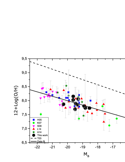
Figure 3: The Luminosity-Metallicity Diagram for intermediate star-forming galaxies for objects of this study and comparable samples from the literature. H05 includes 15 luminous star-forming galaxies from DEEP2. K07 includes 8 EELGs 6 of them are extremely low metallicity galaxies. S09 includes 13 metal-poor galaxies. A14 includes 7 EELGs. L14 includes 17 metal-poor objects. This work presents 11 new metal-poor galaxies. The dashed line on the upper zone of the diagrama represents the Tremonti luminosity-metallicity relation for local SDSS galaxies (Tremonti et al. 2004, T04 in the diagram) while the solid line represents the best fit to all the objects collected.

It can be seen from the figure that both relations show an offset between them. The fit for the Tremonti L-Z relation, for SDSS galaxies with a redshift distribution around $z\sim 0.08,$ and the one obtained in this work for the various collected samples of metal-poor galaxies at intermediate redshift $(0.4<z<0.8),$are respectively given below:

$$12+\log(O/H)=-0.185(\pm 0.001)M_{B}+5.238(\pm 0.018)$$ (10)

$$12+\log(O/H)=-0.158(\pm 0.020)M_{B}+4.842(\pm 0.381)$$ (11)

Our results seem to follow a linear relation between logarithmic oxygen abundance and absolute magnitude with a slope similar to that of T04 but with an offset of about 1.0 dex in abundance, wich can be due to the different nature of the objects involved, selection effects regarding both luminosity and cehmical abundances, or a genuine evolutionary effect. Further work is needed to obtained a Mass-Metallicity relation which can be more free of selection effects.

A hint on the similar or different nature of the objects in our various considered samples can be obtained by looking at the oxygen ionization fractions which reflect the ionization structure of the nebulae. Figure 4 shows the logarithmic ratio between the O²⁺ and O⁺ ionic abundances as a function of the total oxygen abundance. A general trend of decreasing ionization degree (lower O²⁺/O⁺ fraction) with increasing metallicity is expected from the cooling of the gas. This trend is present in the figure, although with a scatter which is larger tahn observational errors. Some degeneracy is found with objects of similar metallicity and widely different ionization conditions. Again further work and more data are needed in order to explore these effects.

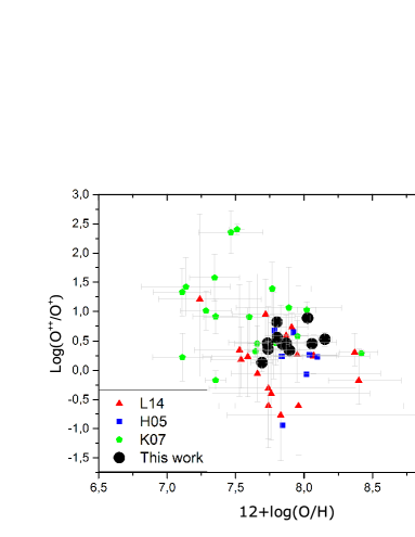
Figure 4: Oxygen ionic fraction as a function of metallicity for the three galaxy samples for wich this information can be derived, together with the objects of this work. A general trend of decreasing ionization degree with increasing metallicity is present along with a strong degeneracy effect in the metallicity with large scatter.

The logarithmic ratio of the [OIII]/[OII] lines is often used as a functional parameter to represent the degree of nebular excitation and can also be used to characterised the different samples involved. Figure 5 shows this ratio ($O_{32}=([OIII]\lambda 4959+\lambda 5007)/[OII]\lambda 3727$) as a function of logarithmic oxygen abundance. Taking figures 4 and 5 together, we can see that a relation between the $O_{32}$ parameter an the oxygen ionic fraction is questionable. In particular, the fact that all the the K07 objects show a very similar value of $O_{32}$ (between 0 and 0.4) spanning, in contrast, a wide range of metallicities. This results together with the mentioned too high temperatures of many objects of the K07 sample reinforce our assumption of an alternative heating process for this objects, since a contribution by shocks will enhance the [OII] emission thus providing an artificially low values of $O_{32}$.

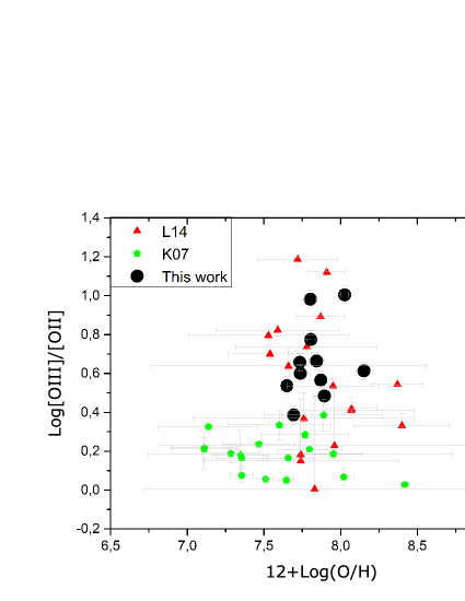
Figure 5: Logarithmic $O_{32}$ emission line ratio as a function of metallicity for the three galaxy samples for which this ratio can be computed.

5 Conclusions

We have studied 11 luminous, blue, and metal poor (1/3 to 1/10 of the solar metallicity) galaxies from DEEP2 survey at redshift $0.744<z<0.835$. The sample was selected by the presence of the [OIII] $\lambda 4363$ auroral line and the [OII] $\lambda\lambda 3726,3729$ doublet together with the strong [OIII] emission lines. These objects represent the $0.002\%$ of the total galaxies within the same redshift interval in the DEEP2 survey what means that these objects are rare, although they are of special relevance to understand the processes of galaxy evolution.

The computed total oxygen abundances $($between $7.69$ and $8.15)$ do not differ so much from those published by Hoyos et al. (2005), but these works together with other such as Ly et al. 2014 constitute the only available and comparable data for objects of this type. In the Luminosity-Metallicty diagram, galaxies of intermediate redshift define a linear relation between logarithmic oxygen abundance and absolute magnitude, arise a linear relation which is almost pararell to the one proposed by Tremonti et al. (2004) for SDSS local objects, but is offset by 1 dex to lower metallicity values.

The ionization structure of the analyzed samples show a general trend of decreasing ionization degree (lower O²⁺/O⁺ fraction) with increasing metallicity which is expected from the cooling of the gas. This trend can be seen in Figure 4, although with a larger scatter than the observational errors. Taking the results of this work together with those presented in L14 and K07, we conclude that the relation between the $O_{32}$ parameter and the oxygen ionic fraction is questionable for metal-poor galaxies since we observed degeneracy effects between objects of similar metallicity and widely different ionization conditions.

Regardless of the cause, metal-poor star-forming galaxies are highly interesting objects whose study is indispensable to understand tke processes of galaxy evolution in time.

References

- [1] Amorín, R. et al. 2014 arXiv:1403-3441v1 [astro-ph.CO]
- [2] Allende Prieto, C., Lambert, D. L., & Asplund, M. 2001, ApJ, 556, L63
- [3] Cowie, L. L., Songaila, A., & Hu, E. M. 1991, Nature, 354, 460
- [4] Coil, A. L., Newman, J. A., Kaiser, N., Davis, M., Ma, C., Kocevski, D. D., & Koo, D. C. 2004, ApJ, 617, 765
- [5] De Robertis, M., Dufour, R. J., & Hunt, R. 1987, JRASC, 81, 195
- [6] Guzman, R., Koo, D. C., Faber, S. M., Illingworth, G. D., Takamiya, M., Kron, R. G., & Bershady, M. A. 1996, ApJ, 460, L5
- [7] Hägele, G. F., Díaz, A. I., Terlevich, E., Terlevich, R., Perez-Montero, E., & Cardaci, M. V., 2008, MNRAS, 383, 209
- [8] Hoyos, C., & Dıaz, A. I. 2006, MNRAS, 365, 454
- [9] Hoyos, Koo, Phillips, Willmer, & Guhathakurta, E.M. 2005, ApJ, 635, l21
- [10] Hoyos, C., Guzman, R., Bershady, M. A., Koo, D. C., & Dıaz, A. I. 2004, AJ, 128, 1541
- [11] Izotov, Y. I., Guseva, N. G., Lipovetsky, V. A., Kniazev, A. Y., & Stepanian, J. A. 1990, Nature, 343, 238
- [12] Izotov, Y. I., Papaderos, P., Guseva, N. G., Fricke, K. J., & Thuan, T. X. 2006, A&A, 454, 137
- [13] Kakazu, Y., Cowie, L. L., & Hu, E. M. 2007, ApJ, 668, 853
- [14] Kewley, Lisa J.; Geller, Margaret J.; Jansen, Rolf A. 2004, AJ, 127, 2002
- [15] Kobulnicky, Henry A.; Willmer, Christopher N. A.; Phillips, Andrew C.; Koo, David C.; Faber, S. M.; Weiner, Benjamin J.; Sarajedini, Vicki L.; Simard, Luc; Vogt, Nichole P. 2003, ApJ, 599, 1006
- [16] Konidaris, N., & Koo, D. C., Brief Memo on DEEP2 Flux Calibrations, 2003
- [17] Koo, D. C., Bershady, M. A., Wirth, G. D., Stanford, S. A., & Majewski, S. R. 1994, ApJ, 427, L9
- [18] Koo, D. C., Guzman, R., Faber, S. M., Illingworth, G. D., Bershady, M. A., Kron, R. G., & Takamiya, M. 1995, ApJ, 440, L49
- [19] Kunth, D., & Ostlin, G. 2000, A&A Rev., 10, 1
- [20] Ly, C., Malkan, M. A., Nagao, T., et al. 2014, ApJ, 780, 122
- [21] Osterbrock, D. E. 1989, Astrophysics of Gaseous Nebulae and Active Galactic Nuclei (Mill Valley: University Science Books)
- [22] Pagel, B. E. J., Simonson, E. A., Terlevich, R. J., & Edmunds, M. G. 1992, MNRAS, 255, 325
- [23] Perez-Montero, E., & Dıaz, A. I. 2003, MNRAS, 346, 105
- [24] Salzer, J. J., Williams, A. L., & Gronwall, C. 2009, ApJ, 695, L67
- [25] Shaw, R. A., & Dufour, R. J. 1995, PASP, 107, 896 (SD95)
- [26] Stasińska, G. 1990 A&AS, 83, 501s
- [27] Storey, P. J.; Zeippen, C. J. 2000, 312, 813
- [28] Tresse L, Rola C, Hammer F, Stasinska G, and LeFevre O, et al. 1996. MNRAS 281:847-70
- [29] Tremonti, C. A., et al. 2004, ApJ, 613, 898
- [30] Zwicky, F. 1965, ApJ, 142, 1293