Fully Dynamic Algorithms for All Pairs All Shortest Paths and Betweenness Centrality

Abstract

We consider the all pairs all shortest paths (APASP) problem, which maintains all of the multiple shortest paths for every vertex pair in a directed graph $G=(V,E)$ with a positive real weight on each edge. We present fully dynamic algorithms for this problem in which an update supports either weight increases or weight decreases on a subset of edges incident to a vertex.

Our basic algorithm runs in amortized $O({\nu^{*}}^{2}\cdot\log^{3}n)$ time per update, where $n=|V|$, and ${\nu^{*}}$ bounds the number of edges that lie on shortest paths through any single vertex. Our method is a generalization and a variant of the fully dynamic algorithm of Demetrescu and Italiano [8] for unique shortest paths (APSP), and it builds on recent work on increase-only APASP [21]. Our algorithm matches the fully dynamic amortized bound in [8] (which works only for single shortest paths) for graphs with $O(n)$-size shortest path dags, though our method, and especially its analysis, are different. We also present a faster APASP algorithm where we achieve an amortized $O({\nu^{*}}^{2}\cdot\log^{2}n)$ time per update. Our faster algorithm uses new data structures and techniques that are extensions of the method in the fully dynamic algorithm in Thorup [27] for APSP in graphs with unique shortest paths.

Our APASP algorithms lead to fully dynamic computation, with the same respective amortized bounds, for betweenness centrality, which is a parameter widely used in the analysis of large complex networks. Moreover, it provides an alternate amortized analysis for the fully dynamic APSP algorithm of Demetrescu and Italiano, and new algorithms for computing APSP under fully dynamic updates.

1 Introduction

Given a directed graph $G=(V,E)$ with positive edge weights, we consider the problem of maintaining APASP (all pairs all shortest paths) [21], i.e., the set of all shortest paths (SPs) between all pairs of vertices. This is a fundamental graph property, and it also enables the efficient computation of betweenness centrality for every vertex in the graph.

Betweenness centrality (BC) is a widely used measure for the analysis of social networks. Shortest paths starting from a node $s$ can be represented by the single source shortest paths (SSSP) out-dag (paths from the root $s$ to the leaves of the dag) rooted at $s$, similarly the shortest paths ending in $t$ can be represented by the SSSP in-dag (paths from the leaves to the root $t$ of the dag) rooted at $t$. In the following, we will refer to these as SP in-dag and SP out-dag.

In this paper we present a fully dynamic algorithm for the APASP problem, where each update in $G$ is either decrease-only or increase-only. A decrease-only update either inserts a new vertex along with incident edges of finite weight, or decreases the weights of some existing edges incident on a vertex. An increase-only update deletes an existing vertex, or increases the weights of some edges incident on a vertex.

Recently, we gave (with Nasre) a simple decrease-only APASP algorithm [20], and a more involved increase-only APASP algorithm [21]. Neither of these algorithms is correct for the fully dynamic case. The fully dynamic methods that we present in this paper build on [21], and also incorporate a variant of the fully dynamic methods developed by Demetrescu and Italiano [8] (the DI method) and Thorup [27] (the Thorup method) for APSP where only one shortest path is maintained for each pair of vertices. The DI algorithm runs in $O(n^{2}\cdot\log^{3}n)$ amortized time per update, where $n=|V|$. The Thorup algorithm is faster by a logarithmic factor but is considerably more complicated, even for the unique shortest paths case. The algorithms in both [8] and [27] use the unique shortest paths assumption crucially, and need considerable enhancements even to maintain a small number of multiple shortest paths correctly. In [28] the author presented a worst case fully dynamic algorithm for APSP which recomputes the complete distance matrix in $\tilde{O}(n^{2.75})$. Recently, the worst case time bound was improved in [1] with a randomized algorithm which runs in $O(n^{2+2/3}\log^{4/3}n)$.

In this paper we present two fully dynamic algorithms for APASP, which maintain all of the multiple shortest paths for every pair of vertices. Our basic algorithm is as simple as the DI method (though somewhat different) when specialized to unique shortest paths. In fact, it matches the DI bound for graphs with a constant number of (or unique) shortest paths, while being applicable to the more general APASP problem. Moreover, it provides a new amortized analysis for the fully dynamic DI algorithm if our ‘dummy sequence’ replaces the one used in DI. Our second algorithm improves the amortized time bound by a logarithmic factor using data structures and techniques that are considerably more complicated.

Both APASP methods give fully dynamic algorithms for the betweenness centrality (BC) problem, described below.

Betweenness Centrality (BC). Betweenness centrality is a widely-used measure in the analysis of large complex networks, and is defined as follows. For any pair $x,y$ in $V$, let $\sigma_{xy}$ denote the number of shortest paths from $x$ to $y$ in $G$, and let $\sigma_{xy}(v)$ denote the number of shortest paths from $x$ to $y$ in $G$ that pass through $v$. Then, $BC(v)=\sum_{s\neq v,t\neq v}\frac{\sigma_{st}(v)}{\sigma_{st}}$. This measure is often used as an index that determines the relative importance of $v$ in the network. Some applications of BC include analyzing social interaction networks [14], identifying lethality in biological networks [18], and identifying key actors in terrorist networks [6, 16].

Heuristics for dynamic betweenness centrality with good experimental performance are given in [11, 17, 10], but none of these heuristics provably improve on the widely used static algorithm by Brandes [5], which runs in $O(mn+n^{2}\log n)$ time (where $m=|E|)$ on any class of graphs. The only earlier results that provably improve on Brandes on some classes of graphs are the recent separate decrease-only and increase-only algorithms in [20, 21]. Table I contains a summary of these results.

The results in this paper are mainly for fully-dynamic APASP, which is an important graph-theoretic property of independent interest. However, we show that our fully dynamic APASP algorithms give fully-dynamic BC algorithms with the same bounds.

Paper		Time	Weights	Update Type	DR/UN	Result
Brandes [5]		$O(mn)$	NO	Static Alg.	Both	Exact
Brandes [5]		$O(mn+n^{2}\log n)$	YES	Static Alg.	Both	Exact
Geisberger et al. [9]		Heuristic	YES	Static Alg.	Both	Approx.
Riondato et al. [24]		depends on $\epsilon$	YES	Static Alg.	Both	$\epsilon$-Approx.
Semi Dynamic
Green et al. [11]		$O(mn)$	NO	Edge Inc.	Both	Exact
Kas et al. [13]		Heuristic	YES	Edge Inc.	Both	Exact
NPR [20]		$O({\nu^{*}}\cdot n)$	YES	Vertex Inc.	Both	Exact
NPRdec [21]		$O({\nu^{*}}^{2}\cdot\log n)$	YES	Vertex Dec.	Both	Exact
Bergamini et al. [4]		depends on $\epsilon$	YES	Batch (edges) Inc.	Both	$\epsilon$-Approx.
Fully Dynamic
Lee et al. [17]		Heuristic	NO	Edge Update	UN	Exact
Singh et al. [10]		Heuristic	NO	Vertex Update	UN	Exact
Kourtellis+ [15]		$O(mn)$	NO	Edge Update	Both	Exact
Bergamini et al. [3]		depends on $\epsilon$	YES	Batch (edges)	UN	$\epsilon$-Approx.
This paper (Basic)		${O({\nu^{*}}^{2}\cdot\log^{3}n)}$	YES	Vertex Update	Both	Exact
This paper (ffd)		$O({\nu^{*}}^{2}\cdot\log^{2}n)$	YES	Vertex Update	Both	Exact

Table 1: Related results (DR stands for Directed and UN for Undirected)

Our Results. Let ${\nu^{*}}$ be the maximum number of edges that lie on shortest paths through any given vertex in $G$. Our main results are the following theorems, where we assume for convenience ${\nu^{*}}=\Omega(n)$. We present two algorithms: fully-dynamic (basic) and ffd (faster fully dynamic) with bounds stated in the following theorem.

Theorem 1.

Let $\Sigma$ be a sequence of $\Omega(n)$ fully dynamic APASP updates on an $n$-node graph $G=(V,E)$. Then,

1. algorithm fully-dynamic mantains APASP and all BC scores in amortized time $O({\nu^{*}}^{2}\cdot\log^{3}{n})$ per update,

2. algorithm ffd mantains APASP and all BC scores in amortized time $O({\nu^{*}}^{2}\cdot\log^{2}{n})$ per update,

where $\nu^{*}$ bounds the number of distinct edges that lie on shortest paths through any given vertex in any of the updated graphs or their vertex induced subgraphs.

Our algorithms are provably faster than Brandes on dense graphs with succinct single-source SP dags. Our techniques rely on recomputing BC scores using certain data structures related to shortest paths extensions (see Section 2). These are generalizations of structures introduced by Demetrescu and Italiano [8] for fully dynamic APSP and Thorup, where only one SP is maintained for each pair of vertices. Our generalizations build on the tuple system introduced in [21] for increase-only APASP (see Section 3.1), which is a method to succinctly represent all of the multiple SPs for every pair of vertices. Additionally, in algorithm ffd, one of the main challenges we address is to generalize the ‘level graphs’ of Thorup (see Section 5) to the case when different SPs for a given vertex pair can be distributed across multiple levels.

Of independent interest is a new amortized analysis for the fully dynamic DI algorithm which we obtain using a new ‘dummy updates’ sequence in our fully-dynamic algorithm.

Discussion of the Parameter $\bm{{\nu^{*}}}$. Let $m^{*}$ be the number of edges in $G$ that lie on shortest paths. As noted in [12], it is well-known that $m^{*}=O(n\log{n})$ with high probability in a complete graph where edge weights are chosen from a large class of probability distributions. Since ${\nu^{*}}\leq m^{*}$, our algorithms will have an amortized bound of $O(n^{2}\cdot polylog(n))$ on such graphs. Also, ${\nu^{*}}=O(n)$ in any graph with only $k$ shortest paths, where $k$ is a constant, between every pair of vertices. These graphs are called $k$-geodetic [23], and are well studied in graph theory [26, 2, 19]. In fact ${\nu^{*}}=O(n)$ even in some graphs that have an exponential number of SPs between some pairs of vertices. In contrast, $m^{*}$ can be $\Theta(n^{2})$ even in some graphs with unique SPs, for example the complete unweighted graph $K_{n}$. Another type of graph with ${\nu^{*}}\ll m^{*}$ is one with large clusters of nodes, as described by the planted $\ell$-partition model [7, 25]: consider a graph $H$ with $k$ clusters of size $n/k$ (for some constant $k\geq 1$) with $\delta<w(e)\leq 2\delta$, for some constant $\delta>0$, for each edge $e$ in a cluster; between the clusters is a sparse interconnect. Then $m^{*}=\Omega(n^{2})$ but ${\nu^{*}}=O(n)$.

In all such cases our improved algorithm ffd will run in amortized $O(n^{2}\log^{2}n)$ time per update. Thus we have:

Theorem 2.

Let $\Sigma$ be a sequence of $\Omega(n)$ updates on graphs with $O(n)$ distinct edges on shortest paths through any single vertex in any vertex-induced subgraph. Then, APASP and all BC scores can be maintained in amortized time $O(n^{2}\cdot\log^{2}{n})$ per update.

Corollary 1.

If the number of shortest paths through any single vertex is bounded by a constant, then fully dynamic APASP and BC have amortized cost $O(n^{2}\cdot\log^{2}n)$ per update if the update sequence has length $\Omega(n)$.

Both our algorithms use $\widetilde{O}(m\cdot{\nu^{*}})$ space, extending the $\widetilde{O}(mn)$ DI result for APSP. Brandes uses only linear space, but all known dynamic algorithms require at least $\Omega(n^{2})$ space.

Overview of the Paper. In Section 2 we describe a very simple method to obtain a fully dynamic BC algorithm using a fully dynamic APASP algorithm. The rest of the paper will focus only on obtaining efficient algorithms for APASP. In Section 3 we briefly review the NPRdec increase-only APASP algorithm and the fully dynamic DI algorithm. In Section 4 we describe our basic fully dynamic APASP algorithm fully-dynamic, its properties and complexity analysis. Pseudocode and correctness are in Section 4.2. In Section 5 we briefly review the Thorup fully dynamic APSP algorithm and then we present our improved algorithm ffd. The complexity of ffd is discussed in Section 6, while the pseudocode and correctness are available in the Appendix C. The paper ends with a conclusion in Section 7.

2 Fully Dynamic Betweenness Centrality

The static Brandes algorithm [5] computes BC scores in a two phase process. The first phase computes the SP out-dag for every source through $n$ applications of Dijkstra’s algorithm. The second phase uses an ‘accumulation’ technique that computes all BC scores using these SP dags in $O(n\cdot\nu^{*})$ time.

In our fully dynamic algorithm, we will leave the second phase unchanged. In the first phase, we implicitly maintain the SP dags with some of the structures maintained by our algorithms. In contrast, a different approach was previously used in the decrease-only BC algorithm in [20], where the SP dags were explicitly maintained. In the NPRdec algorithm the SP dags are also implicitly maintained, but no technique to rebuild them is given in [21].

We now describe a very simple method to construct the SP dags from the following structures. For every vertex pair $x,y$, consider the following sets $R^{*}(x,y)$, $L^{*}(x,y)$:

- $R^{*}(x,y)$ contains all nodes $y^{\prime}$ such that every shortest path $x\rightsquigarrow y$ in $G$ can be extended with the edge $(y,y^{\prime})$ to generate another shortest path $x\rightsquigarrow y\rightarrow y^{\prime}$.
- $L^{*}(x,y)$ contains all nodes $x^{\prime}$ such that every shortest path $x\rightsquigarrow y$ in $G$ can be extended with the edge $(x^{\prime},x)$ to generate another shortest path $x^{\prime}\rightarrow x\rightsquigarrow y$.

These sets were introduced in DI and allow us to construct the SP dag for each source $s$ using the following simple algorithm build-dag.

1for each $t\in V$ do

2       for each $u\in R^{*}(s,t)$ do

3             if $D(s,t)+{\bf{w}}(t,u)=D(s,u)$ then add the edge $(t,u)$ to dag($s$);

4            

5       end for

6      

7 end for

Algorithm 1 build-dag($G,s,{\bf{w}},D)$ (${\bf{w}}$ is the weight function; $D$ is the distance matrix)

Our fully dynamic algorithms will maintain the $R^{*}$ and $L^{*}$ sets. More precisely, in our algorithms $R^{*}$ and $L^{*}$ will be supersets of the exact collections of nodes defined above, but the check in Step 1 will ensure that only the correct SP dag edges are included. The combined sizes of these $R^{*}$ and $L^{*}$ sets is $\tilde{O}(n\cdot\nu^{*})$ in our algorithms, hence the amortized time bound for the overall fully dynamic BC algorithm is dominated by the time bound for computing fully dynamic APASP. In the rest of this paper, we will present our fully dynamic APASP algorithms.

3 Background

Our fully dynamic APASP algorithms build on the approach used in the elegant fully dynamic APSP algorithm of Demetresu and Italiano [8] for unique shortest paths (the ‘DI’ method). Initially, the DI method solves the increase-only APSP problem. Then, the authors extend it to a fully dynamic algorithm. For APASP, in [21] the authors present an increase-only algorithm (the ‘NPRdec’ method). However, its extension to a fully dynamic algorithm for APASP presents several challenges that we address in our results. We now briefly review these two methods (DI and NPRdec), and then we give an overview of our methods for fully dynamic APASP.

3.1 The NPRdec Increase-Only APASP Algorithm

In the APASP problem, we need to maintain all shortest paths, and $G$ can have an exponential (in $n$) number of SPs. An increase-only algorithm for maintaining APASP was introduced in [21] where the authors use a compact tuple system to handle the above case, which is described below (we briefly review it, referring the reader to [21] for more details). Let $d(x,y)$ denote the shortest path length from $x$ to $y$.

A tuple, $\tau=(xa,by)$, represents a set of paths in $G$, all with the same weight, and all of which use the same first edge $(x,a)$ and the same last edge $(b,y)$. In addition, if $d(x,y)={\bf{w}}(x,a)+d(a,b)+{\bf{w}}(b,y)$, then $\tau$ is a shortest path tuple (ST).

A path $p$ in $G$ is a locally shortest path (LSP) if the path $p^{\prime}$ obtained by removing the first edge from $p$ and the path $p^{\prime\prime}$ obtained by removing the last edge from $p$ are both SPs in $G$. If the paths in $\tau$ are LSPs, then $\tau$ is an LST (locally shortest tuple), and the weight of every path in $\tau$ is ${\bf{w}}(x,a)$ + $d(a,b)+{\bf{w}}(b,y)$. The key concept of LSP was introduced in the DI method [8] but such method is not feasible for APASP since it maintains each shortest path separately.

A triple $\gamma=(\tau,wt,count)$, represents the tuple $\tau=(xa,by)$ that contains $count$ number of paths from $x$ to $y$, each with weight $wt$. We use triples to succinctly store all LSPs and SPs for each vertex pair in $G$. For $x,y\in V$, we define:

$$P(x,y) = \{\mbox{$((xa,by),wt,count)$: $(xa,by)$ is an LST from $x$ to $y$ in $G$}\}$$

$$P^{*}(x,y) = \{\mbox{$((xa,by),wt,count)$: $(xa,by)$ is an ST from $x$ to $y$ in $G$}\}.$$

Left Tuple and Right Tuple. A left tuple (or $\ell$-tuple), $\tau_{\ell}=(xa,y)$, represents the set of LSPs from $x$ to $y$, all of which use the same first edge $(x,a)$. A right tuple ($r$-tuple) $\tau_{r}=(x,by)$ is defined analogously. For a shortest path $r$-tuple $\tau_{r}=(x,by)$, $L({\tau_{r}})$ is the set of vertices which can be used as pre-extensions to create LSTs in $G$, and for a shortest path $\ell$-tuple $\tau_{\ell}=(xa,y)$, $R(\tau_{\ell})$ is the set of vertices which can be used as post-extensions to create LSTs in $G$. Hence:

$$L(x,by) = \{x^{\prime}:\mbox{$(x^{\prime},x)\in E(G)$ and $(x^{\prime}x,by)$ is an LST in $G$}\}$$

$$R(xa,y) = \{y^{\prime}:\mbox{$(y,y^{\prime})\in E(G)$ and $(xa,yy^{\prime})$ is an LST in $G$}\}.$$

(a) tuple $\tau=(xa,by)$

(b) $\ell$-tuple $\tau_{\ell}=(xa,y)$

(c) $r$-tuple $\tau_{r}=(x,by)$

Figure 1: Tuples ([21] as for Fig.3 and Fig.3)

For $x,y\in V$, $L^{*}(x,y)$ denotes the set of vertices which can be used as pre-extensions to create shortest path tuples in $G$; $R^{*}(x,y)$ is defined symmetrically:

$$L^{*}(x,y) = \{x^{\prime}:\mbox{$(x^{\prime},x)\in E(G)$ and $(x^{\prime}x,y)$ is a $\ell$-tuple representing SPs in $G$}\}$$

$$R^{*}(x,y) = \{y^{\prime}:\mbox{$(y,y^{\prime})\in E(G)$ and $(x,yy^{\prime})$ is an $r$-tuple representing SPs in $G$}\}.$$

Figure 2: Graph $G^{\prime}$

Set	$G^{\prime}$ (with ${\bf{w}}(a_{1},v)=10$, ${\bf{w}}(a_{2},v)=5$)
$P(x,y)$	$\{((xa_{2},by),4,1),((xa_{3},by),4,1)\}$
$=P^{*}(x,y)$
$P(x,b_{1})$	$\{((xa_{1},v_{1}b_{1}),5,1),((xa_{2},vb_{1}),7,1),$
	$((xa_{1},a_{1}b_{1}),5,1)\}$
$P^{*}(x,b_{1})$	$\{((xa_{1},v_{1}b_{1}),5,1),((xa_{1},a_{1}b_{1}),5,1)\}$
$L^{*}(v,y_{1})$	$\{a_{2}\}$
$L(v,b_{1}y_{1})$	$\{a_{2}\}$
$R^{*}(x,v)$	$\emptyset$
$R(xa_{2},v)$	$\{b_{1}\}$

Figure 3: A subset of the tuple-system for $G^{\prime}$

Data Structures. The algorithm in [21] uses priority queues for $P$, $P^{*}$, and balanced search trees for $L^{*}$, $L$, $R^{*}$ and $R$, as well as for a set Marked-Tuples that is specific only to one update. It also uses priority queues $H_{c}$ and $H_{f}$ for the cleanup and fixup procedures, respectively.

Some key differences between this representation and the one in DI  [8] are described in [21].

Lemma 1.

[21] Let $G=(V,E)$ be a directed graph with positive edge weights. The number of LSTs (or triples) that contain a vertex $v$ in $G$ is $O({{\nu^{*}}}^{2})$, and the total number of LSTs (or triples) in $G$ is bounded by $O(m^{*}\cdot{\nu^{*}})$.

The NPRdec algorithm maintains all STs and LSTs in the current graph, and for each tuple, it maintains the $L$, $R$, $L^{*}$ and $R^{*}$ sets. To execute a new update to a vertex $v$, NPRdec (similar to DI) first calls an algorithm cleanup on $v$ which removes all STs and LSTs that contain $v$. This is followed by a call to algorithm fixup on $v$ which computes all STs and LSTs in the updated graph that are not already present in the system. The overall algorithm update consists of cleanup followed by fixup. If the updates are all increase-only then NPRdec maintains exactly all the SPs and LSPs in the graph in $O({\nu^{*}}^{2}\cdot\log n)$ amortized time per update. Several challenges to adapting the techniques in the DI increase-only method to the tuple system are addressed in [21]. The analysis of the amortized time bound is also more involved since with multiple shortest paths it is possible for the dynamic APASP algorithm to examine a tuple and merely change its count; in such a case, the DI proof method of charging the cost of the examination to the new path added to or removed from the system does not apply.

3.2 The DI Fully Dynamic APSP Algorithm

The DI method first gives an increase-only APSP algorithm, and shows that this is also a correct, though inefficient, fully dynamic APSP algorithm. The inefficiency arises because under decrease-only updates the method may maintain some old SPs and their combinations that are not currently SPs or LSPs; such paths are called historical shortest paths (HPs) and locally historical paths (LHPs). To obtain an efficient fully dynamic algorithm, the DI method introduces ‘dummy updates’ into the update sequence. A dummy update performs cleanup and fixup on a vertex that was updated in the past. Using a strategically chosen sequence of dummy updates, it is established in [8] that the resulting APSP algorithm runs in amortized time $O(n^{2}\cdot\log^{3}n)$ per real update. The DI method continues to use the notation $P^{*}$, $L^{*}$, etc., even though these are supersets of the defined sets in a fully dynamic setting. We will do the same in our fully dynamic algorithms.

4 Basic fully-dynamic APASP Algorithm

4.1 Algorithm fully-update for APASP

We first extend the notions of historical and locally historical paths [8] to tuples and triples. In the following definition, we will consider a tuple $\tau$ over an interval of time $[t^{\prime},t]$. If $\tau$ becomes a shortest tuple, after its creation at time $t^{\prime}$, it will remain in the dataset as a historical tuple (HT, see Definition 1) until it is completely removed from the tuple system.

Note that tuples are used instead of triples in the definition below. This distinction is relevant in our algorithm because during cleanup or fixup, a (historical) triple could change its count without losing its property of being an historical tuple. A similar behavior could also affect a locally historical tuple. With our definition, we can immediately refer to it without specifying the count of its associated triple.

Definition 1 (HT, THT, LHT, and TLHT).

Let $\tau$ be a tuple in the tuple system at time $t$. Let $t^{\prime}\leq t$ denote the time at which $\tau$ was originally added for the first time in the tuple system. Then $\tau$ is a historical tuple (HT) at time $t$ if $\tau$ was an ST at least once in the interval $[t^{\prime},t]$; $\tau$ is a true HT (THT) at time $t$ if it is not an ST in the current graph. A tuple $\tau$ is a locally historical tuple (LHT) at time $t$ if either it only contains a single vertex or every proper sub-path in it is an HT at time $t$; a tuple $\tau$ is a true LHT (TLHT) at time $t$ if it is not an LST in the current graph.

The above definition is used extensively in our proof of correctness (see Appendix B, lemmas 15 and 18). In particular, in the cleanup loop inveriant (Lemma 15), we show how each TLHT (and THT) is representing only paths that avoids the updated node $v$. Moreover, in the fixup loop invariant (Lemma 18), we require that each HT (LHT) maintains the correct count of HPs (LHPs) in the graph after the fixup phase.

In order to correctly extend $\ell$-tuple and $r$-tuple under fully-dynamic updates, we extend the following data structures from NPRdec.

$$L(x,by) = \{(x^{\prime},wt^{\prime}):\mbox{$(x^{\prime},x)\in E(G)$ and $(x^{\prime}x,by)$ is an LHT of weight $wt^{\prime}$ in $G$}\}$$

$$R(xa,y) = \{(y^{\prime},wt^{\prime}):\mbox{$(y,y^{\prime})\in E(G)$ and $(xa,yy^{\prime})$ is an LHT of weight $wt^{\prime}$ in $G$}\}$$

$$L^{*}(x,y) = \{(x^{\prime},wt^{\prime}):(x^{\prime},x)\in E(G)\textrm{ and }(x^{\prime}x,y)\textrm{ is an $\ell$-tuple of weight $wt^{\prime}$}$$

$$\textrm{ representing HPs in $G$}\}$$

$$R^{*}(x,y) = \{(y^{\prime},wt^{\prime}):(y,y^{\prime})\in E(G)\textrm{ and }(x,yy^{\prime})\textrm{ is an $r$-tuple of weight $wt^{\prime}$ }$$

$$\textrm{ representing HPs in $G$}\}$$

Note that $L^{*}$, $R^{*}$, $L$ and $R$ are now kept in a stack order, thus giving priority to the nodes that are inserted more recently. Another important data structure introduced for the cleanup phase is the combined history $CH(\gamma)$ of a triple $\gamma$ (see the dedicated paragraph near the end of this section). Additional data structures will be suggested in the description of the algorithm (see Section 4.2), but they are only implementation oriented.

Similar to the DI algorithm, mentioned in Section 3.2, we need a technique to clean our data structures from old unused tuples. However, if we try to apply the DI dummy sequence to APASP, we are faced with the issue that a new ST for $x,y$ (with the same weight) could be created at each update in a long sequence of successive updates. Then, a decrease-only update could transform all of these STs into HTs. If this happens, then several HTs for $x,y$, all with the same weight, could have the same dummy-index (in DI only one HP can be present for this entire collection due to unique SPs). Thus, the DI approach of obtaining an $O(\log n)$ bound for the number of HPs for each vertex pair does not work for HTs in our tuple system.

Our new algorithm uses a different dummy sequence, and a completely different analysis that obtains an $O(\log n)$ bound for the number of different ‘PDGs’ (a PDG is a type of derived graph defined in Section 4.4) that can contain the HTs. Our new dummy sequence is inspired by the ‘level graph’ method introduced in Thorup  [27] (see Section 5, where we generalize this approach to multiple shortest paths in our ffd algorithm) to improve the amortized bound for fully dynamic APSP to $O(n^{2}\cdot\log^{2}n)$, saving a log factor over DI. This method is complex because it maintains $O(\log n)$ levels of data structures for suitable ‘level graphs’. Our algorithm fully-dynamic does not maintain these level graphs. Instead, fully-dynamic performs exactly like the fully dynamic algorithm in DI, except that it uses this alternate dummy update sequence, and it calls fully-update for APASP instead of the DI update algorithm for APSP. Our change in the update sequence requires a completely new proof of the amortized bound which we present in Section 4.4. We consider this to be a contribution of independent interest: If we replace fully-update by the DI update algorithm in fully-dynamic, we get a new fully dynamic APSP algorithm which is as simple as DI, with a new analysis.

fully-update is given in the two-line Algorithm 2. It calls fully-cleanup and fully-fixup in sequence, on the updated vertex $v$ (see Section 4.2 for the complete pseudocode). This is similar to the update procedure in the increase-only and fully dynamic algorithms for unique paths in DI  [8] and in the increase-only algorithm in [21].

The cleanup procedure removes from the tuple system all HPs and LHPs containing $v$ by decrementing the count of triples which represent them. Thus, each TLHT (and THT) containing the updated vertex $v$ is updated in the tuple system with its correct count even if some of its represented paths avoid $v$. To achieve this property for THTs, we use the new data structure $CH$ during the cleanup phase. fully-cleanup works by repeatedly extracting triples from a heap $H_{c}$, generated as extensions of the updated node $v$ using the data structures of the tuple system.

The fixup phase adds to the tuple system a superset of LSPs generated in the graph by the update: if a new LSP discovered during the fixup phase is of the form $x\rightarrow a\rightsquigarrow b\rightarrow y$ and weight $wt$, fully-fixup will increase the count of the tuple $\tau=((xa,by),wt)$ by one (creating $\tau$ itself if not in the tuple system). Also in this case, triples are extracted from a heap $H_{f}$, added to the system, and finally extended to candidate triples to be processed in future steps.

1 fully-cleanup$(v)$;

2 fully-fixup$(v,{\bf{w}}^{\prime})$;

set update-num($v$);

Algorithm 2 fully-update$(v,{\bf{w}}^{\prime})$

In fully-update, the sets $P^{*}(x,y)$ and $P(x,y)$ will contain HTs (including all STs) and LHTs (including all LSTs), respectively, from $x$ to $y$. It was observed in [8] that the increase-only algorithm they presented for the unique SP case is a correct algorithm when decrease-only updates are interleaved with increase-only ones. However here, in contrast to DI, the increase-only APASP algorithm in [21] (the NPRdec algorithm) needs to be refined before it becomes correct for a fully dynamic sequence, and this is due to the presence of multiple shortest paths. In Section 4.1 we describe algorithm fully-update which is a correct fully dynamic APASP algorithm that maintains a superset of all STs and LSTs in the current graph. This algorithm is very similar to NPRdec but contains several changes to ensure correctness under fully dynamic updates. However, fully-update is not very efficient since it may add, remove, and examine a large number of tuples. This is similar to the DI increase-only algorithm when used as a fully dynamic algorithm without any additional features.

We first provide an example where NPRdec is not correct as an APASP algorithm. Consider, for instance, a THT $\tau=(xa,by)$ with weight $wt$ which is currently an LST. Using the NPRdec algorithm [21], since $\tau$ is a THT it will be present in $P^{*}(x,y)$ (but not as an ST). Suppose a new set of paths represented by a new triple $\tau^{\prime}=((xa,by),wt,count^{\prime})$, with the same weight $wt$, is added to the count of this tuple $\tau$. We cannot simply add $count^{\prime}$ to $\tau$ in $P^{*}(x,y)$ because its extensions were performed using the old count, and if $\tau$ is restored as an ST in $P^{*}(x,y)$, these extensions will not have the correct count. (With unique SPs this situation can never occur.)

Our solution for the above case is to have $\tau$ in $P(x,y)$ with the larger correct count (thus including $count^{\prime}$), and to leave the corresponding $\tau$ in $P^{*}(x,y)$ with its original count. Should $\tau$ later be restored as an ST then the difference in counts between $\tau$ in $P^{*}(x,y)$ and the corresponding $\tau$ in $P(x,y)$ will trigger left and right extensions of $\tau$ with the correct count even though $\tau$ is currently in $P^{*}(x,y)$ (see point [NC.2] in Section 4.3).

There remains another serious scenario that could occur. During fully-cleanup starting from the current updated vertex $v$, we may reach a triple $\gamma=(\tau,wt,count)$ in $P$ through say, a left extension, while the triple in $P^{*}$ for $\tau$ with weight $wt$ is $\gamma^{\prime}=(\tau,wt,count^{\prime})$, with $count^{\prime}<count$ (the extreme case being that $count^{\prime}=0$, in which case there is no $\gamma^{\prime}$ in $P^{*}$). This is an indication that the paths in $\gamma-\gamma^{\prime}$ were formed after $\gamma^{\prime}$ became a THT. Moreover, the number of paths going through $v$ in $\gamma^{\prime}\in P^{*}$ could be different from the number of paths going through $v$ in $\gamma\in P$, posing a challenging dilemma on the correct number of paths to be removed from $\gamma^{\prime}\in P^{*}$. We address this situation in fully-cleanup by using the $CH(\gamma)$ data structure for the triple $\gamma$ in cleanup.

4.1.1 The $CH$ Data Structure

The combined history $CH(\gamma)$ of a triple $\gamma$ is an array of updates, and for each update $t$ contains the number of paths that joined $\gamma$ during the $t$-th update. This new data structure is designed to surgically remove paths from LHT and THT. In fact, it could be the case where some paths exist only as LHT while they are not present in the corresponding THT located in $P^{*}$. The example in Appendix A shows how completely removing THT from $P^{*}$ (instead of decrementing them with the help of $CH$) increases the complexity of the algorithm to a $\Theta(n^{3})$ bound, and produces incorrect counts for the tuples.

To efficiently implement $CH$ we also maintain the update number associated to each node. The structure $CH$ is initialized with update-num($v$) that is the last update in which $v$ was updated before this cleanup phase, associated with value 1 and representing the trivial tuple $(vv,vv)$. The $CH$ data structure is associated, exclusively during the cleanup phase, with the tiples built by the algorithm that will be deleted from the graph. More specifically, a THT $\gamma^{\prime}=((xa,by),wt,count^{\prime})$ is decremented during cleanup only by $count$ paths, where $count$ is the number of paths, going through the updated node $v$, generated during the updates at times $t\leq\textrm{update-num}(\gamma^{\prime})$. To perform this step efficiently, we can check the last time $t$ when $\gamma^{\prime}$ was updated, and remove from it only the paths in $CH(\gamma)$ that were created before or during update $t$. This technique guarantees that only the paths going through $v$ but truly represented by $\gamma^{\prime}$ are removed from $P^{*}$. More details on the implementation are given in the next section containing the description of algorithm fully-dynamic.

4.2 Pseudocode of fully-dynamic Algorithm

Here we give the full pseudocode for fully-cleanup (Algorithm 3) and fully-fixup (Algorithm 4). They are similar to the corresponding pseudocode cleanup and fixup in [21], and we have marked the steps changed from [21] with a $\bullet$ at the end of the line. A description of the new features of the algorithms is given below, while a detailed description is available in [21]. The other steps in Algorithm 4 are described in [21], as are the two parameters paths$(\gamma,v)$, which gives the number of paths containing the node $v$ that are represented by the triple $\gamma$, and update-num$(\gamma)$, which is a timestamp that indicates the last update in which the triple $\gamma$ is involved. Then, the correctness of the algorithms is established.

The only changes from [21] in Algorithm 3 are in steps 3, and 3 where we decrement any THT we encounter during cleanup, while extending from the updated node $v$, using the new data structure $CH$. More specifically, in step 3, we use the weight associated with the extension to avoid the creation of cycles. An implementation to achieve this in fully-cleanup is the following: for a left extension $x^{\prime}$, let $ldc$ be the set of paths of the form $(x^{\prime}x,\times b)$ and weight $w^{\prime}-{\bf{w}}(b,y)$ removed from $P^{*}$ during this cleanup phase (note that these paths can pe maintained in a temporary data structure of size $O(mn)$). Similarly, let $rdc$ be a the set of paths of the form $(x\times,by)$ and weight $w^{\prime}-{\bf{w}}(x^{\prime},x)$ removed from $P^{*}$ during this cleanup. If the updated node $v\neq y$, we set $fcount=\max(ldc,rdc)$, alias we only count all the locally historical paths of $(x^{\prime}x,by)$ that are formed by a valid $l$-tuple and $r$-tuple both in $P^{*}$ at the beginning of the cleanup phase and now removed. Otherwise, if $v=y$ we do not overwrite $fcount$. Note that, since no cycle path is ever created during the fixup phase and placed in $P^{*}$, with the above implementation, fully-cleanup does not delete any real path by mistake. In step 3, we deal with the delicate task of correctly decrementing an HT from the tuple-system. As discussed in Section 4.1, when we deal with a THT $\gamma^{\prime\prime}$ in $P^{*}$ we could only delete a subset of paths identified by the cleanup algorithm for its respecting LHT $\gamma$ in $P$ (note that if $\gamma^{\prime\prime}$ is a ST then we trivially subtract the same number $fcount$ of paths substracted from $\gamma$, since they have the some count). To address this issue, we use the new $CH(\gamma^{\prime})$ data structure (in the algorithm $\gamma^{\prime}$ is the triple to be deleted from the tuple system): let $t=\textrm{update-num}(\gamma^{\prime\prime})$ be the most recent update in which $\gamma^{\prime\prime}$ was updated in $P^{*}$; in $CH(\gamma^{\prime})$ we sum all the paths up to time $t$, we call this value $fcount^{\prime\prime}$. Finally, we decrement $fcount^{\prime\prime}$ paths from $\gamma^{\prime\prime}\in P^{*}$. Now, we only need to address how to efficiently build $CH$ for a given triple $\gamma^{\prime}$. Let us assume that $\gamma^{\prime}$ is a left extension to node $x^{\prime}$ for a set of $k$ triples of the form $x\times,by$. Each one of the non-extended triples has its own $CH_{j}$ data structure built from a previous cleanup iteration, with $j\leq k$. Then, for a given $CH_{j}$, for each pair $(updnum,count)$ in $CH_{j}$ we add the pair $(\max(\textrm{update-num}(x^{\prime}),updnum),count)$ to $CH(\gamma^{\prime})$. Note that, if such pair is already present in $CH(\gamma^{\prime})$ with $count^{\prime}$, we increment it by $count$. The complexity analysis for this implementation is given in Corollary 2.

Algorithm 4 introduces new features to achieve correctness and efficiency. We observe that we may revert an HT from, say, $x$ to $y$, back to an ST during an update, and this happens only if the shortest path distance from $x$ to $y$ increases. This condition translates into the new check in Step 4 of Algorithm 4. Here we proceed as in [21] keeping in mind that an LHT extracted from $P$ as an ST (Step 4, Algorithm 4) may or may not be in $P^{*}$. If the LHT is not in $P^{*}$ (Step 4, Algorithm 4) we add the triple to the tuple system as in [21]. If the LHT is already in $P^{*}$ with a different count (Step 4, Algorithm 4), we replace the count of the triple in $P^{*}$ with $count^{\prime}$ from the triple in $P$ and we add the triple to $S$ (Step 4, Algorithm 4). In step 4, Algorithm 4 we check the bit $\beta$ associated with the triple $\gamma$. Since $P$ is a priority queue, we will process only the triples in $P$ with min-key $[wt,0]$, so we avoid examining the triples that are already in $P^{*}$ with a correct count. We set $\beta$ to 1 for any triple added to or updated in $P^{*}$ with the correct count (Steps 4 and 4, Algorithm 4). Also, for an LHT updated in $P$ and not $P^{*}$, we set $\beta=0$ (Step 4, Algorithm 4). Finally, we use the $L^{*}$ and $R^{*}$ stacks to generate only LHT that are not cycles. We pop the extensions from the stack in reversed order of update time. This is because the newest extensions always refers to STs, while older extensions may refer to THTs. Whenever, we encounter an extension that does not satisfy the distance check at step 4, we know that the extensions left in the stack are associated to tuples that are even older than the current one; thus we can skip them. A possible implementation to avoid cycles is the following: for each triple $\gamma^{\prime}=(x^{\prime}x,by)$ that fully-fixup generates with an extension $(x^{\prime},wt^{\prime})$ to the left, we check if $P^{*}(x^{\prime},b)$ contains a triple of the form $(x^{\prime}x,\times b)$ and weight $w<wt^{\prime}$. If this is the case, we do not extend to $x^{\prime}$ because it will create a cycle. A symmetric check is applied to the right extensions.

1 $H_{c}\leftarrow\emptyset$; Marked-Tuples $\leftarrow\emptyset$;

2 $\gamma\leftarrow((vv,vv),0,1)$; add $\gamma$ to $H_{c}$;

3 while $H_{c}\neq\emptyset$  do

4       extract in $S$ all the triples with min-key $[wt,x,y]$ from $H_{c}$;

5       for every $b$ such that $(x\times,by)\in S$ do

6             let $fcount^{\prime}$ be the number of deleted paths of the form $((xa_{i},by),wt)$ ;

7             for every $(x^{\prime},wt^{\prime})\in L(x,by)$ such that $((x^{\prime}x,by),wt^{\prime})$ is an LHT not in Marked-Tuples do

8                   $\gamma^{\prime}\leftarrow((x^{\prime}x,by),wt^{\prime},fcount^{\prime})$;

9                   add $\gamma^{\prime}$ to $H_{c}$;

10                   remove $\gamma^{\prime}$ in $P(x^{\prime},y)$ // decrements its count in $P$ by $fcount^{\prime}$;

11                   if a triple for $((x^{\prime}x,by),wt^{\prime})$ exists in $P(x^{\prime},y)$ then

12                         insert $((x^{\prime}x,by),wt^{\prime})$ in Marked-Tuples ;

13                        

14                  else

15                         delete $(x^{\prime},wt^{\prime})$ from $L(x,by)$ and delete $(y,wt^{\prime})$ from $R(x^{\prime}x,b)$;

16                        

17                   if a triple $\gamma^{\prime\prime}$ for $((x^{\prime}x,by),wt^{\prime})$ exists in $P^{*}(x^{\prime},y)$ with $count$ paths then

18                         let $fcount^{\prime\prime}$ be the number of deleted paths of the form $((x^{\prime}x,by),wt^{\prime})$ created during an update smaller (older) than update-num$(\gamma^{\prime\prime})$ $\bullet$ 
// this step can be efficiently computed using our $CH$ data strcuture;

19                        remove $\gamma^{\prime}$ in $P^{*}(x^{\prime},y)$ by decrementing $fcount^{\prime\prime}$ from $count$;

20                         if $P^{*}(x,y)$ doesn’t contain triples of weight $wt$ then delete $(x^{\prime},wt^{\prime})$ from $L^{*}(x,y)$;

21                         if $P^{*}(x^{\prime},b)$ doesn’t contain triples of weight $wt^{\prime}-{\bf{w}}(b,y)$ then delete $(y,wt^{\prime})$ from $R^{*}(x^{\prime},b)$;

22                        

23       perform symmetric steps 3 – 3 for right extensions;

24      

Algorithm 3 fully-cleanup$(v)$

1 $H_{f}\leftarrow\emptyset$; Marked-Tuples $\leftarrow\emptyset$ ;

2 for each edge incident on $v$  do

3       create a triple $\gamma$; set paths$(\gamma,v)=1$; set update-num$(\gamma)$; add $\gamma$ to $H_{f}$ and to $P$;

4      

5for each $x,y\in V$ do

6       add a min-key triple from $P(x,y)$ to $H_{f}$;

7      

8while $H_{f}\neq\emptyset$ do

9       extract in $S^{\prime}$ all triples with min-key $[wt,x,y]$ from $H_{f}$; $S\leftarrow\emptyset$;

10       if $S^{\prime}$ is the first extracted set from $H_{f}$ for $x,y$ then

11             if  $P^{*}(x,y)$ increased min-weight after cleanup $\bullet$ then

12                   for each $\gamma^{\prime}\in P(x,y)$ with min-key $[wt,0]$ $\bullet$ do

13                         let $\gamma^{\prime}=((xa^{\prime},b^{\prime}y),wt,count^{\prime})$;

14                         {Next step check if $\gamma^{\prime}$ is completely missing from $P^{*}$};

15                         if $\gamma^{\prime}$ is not in $P^{*}(x,y)$ then

16                               add $\gamma^{\prime}$ in $P^{*}(x,y)$ and $S$; add $(x,wt)$ to $L^{*}(a^{\prime},y)$ and $(y,wt)$ to $R^{*}(x,b^{\prime})$;

17                               {Next step check if $\gamma^{\prime}$ is in $P^{*}$ with a different count};

18                              

19                         else if $\gamma^{\prime}$ is in $P(x,y)$ and $P^{*}(x,y)$ with different counts $\bullet$ then

20                               replace the count of $\gamma^{\prime}$ in $P^{*}(x,y)$ with $count^{\prime}$ and add $\gamma^{\prime}$ to $S$ $\bullet$;

21                              

22                         set $\beta$ for $\gamma^{\prime}\in P(x,y)$ to $1$ $\bullet$;

23                        

24                  

25            else

26                   for each $\gamma^{\prime}\in S^{\prime}$ containing a path through $v$ do

27                         let $\gamma^{\prime}=((xa^{\prime},b^{\prime}y),wt,count^{\prime})$;

28                         add $\gamma^{\prime}$ with paths$(\gamma^{\prime},v)$ in $P^{*}(x,y)$ and $S$; add $(x,wt)$ to $L^{*}(a^{\prime},y)$ and $(y,wt)$ to $R^{*}(x,b^{\prime})$;

29                         set $\beta$ for $\gamma^{\prime}\in P(x,y)$ to $1$ $\bullet$;

30                        

31                  

32             for every $b$ such that $(x\times,by)\in S$ do

33                   let $fcount^{\prime}=\sum_{i}ct_{i}$ such that $((xa_{i},by),wt,ct_{i})\in S$;

34                   for every $(x^{\prime},wt^{\prime})$ in $L^{*}(x,b)$ such that $((x^{\prime}x,by),wt^{\prime})$ is an LHT do

35                         if $((x^{\prime}x,by),wt^{\prime})\notin$ Marked-Tuples  then

36                               $wt^{\prime}\leftarrow wt+{\bf{w}}(x^{\prime},x)$; $\gamma^{\prime}\leftarrow((x^{\prime}x,by),wt^{\prime},fcount^{\prime})$;

37                               set update-num$(\gamma^{\prime})$; paths$(\gamma^{\prime},v)\leftarrow\sum_{\gamma=(x\times,by)}\textrm{paths}(\gamma,v)$; add $\gamma^{\prime}$ to $H_{f}$;

38                               if a triple for $((x^{\prime}x,by),wt^{\prime})$ exists in $P(x^{\prime},y)$ then

39                                     add $\gamma^{\prime}$ with paths$(\gamma^{\prime},v)$ in $P(x^{\prime},y)$;

40                              else

41                                     add $\gamma^{\prime}$ to $P(x^{\prime},y)$; add $(x^{\prime},wt^{\prime})$ to $L(x,by)$ and $(y,wt^{\prime})$ to $R(x^{\prime}x,b)$;

42                                    

43                              set $\beta$ for $\gamma^{\prime}\in P(x^{\prime},y)$ to $0$ $\bullet$;

44                               add $((x^{\prime}x,by),wt^{\prime})$ to Marked-Tuples;

45                              

46             perform symmetric steps 4 – 4 for right extensions;

47            

Algorithm 4 fully-fixup$(v,{\bf{w}}^{\prime})$

Recall that fully-update is simply an execution of fully-cleanup followed by fully-fixup. The correctness of this algorithm is argued by noting that our method ensures that when an ST in $P^{*}$ is processed during fully-fixup without further extensions, it has the correct weight and count and all of its extensions have been performed with that count; every ST and LST is generated starting with singleton edges, min-weight tuples from the $P$ sets, and correct STs from the $P^{*}$ sets, hence the counts of the tuples identified as STs and LSTs are maintained correctly.

4.3 Analysis and Properties of fully-update

As discussed in the previous sections, both fully-cleanup and fully-fixup are similar to the corresponding pseudocode cleanup and fixup in [21], but they require some important changes to ensure correctness and efficiency. In this section, we highlight several new components that will be relevant for proving the properties of fully-update presented in this section.

New Components relative to NPRdec

1. Algorithm fully-cleanup decrements the count of THTs using the new data structure $CH$. More specifically, a THT $\gamma^{\prime}=((xa,by),wt,count^{\prime})$ is decremented only by $count$ paths, where $count$ is the number of paths, going through the updated node $v$, in $CH(\gamma)$ and generated during the updates at times $t\leq\textrm{update-num}(\gamma^{\prime})$. The structure $CH$ is initialized with update-num($v$) (i.e. the last update on $v$ before the current update) associated with the value 1 representing the trivial tuple $(vv,vv)$.

2. In algorithm fully-fixup, a triple $\gamma$ is now inserted in $P$ with a key $[wt,\beta]$, instead of just $wt$. Here $\beta$ is a control bit that is set during the fixup phase and indicates if $\gamma$ is present in $P^{*}$ with the correct count ($\beta=1$), or if $\gamma$ has the correct count only in $P$ ($\beta=0$). In the latter case $\gamma$ could be also present in $P^{*}$ but with a wrong count.
   Before processing a triple $\gamma$, we check the bit $\beta$ associated with it. In fact, since $P$ is a priority queue, we will process only the triples in $P$ with min-key $[wt,0]$, thus avoiding the triples that are already in $P^{*}$ with a correct count.

Note that, since a non-shortest HT (THT) always has a larger distance than its corresponding ST (by definition), the following observation follows immediately.

Observation 1.

Reverting a THT from, say $x$ to $y$, back to an ST during an update happens only if the shortest path distance from $x$ to $y$ increases.

We now establish some basic properties of algorithm fully-update based on the high-level description we have given above. We start with a general bound on the running time.

Lemma 2.

Consider a sequence of $r$ calls to fully-update on a graph with $n$ vertices. Let $C$ be the maximum number of tuples in the tuple system that can contain a path through a given vertex, and let $D$ be the maximum number of tuples that can be in the tuple system at any time. Then fully-update executes the $r$ updates in $O((r\cdot(n^{2}+C)+D)\cdot\log n)$ time.

Proof.

We bound the cost of fully-update by classifying every triple $\gamma$ that is actively processed by fully-fixup, as one of the disjoint types below. Note that, if a triple is deleted or decremented its cost will be charged on the fully-cleanup bound. Any other behaviour of a triple (other than the types below) is not relevant for the correctness of our algorithm.

• Type-0 (contains-v): $\gamma$ represents at least one path containing vertex $v$.

• Type-1 (new-LHT): $\gamma$ was not an LHT before the update but is an LHT after the update, and no path in $\gamma$ contains $v$.

• Type-2 (new-ST-old-LHT): $\gamma$ is an ST after the update, and $\gamma$ was an LHT but not an HT before the update, and no path in $\gamma$ contains $v$.

• Type-3 (renew-ST): $\gamma$ was a THT before the update and it is restored as a ST after the update, and no path in $\gamma$ contains $v$.

• Type-4 (new-LHT-old-LHT): $\gamma$ was an LHT before the update and continues to be an LHT after the update, and no path in $\gamma$ contains $v$.

The number of Type-0 triples, processed by fully-fixup is at most $C$.

The number of Type-1 triples, processed by fully-fixup is addressed by amortizing over the entire update sequence as described in the paragraph below.

For a Type-2 triple processed by fully-fixup, we observe that after such a triple becomes a ST, it is not removed from $P^{*}$ unless a real or dummy update is triggered on a vertex that lies in it. But in such an update this would be counted as a Type-0 triple. Further, each such Type-2 triple is examined only a constant number of times fully-fixup, because after they are inserted into $P^{*}$ the bit $\beta$ associated changes to 1 and they will not be processed again by fixup, unless the number of paths they represent is changed (point [NC.2]). Hence we charge each access to a Type-2 triple to the step in which it was created as a Type-1 triple.

For Type-3 triples, we distinguish two cases: if $\gamma$ didn’t change its count in $P$ after it became a THT then its flag is $\beta=1$ and it is present in $P^{*}$ with the correct count (point [NC.2]). Thus the fixup algorithm will not process it. If $\gamma$ changed its count in $P$ while it was a THT then its flag is $\beta=0$ and we can charge the processing of $\gamma$ (if extracted from $H_{f}$) to the sub-triple $\gamma^{\prime}$ generated from the updated node that increased the count of $\gamma$; in other words there was an LST $\gamma^{\prime}$, created in a previous update, whose extensions added to the count of $\gamma$. Observe that, triples in $P^{*}$ that are not placed initially in $H_{f}$ and have $\beta=1$ in $P$ (no additional path was added to that triple) are not examined in any step of fixup (point [NC.2]), so no additional Type-3 triples are examined.

For Type-4, we note that for any $x,y$ we add exactly one candidate min-key triple from $P(x,y)$ to $H_{f}$, hence initially there are at most $n^{2}$ such triples in $H_{f}$, any of which could be Type-4. Moreover, we never process an old LHT which is not a new ST so no additional Type-4 triples are examined during fixup. Thus the number of triples examined by a call to fixup is $C$ plus $X$, where $X$ is the number of new triples fixup adds to the tuple system. (This includes an $O(1)$ credit placed on each new LHT for a possible later conversion to an HT.)

Let $r$ be the number of updates in the update sequence. Since triples are removed only in cleanup, at most $O(r\cdot C)$ triples are removed (or decremented) by the cleanups. There can be at most $D$ triples remaining at the end of the sequence, hence the total number of new triples added by all fixups in the update sequence is $O(r\cdot C+D)$. Since the time taken to access a triple is $O(\log n)$ due to the data structure operations, and we examine at least $n^{2}$ triples at each round, the total time spent by fixup over $r$ updates is $O((r\cdot(n^{2}+C)+D)\cdot\log n)$. ∎

In Section 4.4, we will use the algorithm fully-update within algorithm fully-dynamic, that performs a special sequence of ‘dummy’ updates, to obtain a fully dynamic APASP algorithm with an $O({\nu^{*}}^{2}\log^{3}n)$ amortized cost per update; we obtain this amortized bound by establishing suitable upper bounds on the parameters $C$ and $D$ in Lemma 2 when algorithm fully-dynamic is used. We conclude this section with some lemmas that will be used in the analysis of the amortized time bound of Algorithm 5.

Lemma 3.

At each step $t$, the tuple system for Algorithm fully-update maintains a subset of HTs and LHTs that includes all STs and LSTs for step $t$. Further, for every LHT triple $((xa,by),wt,count)$ in step $t$, there are HTs $(a*,by)$ and $(xa,*b)$ with weights $wt-w(x,a)$ and $wt-w(b,y)$ respectively, in that step.

Proof.

For the first part see correctness in Appendix B (Lemmas 15 and 18). For the second part, if a triple $\gamma=((xa,by),wt,count)$ is present in step $t$, then $\gamma$ was generated during fully-fixup of some step $t^{\prime}\leq t$. By the construction of our algorithm, at the end of step $t^{\prime}$, the tuple system contains at least one HT of the form $(a*,by)$ and one of the form $(xa,*b)$ with weights $wt-w(x,a)$ and $wt-w(b,y)$ respectively. W.l.o.g. suppose that the set $S$ of all the HTs of the form $(a*,by)$ and weight $wt-w(x,a)$ are removed during fully-cleanup at some step $t^{\prime\prime}\leq t$, then since these HTs are the right constituents of $\gamma$, when $S$ is left extended to $x$ in fully-cleanup then exactly $count$ paths will be removed from $\gamma$ making the triple disappear from the tuple system. Thus at step $t$, at least one HT of the form $(a*,by)$ with weight $wt-w(x,a)$ must be in $P^{*}$. Similarly, there must be an HT of the form $(xa,*b)$ with weight $wt-w(b,y)$ in $P^{*}$ at step $t$. ∎

Lemma 4.

If fully-update is called on vertex $v$ at step $t$, then at the end of step $t$ any TLHT $(xa,by)$ in the tuple system that contains a path through $v$, has the vertex $v$ as one of the endpoints $x$ or $y$.

Proof.

By Lemma 3, any LHT in the tuple system is formed by combining two HTs that are in the tuple system. Now consider the TLHT $(xa,by)$ that contains $v$. Since by definition of TLHT, $(xa,by)$ is not an LST in the current graph, assume w.l.o.g. that $(xa,b)$ is the subtuple that is not an ST when an end edge is deleted from $(xa,by)$. But this is not possible since any tuple HT $(xa,*b)$ that contains $v$ must be an ST. The lemma follows. ∎

Lemma 5.

Let $G$ be a graph after a sequence of calls to fully-update, and suppose every HT in the tuple system is an ST in one of $z$ different graphs $H_{1},\cdots,H_{z}$, and every LHT is formed from these HTs. If $n$ and $m$ bound the number of vertices and edges, respectively, in any of these graphs, and if $\nu^{*}$ bounds the maximum number of edges that lie on shortest paths through any given vertex in any of the these graphs, then:

1. The number of LHTs in $G$’s tuple system is at most $O(z\cdot m\cdot\nu^{*})$.

2. The number of LHTs that contain the newly updated vertex $v$ in $G$ is $O(z\cdot{\nu^{*}}^{2})$.

3. Let $u$ be any vertex in $G$, and suppose that the HTs that contain $u$ lie in $z^{\prime}\leq z$ of the graphs $H_{1},\cdots,H_{z}$. Then, the number of LHTs that contain the vertex $u$ is $O((z+z^{\prime 2})\cdot{\nu^{*}}^{2})$.

Proof.

For part 1, we bound the number of LHTs $(xa,by)$ (across all weights) that can exist in $G$. The edge $(x,a)$ can be chosen in $m$ ways, and once we fix $(x,a)$, the $r$-tuple $(a,by)$ must be an ST in one of the $H_{j}$. Since $(b,y)$ must lie on a shortest path through $a$ in the graph $H_{i}$ that contains the $r$-tuple $(a,by)$ of that weight, the number of different choices for $(b,y)$ that will then uniquely determine the tuple $(xa,by)$, together with its weight, is $z\cdot\nu^{*}$. Hence the number of LHTs in $G$ ‘s tuple system is $O(z\cdot m\cdot\nu^{*})$.

For part 2, the number of LHTs that contain $v$ as an internal vertex is simply the number of LSTs in the current graph by Lemma 4, and using Lemma 1, this is $O({\nu^{*}}^{2})$. We now bound the number of LHTs $(va,by)$. There are $n-1$ choices for the edge $(v,a)$ and $z\cdot\nu^{*}$ choices for the $r$-tuple $(a,by)$, hence the total number of such tuples is $O(z\cdot n\cdot\nu^{*})$. The same bound holds for LHTs of the form $(xa,bv)$. Since $\nu^{*}=\Omega(n)$, the result in part 2 follows.

For part 3, we observe that each LHT that contains $u$ as an internal vertex must be composed of two HTs, each of which is an ST in one of the $z^{\prime}$ graphs that contain $v$. Thus, there are $O(z^{\prime 2}\cdot{\nu^{*}}^{2})$ such tuples. For an LHT, say $\tau=(ua,by)$, that contains $u$ as an end vertex, the analysis remains the same as above in part 2: there are $n-1$ choices for the edge $(u,a)$ and $z\cdot\nu^{*}$ choices for the $r$-tuple $(a,by)$, hence the total number of such tuples is $O(z\cdot n\cdot\nu^{*})$. This gives the desired result. ∎

4.4 The Overall Algorithm fully-dynamic

Algorithm fully-update in Section 4.1 is a correct fully dynamic algorithm for APASP, but it is not a very efficient algorithm, since $C$ and $D$ in Lemma 2 could be very large. In particular, by generalizing the counterxample in DI (for maintaining all the historical paths), we can show that storing all the THTs increases the space used by our algorithm to $\widetilde{O}(n\cdot m\cdot{\nu^{*}})$, with a worst-case amortized complexity of $\Omega(n\cdot{\nu^{*}}^{2})$. To address this issue we introduce some additional ‘dummy’ updates into the sequence of update operations as described below. Dummy updates to improve performance were first used in DI for fully dynamic APSP. However, that dummy update sequence presents several limitations for APASP. We now briefly describe the DI dummy upates,and then we introduce our new method.

In the DI method for ‘dummy updates’, a vertex updated at time $t$ is also given a ‘dummy’ update at steps $t+2^{i}$, for each $i\geq 0$ (this update is performed along with the real update at step $t+2^{i}$). The effect of a dummy update on a vertex $v$ is to remove any HP or LHP that contains $v$, thereby streamlining the collection of paths maintained. A useful property when SPs are unique (as in DI) is that each HP in $P^{*}(x,y)$, for a given pair $x,y$, will have a different weight. An $O(\log n)$ bound on the number of HPs in a $P^{*}(x,y)$ is established in DI as follows. Let the current time step be $t$, and consider an HP $\tau$ last updated at $t^{\prime}<t$. Let us denote the smallest $i$ such that $t^{\prime}+2^{i}>t$ as the dummy-index for $\tau$. By observing that different HPs for $x,y$ must have different dummy-indices, it follows that their number is $O(\log t)$, which is $O(\log n)$ since the data structure is reconstructed after $O(n)$ updates.

Note that, by generalizing the counterxample (for maintaining all the historical paths) in DI, storing all the THTs increases the space used by our algorithm to $\widetilde{O}(n\cdot m\cdot{\nu^{*}})$, with a worst-case amortized complexity of $\Omega(n\cdot{\nu^{*}}^{2})$. To avoid this scenario, our algorithm uses a refined update sequence, tailored for multiple shortest paths, as described in Section 4.5.1.

We now present our overall fully dynamic algorithm for APASP. As in [8, 27] we build up the tuple system for the initial $n$-node graph $G=(V,E)$ with $n$ inserts starting with the empty graph (and hence $n$ decrease-only updates), and we then perform the first $n$ updates in the given update sequence $\Sigma$. After these $2n$ updates, we reset all data structures and start afresh.

Consider a graph $G=(V,E)$ with weight function ${\bf{w}}$ in which a decrease-only or increase-only update is applied to a vertex $u$. Let ${\bf{w}}^{\prime}$ be the weight function after the update, hence the only changes to the edge weights occur on edges incident to $u$. Algorithm 5 gives the overall fully dynamic algorithm for the $t$-th update to a vertex $v$ with the new weight function ${\bf{w}}^{\prime}$. This algorithm applies fully-update to vertex $v$ with the new weight function, thus it will be correct if we executed only the first step, but not necessarily efficient. To obtain an efficient algorithm we execute ‘dummy updates’ on a sequence $\mathcal{N}$ of the most recently updated vertices as specified in Steps 2-5. The length of this sequence of vertices is determined by the position $k$ of the least significant bit set to 1 in the bit representation $B=b_{r-1}\cdots b_{0}$ of $t$. We denote $k$ by $set\mathchar 45\relax bit(t)$.

1fully-update$(v,{\bf{w}}^{\prime})$;

2 $k\leftarrow set\mathchar 45\relax bit(t)$ (i.e., if the bit representation of $t$ is $b_{r-1}\cdots b_{0}$, then $b_{k}$ is the least significant bit with value 1);

3 $\mathcal{N}\leftarrow$ set of vertices updated at steps $t-1,\cdots,t-(2^{k}-1)$;

4 for each $u\in\mathcal{N}$ in decreasing order of update time do

5       fully-update$(u,{\bf{w}}^{\prime})$    (dummy updates);

6      

7 end for

Algorithm 5 fully-dynamic($G,v,{\bf{w}}^{\prime},t$)

Properties of $\mathcal{N}$. Consider the current update step $t$, with its bit representation $B=b_{r-1}\cdots b_{0}$ and with $set\mathchar 45\relax bit(t)=k$. We say that index $i$ is a time-stamp for $t$ if $b_{i}=1$ (so $r-1\geq i\geq k$), and for each such time-stamp $i$, we let $time_{t}(i)$ be the earlier update step $t^{\prime}$ whose bit representation has zeros in positions $b_{i}-1,\cdots,0$, and which matches $B$ in positions $b_{r-1}\cdots b_{i}$. In other words, $time_{t}(i)=t^{\prime}$, where $t^{\prime}$ has bit representation $b_{r-1}\cdots b_{i+1}b_{i}0\cdots 0$. We do not define $time_{t}(i)$ if $b_{i}=0$. We define $Prior\mathchar 45\relax times(t)$ be the set of $time_{t}(i)$ where $i$ is a time-stamp for $t$, and we also include in $Prior\mathchar 45\relax times(t)$ the initial time $t_{0}=0$. Note that $|Prior\mathchar 45\relax times(t)|\leq r+1=O(\log n)$, since $r\leq\log(2n)$.

Let $G_{t}$ be the graph after the $t$-th update is applied, $t\geq 1$, with the initial graph being $G_{0}$ (at time $t_{0}=0$). Thus, the input graph to Algorithm 5 is $G_{t-1}$, and the updated graph is $G_{t}$.

Lemma 6.

For every vertex $v$ in $G_{t}$, the step $t_{v}$ of the most recent update to $v$ is in $Prior\mathchar 45\relax times(t)$.

Proof.

Let the bit representation of $t$ be $B=b_{r-1}\cdots b_{0}$, let $set\mathchar 45\relax bit(t)=i$, and let $j_{1}>j_{2}>\cdots>j_{s}=i$ be the time-stamps for $t$. Let $t_{u}=time_{t}(b_{j_{u}})$, thus the bit representation of $t_{u}$ is the same as $B$, with all bits in positions less than $j_{u}$ set to zero; let $t_{0}=1$. Then, we observe that during the execution of Algorithm 5 for the $t_{u}$-th update, the vertex for update $t_{u}$ will be updated in Step 1, and the vertices updated in steps $t_{u-1}+1,\cdots,t_{u}-1$ will be updated in Steps 4-5 of Algorithm 5. Hence all vertices updated in $[t_{u-1}+1,t_{u}]$ are more recently updated in step $t_{u}$. Thus the most recent update step for every vertex in $G_{t}$ is one of the $O(\log n)$ steps in $Prior\mathchar 45\relax times(t)$. ∎

4.5 Analysis of Algorithm fully-dynamic

The analysis in this section incorporates many elements from Thorup algorithm [27]. However, these are present only in the analysis, and the only component of that rather complicated algorithm that we use is the form of the dummy update sequence in Step 5 of Algorithm 5. Our Algorithm 5 is about as simple as the DI algorithm when specialized to unique shortest paths since in that case it suffices to use the update algorithm in DI instead of the more elaborate fully-update we use here.

4.5.1 The Prior Deletion Graph (PDG)

Let $t^{\prime}<t$ be two update steps, and let $W$ be the set of vertices that are updated in the interval of steps $[t^{\prime}+1,t]$. We define the prior deletion graph (PDG) $\Gamma_{t^{\prime},t}$ as the induced subgraph of $G_{t^{\prime}}$ on the vertex set $V(G_{t^{\prime}})-W$. If $t$ is the current update step, then we simply use $\Gamma_{t^{\prime}}$ instead of $\Gamma_{t^{\prime},t}$.

We say that a path $p$ is present in both $G_{t^{\prime}}$ and $G_{t}$ if no call to fully-update is made on any vertex in $p$ during the update steps in the interval $[t^{\prime}+1,t]$.

Lemma 7.

Let tuple $\tau$ represent a collection of paths in $G_{t^{\prime}}$.Then,

1. If $\tau$ is an ST in $G_{t^{\prime}}$ then $\tau$ continues to be an ST in every PDG $\Gamma_{t^{\prime},t}$ with $t\geq t^{\prime}$ in which $\tau$ is present.

2. For any $\hat{t}\geq t^{\prime}$, if $\tau$ is an ST in $G_{\hat{t}}$ then $\tau$ is an ST in every PDG $\Gamma_{t^{\prime},t^{\prime\prime}}$, $t^{\prime\prime}\geq\hat{t}$, in which $\tau$ is present.

Proof.

As observed in [21] (and in [8] for unique shortest paths), an ST in a graph remains an ST after a weight increase on any edge that is not on it. This establishes the first part since an increase-only updates does not affect the weight of existing STs that avoid the updated node. For the second part, we observe that $\Gamma_{t^{\prime},\hat{t}}$ can be viewed as being obtained from $G_{\hat{t}}$ by deleting the vertices updated in $[t^{\prime}+1,\hat{t}]$. Since $\tau$ is an ST in $G_{\hat{t}}$, it continues to be an ST in the graph $\Gamma_{t^{\prime},\hat{t}}$, which can be obtained from $G_{\hat{t}}$ through a sequence of increase-only updates that do not change the weight of any edge on $\tau$. Finally since $\tau$ is an ST in $\Gamma_{t^{\prime},\hat{t}}$, it must be an ST in any $\Gamma_{t^{\prime},t^{\prime\prime}}$ in which it appears, for $t^{\prime\prime}>\hat{t}$. ∎

PDGs for Update $t$: We will associate with the current update step $t$, the set of PDGs $\Gamma_{t^{\prime}}$, for $t^{\prime}\in Prior\mathchar 45\relax times(t)$. These PDGs are similar to the level graphs maintained in Thorup algorithm [27] (our ffd algorithm in Section 5 generalizes this approach to multiple shortest paths), but we choose to give them a different name since we use them here only to analyze the performance of our algorithm.

Lemma 8.

Consider a sequence of fully dynamic updates performed using Algorithm 5. Let the current update step be $t$. Then, each HT in the tuple system for $G_{t}$ is an ST in at least one of the $\Gamma_{t^{\prime}}$, where $t^{\prime}\in Prior\mathchar 45\relax times(t)$. Further $z=O(\log n)$ in Lemma 5 for $G_{t}$.

Proof.

Consider an HT $\tau=(xa,by)$ in $G_{t}$. Let the most recently updated vertex in $\tau$ be $v$, and let its update step be $t_{v}\leq t$. By definition of HT, $\tau$ is an ST in some $t^{\prime}\leq t$. If $t^{\prime}<t_{v}$ then trivially $\tau$ is an ST in $\Gamma_{t_{v}}$. Otherwise if $t^{\prime}$ in $[t_{v},t]$ then, by part 2 of Lemma 7, using $\hat{t}=t^{\prime}=t_{v}$ and $t^{\prime\prime}=t$, $\tau$ is an ST in $\Gamma_{t_{v}}$. By Lemma 6, $t_{v}\in Prior\mathchar 45\relax times(t)$. Finally, since $|Prior\mathchar 45\relax times(t)|\leq\log n$ for any $t$, $z=O(\log n)$ in Lemma 5. ∎

Recall that $CH$ is the combined history of a triple $\gamma$ (as defined in Section 4.1). Here, we bound its space complexity.

Corollary 2.

The size of $CH$ is $O(\log n)$ for each THT processed during cleanup. Thus the additional processing time for a triple in cleanup is $O(\log n)$ and, by Lemma 5 part 2, the overall space of the $CH$ structures is $\widetilde{O}({\nu^{*}}^{2})$.

Proof.

From lemma 8, a single THT $\gamma$ can exist in at most $z=O(\log n)$ PDG (with different counts). Moreover, all the paths joining $\gamma$ in a specific PDG $\Gamma_{t}$ can only be generated by the node updated at time $t$. Thus, the combined history $CH(\gamma)$ contains at most $O(\log n)$ entries. ∎

We will use the above lemma to obtain our amortized time bound in Lemma 9 in the next section. It is not clear that a similar result can be obtained with the DI dummy update sequence.

4.5.2 Amortized Cost of Algorithm fully-dynamic

We will now bound the amortized cost of an update in a sequence $\Sigma$ of $n$ real updates on an initial $n$-node graph $G=(V,E)$. As mentioned earlier, in our method this will translate to a sequence $\Sigma^{\prime}$ of $2n$ real (as opposed to dummy) updates: there is an initial sequence of $n$ updates, starting with the empty graph, which inserts each of the $n$ vertices in $G$ along with incident edges that have not yet been inserted. Following this is the sequence of $n$ real updates in $\Sigma$. Each of these $2n$ updates in $\Sigma^{\prime}$ will make a call to Algorithm 5. As before, let $\nu^{*}$ be a bound on the number of edges that lie on shortest paths through any given vertex in any of $G_{t}$. The following lemma establishes our main Theorem 1.

Lemma 9.

Algorithm 5 executes a sequence $\Sigma$ of $n$ real updates on an $n$-node graph in $O({\nu^{*}}^{2}\cdot\log^{3}n)$ amortized time per update.

Proof.

Let $n^{\prime}=2n$, and as described above, let $\Sigma^{\prime}$ be the sequence of $n^{\prime}$ calls to Algorithm 5 used to execute the $n$ updates in $\Sigma$. We first observe that Algorithm 5 performs $O(n^{\prime}\log n^{\prime})$ dummy updates when executing these $n^{\prime}$ calls. This is because there are $n^{\prime}/2^{k}$ real updates for update steps $t$ with $set\mathchar 45\relax bit(t)=k$, and each such update is accompanied by $2^{k}-1$ dummy updates. So, across all real updates there are $O(n^{\prime})$ dummy updates for each position of $set\mathchar 45\relax bit$, adding up to $O(n^{\prime}\log n^{\prime})$ in total, across all $set\mathchar 45\relax bit$ positions.

We now use Lemma 2 to bound the time needed to execute the $d=n^{\prime}\log n^{\prime}$ dummy updates and $n^{\prime}$ real updates. We need to bound the parameters $C$ and $D$ in Lemma 2. We first consider $D$. For this we will use part 1 of Lemma 5. By Lemma 8, $z=O(\log n)$ for any $t$. Hence by Lemma 5 the maximum number of tuples that can remain at the end of the update sequence is $D=O(m\cdot{\nu^{*}}\cdot\log n)$.

Now we bound the parameter $C$, for which we will obtain separate bounds, $C_{1}$ for the real updates, and $C_{2}$ for the dummy updates. For each real update we have $z=z^{\prime}=O(\log n)$ in part 3 of Lemma 5, hence the number of tuples that contain a path through the updated vertex is $O({\nu^{*}}^{2}\cdot\log^{2}n)$, thus $C_{1}=O({\nu^{*}}^{2}\cdot\log^{2}n)$.

Now consider a dummy update on a vertex $u$ in Step 5 of Algorithm 5, and let $u$ be in some level $i$ (note the $i$ must be less than the current level $k$). At the time this call is made, all vertices that were updated after $u$ was last updated in the graph (i.e., after $time(i)$) are now in the newest level $k$. Thus, any LHT that contains $u$ lies in either $\Gamma_{time(i)}$ or in $G_{t}=\Gamma_{t}$. Hence $z^{\prime}=2$ in part 3 of Lemma 5 for any vertex $u$ undergoing a dummy update. Thus $C_{2}=O({\nu^{*}}^{2}\cdot\log n)$.

Hence the total time taken by Algorithm 5 for its $d=n^{\prime}\log n^{\prime}$ dummy updates and the $n^{\prime}$ real updates is, by Lemma 2, $O(~{}(n^{\prime}\cdot(n^{2}+C_{1})+(n^{\prime}\log n^{\prime})\cdot(n^{2}+C_{2})+D)\cdot\log n)=O(n^{\prime}\cdot{\nu^{*}}^{2}\cdot\log^{2}n+(n^{\prime}\cdot\log n^{\prime})\cdot{\nu^{*}}^{2}\cdot\log n+D\log n)=O(n\cdot{\nu^{*}}^{2}\cdot\log^{3}n)$ (the $n^{2}$ and $D$ terms are dropped since ${\nu^{*}}=\Omega(n)$, hence $m=O(n\cdot{\nu^{*}})$).

It follows that the amortized cost of each of the $n$ updates in $\Sigma$ is $O(\frac{1}{n}\cdot n^{\prime}\cdot{\nu^{*}}^{2}\cdot\log^{3}n)=O({\nu^{*}}^{2}\cdot\log^{3}n)$. ∎

5 A Faster Fully Dynamic APASP Algorithm: ffd

In this section we present our improved algorithm ffd for computing APASP, which uses new techniques data structures (see Section 5.2.2). Our approach is based on the results obtained in [27], for which we give a brief introduction in the following section. We then discuss the new data structures involved in our result (Sections 5.2.1 and 5.2.2), new features not present in [27], that arise from having multiple SPs (Sections 5.3), and an overall description of the ffd algorithm and its new components (Sections 5.4).

5.1 The Thorup Fully Dynamic APSP Algorithm

In [27], Thorup improves by a logarithmic factor over DI (for unique shortest paths) by using a level system of increase-only graphs. The shortest paths and locally shortest paths are generated level by level leading to a different complexity analysis from DI. When a node is removed from the current graph, it is also removed from every older level graph that contains it. The implementation of the Thorup APSP algorithm is not fully specified in [27]. For our ffd algorithm, we present generalizations of the data structures sketched in Thorup together with new data structures required to achieve efficiency (see Section 5.2 for a summary of these data structures).

5.2 Data Structures for Algorithm ffd

Our algorithm ffd requires several data structures. Some of these are already present in NPRdec and Thorup, while others are newly defined or generalized from earlier ones. We will use components from our basic algorithm such as the abstract representation of the level system using PDGs (see Section 5.2.1) and the flag bit $\beta$ for a triple, the Marked-Tuples scheme introduced in NPRdec (see [21] for more details), and the maintenance of level graphs from Thorup.

In the following sections, we describe all data structures used by our algorithm. In Table II we summarize the structures we use, including those inherited from [21, 27]. The new components we introduce in this paper to achieve efficiency for fully dynamic APASP, are described in section 5.2.2 and listed in Table II, Part D.

5.2.1 A Level System for Centered Tuples

Algorithm ffd uses the PDGs defined in 4.5.1 as real data structures similar to Thorup for APSP. This is done in order to generate a smaller superset of LSTs than fully-dynamic, and it is the key to achieving the improved efficiency. Here we describe the level system and the data structures we use in ffd, with special attention to the new elements we introduce.

As in [8, 27] we build up the tuple system for the initial $n$-node graph $G=(V,E)$ with $n$ insert updates (starting with the empty graph), and we then perform $n$ updates according to the update sequence $\Sigma$. After $2n$ updates, we reset all data structures and start afresh.

Our level system is a generalization of Thorup to fully dynamic APASP. For an update at step $t$, let $k$ be the position of the least significant bit with value 1 in the binary representation of $t$. Then the $t$-th update activates level $k$, and deactivates all levels $j<k$ by folding these levels into level $k$. These levels are considered implicitly in our basic result, and using the same notation, we will say that $time(k)=t$, and $level(t)=k$; moreover $G_{t}$ indicates the graph after the $t$-th update. Note that the largest level created before we start afresh is $r=\log 2n$.

Centering vertices and tuples/triples

As in Thorup, each vertex $v$ is centered in level $k=level(t)$, where $t$ is the most recent step in which $v$ was updated. A path $p$ in a tuple is centered in level $k^{\prime}=level(t^{\prime})$, where $t^{\prime}$ is the most recent step in which $p$ entered the tuple system (within some tuple) or was modified by a vertex update. Hence, in contrast to Thorup, a triple can represent paths centered in different levels. Thus, for a triple $\gamma=((xa,by),wt,count)$ we maintain an array $C_{\gamma}$ where

$$C_{\gamma}[i]=\textrm{number of paths represented by $\gamma$ that are all centered in level $i$}$$

It follows that $\sum_{i}{C_{\gamma}[i]}=count$. The level center of the triple $\gamma$ is the smallest (i.e., most recent level) $i$ such that $C_{\gamma}[i]\neq 0$.

Level graphs (PDGs)

In our basic result, the PDGs (introduced in 4.5.1) are used only in the analysis, and are not maintained by the algorithm. Here, in ffd, we will maintain a set of local data structures for each PDG that is relevant to the current graph; also, in a small change of notation, we will denote a level graph for time $t^{\prime}\leq t$ as $\Gamma_{k^{\prime}}$, where $k^{\prime}=level(t^{\prime})$ rather than the our previous notation of $\Gamma_{t^{\prime}}$. These graphs are similar to the level graphs in Thorup. As in Thorup, only certain information for $\Gamma_{k}$ is explicitly maintained in its local data structures: the STs centered in level $k$ plus all the extensions that can generate STs in $\Gamma_{k}$. The data structures used by our algorithm to maintain triples are Global and Local, which we now describe.

Notation	Data Structure	Appears
Part A :: Global Data Structures (for each pair of nodes $(x,y)$)
$P(x,y)$	all (centered) LHT s from $x$ to $y$ with weight as key	([8] for paths, [21] for LSTs)
$P^{*}(x,y)$	all (centered) HT s from $x$ to $y$ with weight as key
$L(x,by)$	$\{x^{\prime}:(x^{\prime}x,by)$ denotes a (centered) LHT$\}$	([21] for LSTs)
$R(xa,y)$	$\{y^{\prime}:(xa,yy^{\prime})$ denotes a (centered) LHT$\}$	([21] for LSTs)
Marked-Tuples	global dictionary for Marking scheme	[21]
Part B :: Local Data Structures (for each active level $i$, for each pair of nodes $(x,y)$)
$P^{*}_{i}(x,y)$	STs from $x$ to $y$ centered in level $i$	(sketched in [27] for paths)
$L_{i}^{*}(x,y)$	$\{x^{\prime}:(x^{\prime}x,y)$ denotes an $\ell$-tuple for SPs centered in level $i\}$
$R_{i}^{*}(x,y)$	$\{y^{\prime}:(x,yy^{\prime})$ denotes an $r$-tuple for SPs centered in level $i\}$
$LC_{i}^{*}(x,y)$	the subset $\{x^{\prime}\in L_{i}^{*}(x,y):x^{\prime}\textrm{ is centered in level }i\}$
$RC_{i}^{*}(x,y)$	the subset $\{y^{\prime}\in R_{i}^{*}(x,y):y^{\prime}\textrm{ is centered in level }i\}$
$dict_{i}$	dictionary of pointers from local STs to global $P$ and $P^{*}$	new
Part C :: Inherited Data Structures
$\beta(\gamma)$	flag bit for the (centered) triple $\gamma$	basic algorithm
$level(t)$	level activated during $t$-th update	basic algorithm
$time(k)$	most recent update in which level $k$ is activated	basic algorithm
$\mathcal{N}$	nodes (centered in levels) deactivated in the current step	basic algorithm
$\Gamma_{k}$	level graph (PDG) created during $time(k)$-th update	([27] for paths)
Part D :: New Data Structures
$C_{\gamma}$	distribution of all paths in triple $\gamma$ among active levels	new
$DL(x,y)$	linked-list containing the history of distances from $x$ to $y$	new
$LN(x,y,wt)$	the set $\{b:\exists\,(xa,by)$ of weight $wt$ in $P(x,y)\}$	new
$RN(x,y,wt)$	the set $\{a:\exists\,(xa,by)$ of weight $wt$ in $P(x,y)\}$	new

Table 2: Notation summary.

Global Structures

The global data structures are $P^{*}$, $P$, $L$ and $R$ (see Table II, Part A).

• The structures $P^{*}(x,y)$ and $P(x,y)$ will contain HTs (including all STs) and LHTs (including all LSTs), respectively, from $x$ to $y$. They are priority queues with the weights of the triple and a flag bit $\beta$ as key. For a triple $\gamma$ in $P$, the flag bit $\beta(\gamma)=0$ if the triple $\gamma$ is in $P$ but not in $P^{*}$, and $\beta(\gamma)=1$ if the triple $\gamma$ is in $P$ and $P^{*}$.

• The structure $L(x,by)$ ($R(xa,y)$) is the set of all left (right) extension vertices that generate a centered LHT in the tuple system.

Local Structures

The local data structures we introduce in this paper are $L^{*}_{i},R^{*}_{i},LC^{*}_{i}$ and $RC^{*}_{i}$ (see Table II, Part B). These are generalization of the data structures sketched in Thorup for unique SPs in the graph. For every pair of nodes $(x,y)$:

• The structure $P^{*}_{i}(x,y)$ contains the set of STs from $x$ to $y$ centered in $\Gamma_{i}$. It is implemented as a set.

• The structure $L^{*}_{i}(x,y)$ ($R^{*}_{i}(x,y)$) contains all left (right) extensions that generate a shortest $\ell$-tuple ($r$-tuple) centered in level $i$. It is implemented as a balanced search tree.

• The structure $LC^{*}_{i}(x,y)$ ($RC^{*}_{i}(x,y)$) contains left (right) extensions centered in level $i$ that generate a shortest $\ell$-tuple ($r$-tuple) centered in level $i$. It is implemented as a balanced search tree.

• A dictionary $dict_{i}$, contains STs in $P^{*}_{i}$ using the key $[x,y,a,b]$ and two pointers stored along with each ST. The two pointers refer to the location in $P(x,y)$ and $P^{*}(x,y)$ of the triple of the form $(x,a,b,y)$ contained in $P^{*}_{i}(x,y)$.

In order to recompute BC scores (see Section 2) we will consider $R^{*}(x,y)=\bigcup_{i}{R_{i}^{*}(x,y)}$ and similarly $L^{*}(x,y)=\bigcup_{i}{L_{i}^{*}(x,y)}$.

5.2.2 New Structures

We introduce two completely new data structures, not used in previous results [8, 27, 21], which are essential to achieve efficiency for our ffd algorithm. Both are needed to address the Partial Extension Problem (PEP) which does not occur in Thorup for fully dynamic APSP (see section 5.3).

Distance History Matrix

The distance history matrix is a matrix $DL$ where each entry is a pointer to a linked list: for each $x,y\in V$, the linked list $DL(x,y)$ contains the sequence of different pairs $(wt,k)$, where each one represents an SP weight $wt$ from $x$ to $y$, along with the most recent level $k$ in which the weight $wt$ was the shortest distance from $x$ to $y$ in the graph $\Gamma_{k}$. The pair with weight $wt$ in $DL(x,y)$ is double-linked to every triple from $x$ to $y$ with weight $wt$ in the system. Precisely, when a new triple $\gamma$ from $x$ to $y$ of weight $wt$ is inserted in the algorithm, a link is formed between $\gamma$ and the pair $(wt,k)$ in $DL(x,y)$. With this structure, the ffd algorithm can quickly check if there are still triples of a specific weight in the tuple system, especially for example when we need to remove a given weight from $DL$. Note that the size of each linked list is $O(\log n)$.

Historical Extension (HE) Sets RN and LN

Another important type of structure we introduce are the sets $RN$ and $LN$. These structures are crucial to select efficiently the set of restored historical tuples that need to be extended (see Appendix C.2). $RN(x,y,wt)$ ($LN(x,y,wt)$ works symmetrically) contains all nodes $b$ such that there exists at least one tuple of the form $(x\times,by)$ and weight $wt$ in $P(x,y)$. Similarly to $DL$, every time a new triple $\gamma$ of this form is inserted in the tuple system, a double link is created between $\gamma$ and the occurrence of $b$ in $RN(x,y,wt)$ in order to quickly access the triple when needed.

The total space used by $DL$, $RN$ and $LN$ is $O(n^{2}\log n)$. This is dominated by the overall space used by the algorithm to maintain all the triples in the tuple system across all levels (see Lemma 13, Section 6).

5.3 New Features in Algorithm ffd

In this section, we discuss two challenges that arise when we attempt to generalize the level graph method used in Thorup (for APSP with unique SPs) to a fully dynamic APASP algorithm. Both are addressed by the algorithms in Appendix C.

The bit $\beta$ feature

The control-bit $\beta$ is introduced (and only briefly described) in our basic result to avoid the processing of untouched historical triples. Here, we elaborate on this technique in more details and we also describe how it helps in the more complex setting of the level tuple system.

Consider figure 4. The ST $\gamma=((xa,by),wt,count)$ is created in level $k$ (Fig. 4(a)). At $time(k)$, we have $\gamma\in P^{*}$ and also $\gamma\in P$ with $\beta(\gamma)=1$. In a more recent level $j<k$, a shorter triple $\gamma^{\prime}=((xv,vy),wt^{\prime},count^{\prime})$, with weight $wt^{\prime}<wt$, that goes trough an updated vertex $v$ is generated (Fig. 4(b)). Thus at $time(j)$, we have $\gamma^{\prime}\in P^{*}$ and also $\gamma^{\prime}\in P$ with $\beta(\gamma^{\prime})=1$; but $\gamma$ still appears in both $P^{*}$ and $P$ as a historical triple. Finally, a new LST $\gamma^{\prime\prime}=((xa^{\prime},b^{\prime}y),wt,count^{\prime\prime})$, with the same weight as $\gamma$, is generated in level $i<j$ (Fig. 4(c)). Note that $\gamma^{\prime\prime}$ is only in $P$ with $\beta(\gamma^{\prime\prime})=0$ and not in $P^{*}$, as is the case of every LST that is not an ST. When an increase-only update removes $v$ and the triple $\gamma^{\prime}$, the algorithm needs to restore all the triples with shortest weight $wt$. But while $\gamma$ is historical and does not require any additional extension, $\gamma^{\prime\prime}$ is only present in $P$ and needs to be processed. Our ffd algorithm achieve this by checking the bit $\beta$ associated to each of these triples. The algorithm will extract and process all the triples with $\beta=0$ from $P(x,y)$. These guarantees that a triple only present in $P$, or present in $P$ and $P^{*}$ with different counts is never missed by the algorithm.

(a) level $k$

(b) level $j<k$

(c) level $i<j$

Figure 4: The bit $\beta$ feature

The partial extension problem (PEP)

Consider the update sequence described below and illustrated in figure 5. Here the STs $\gamma=((xa,by),wt,count)$ and $\hat{\gamma}=((xa,cy),wt,count^{\prime})$ are created in level $k$ (Fig. 5(a)). Later, a left-extension to $x^{\prime}$ generates the STs $\gamma^{\prime}=((x^{\prime}x,by),wt^{\prime},count)$ and $\hat{\gamma}^{\prime}=((x^{\prime}x,cy),wt^{\prime},count^{\prime})$ in level $j<k$ (Fig. 5(b)). Note that $\gamma$, $\hat{\gamma}$, $\gamma^{\prime}$ and $\hat{\gamma}^{\prime}$ are all present in $P^{*}$ and $P$ at $time(j)$. In a more recent level $i<j$, a decrease-only update on $v$ generates a shorter triple $\gamma_{s}=((xv,vy),wt_{s},count_{s})$ from $x$ to $y$, with $wt_{s}<wt$ going through $v$. In the same level, the triple $\gamma_{s}$ is also extended to $x^{\prime}$ generating a triple $\gamma^{\prime\prime}=((x^{\prime}x,vy),wt^{\prime\prime},count_{s})$ shorter than $\gamma^{\prime}$ and $\hat{\gamma}^{\prime}$ (Fig. 5(c)). Thus at $time(i)$, $\gamma$, $\hat{\gamma}$, $\gamma^{\prime}$ and $\hat{\gamma}^{\prime}$ remain in $P^{*}$ as historical triples. Then, in level $h<i$, an update on $x^{\prime\prime}$ inserts the edges $(x^{\prime\prime},x)$ and $(x^{\prime\prime},c)$. This update generates an ST $\gamma^{\prime\prime\prime}=((x^{\prime\prime}c,cy))$ (shorter than $(x^{\prime\prime}x,vy)$) and also inserts $x^{\prime\prime}\in LC_{h}^{*}(x,b)$) since $(x^{\prime\prime},x)$ is on a shortest path from $x^{\prime\prime}$ to $b$; but it should not generate the triple of the form $(x^{\prime\prime}x,by)$ because $b$ is not on a shortest path from $x$ to $y$ at $time(h)$ (Fig. 5(d)).

(a) level $k$

(b) level $j<k$

(c) level $i<j$

(d) level $h<i$

Figure 5: PEP instance (only centered STs are kept in each level) – all edge weights are unitary

When an increase-only update removes $v$ and the shortest triple ${\gamma}_{s}$ from $x$ to $y$, the algorithm needs to restore all historical triples with shortest weights from $x$ to $y$. When $\gamma$ and $\hat{\gamma}$ are restored, we need to perform suitable left extensions as follows. An extension to $x^{\prime\prime}$ is needed only for $\gamma$: in fact $\hat{\gamma}$ should not be extended to $x^{\prime\prime}$ because the $\ell$-tuple of the newly generated tuple is not an ST in the graph. On the other hand, no extension to $x^{\prime}$ is needed since both $\gamma^{\prime}$ and $\hat{\gamma}^{\prime}$ will be restored (from HT to ST). Our algorithm needs to distinguish all of these cases correctly and efficiently.

In order to maintain both correctness and efficiency in this scenario for APASP, we use two new data structures (described in Section 5.2.2): (1) the historical distance matrix $DL$ that allow us to efficiently determine the most recent level graph in which an HT was an ST, and (2) the HE sets $LN$ and $RN$ that allow us to efficiently identify exactly those new extensions that need to be performed. The methodology of these data structures is fully discussed in the description of ff-fixup (Appendix C.2). Note that, the PEP doesn’t arise in Thorup because of the unique SP assumption: in fact when only a single SP of a given length is present in the graph for each pair of nodes, the algorithm can check for all the $O(n^{2})$ paths maintained in each level and decide which one should be extended. Given the presence of multiple SPs in our setting, we cannot afford to look at each tuple in the tuple system .

5.4 The ffd Algorithm

We now give an overall summary of the ffd algorithm. A detailed description of its sub-procedures can be found in Appendix C.

Algorithm ffd is similar to our basic fully dynamic algorithm and its overall description is given in Algorithm 6. The main difference is the introduction of the notion of levels as described in Section 5.2, and their activation/deactivation as in Thorup. At the beginning of the $t$-th update (with $k=level(t)$), we first activate the new level $k$ and we perform ff-update (Alg. 7) on the updated node $v$. As in our basic algorithm and shown in Table II - Part C, the set $\mathcal{N}$ consists of all vertices centered at these lower deactivated levels. All vertices in $\mathcal{N}$ are re-centered at level $k$ during the $t$-th update (Alg. 6, Step 6), and ‘dummy’ update operations are performed on each of these vertices. Note that $\mathcal{N}$ contains the $2^{k}-1$ most recently updated vertices in reverse order of update time (from the most recent to the oldest). Procedure ff-update is invoked with the parameter $k$ representing the newly activated level. Finally, all levels $j<k$ are deactivated (Alg. 6, Step 6).

1activate the new level $k$;

2 ff-update($v,{\bf{w}}^{\prime},k$);

3 generate the set $\mathcal{N}$;

4 for each $u\in\mathcal{N}$ in decreasing order of update time do

5       ff-update$(u,{\bf{w}}^{\prime},k)$ {dummy updates};

6      

7deactivate all levels lower than $k$;

Algorithm 6 ffd($G,v,{\bf{w}}^{\prime},k$)

ff-update

As in DI, NPRdec and our basic algorithm, the update of a node occurs in a sequence of two steps: a cleanup phase and a fixup phase. Both ff-cleanup and ff-fixup are more involved algorithms than their counterparts in our basic result, and the resulting algorithm will save a $O(\log n)$ factor over the amortized cost. Note that ff-fixup is called with the additional argument $k$ which indicates the current active level.

1ff-cleanup$(v)$;

2 ff-fixup$(v,{\bf{w}}^{\prime},k)$;

Algorithm 7 ff-update$(v,{\bf{w}}^{\prime},k)$

We now highlight some new components of our cleanup and fixup algorithms that will be helpful to prove the lemmas in the next section.

New Components in ff-cleanup relative to fully-cleanup

1. For each triple $\gamma$ processed by ff-cleanup, the array $C_{\gamma}$ can be updated with the new centers in time $O(z^{\prime})$, where $z^{\prime}$ is the number of active levels that contains the updated vertex $v$.

2. Each triple requires constant time to be linked and unlinked from structures $DL$, $RN$ and $LN$.

New Components in ff-fixup relative to fully-fixup

1. For each triple $\gamma$ processed by ff-fixup, the array $C_{\gamma}$ can be updated with the new centers in time $O(z^{\prime})$, where $z^{\prime}$ is the number of active levels that contain the triple $\gamma$.

2. Each triple requires constant time to be linked and unlinked from structures $DL$, $RN$ and $LN$.

3. ff-fixup only processes a triple $\gamma$ with $\beta=1$ if it has a centered extensions in some active level younger than then the level in which $\gamma$ was shortest for the last time.

We will establish in Section 6 that ffd correctly updates the data structures with the amortized bound given in Theorem 1.

6 Complexity of ffd Algorithm

In this section we will prove the complexity bounds of our ffd algorithm. The correctness is addressed in Appendix C.3. The complexity analysis is similar to that for our basic algorithm. We highlight the following new elements:

1. Every triple created by ff-fixup is an LST in the level graph (PDG) in which is centered (see Observation 3 in the Appendix), and by the increase-only properties of level graphs, it will continue to be an LST in that level graph until it is removed. In contrast, our basic algorithm can create LHTs by combining HTs not centered in any PDG. This results in an additional $\Theta(\log n)$ factor in the amortized bound there.

2. We can bound the number of LHTs that contain a given vertex $u$ as $O(z^{\prime}\cdot{\nu^{*}}^{2})$, where $z^{\prime}$ is the number of active level graphs that contain vertex $u$ and tuples passing through $u$ (by Corollary 3). Given our level tuple system, $z^{\prime}$ is clearly $O(\log n)$. In our basic result, this bound is $(z+z^{\prime 2})$ where $z$ is the number of active PDGs, and $z^{\prime}$ is the number of PDGs that contain $v$.

3. We can show that the number of accesses to $RN$ and $LN$, outside of the newly created tuples, is worst-case $O(n\cdot\nu^{*})$ per call to ff-update. The overhead given by the level data structures is $O(\log n)$ for each access (see Lemma 14). These structures are not used in our basic algorithm.

All the algorithms referenced in the following lemmas are described in Appendix C.

Lemma 10.

Let $G$ be a graph after a sequence of calls to ff-update. Let $z$ be the number of active level graphs (PDGs), and let $z^{\prime}\leq z$ be the number of level graphs that contain a given vertex $v$. Suppose that every HT in the tuple system is an ST in some level graphs, and every LHT is an LST in some level graph. If $n$ and $m$ bound the number of vertices and edges, respectively, in any of these graphs, and if $\nu^{*}$ bounds the maximum number of distinct edges that lie on shortest paths through any given vertex in any of the these graphs, then:

1. The number of LHTs in $G$’s tuple system is at most $O(z\cdot m\cdot\nu^{*})$.

2. The number of LHTs that contain a vertex $v$ in $G$ is $O(z^{\prime}\cdot{\nu^{*}}^{2})$.

Proof.

For part 1, we bound the number of LHTs $(xa,by)$ (across all weights) that can exist in $G$. The edge $(x,a)$ can be chosen in $m$ ways, and once we fix $(x,a)$, the $r$-tuple $(a,by)$ must be an ST in one of the $\Gamma_{j}$. Since $(b,y)$ must lie on a shortest path through $a$ centered in a graph $\Gamma_{i}$, that contains the $r$-tuple $(a,by)$ of shortest weight in $\Gamma_{i}$, the number of different choices for $(b,y)$ that will then uniquely determine the tuple $(xa,by)$, together with its weight, is $z\cdot\nu^{*}$. Hence the number of LHTs in $G$’s tuple system is $O(z\cdot m\cdot\nu^{*})$.

For part 2, the number of LHTs that contain $v$ as an internal vertex is simply the number of LSTs across the $z^{\prime}$ graphs that contains $v$, and this is $O(z^{\prime}\cdot{\nu^{*}}^{2})$. We now bound the number of LHTs $(va,by)$. There are $n-1$ choices for the edge $(v,a)$ and $z^{\prime}\cdot\nu^{*}$ choices for the $r$-tuple $(a,by)$, hence the total number of such tuples is $O(z^{\prime}\cdot n\cdot\nu^{*})$. The same bound holds for LHTs of the form $(xa,bv)$. Since $\nu^{*}=\Omega(n)$, the result in part 2 follows. ∎

Corollary 3.

At a given time step, let $B$ be the maximum number of tuples in the tuple system containing a path through a given vertex in a given level graph. Then, $B=O({\nu^{*}}^{2})$.

Lemma 11.

(a) - The cost for an ff-cleanup call on a node $v$ when $z^{\prime}$ active levels contain triples through $v$ is $O(z^{\prime}\cdot{\nu^{*}}^{2}\cdot\log n)$.
(b) - The cost for a real ff-cleanup call is $O({\nu^{*}}^{2}\cdot\log^{2}n)$
(c) - The cost for a dummy ff-cleanup call is $O({\nu^{*}}^{2}\cdot\log n)$.

Proof.

(a) - Since the number of LHTs containing the updated vertex $v$, processed by ff-cleanup, is bounded by $B$ at each level (by Corollary 3), the total cost is $O(z^{\prime}\cdot B\log n)$ where $z^{\prime}$ is the number of active levels that contain triples through $v$. The worst-case cost for update an array $C_{\gamma}$ within an ff-cleanup phase is $O(z^{\prime})$ (point [FF–C.1]). Note that a triple can be processed by a constant number of priority queues among $z^{\prime}$ different active levels. Moreover, for the structures $DL$, $RN$ and $LN$ each triple spends a constant time to be unlinked and eventually to update the structures (point [FF–C.2]). Since, priority queue operations have a $O(\log n)$ cost and the number of triples examined is bounded by $O(z^{\prime}\cdot{\nu^{*}}^{2})$, the complexity of ff-cleanup that operates on $z^{\prime}$ active levels requires at most $O(z^{\prime}\cdot{\nu^{*}}^{2}\cdot\log n)$.
(b) - Since the active levels are bounded by $z\leq\log 2n$, the cost for a real ff-cleanup call is $O({\nu^{*}}^{2}\cdot\log^{2}n)$ (by part (a)).
(c) - For a dummy cleanup on a vertex $w$, ff-cleanup only needs to clean the local data structures in level $center(w)$, where $w$ is centered, and in the current level graph. In fact, let $t$ be the current update step; in the dummy cleanup phase, we start with the node $u$ that was updated at time $t-1$ (the most recent update before the current one). The node $u$ received an update in the previous phase, thus it disappeared from all the levels older than $level(t-1)$ and, with it, all the LSTs containing $u$ in these levels. Hence, all the triples containing $u$ in the tuple system must be LSTs in $level(t-1)$. We have at most $B$ of them and ff-cleanup spends $O(B\cdot\log n)$ (considering the access to the data structures) to remove them. Then, the dummy update reinserts $u$ only in the current graph. The next phase moves on the node $u^{\prime}$ updated at time $t-2$. Again, all the tuples containing $u^{\prime}$ must be LSTs in $level(t-2)$ and eventually the current graph if they were inserted because of the previous dummy update on $u$.

Suppose in fact that there is a tuple $\gamma$ that contains $u^{\prime}$ in another level (except the current graph). The tuple $\gamma$ cannot be in a level older than $level(t-2)$ because when $u^{\prime}$ was updated at time $(t-2)$, the cleanup algorithm removed all the tuples containing $u^{\prime}$ from any level older than $t-2$. Moreover, a tuple containing $u^{\prime}$ present in a level younger than $level(t-2)$ could appear if and only if it was generated by any update more recent of $t-2$ (in this case only the dummy update on $u$ performed in the current graph). Thus a contradiction.

This argument can be recursively applied to every other node in the sequence: in fact for the node $u^{\prime\prime}$ updated at time $(t-i)$ all the nodes updated in the interval $[t-i+1,t-1]$ will be already processed by ff-cleanup, leaving all the tuples containing $u^{\prime\prime}$ only in $level(t-i)$ and $t$. It follows that, for a dummy update, $z^{\prime}=2$. Thus the cost for a dummy ff-cleanup call is $O({\nu^{*}}^{2}\cdot\log n)$ (by part (a)). ∎

Lemma 12.

The cost for a dummy ff-fixup call on a node $v$ is $O({\nu^{*}}^{2}\cdot\log n)$.

Proof.

Consider a dummy ff-fixup applied to a vertex $v$ in $\mathcal{N}$. We only need to bound the cost for accessing the entries in the $P^{*}(x,y)$ and the cost of re-adding LSTs containing $v$, previously removed by the dummy ff-cleanup but still in the current graph after the dummy update. In fact the vertex $v$ is removed by an earlier dummy ff-cleanup, and while this removes all the HPs containing the vertex $v$, it does not change any LST centered in any $\Gamma_{j}$ that does not contain $v$. Hence these other LSTs will be present in the tuple system with unchanged weight and count, when dummy ff-fixup is applied to $v$. Since for any pair $x,y$, the SP distance will not change after the dummy update, the dummy ff-fixup will only insert in the set $S$ triples containing the node $v$ for additional extension. Hence, only the LSTs containing $v$ in the current $level(t)$ graph will be processed and added to the tuple system, and there are at most $B$ of them (by Corollary 3). Thus a dummy ff-fixup for any $v$ needs to access $P^{*}$ for each pair of nodes, and reinsert at most $B$ tuples (containing $v$) in the current graph. Hence the overall complexity for a dummy ff-fixup is $O((n^{2}+B)\cdot\log n)=O({\nu^{*}}^{2}\cdot\log n)$. ∎

We now address the complexity of a real ff-fixup call. We first define the concept of a triple pair that will be used in lemma 14 to establish the bound for a real ff-fixup call. Finally, we complete our analysis by presenting a proof of Theorem 1.

Definition 2.

If $C_{\gamma}[i]\geq 1$ then $(\gamma,i)$ is a triple pair in the tuple system. If $(\gamma,i)$ is not a triple pair in the tuple system at the start of step $t$ but is a triple pair after the update at time step $t$, then $(\gamma,i)$ is a newly created triple pair at time step $t$.

Lemma 13.

At a given time step, let $D$ be the number of triple pairs in the level tuple system. Then,

1. The value of $D$ is at most $O(m\cdot\nu^{*}\cdot\log n)$.

2. The space used is $O(m\cdot\nu^{*}\cdot\log n)$.

Proof.

1. Every $C_{\gamma}[i]\geq 1$ represents a distinct LST in $\Gamma_{i}$, hence the result follows since the number of levels is $O(\log n)$ and the number of LSTs in a graph is $O({\nu^{*}}\cdot m^{*})$.

2. Since every triple is of size $O(1)$, the memory used by our ffd algorithm is dominated by $D$, and result follows from 1. ∎

Lemma 14.

The cost for a real ff-fixup call is $O({\nu^{*}}^{2}\cdot\log^{2}n+X\cdot\log n)$ , where $X$ is the number of newly created triple pairs after the update step.

Proof.

Recall that, for the structures $DL$, $RN$ and $LN$ each triple spends a constant time to be unlinked and eventually to update the structures (fact[FF–F.2]); moreover, updating an array $C_{\gamma}$ with the new centers requires only additional $O(z^{\prime}\leq 2\log n)$ time (fact[FF–F.1]). Thus, a triple is accessed only a constant number of time during ff-fixup with a total cost of $O(\log n)$, and it suffices to establish that the number of existing triples accessed during the call is $O({\nu^{*}}^{2}\cdot\log n)$.

There are only $O(n^{2})$ accesses to triples to initialize ff-fixup since $O(n^{2})$ entries in the global $P^{*}(x,y)$ structures are accessed to populate $H_{f}$ (a shortest triple for each pair $(x,y)$). This takes $O(n^{2}\cdot\log n)$ time after considering the $O(\log n)$ cost per data structure operation. We now address the accesses made in the main loop. We will distinguish two cases and they will be charged to $X$ as follows.

1: $\beta(\gamma)=0$ – Any triple $\gamma$ that is accessed with $\beta(\gamma)=0$ is an LST at some level $i$ where it is not identified as an ST in $\Gamma_{i}$. In this case, if the distance for the endpoints of $\gamma$ did not change, $\gamma$ is added as an ST in level $i$, and will never be removed as an ST for level $i$ until it is removed from the tuple system (due to the fact that $\Gamma_{i}$ is a purely increase-only graph). Since $\gamma$ with $\beta(\gamma)=0$ is a newly added triple to level $i$, then the pair $(\gamma,i)$ is a newly created triple pair at step $t$. Hence, we can charge $(\gamma,i)$ to $X$ in this call of ff-fixup.

2: $\beta(\gamma)=1$ – We now consider triples accessed that have $\beta=1$. This is the most nontrivial part of our analysis since even though any such triple $\gamma$ must exist with the same count in every level in both $P$ and $P^{*}$, we may still need to form some extensions since the triple may have been an HT when extension vertices were updated, and hence these extension may not have been performed. Here is where the $LN$ and $RN$ sets are accessed, and we now analyze the cost of these accesses. (The correctness of the associated steps is analyzed in the Appendix.)

Let $j$ be the most recent level in which $\gamma$ was an ST in $G$ and assume we are dealing with left extensions (right extensions are symmetrical). Now that $\gamma$ is restored, the only case in which we need to process it is when there exists a left extension for the $\ell$-tuple of $\gamma$ to a node $x^{\prime}$ centered in a level $i$ more recent than $j$. In fact, the LST generated by this extension will appear for the first time centered in level $i$, hence the pair $(\gamma,i)$ is a newly created triple pair at step $t$ and we can charge its creation to $X$. We now show how our HE sets efficiently handle this case. ff-fixup only processes a restored triple $\gamma$ with $\beta(\gamma)=1$ when it has at least one centered extension in some active level younger than the level in which $\gamma$ was shortest for the last time (fact[FF–F.3]). We can bound the total computation for these steps as follows: for a given $x$, $RN(x,y,wt)$ contains a node $b$ for every incoming edge to $y$ in one of the SSSP dags (historical and shortest) rooted at $x$. Since we can extend in at most $O(\log n)$ active levels during any update and the size of a single dag is at most $\nu^{*}$, these steps take time $O(\nu^{*}\cdot n\log n)$ throughout the entire update computation. ∎

We can now establish the proof of our main theorem.

Proof of Theorem 1. Consider a sequence $\Sigma$ of $r=\Omega(n)$ calls to algorithm ffd. Recall that the data structure is reconstructed after every $2n$ steps, so we can assume $r=\Theta(n)$. These $r$ calls to ffd make $r$ real calls to ff-update, and also make additional dummy updates. As in our basic algorithm, across the $r$ real updates in $\Sigma$, the algorithm performs $O(r\log n)$ dummy updates. This is because $r/2^{k}$ real updates are performed at level $k$ during the entire computation, and each such update is accompanied by $2^{k}-1$ dummy updates. So, across all real updates there are $O(r)$ dummy updates per level, adding up to $O(r\log n)$ in total, across the $O(\log n)$ levels.

When ff-cleanup is called on a vertex $v$ for a dummy update, $z^{\prime}=2$ since $v$ can be present only in the most recent current level and the level at which it is centered. (This is because every vertex that was centered at a more recent level than $v$ has already been subjected to a dummy update, and hence all of these vertices are now centered in the current level.) Thus, by Lemma 11, each ff-cleanup for a dummy update has cost $O(B\cdot\log n)$. By Lemma 12, a call to ff-fixup for a dummy update has cost $O({\nu^{*}}^{2}\cdot\log n)$. Thus the total cost is $O(({\nu^{*}}^{2}\cdot\log n)\cdot r\log n)$ across all dummy updates. Also, the number of tuples accessed by all of the dummy update calls to ff-cleanup, and hence the number of tuples removed by all dummy updates, is $O(r\cdot{\nu^{*}}^{2}\cdot\log n)$.

For the real calls to ff-fixup, let $X_{i}$ be the number of newly added triple pairs in the $i$th real call to ff-fixup. Then by Lemma 14, the cost of this $i$th call is $O({\nu^{*}}^{2}\cdot\log^{2}n+X_{i}\cdot\log n)$. Let $X=\sum_{i=1}^{r}X_{i}$. Hence the total cost for the $r$ real calls to ff-fixup is $O(r\cdot{\nu^{*}}^{2}\cdot\log^{2}n+X\cdot\log n)$. We now bound $X$ as follows: $X$ is no more than the maximum number of triples that can remain in the system after $\Sigma$ is executed, plus the number of tuples $Y$ removed from the tuple system. Tuples are removed only in calls to ff-cleanup. The total number removed by $r\log n$ dummy calls is $O(r\cdot\log n\cdot{\nu^{*}}^{2})$ (by Lemma 11). The total number removed by the $r$ real calls is $O(r\cdot{\nu^{*}}^{2}\cdot\log n)$ (by Lemma 11). Hence $Y=O(r\cdot{\nu^{*}}^{2}\cdot\log n)$. Clearly the maximum number of triples in the tuple system is no more than $D$, which counts the number of triple pairs, and we have $D=O(m\cdot{\nu^{*}}\cdot\log n)=O(n^{2}\cdot{\nu^{*}}\cdot\log n)$ (by Lemma 13). Since $r=\Theta(n)$, we have $D=O(r\cdot n\cdot{\nu^{*}}\cdot\log n)$, and this is dominated by $Y$ since ${\nu^{*}}=\Omega(n)$. Hence the cost of the $r$ calls to ffd is $O(r\cdot{\nu^{*}}^{2}\cdot\log^{2}n)$ (after factoring in the $O(\log n)$ cost per tuple access), and hence the amortized cost of each call to ff-update is $O({\nu^{*}}^{2}\cdot\log^{2}n)$.

7 Conclusion

We have presented efficient fully dynamic algorithms for APASP. Our algorithms stores a superset of the STs and LSTs in the current graph in two priority queues $P^{*}(x,y)$ and $P(x,y)$ for each vertex pair $x,y$. To generate all shortest paths from all other vertices to $x$, we construct the shortest path in-dag rooted at $x$ in $O(\nu^{*})$ time. Then, the shortest paths ending in $x$ can be enumerated in a traversal of this dag, starting from $x$. This query time is output-optimal, and takes time proportional to the number of edges on these paths.

Our basic algorithm, when specialized to fully dynamic APSP (i.e., for unique SPs), is a variant of the DI method [8], and it uses a different ‘dummy update sequence’ from the one in DI, with different properties. Our dummy update sequence is inspired by the updates performed on ‘level graphs’ in [27], though our algorithm is considerably simpler (but is also slower by a logarithmic factor). As noted in Section 4.5.1, our analysis is tailored to the dummy update sequence we use, and a different analysis would be needed if the DI update sequence is to be used.

Our improved fully dynamic algorithm for APASP runs in amortized $O({\nu^{*}}^{2}\cdot\log^{2}n)$ time, which is a log factor faster than the basic result. This algorithm is considerably more involved and adapts the Thorup method [27] to the APASP problem by maintaining the PDGs explicitly. An additional complexity in this fully dynamic APASP algorithm (beyond that present in Thorup) is the need to maintain several different time-stamps for each tuple in the data structures, since the component paths in a tuple may have been updated at different time steps.

It would be interesting to investigate if one could stay with our method here of only performing dummy updates and not maintaining the PDGs explicitly, but still obtain the improved bound in our ffd algorithm (and in Thorup for unique shortest paths). This would give a reasonably simple fully dynamic APASP algorithm and it would lead to a simpler fully dynamic APSP algorithm with $O(n^{2}\cdot\log^{2}n)$ amortized time than Thorup algorithm. One appealing approach is to only form LSTs in the current graph during the fixup phase (instead of forming all LHTs). It is not difficult to see that this would reduce the cost of the cleanup phase by a logarithmic factor. However, if an HT $\tau$ becomes an ST at a later step, we would then have no guarantee that all of its extensions have been generated. Hence, if this approach is to succeed, a modified algorithm is needed.

Acknowledgement. We thank Russell F. McQueeney for working on implementing the fully-dynamic algorithm described in this paper. His implementation work provided useful insights that led to this improved and more readable write-up and pseudocode.

APPENDIX

Appendix A An example for the necessity of $CH$

Here, we present an example (inspired by [8]) which shows why the $CH$ data structure is needed for the complexity and correctness of the algorithm. The graph $G=(V,E)$ in Figure 6 is a directed graph (from left to right), where the nodes in layers $L_{1}$ and $L_{2}$ form an oriented complete bipartite graph, and similarly the nodes in layers $L_{3}$ and $L_{4}$. When referring to a generic layer $L_{i}$ we consider any possible node in $L_{i}$. All the edges have weight 1 unless specified. The height of the structure is $\Theta(n)$ (where $n=|V|$) as each level requires only a constant number of nodes. Initially, the node $c$ (and its incident edges) and the edge $(u,v)$ are not part of the graph. A ‘bad’ update sequence, when $CH$ is not implemented, is the following:

1. add node $c$ to $G$ and its incident edges with the corresponding weights indicated in the figure;

2. add edge $(u,v)=1$ to $G$;

3. remove $c$ from $G$. Note that the paths of the form $(L_{2}a_{i},b_{i}L_{3})$ (for $1\leq i\leq h$) are also removed from $P^{*}$;

4. remove $(u,v)$ from $G$. Note that, the graph $G$ is back in its initial configuration.

In Step 1, additional LSPs of the form $(L_{1}L_{2},L_{3}L_{4})$ are added to the graph via the new node $c$. In Step 2, all the shortest paths going through the $(L_{2},L_{3})$ bridges are replaced with shortest paths going through the new edge $(u,v)$. In Step3, $c$ is removed: this deletes all the paths in the $(L_{1}L_{2},L_{3}L_{4})$ historical tuples. In Step 4, $(u,v)$ is removed and $\Theta(n^{3})$ tuples need to be recreated making the process computationally too expensive for a sequence of 4 updates. Thus, if we did not retain THTs in the graph $G$ this example shows that we will have amortized cost $\Omega(n^{3})$, since all LSTs are being recreated by fully-fixup during update (step 4 above). On the other hand, if we retain THTs we will need to maintain their correct counts between updates. This is efficiently achieved using our $CH$ data structure presented in Section 4.1.1.

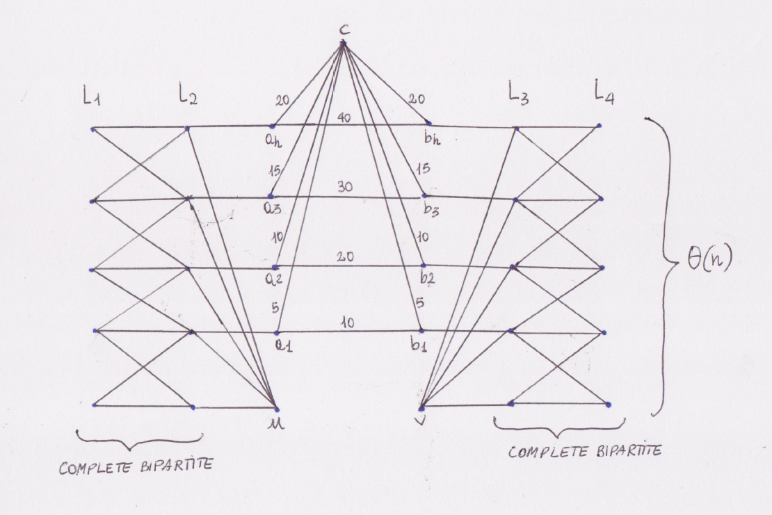
Figure 6: An example for the necessity of $CH$. The graph is oriented from left to right. Edges have unitary weight unless specified.

Appendix B Correctness of fully-dynamic

In this section, we establish the correctness of Algorithm 3 and 4.

We assume that all the local structures are correct before the update, and we will show the correctness of them after the update. fully-cleanup works with a heap $H_{c}$ of triples. The algorithm maintains the loop invariant that any triple inserted into $H_{c}$ has already been deleted from the tuple system: only its extensions remain to be processed and deleted. We prove the following lemma:

Lemma 15.

After Algorithm 3 (fully-cleanup) is executed, for any $(x,y)\in V$, the STs in $P^{*}(x,y)$ (LSTs in $P(x,y)$) represent all the SPs (LSPs) from $x$ to $y$ in $G$ that do not pass through $v$. Moreover, every THT (TLHT) present in the tuple system represents a collection of HPs (LHPs) in $G$ that contains only paths that do not pass through $v$. Finally, the sets $L,L^{*},R,R^{*}$ are correctly maintained.

Proof.

The lemma is established with the following loop invariant.

Loop Invariant: At the start of each iteration of the while loop in Step 3 of Algorithm 3 the following properties hold about the tuple system and $H_{c}$. Assume that the first triple to be extracted from $H_{c}$ and processed has min-key = $[wt,x,y]$.

1. Any LHP going through the update node $v$, which is contained in a triple $\gamma$ already processed, is removed from the tuple system. For any $a,b\in V$, if $G$ contains $c_{ab}$ LHPs of weight ${wt}$ of the form $(xa,by)$ passing through $v$, then $H_{c}$ contains a triple $\gamma=((xa,by),{wt},c_{ab})$ with key $[wt,x,y]$ already processed: the $c_{ab}$ LHPs through $v$ are cleaned from the system.

2. For each triple $\gamma=((xa,by),wt,count)$ already processed by the algorithm, $\gamma$ represents the exact set of LHPs of the form $x\rightarrow a\rightsquigarrow b\rightarrow y$ of weight $wt$ which avoid $v$. Moreover if $count=0$ the triple $\gamma$ is correctly removed from all the data structures in the tuple system associated to it. Finally, $\gamma$ has been placed in $H_{c}$ for future extensions.

   Let $[\hat{wt},\hat{x},\hat{y}]$ be the last key extracted from $H_{c}$ and processed before $[wt,x,y]$. For any key $[wt_{1},x_{1},y_{1}]\leq[\hat{wt},\hat{x},\hat{y}]$, let $G$ contain ${c}>0$ number of LHPs of weight ${wt_{1}}$ of the form $(x_{1}\times,b_{1}y_{1})$. Further, let ${c_{v}}$ (resp. ${c_{\bar{v}}}$) denote the number of such LHPs that pass through $v$ (resp. do not pass through $v$). Here ${c_{v}+c_{\bar{v}}=c}$. For every extension $(x^{\prime},wt^{\prime})\in L(x_{1},b_{1}y_{1})$, let let $wt^{\prime}=wt_{1}+{\bf{w}}(x^{\prime},x_{1})$ be the weight of the extended triple $(x^{\prime}x_{1},b_{1}y_{1})$. Then, (the following assertions are similar for $(y^{\prime},wt^{\prime})\in R(x_{1}a_{1},y_{1})$)

   1. if $c>c_{v}$ there is a triple in $P(x^{\prime},y_{1})$ of the form $(x^{\prime}x_{1},b_{1}y_{1})$ and weight $wt^{\prime}$ representing $c-c_{v}$ LHPs. If $c=c_{v}$ there is no such triple in $P(x^{\prime},y_{1})$.

   2. If a triple of the form $(x^{\prime}x_{1},b_{1}y_{1})$ and weight $wt^{\prime}$ is present as an HT in $P^{*}(x^{\prime},y_{1})$, then it represents the exact same number of LHPs $c-c_{v}$ of the corresponding triple in $P(x^{\prime},y_{1})$. This is exactly the number of HPs of the form $(x^{\prime}x_{1},b_{1}y_{1})$ and weight $wt^{\prime}$ in $G-\{v\}$.

   3. $(x^{\prime},wt^{\prime})\in L(x_{1},b_{1}y_{1})$, $(y_{1},wt^{\prime})\in R(x^{\prime}x_{1},b_{1})$ and $(x^{\prime}x_{1},b_{1}y_{1})\in$ Marked-Tuples iff ${{c_{\bar{v}}}>0}$. If the triple $(x^{\prime}x_{1},b_{1}y_{1})$ is an HT, a similar statement holds for $(x^{\prime},wt^{\prime})\in L^{*}(x_{1},y_{1})$ iff there is a triple of weight $wt_{1}$ in $P^{*}(x_{1},y_{1})$, and $(y_{1},wt^{\prime})\in R^{*}(x^{\prime},b_{1})$ iff there is a triple of weight $wt^{\prime}-{\bf{w}}(b_{1},y_{1})$ in $P^{*}(x^{\prime},b_{1})$.

   4. A triple corresponding to $(x^{\prime}x_{1},b_{1}y_{1})$ with weight $wt^{\prime}$ and counts $c_{v}$ is in $H_{c}$. A similar assertion holds for $y^{\prime}\in R(x_{1}a_{1},y_{1})$.

3. Any triple $\gamma$ in $H_{c}$, which is longer than the last triple processed, is also in Marked-Tuples if and only if it contains at least one path not passing through $v$. For any key $[wt_{2},x_{2},y_{2}]\geq[wt,x,y]$, let $G$ contain $c>0$ LHPs of weight ${wt_{2}}$ of the form $(x_{2}a_{2},b_{2}y_{2})$. Further, let ${c_{v}}$ (resp. ${c_{\bar{v}}}$) denote the number of such LHPs that pass through $v$ (resp. do not pass through $v$). Here ${c_{v}+c_{\bar{v}}=c}$. Then the tuple $(x_{2}a_{2},b_{2}y_{2})\in$ Marked-Tuples, iff $c_{\bar{v}}>0$ and a triple for $(x_{2}a_{2},b_{2}y_{2})$ is present in $H_{c}$

Initialization: We start by showing that the invariants hold before the first loop iteration. The min-key triple in $H_{c}$ has key $[0,v,v]$. Invariant assertion 1 holds since we inserted into $H_{c}$ the trivial triple of weight $0$ corresponding to the vertex $v$ and that is the only triple of such key. Moreover, since we do not represent trivial paths containing the single vertex, no counts need to be decremented. Since we assume positive edge weights, there are no LHPs in $G$ of weight less than zero. Thus all the points of invariant assertion 2 hold trivially. Invariant assertion 3 holds since $H_{c}$ does not contain any triple of weight $>0$ and we initialized Marked-Tuples to empty.

Maintenance: Assume that the invariants are true before an iteration $k$ of the loop. We prove that the invariant assertions remains true before the next iteration $k+1$. Let the min-key triple at the beginning of the $k$-th iteration be $[wt_{k},x_{k},y_{k}]$. By invariant assertion 1, we know that for any $a_{i},b_{j}$, if there exists a triple $\gamma$ of the form $(x_{k}a_{i},b_{j}y_{k})$ of weight $wt_{k}$ representing $count$ paths going through $v$, then it is present in $H_{c}$. Now consider the set of triples with key $[wt_{k},x_{k},y_{k}]$ which we extract in the set $S$ (Step 3, Algorithm 3). We consider left-extensions of triples in $S$; symmetric arguments apply for right-extensions. Consider for a particular $b$, the set $S_{b}\subseteq S$ of triples of the form $(x_{k}\times,by_{k})$ and let $fcount^{\prime}$ denote the sum of the counts of the paths represented by triples in $S_{b}$. Let $(x^{\prime},wt^{\prime})\in L(x_{k},by_{k})$ be a left extension; our goal is to generate the triple $(x^{\prime}x_{k},by_{k})$ with count $fcount^{\prime}$ and weight $wt^{\prime}=wt_{k}+{\bf{w}}(x^{\prime},x_{k})$. However, we generate such triple only if it has not been generated by a right-extension of another set of paths. We observe that the paths of the form $(x^{\prime}x_{k},by_{k})$ can be generated by right extending to $y_{k}$ the set of triples of the form $(x^{\prime}x_{k},\times b)$. Without loss of generality assume that the triples of the form $(x^{\prime}x_{k},\times b)$ have a key which is greater than the key $[wt_{k},x_{k},y_{k}]$. Thus, at the beginning of the $k$-th iteration, by invariant assertion 3, we know that $(x^{\prime}x_{k},by_{k})\notin$ Marked-Tuples. Steps 3–3, Algorithm 3 create a triple of the form $(x^{\prime}x_{k},by_{k})$ of weight $wt^{\prime}$. The generated triple can be an LST or a TLHT in $P$. In both cases the condition at step 3, Algorithm 3 holds and we remove $\gamma^{\prime}$ by decrementing $fcount^{\prime}$ many paths from the appropriate triple in $P(x^{\prime},y_{k})$. Moreover, if the generated triple is also contained in $P^{*}(x^{\prime},y_{k})$, we check if it is an ST or a THT using step 3, Algorithm 3. In the case of an ST we normally decrement $fcount^{\prime}$ paths from the appropriate triple in $P^{*}(x^{\prime},y_{k})$, otherwise we decrement the THT from $P^{*}(x^{\prime},y_{k})$ in step 3, Algorithm 3 removing only the paths going through the updated node $v$ that are contained in the THT, by using the new data structure $CH$. This establishes invariant assertions 2a and 2b. In addition, if there are no LSPs in $G$ of the form $(x^{\prime}x_{k},by_{k})$ which do not pass through $v$, we delete $(x^{\prime},wt^{\prime})$ from $L(x_{k},by_{k})$ and delete $(y_{k},wt^{\prime})$ from $R(x^{\prime}x_{k},b)$ (Step 3, Algorithm 3). On the other hand, if there exist LSPs in $G$ of the form $(x^{\prime}x_{k},by_{k})$, then $x^{\prime}$ (resp. $y_{k}$) continues to exist in $L(x_{k},by_{k})$ (resp. in $R(x^{\prime}x_{k},b)$). Further, we add the tuple $(x^{\prime}x_{k},by_{k})$ to Marked-Tuples and observe that the corresponding triple is already present in $H_{c}$ (Step 3, Algorithm 3). Similarly, if the generated triple $(x^{\prime}x_{k},by_{k})$ is an HT, then we check if $P^{*}(x_{k},y_{k})$ does not contain any triple of weight $wt_{k}$, and similarly $P^{*}(x^{\prime},b)$ does not contain any triple of weight $wt^{\prime}-{\bf{w}}(b,y_{k})$, in order to delete $(x^{\prime},wt^{\prime})$ from $L^{*}(x_{k},y_{k})$ and $(y_{k},wt^{\prime})$ from $R^{*}(x^{\prime},b)$. By the loop invariant, invariant assertions 2c and 2d were true for every key $<[wt_{k},x_{k},y_{k}]$ and by the above steps we ensure that these invariant assertions hold for every key = $[wt_{k},x_{k},y_{k}]$. Thus, invariant assertions 2c and 2d are true at the beginning of the $(k+1)$-th iteration. Note that any triple that is generated by a left extension (or symmetrically right extension) is inserted into $H_{c}$ as well as into Marked-Tuples. This establishes invariant assertion 3 at the beginning of the $(k+1)$-th iteration.

Finally, to see that invariant assertion 1 holds at the beginning of the $(k+1)$-th iteration, let the min-key at the $(k+1)$-th iteration be $[wt_{k+1},x_{k+1},y_{k+1}]$. Observe that triples with weight $wt_{k+1}$ starting with $x_{k+1}$ and ending in $y_{k+1}$ can be created either by left extending or right extending the triples of smaller weight. And since for each of iteration $\leq k$, invariant assertion 2 holds for any extension, we conclude that invariant assertion 1 holds at the beginning of the $(k+1)$-th iteration. This finishes our maintenance step.

Termination: The condition to exit the loop is $H_{c}=\emptyset$. Because invariant assertion 1 maintains in $H_{c}$ all the triples already processed, then $H_{c}=\emptyset$ implies that there are no other triples to extend in the graph $G$ that contain the updated node $v$. Moreover, because of invariant assertion 1, every triple containing the node $v$ inserted into $H_{c}=\emptyset$, has been correctly decremented from the tuple system. Finally, for invariant assertion 2c, the stacks $L,L^{*},R,R^{*}$ are correctly maintained. This completes the proof. ∎

For fully-fixup , we first show that Algorithm 4 computes the correct distances for all the SPs in the updated graph $G^{\prime}$ (Lemma 16). Moreover, we process all the new SPs in $G^{\prime}$ (Lemma 17). Finally, we show that data structures and counts are correctly maintained after the algorithm (Lemma 18). Here we use the notion of a fresh LHT for a triple that represents at least one path that is in $P$ but not in $P^{*}$. We will consider fresh triples in Lemma 17 and Observation 2.

Invariant 1.

During the execution of Algorithm 4, for any pair $(x,y)$, consider the first extraction from $H_{f}$ of a set of triples from $x$ to $y$, and let their weight be $wt$. Then $wt$ is the shortest path distance from $x$ to $y$ in the updated graph $G^{\prime}$.

Lemma 16.

Algorithm 4 maintains Invariant 1.

Proof.

Suppose for a contradiction that the invariant is violated at some extraction. Consider the earliest event in which the first set of triples $S^{\prime}$ of weight $\hat{wt}$, extracted for some pair $(x,y)$, does not contain STs in $G^{\prime}$. Let $\gamma=((xa,by),wt,count)$ be a triple in $G^{\prime}$ that represents at least one shortest path from $x$ to $y$ in $G^{\prime}$, with $wt<\hat{wt}$. The triple cannot be in $P(x,y)$ at the beginning of fixup otherwise it (or another triple with same weight $wt$) would have been inserted in $H_{f}$ during step 4 of Algorithm 4. Moreover, $\gamma$ cannot be in $H_{f}$ otherwise it would have been extracted before any triple of weight $\hat{wt}$ in $S^{\prime}$; hence $\gamma$ must be a new LST generated by the algorithm. Since all the edges incident to $v$ are added to $H_{f}$ during step 4 of Algorithm 4, then $\gamma$ must represent SPs of at least two edges. We define $left(\gamma)$ as the set of LSTs of the form $((xa,c_{i}b),wt-{\bf{w}}(b,y),count_{c_{i}})$ that represent all the LSPs in the left tuple $((xa,b),wt-{\bf{w}}(b,y))$; similarly we define $right(\gamma)$ as the set of LSTs of the form $((ad_{j},by),wt-{\bf{w}}(x,a),count_{d_{j}})$ that represent all the LSPs in the right tuple $((a,by),wt-{\bf{w}}(x,a))$.

Observe that since $\gamma$ is an ST, all the LSTs in $left(\gamma)$ and $right(\gamma)$ are also STs. A triple in $left(\gamma)$ and a triple in $right(\gamma)$ cannot be present in $P^{*}$ together at the beginning of fixup. In fact, if at least one triple from both sets is present in $P^{*}$ at the beginning of fixup, then the last one inserted during the fixup triggered by the previous update, would have generated an LST of the form $((xa,by),wt)$ automatically inserted and thus present in $P$ at the beginning of fixup (a contradiction). Thus either there is no triple in $left(\gamma)$ in $P^{*}$, or there is no triple in $right(\gamma)$ in $P^{*}$.

Assume w.l.o.g. that no triple in $right(\gamma)$ is in $P^{*}$. Since edge weights are positive, $wt-{\bf{w}}(x,a)<wt<\hat{wt}$, and because all the extractions before $\gamma$ were correct, then the triples in $right(\gamma)$ were correctly extracted from $H_{f}$ and placed in $P^{*}$ before the wrong extractions in $S^{\prime}$. If at least one triple in $left(\gamma)$ is in $P^{*}$ then the fixup would generate the tuple $((xa,by),wt)$ and place it in $P$ and $H_{f}$ (Steps 4–4, Algorithm 4). Otherwise, since $wt-{\bf{w}}(b,y)<wt<\hat{wt}$, the triples in $left(\gamma)$ were discovered by the algorithm before the wrong extractions in $S^{\prime}$. Moreover the algorithm would generate the tuple $((xa,by),wt)$ (as right extensions) and place it in $P$ and $H_{f}$ (because at least one triple in $right(\gamma)$ is already in $P^{*}$). Thus, in both cases, a tuple $((xa,by),wt)$ should have been extracted from $H_{f}$ before any triple in $S^{\prime}$. A contradiction. ∎

Invariant 2.

The set $S$ of triples constructed in Steps 4–4 of Algorithm 4 represents all the new shortest paths from $x$ to $y$.

Lemma 17.

Algorithm 4 maintains Invariant 2.

Proof.

Any new SP from $x$ to $y$ is of the following three types:

1. a single edge containing the vertex $v$ (such a path is added to $P(x,y)$ and $H_{f}$ in Step 4)

2. a path generated via left/right extension of some shortest path previously extracted from $H_{f}$ during the execution of Algorithm 4 (this generated path is added to $P(x,y)$ and $H_{f}$ in Step 4 and an analogous step in right-extend).

3. a path that was an LSP but not an SP before the update and is an SP after the update.

In type (1) and (2) above any new SP from $x$ to $y$ which is added to $H_{f}$ is also added to $P^{*}(x,y)$. However, amongst the several triples representing paths of the type (3) listed above, only one candidate triple will be present in $H_{f}$. Thus we conclude that, for a given $x,y$, when we extract from $H_{f}$ a type (3) triple of weight $wt$, $P(x,y)$ could contain a superset of triples with the same weight $wt$ that are not present in $H_{f}$. We now consider the two cases the algorithm deals with.

• $P^{*}(x,y)$ increased its min-weight, when the first set of triples for $x,y$ is extracted from $H_{f}$. This is the only case where we could restore historical triples, or process fresh triples from scratch because they are not yet in $P^{*}$ or they are present in $P^{*}$ with a lower count than the corresponding triple in $P$ (note that this condition is triggered only by increase-only updates). To do that we process all the min-weight triples in $P(x,y)$, but before we really add a triple in $S$ for further extensions, we check if it is present in $P^{*}$ with a lower count (Step 4, Algorithm 4), or it is not present in $P^{*}$ (Step 4, Algorithm 4). By the above argument, we consider all the new STs from $x$ to $y$ present in $P(x,y)$. Therefore it suffices to argue that all of them contains new shortest paths to be processed. Suppose for contradiction that some triple $\gamma$ does not contains new shortest paths. Thus, $\gamma$ was a ST before the update and already in $P^{*}$ with at least one path not going through $v$. However, since cleanup only removes paths that contain $v$, the triple $\gamma$ remained in $P^{*}(x,y)$ after the fully-cleanup phase. This contradicts the fact that $P^{*}(x,y)$ increased its min-weight.

• $P^{*}(x,y)$ didn’t change its min-weight when the first set of triples for $x,y$ is extracted from $H_{f}$. Let the weight of triples in $P^{*}(x,y)$ be $wt$. This implies that the shortest path distance from $x$ to $y$ before and after the update is $wt$. Both in the case of decrease-only and increase-only updates, all the new paths that we need to consider from $x$ to $y$ are going through the updated node $v$. By construction of the Algorithm 4, every triple containing the updated node $v$ is always placed into $H_{f}$. Thus it suffices to consider only triples in $H_{f}$.

∎

Observation 2.

During the execution of Algorithm 4, consider a THT $\tau$ that becomes shortest. If $\tau$’s corresponding triple in $P$ is not fresh, then it is simply restored (not processed); otherwise $\tau$’s count is replaced with the updated count from $P$ and it is extended anew.

Proof.

When we restore an existing HT $\tau$ from $P^{*}$, we always check if its corresponding triple in $P$ contains more paths (Step 4, Algorithm 4) or the counts match. In the first case $\tau$ in $P^{*}$ is carrying an obsolete number of SPs and is therefore replaced with the correct count in $P$ and extended anew (Step 4, Algorithm 4). Otherwise it is still representing the correct number of SPs to be restored and it is not processed. ∎

Lemma 18.

After the execution of Algorithm 4 (fully-fixup), for any $(x,y)\in V$, the STs in $P^{*}(x,y)$ (LSTs in $P(x,y)$) represent all the SPs (LSPs) from $x$ to $y$ in the updated graph. Also, the sets $L,L^{*},R,R^{*}$ are correctly maintained.

Proof.

Loop Invariant: At the start of each iteration of the while loop in Step 4 of Algorithm 4, assume that the first triple in $H_{f}$ to be extracted and processed has min-key = $[wt,x,y]$. Then the following properties hold about the tuple system and $H_{f}$.

1. If $G$ contains $c_{ab}$ SPs of form $(xa,by)$ and weight ${wt}$, then $H_{f}$ contains a triple of form $(xa,by)$ and weight $wt$ to be extracted and processed. For any $a,b\in V$, if $G^{\prime}$ contains $c_{ab}$ SPs of form $(xa,by)$ and weight ${wt}$, then $H_{f}$ contains a triple of form $(xa,by)$ and weight $wt$ to be extracted and processed. Further, a triple $\gamma=((xa,by),{wt},c_{ab})$ is present in $P(x,y)$.

2. Let $[\hat{wt},\hat{x},\hat{y}]$ be the last key extracted from $H_{f}$ and processed before $[wt,x,y]$. Every SP in $G$, with an associated key $[wt_{1},x_{1},y_{1}]\leq[\hat{wt},\hat{x},\hat{y}]$, is represented by a triple $\gamma$ in the tuple system having the correct count. Moreover, the tuple system contains all the valid extensions derived by $\gamma$, and any extension of $\gamma$ itself is present in $H_{f}$ as a candidate triple. For any key $[wt_{1},x_{1},y_{1}]\leq[\hat{wt},\hat{x},\hat{y}]$, let $G^{\prime}$ contain ${c}>0$ number of LHPs of weight ${wt_{1}}$ of the form $(x_{1}a_{1},b_{1}y_{1})$. Further, let ${c_{new}}$ (resp. ${c_{old}}$) denote the number of these LHPs that are new (resp. not new). Here ${c_{new}+c_{old}=c}$. If $c_{new}>0$ then,

   1. there is an LHT in $P(x_{1},y_{1})$ of the form $(x_{1}a_{1},b_{1}y_{1})$ and weight $wt_{1}$ that represents $c$ LHPs.

   2. If a triple of the form $(x_{1}a_{1},b_{1}y_{1})$ and weight $wt_{1}$ is present as an HT in $P^{*}$, then it represents the exact same count of $c$ HPs of its corresponding triple in $P$. This is exactly the number of HPs of the form $(x_{1}a_{1},b_{1}y_{1})$ and weight $wt_{1}$ in $G^{\prime}$.

   3. $(x_{1},wt_{1})\in L(a_{1},b_{1}y_{1})$, $(y_{1},wt_{1})\in R(x_{1}a_{1},b_{1})$, and if the triple of the form $(x_{1}a_{1},b_{1}y_{1})$ and weight $wt_{1}$ is also shortest then $(x_{1},wt_{1})\in L^{*}(a_{1},y_{1})$, $(y_{1},wt_{1})\in R^{*}(x_{1},b_{1})$. Further, $(x_{1}a_{1},b_{1}y_{1})\in$ Marked-Tuples iff ${{c_{old}}>0}$.

   4. If $c_{new}>0$, for every $(x^{\prime},wt^{\prime})\in L(x_{1},b_{1}y_{1})$, an LHT corresponding to $(x^{\prime}x_{1},b_{1}y_{1})$ with weight $wt^{\prime}~{}=~{}wt_{1}~{}+~{}{\bf{w}}(x^{\prime},x_{1})\geq wt$ and counts equal to the sum of new paths represented by its constituents, is in $H_{f}$ and $P$. A similar assertion holds for $(y^{\prime},wt^{\prime})\in R(x_{1}a_{1},y_{1})$.

3. Any triple $\gamma$ in $H_{f}$, which is longer than the last triple processed, is also in Marked-Tuples if and only if it contains at least one old LHP (generated by a previous update) and a new LHP added to $H_{f}$ during a previous step of the current update. For any key $[wt_{2},x_{2},y_{2}]\geq[wt,x,y]$, let $G^{\prime}$ contain $c>0$ number of LHPs of weight ${wt_{2}}$ of the form $(x_{2}a_{2},b_{2}y_{2})$. Further, let ${c_{new}}$ (resp. ${c_{old}}$) denote the number of such LHPs that are new (resp. not new). Here ${c_{new}+c_{old}=c}$. Then the tuple $(x_{2}a_{2},b_{2}y_{2})\in$ Marked-Tuples, iff $c_{old}>0$ and $c_{new}$ paths have been added to $H_{f}$ by some earlier iteration of the while loop.

Initialization and Maintenance for the 3 invariant assertions are similar to the proof of Lemma 15.

Termination: The condition to exit the loop is $H_{f}=\emptyset$. Because invariant assertion 1 maintains in $H_{f}$ the first triple to be extracted and processed, then $H_{f}=\emptyset$ implies that there are no triples, formed by a valid left or right extensions, that contain new SPs or LSPs, that need to be added or restored in the graph $G$. Moreover, because of invariant assertions 2a and 2b, every triple containing the node $v$, extracted and processed before $H_{f}=\emptyset$, has been added or restored with its correct count in the tuple system. Finally, for invariant assertion 2c, the stacks $L,L^{*},R,R^{*}$ are correctly maintained. This completes the proof of the loop invariant.

By Lemma 17, all the new SPs in $G^{\prime}$ are placed in $H_{f}$ and processed by the algorithm and hence are in $P^{*}$ after the execution of Algorithm 4. Moreover, for a pair $(x,y)$, the check in Step 4 of Algorithm 4 would fail if the distance from $x$ to $y$ doesn’t change after the update. Thus the old SPs from $x$ to $y$ will remain in $P^{*}(x,y)$. Hence, after Algorithm 4 is executed, every SP in $G^{\prime}$ is in its corresponding $P^{*}$.

Since every LST of the form $(xa,by)$ in $G^{\prime}$ is formed by a left extension of a set of STs of the form $(a\times,by)$ (Steps 4–4, Algorithm 4), or a right extension of a set of the form $(xa,\times b)$ (analogous steps for right extensions), and all the STs are correctly maintained by the algorithm, then all the LSTs are correctly maintained at the end of the fixup algorithm. This completes the proof of the Lemma. ∎

Appendix C The ffd Algorithm for APASP

C.1 Description of ff-cleanup

ff-cleanup removes all the LHPs going through the updated vertex $v$ from all the global structures $P$, $P^{*}$, $L$ and $R$, and from all local structures in any active level graph $\Gamma_{j}$ that contains these triples. This involves decrementing the count of some triples or removing them completely (when all the paths in the triple go through $v$). The algorithm also updates local dictionaries and the $DL$, $RN$ and $LN$ structures. Algorithm ff-cleanup is a natural extension of the NPRdec cleanup. An extension of the NPRdec cleanup is used also in our basic algorithm but in a different way.

1$H_{c}\leftarrow\emptyset$; Marked-Tuples $\leftarrow\emptyset$;

2 $\gamma\leftarrow[(v,v),0,1]$; $C_{\gamma}[center(v)]=1$; add $[\gamma,C_{\gamma}]$ to $H_{c}$;

3 while $H_{c}\neq\emptyset$  do

4       extract in $S$ all the triples with the same min-key $[wt,x,y]$ from $H_{c}$;

5       ff-cleanup-$\ell$-extend($S$,$[wt,x,y]$) (see Algorithm 9);

6       ff-cleanup-$r$-extend($S$,$[wt,x,y]$);

7      

Algorithm 8 ff-cleanup$(v)$

ff-cleanup starts as in the NPRdec algorithm. We add the updated node $v$ to $H_{c}$ (Step 8 – Alg. 8) and we start extracting all the triples with same min-key (Step 8 – Alg. 8). The main differences from NPRdec start after we call Algorithm 9. As in [21], we start by forming a new triple $\gamma^{\prime}$ to be deleted (Steps 9 – Alg. 8). A new feature in Algorithm 9 is to accumulate the paths that we need to remove level by level using the array $C^{\prime}$. This is inspired by Thorup where unique SPs are maintained in each level. However, our algorithm maintains multiples paths spread across different levels using the $C_{\gamma}$ arrays associated to LSTs, and the technique used to update the $C_{\gamma}$ arrays is significantly different and more involved than the one described in Thorup. Step 9 - Alg. 9 calls ff-cleanup-centers (Alg. 10) that will perform this task.

1for every $b$ such that $(x\times,by)\in S$ do

2       let $S_{b}\subseteq S$ be the set of all triples of the form $(x\times,by)$;

3       let $fcount^{\prime}$ be the sum of all the $counts$ of all triples in $S_{b}$;

4       for every $x^{\prime}$ in $L(x,by)$ s.t. $(x^{\prime}x,by)\notin$ Marked-Tuples  do

5             $wt^{\prime}\leftarrow wt+{\bf{w}}(x^{\prime},x)$; $\gamma^{\prime}\leftarrow((x^{\prime}x,by),wt^{\prime},fcount^{\prime})$;

6             $C_{\gamma^{\prime}}\leftarrow$ ff-cleanup-centers$(\gamma^{\prime},S_{b})$;

7             add $[\gamma^{\prime},C_{\gamma^{\prime}}]$ to $H_{c}$;

8             remove $\gamma^{\prime}$ in $P(x^{\prime},y)$ // decrements $count$ by $fcount^{\prime}$;

9             set new center for $\gamma^{\prime\prime}=((x^{\prime}x,by),wt^{\prime})$ in $P(x^{\prime},y)$ as $\arg\!\min_{i}(C_{\gamma^{\prime\prime}}[i]\neq 0)$;

10             if  a triple for $(x^{\prime}x,by)$ exists in $P(x^{\prime},y)$ then

11                   insert $(x^{\prime}x,by)$ in Marked-Tuples;

12                  

13            else

14                   delete $x^{\prime}$ from $L(x,by)$ and delete $y$ from $R(x^{\prime}x,b)$;

15                  

16             if  no triple for $((x^{\prime}-,by),wt^{\prime})$ exists in $P(x^{\prime},y)$ then

17                   remove $b$ from $RN(x^{\prime},y,wt^{\prime})$;

18                  

19            if  no triple for $((x^{\prime}x,-y),wt^{\prime})$ exists in $P(x^{\prime},y)$ then

20                   remove $x$ from $LN(x^{\prime},y,wt^{\prime})$;

21                  

22             if a triple for $((x^{\prime}x,by),wt^{\prime})$ exists in $P^{*}(x^{\prime},y)$ then

23                   remove $\gamma^{\prime}$ in $P^{*}(x^{\prime},y)$ // decrements $count$ by $fcount^{\prime}$;

24                   if $\gamma^{\prime}\notin P^{*}(x^{\prime},y)$ then

25                         remove the element with weight $wt^{\prime}$ from $DL(x^{\prime},y)$ if not linked to other tuples in $P^{*}(x^{\prime},y)$;

26                        

27                  for each $i$ do

28                         decrement $C_{\gamma^{\prime}}[i]$ paths from $\gamma^{\prime}\in P^{*}_{i}(x^{\prime},y)$;

29                         if $\gamma^{\prime}$ is removed from $P^{*}_{i}(x^{\prime},y)$ then

30                               if $x^{\prime}$ is centered in level $i$ then

31                                     if $\forall\,j\geq i,P^{*}_{j}(x,y)=\emptyset$ or $x^{\prime}=v$ then

32                                           remove $x^{\prime}$ from $L^{*}_{i}(x,y)$ and remove $x^{\prime}$ from $LC^{*}_{i}(x,y)$;

33                                          

34                               else if $P^{*}_{i}(x,y)=\emptyset$ or $x^{\prime}=v$ then

35                                     remove $x^{\prime}$ from $L^{*}_{i}(x,y)$;

36                                    

37                               if $y$ is centered in level $i$ then

38                                     if $\forall\,j\geq i,P^{*}_{j}(x^{\prime},b)=\emptyset$ or $y=v$ then

39                                           remove $y$ from $R^{*}_{i}(x^{\prime},b)$ and remove $y$ from $RC^{*}_{i}(x^{\prime},b)$;

40                                          

41                               else if $P^{*}_{i}(x^{\prime},b)=\emptyset$ or $y=v$ then

42                                     remove $y$ from $R^{*}_{i}(x^{\prime},b)$;

43                                    

44                              

45                        

Algorithm 9 ff-cleanup-$\ell$-extend($S,[wt,x,y]$)

1let $\gamma^{\prime}=((x^{\prime}x,by),wt^{\prime},fcount^{\prime})$ (the triple of the form $((x^{\prime}x,by),wt^{\prime})$ that contains all the paths through $v$ to be removed);

2 let $\gamma^{\prime\prime}=((x^{\prime}x,by),wt^{\prime},fcount^{\prime\prime})$ (the triple of the form $((x^{\prime}x,by),wt^{\prime})$ in $P(x^{\prime},y)$. Note that $\gamma^{\prime}$ represents a subset of $\gamma^{\prime\prime}$);

3 $j\leftarrow\arg\!\max_{j}(C_{\gamma^{\prime\prime}}[j]\neq 0)$ // This is the oldest level in which a path in $\gamma^{\prime\prime}$ appeared for the first time;

4 $C^{\prime}\leftarrow\sum_{\gamma\in S_{b}}{C_{\gamma}[r-1,\ldots,0]}$ // This is the sum (level by level) of the triples of the form $(xa_{i},by)$ that go through $v$ and are extending to $\gamma^{\prime}$ during this stage;

5 create a new center vector $C_{\gamma^{\prime}}$ for the triple $\gamma^{\prime}$ as follows;

6         for all the levels $m>j$ we set $C_{\gamma^{\prime}}[m]=0$;

7         for the level $j$ we set $C_{\gamma^{\prime}}[j]=\sum_{k=j}^{r-1}{C^{\prime}[k]}$;

8         for all the levels $i<j$ we set $C_{\gamma^{\prime}}[i]=C^{\prime}[i]$;

9 $C_{\gamma^{\prime\prime}}[r-1,\ldots,0]\leftarrow C_{\gamma^{\prime\prime}}[r-1,\ldots,0]-C_{\gamma^{\prime}}[r-1,\ldots,0]$ // We update the $C$ vector for $\gamma^{\prime\prime}\in P(x^{\prime},y)$;

10 return $C_{\gamma^{\prime}}$ // We return the correct vector for the generated $\gamma^{\prime}$ triples;

Algorithm 10 ff-cleanup-centers$(\gamma^{\prime},S_{b})$

ff-cleanup-centers takes as input the generated triple $\gamma^{\prime}$ of the form $(x^{\prime}x,by)$ which contains all the paths going through the updated node $v$ to be removed, and the set of triples $S_{b}$ of the form $(x\times,by)$ that are extended to $x^{\prime}$ to generate $\gamma^{\prime}$. This procedure has two tasks: (1) generating the $C_{\gamma^{\prime}}$ vector for the triple $\gamma^{\prime}$ that will be reinserted in $H_{c}$ for further extensions, and (2) updating the $C_{\gamma^{\prime\prime}}$ vector for the tuple $\gamma^{\prime\prime}$ in $P(x^{\prime},y)$ (note that $\gamma^{\prime\prime}$ is the corresponding triple in $P$ of $\gamma^{\prime}$, before we subtract all the paths represented by $\gamma^{\prime}$ level by level).
(1) - This task, which is more complex than the second task (which is a single step in the algorithm, see point (2) below), is accomplished in steps 10 to 10, Alg. 10 and uses the following technique. In step 10 – Alg. 10, we store into the $\log n$-size array $C^{\prime}$ the distribution over the active levels for the set of triples in $S_{b}$ that generates $\gamma^{\prime}$ using the left extension to $x^{\prime}$. In order to generate the correct vector $C_{\gamma^{\prime}}$ (to associate with the triple $\gamma^{\prime}$), we need to reshape the distribution in $C^{\prime}$ according to the corresponding distribution of the triple $\gamma^{\prime\prime}\in P$. The reshaping procedure works as follows: we first identify the oldest level $j$ in which the triple $\gamma^{\prime\prime}$ appeared in $P$ for the first time (Step 10 – Alg. 10). Recall that we want to remove $\gamma^{\prime}$ paths containing $v$ from $\gamma^{\prime\prime}$, and $\gamma^{\prime\prime}$ does not exist in any level older than $j$. Vector $C^{\prime}$ is the sum of $C_{\gamma}$ for all $\gamma\in S_{b}$ (Step 10 – Alg. 10). Those triples are of the form $(xa_{i},by)$ and they could exist in levels older, equal or more recent than $j$. But the triples in $S_{b}$ that were present in a level older than $j$, were extended to $\gamma^{\prime\prime}$ in $P$ for the first time in level $j$. For this reason, step 10 - Alg. 10 aggregates all the counts in $C^{\prime}$ in levels older or equal $j$ in $C_{\gamma^{\prime}}[j]$. Moreover, for each level $i<j$, if a triple $\gamma\in S_{b}$ is present in the level graph $\Gamma_{i}$ with $count$ paths centered in level $i$, then $\Gamma_{i}$ also contains its extension to $x^{\prime}$ that is a subtriple of $\gamma^{\prime\prime}$ located in level $i$ with at least $count$ paths. Thus for each level $i<j$ step 10 - Alg. 10, copies the number of paths level-wise. This procedure allows us to precisely remove the LHPs only from the level graphs where they exist. After $C^{\prime}$ is reshaped into $C_{\gamma^{\prime}}$ (steps 10 to 10 - Alg. 10), the algorithm returns this correct array for $\gamma^{\prime}$ to Alg. 9.
(2) - This task is performed by the simple step 10, Alg. 10, which is a subtraction level by level of LHPs.

After adding the new triple $\gamma^{\prime}$ to $H_{c}$ (Step 9 - Alg. 9), the algorithm continues as the NPRdec (Steps 9 to 9 – Alg. 9) with some differences: we need to update centers, local data structures, $DL$, $RN$ and $LN$. We update the center of $\gamma^{\prime}$ using $C_{\gamma^{\prime}}$ (Step 9 - Alg. 9). If $\gamma^{\prime}$ is a shortest triple, we decrement the count of $\gamma^{\prime}\in P^{*}(x^{\prime},y)$ (Step 9 - Alg. 9). If $\gamma^{\prime}$ is completely removed from $P^{*}(x^{\prime},y)$ and $DL(x^{\prime},y,wt^{\prime})$ is not linked to any other tuple, we remove the entry with weight $wt^{\prime}$ from $DL(x^{\prime},y)$ (Step 9 - Alg. 9). Moreover, we subtract the correct number of paths from each level using the (previously built) array $C_{\gamma^{\prime}}$ (Step 9 - Alg. 9). Finally for each active level $i$, if $\gamma^{\prime}$ is removed from $P^{*}_{i}(x^{\prime},y)$, we take care of the sets $L_{i}^{*}$ and $R_{i}^{*}$ (Steps 9 to 9 - Alg. 9). In the process, we also update $LC_{i}^{*}$ and $RC_{i}^{*}$ in case the endpoints of $\gamma^{\prime}$ are centered in level $i$. If $\gamma^{\prime}$ is completely removed from $P(x^{\prime},y)$, using the double links to the node $b$ in $RN(x^{\prime},y,wt^{\prime})$, we check if there are other triples that use $b$ in $P(x^{\prime},y)$ (Step 9 - Alg. 9): if not we remove $b$ from $RN(x^{\prime},y,wt^{\prime})$. A similar step handles $LN(x^{\prime},y,wt^{\prime})$.

C.2 Description of ff-fixup

ff-fixup is an extension of fully-fixup rather than NPRdec. This is because of the presence of the control bit $\beta$ (defined in Section 5.2), and the need to process historical triples (that are not present in NPRdec). Algorithm ff-fixup will efficiently maintain exactly the LSTs and STs for each level graph in the tuple system. This is in contrast to fully-fixup, which can maintain LHTs that are not LSTs in any level graph (PDG). ff-fixup maintains a heap $H_{f}$ of candidate LHTs to be processed in min-weight order. The main phase (Alg. 11) is very similar to the fixup in our basic algorithm. The differences are again related to levels, centers and the new data structures.

We start describing Algorithm 11. We initialize $H_{f}$ by inserting the edges incident on the updated vertex $v$ with their updated weights (Steps 12 to 12 – Alg. 12), as well as a candidate min-weight triple from $P$ for each pair of nodes $(x,y)$ (Step 12 – Alg. 12). Then we process $H_{f}$ by repeatedly extracting collections of triples of the same min-weight for a given pair of nodes, until $H_{f}$ is empty (Steps 11 to 11 – Alg. 11). We will establish that the first set of triples for each pair $(x,y)$ always represents the shortest path distance from $x$ to $y$ (see Lemma 20), and the triple extracted are added to the tuple system if not already there (see Alg. 13 and Lemma 21). For efficiency, among all the triples present in the tuple system for a pair of nodes, we select only the ones that need to be extended: this task is performed by Algorithm 13 (this step is explained later in the description). After the triples in $S$ are left and right extended by Algorithm 14, we set the bit $\beta(\gamma^{\prime})=1$ for each triple $\gamma^{\prime}$ that is identified as shortest in $S$, since $\gamma^{\prime}$ is correctly updated both in $P^{*}(x,y)$ and $P(x,y)$ (Step 11 – Alg. 11). Finally, we update the $DL(x,y)$ structure by inserting (or updating if an element with weight $wt$ is already present) the element with weight $wt$ and the current level at the end of the list (Step 11 – Alg. 11). This concludes the description of Algorithm 11.

We now describe Algorithm 13 which is responsible to select only the triples that have valid extensions that will generate LHTs in the current graph. In Algorithm 13, we distinguish two cases. When the set of extracted triples from $x$ to $y$ contains at least one path not containing $v$ (Step 13 – Alg. 13), then we process all the triples from $P(x,y)$ of the same weight. Otherwise, if all the paths extracted go through $v$ (Step 13 – Alg. 13), we only use the triples extracted from $H_{f}$.

1$H_{f}\leftarrow\emptyset$; Marked-Tuples $\leftarrow\emptyset$;

2 ff-populate-heap$(v,{\bf{w}}^{\prime},k)$;

3 while $H_{f}\neq\emptyset$ do

4       extract in $S^{\prime}$ all the triples with min-key $[wt,x,y]$ from $H_{f}$;

5       if $S^{\prime}$ is the first extracted set from $H_{f}$ for $x,y$ then

6             $S\leftarrow$ ff-new-paths($S^{\prime},P(x,y)$);

7             ff-fixup-$\ell$-extend($S$,$[wt,x,y]$) (see Algorithm 14);

8             ff-fixup-$r$-extend($S$,$[wt,x,y]$);

9             for every $\gamma\in S$ set $\beta(\gamma)=1$;

10             add an element with weight $wt$ and level $k$ to $DL(x,y)$ or update the level in the existing one;

11            

Algorithm 11 ff-fixup$(v,{\bf{w}}^{\prime},k)$

1for each $(u,v)$ do

2       ${\bf{w}}(u,v)={\bf{w}}^{\prime}(u,v)$;

3       if ${\bf{w}}(u,v)<\infty$  then

4             $\gamma=((uv,uv),{\bf{w}}(u,v),1)$; $C_{\gamma}[k]\leftarrow 1$;

5             update-num($\gamma$) $\leftarrow$ curr-update-num; num-v-paths($\gamma$) $\leftarrow 1$;

6             add $[\gamma,C_{\gamma}]$ to $H_{f}$ and $P(u,v)$;

7             add $u$ to $L(-,vv)$ and $v$ to $R(uu,-)$;

8            

9      

10for each $(v,u)$ do

11       symmetric processing as Steps 12–12 above;

12      

13for each $x,y\in V$ do

14       add a min-key triple $[\gamma,C_{\gamma}]\in P(x,y)$ to $H_{f}$;

15      

Algorithm 12 ff-populate-heap$(v,{\bf{w}}^{\prime},k)$

1$S\leftarrow\emptyset$; let $i$ be the min-weight level associated with $DL(x,y)$;

2 if $P^{*}(x,y)$ increased min-weight after cleanup then

3       for each $\gamma^{\prime}\in S$ with-key $[wt,0]$ do

4             let $\gamma^{\prime}=((xa^{\prime},b^{\prime}y),wt,count^{\prime})$ and $j=\arg\!\min_{j}(C_{\gamma^{\prime}}[j]\neq 0)$;

5             if $\gamma^{\prime}$ is not in $P^{*}(x,y)$ then

6                   add $\gamma^{\prime}$ in $P^{*}(x,y)$ and $S$; add $x$ to $L^{*}(a^{\prime},y)$ and $y$ to $R^{*}(x,b^{\prime})$;

7                   add $b^{\prime}$ to $RN(x,y,wt)$; place a double link between $\gamma^{\prime}$ and $DL(x,y,wt)$;

8                  

9             else if $\gamma^{\prime}$ is in $P(x,y)$ and $P^{*}(x,y)$ with different counts then

10                   replace the count of $\gamma^{\prime}$ in $P^{*}(x,y)$ with $count^{\prime}$ and add $\gamma^{\prime}$ to $S$;

11                  

12             add $\gamma^{\prime}$ to $P^{*}_{j}(x,y)$ and $dict_{j}$;

13             add $x$ to $L^{*}_{j}(a^{\prime},y)$ and $y$ to $R^{*}_{j}(x,b^{\prime})$;

14             add $x$ to $LC^{*}_{j}(a^{\prime},y)$ ($y$ to $RC^{*}_{j}(x,b^{\prime})$) if $x$ ($y$) is a level $i$ center;

15             add $\gamma^{\prime}$ in $S$;

16            

17      for each $b^{\prime}\in RN(x,y,wt)$ do

18             if $\exists\,h<i:L_{h}^{*}(x,b^{\prime})\neq\emptyset$ then

19                   add any $\gamma^{\prime}$ of the form $(x\times,b^{\prime}y)$ and weight $wt$ in $P^{*}(x,y)$ with $\beta(\gamma^{\prime})=1$ to $S$;

20                  

21else

22       for each $\gamma^{\prime}\in S^{\prime}$ containing a path through $v$ do

23             let $\gamma^{\prime}=((xa^{\prime},b^{\prime}y),wt,count^{\prime})$ and $k$ the current level;

24             add $\gamma^{\prime}$ with paths$(\gamma^{\prime},v)$ to $P^{*}(x,y)$, and $[\gamma^{\prime},C_{\gamma^{\prime}}]$ to $S$;

25             add $\gamma^{\prime}$ to $P^{*}_{k}(x,y)$ and $dict_{k}$, $x$ to $L^{*}_{k}(a^{\prime},y)$ and $y$ to $R^{*}_{k}(x,b^{\prime})$;

26             add $x$ to $LC^{*}_{k}(a^{\prime},y)$ ($y$ to $RC^{*}_{k}(x,b^{\prime})$) if $x$ ($y$) is a level $k$ center;

27            

28      

29return $S$;

Algorithm 13 ff-new-paths($S^{\prime},P_{xy}$)

Both cases have a similar approach but here we focus on the former which is more involved than the latter. As soon as we identify a new triple $\gamma^{\prime}$ we compute its center $j$ by using its associated array $C_{\gamma^{\prime}}$ (Step 13 – Alg. 13). This is straightforward if compared to ff-cleanup where we first need to update the center arrays. We add this triple to $P^{*}(x,y)$ and to $S$, which contains the set of triples that need to be extended. We also add $\gamma^{\prime}$ to $P_{j}^{*}(x,y)$ (Steps 13 and 13 – Alg. 13). We update $dict_{j}$ to keep track of the locations of the triple in the global structures. A similar sequence of steps takes place when all the extracted paths go through $v$ (Steps 13 to 13 – Alg. 13). The only difference is that the local data structures to be updated are only the $\Gamma_{k}$ data stuctures (Steps 13 and 13 – Alg. 13).

A crucial difference from fully-fixup and this algorithm is the way we collect the set $S$ of triples to be extended. Here we require the new HE data structures $RN$ and $LN$ (see Section 5.2.2) because of PEP instances (see Section 5.3). Let $i$ be the min-weight level associated with $DL(x,y)$. For each node $b\in RN(x,y,wt)$ we check if $L_{h}^{*}(x,b)$ contains at least one extension, for every $h<i$ (Steps 13 to 13 – Alg. 13). In fact we need to discover all tuples with $\beta=1$ that are inside a PEP instance. In this instance, the triples restored as STs may or may not be extended. We cannot afford to look at all of them, thus our solution should check only the triples with an available extension. Moreover, all the extendable triples with with $\beta=1$ have extension only in levels younger than the level where they last appear as STs. Thus, we check for extensions only in the levels $h<i$.

Using the HE sets, is the key to avoid an otherwise long search of all the valid extensions for the set of examined triples with $\beta=1$. In particular, without the HE sets, the algorithm could waste time by searching for extensions that are not even in the tuple system. Correctness of this method is proven in section 6. After the algorithm collects the set $S$ of triples that can be extended, ff-fixup calls ff-fixup-$\ell$-extend (Alg. 14).

1for every $b$ such that $(x\times,by)\in S$ do

2       let $S_{b}\subseteq S$ be the set of all triples of the form $(x\times,by)$;

3       let $fcount^{\prime}$ be the sum of all the $counts$ of all triples in $S_{b}$; let $h$ be the $center(S_{b})$;

4       if $\exists\,\gamma\in S_{b}:\beta(\gamma)=0$ then

5             let $j$ be the level associated to the minweight $wt^{\prime}>wt$ in $DL(x,y)$;

6             for every active level $h\leq i<j$ do

7                   for every $x^{\prime}$ in $L_{i}^{*}(x,b)$ do

8                         if $(x^{\prime}x,by)\notin$ Marked-Tuples  then

9                               $wt^{\prime}\leftarrow wt+{\bf{w}}(x^{\prime},x)$; $\gamma^{\prime}\leftarrow((x^{\prime}x,by),wt^{\prime},fcount^{\prime})$;

10                               $C_{\gamma^{\prime}}\leftarrow$ ff-fixup-centers($S_{b}$); add $\gamma^{\prime}$ to $H_{f}$;

11                               if a triple $\gamma^{\prime\prime}$ for $((x^{\prime}x,by),wt^{\prime})$ exists in $P(x^{\prime},y)$ then

12                                     update the count of $\gamma^{\prime\prime}$ in $P(x^{\prime},y)$ and $C_{\gamma^{\prime\prime}}=C_{\gamma^{\prime\prime}}+C_{\gamma^{\prime}}$;

13                                     add $(x^{\prime}x,by)$ to Marked-Tuples ;

14                                    

15                              else

16                                     add $[\gamma^{\prime},C_{\gamma^{\prime}}]$ to $P(x^{\prime},y)$; add $x^{\prime}$ to $L(x,by)$ and $y$ to $R(x^{\prime}x,b)$;

17                                    

18                              set $\beta(\gamma^{\prime})=0$; set update-num($\gamma^{\prime}$);

19                              

20             for every level $i<h$ do

21                   for every $x^{\prime}$ in $LC_{i}^{*}(x,b)$ do

22                         execute steps 14 to 14;

23                        

24            

25      else

26             let $j$ be the level associated to the minweight $wt$ in $DL(x,y)$;

27             for every level $i<j$ do

28                   for every $x^{\prime}$ in $LC_{i}^{*}(x,b)$ do

29                         execute steps 14 to 14;

30                        

31            

Algorithm 14 ff-fixup-$\ell$-extend($S$,$[wt,x,y]$)

1let $C^{\prime}=\sum_{\gamma\in S_{b}}{C_{\gamma}}$ be the sum (level by level) of the new paths that are found shortest;

2 let $j$ be $\arg\!\max_{j}(C^{\prime}[j]\neq 0)$, and $k=center(x^{\prime})$;

3 if $k<j$ then

4       for all the levels $i<k$ we set $C_{\gamma^{\prime}}[i]=C^{\prime}[i]$;

5       for the level $k$ we set $C_{\gamma^{\prime}}[k]=\sum_{q=k}^{r-1}{C^{\prime}[q]}$;

6       for all the levels $m>k$ we set $C_{\gamma^{\prime}}[m]=0$;

7      

8else

9       $C_{\gamma^{\prime}}=C^{\prime}$;

10      

11return $C_{\gamma^{\prime}}$;

Algorithm 15 ff-fixup-centers$(S_{b})$

Here we describe the details of algorithm 14. Its goal is to generate LHTs for the current graph $G$ by extending HTs. Let $h$ be the center of $S_{b}$ defined as the most recent center among all the triples in $S_{b}$, and let $j$ be the level associated to the first weight $wt^{\prime}$ larger than $wt$ in $DL(x,y)$. The extension phase for triples is different from fully-fixup: in fact, the set of triples $S_{b}$ could contain only triples with $\beta(\gamma)=1$. In fully-fixup, the corresponding set $S_{b}$ contains only triples with $\beta(\gamma)=0$. We address two cases:
(a) – If $S_{b}$ contains at least one triple $\gamma$ with $\beta(\gamma)=0$, we extend $S_{b}$ using the sets $L_{i}^{*}$ and $R_{i}^{*}$ with $h\leq i<j$ (Steps 14 to 14 – Alg.14). In fact, the set $S_{b}$ contains at least one new path that was not extended in the previous iterations when $wt$ was the shortest distance from $x$ to $y$ (because of the $\beta(\gamma)=0$ triple). The LST generated in this way remains centered in level $h$. Moreover we extend $S_{b}$ also using the sets $LC_{i}^{*}$ and $RC_{i}^{*}$ with $i<h$ (Steps 14 to 14 – Alg.14). This ensures that every LST generated in a level $i$ lower than $h$ is centered in $i$ thanks to the extension node itself. This technique guarantees that each LHT generated by Algorithm 14 is an LST centered in a unique level.
(b) – In the case when there is no triple $\gamma$ in $S_{b}$ with $\beta(\gamma)=0$, then there is at least one extension to perform for $S_{b}$ and it must be in some level younger than the level where $wt$ stopped to be the shortest distance from $x$ to $y$ (this follows from the use of the HE sets in Alg. 13). To perform these extensions we set $j$ as the level associated with the min-weight element in $DL(x,y)$, and we extend $S_{b}$ using the sets $LC_{i}^{*}$ and $RC_{i}^{*}$ with $i<j$ (Steps 14 to 14 – Alg.14). Again, every LHT generated is an LST centered in a unique level. Finally, every generated LHT is added to $P$ and $H_{f}$ and we update global $L$ and $R$ structures.

Observation 3.

Every LHT generated by algorithm ff-fixup is an LST centered in a unique level graph.

Proof.

As described in (a) and (b) above, every LHT is generated using two triples which are shortest in the same level graph $\Gamma_{i}$. Moreover, since at least one of them must be centered in level $i$, the resulting LHT is an LST centered in level $i$. ∎

The last novelty in the algorithm is updating center arrays (Alg. 15 called at step 14 – Alg. 14) in a similar way of ff-cleanup: Algorithm 15 identifies the oldest level $j$ related to the triples contained in $S_{b}$ (Step 15 – Alg. 15). If $j>k$ then we reshape the distribution for $\gamma^{\prime}$ similarly to ff-cleanup (Steps 15 to 15 – Alg. 15). Otherwise $\gamma^{\prime}$ is completely contained in level $k$ and no reshaping is required (Step 15 – Alg. 15).

C.3 Correctness of ffd

For the correctness, we assume that all the global and local data structures are correct before the update, and we will show the correctness of them after the update.

Correctness of Cleanup

The correctness of ff-cleanup is established in Lemma 19. We will prove that all paths containing the updated vertex $v$ are removed from the tuple system. Moreover, the center of each triple is restored, if necessary, to the level containing the most recently updated node on any path in this triple. Note that (as in [8, 21]) at the end of the cleanup phase, the global structures $P$ and $P^{*}$ may not have all the LHTs in $G\setminus\{v\}$.

Lemma 19.

At the end of the cleanup phase triggered by an update on a vertex $v$, every LHP that goes through $v$ is removed from the global structures. Moreover, in each level graph $\Gamma_{i}$, each SP that goes through $v$ is removed from $P^{*}_{i}$. For each level $i$, the local structures $L_{i}^{*}$, $R_{i}^{*}$, $RC_{i}^{*}$ and $LC_{i}^{*}$ contain the correct extensions; the global structures $L$ and $R$ contain the correct extensions, for each $r$-tuple and $\ell$-tuple respectively, and the structures $RN$ and $LN$ contain only nodes associated with tuples in $P$. The $DL$ structure only contains historical distances represented by at least one path in the updated graph. Finally, every triple in $P$ and $P^{*}$ has the correct updated center for the graph $G\setminus\{v\}$.

Proof.

The lemma is established with the following loop invariant. For more details and a full proof see [22].

Loop Invariant: At the start of each iteration of the while loop in Step 8 of Algorithm 8, assume that the first triple to be extracted from $H_{c}$ and processed has min-key = $[wt,x,y]$. Then the following properties hold about the tuple system and $H_{c}$.

1. For any $a,b\in V$, if $G$ contains $c_{ab}$ LHPs of weight ${wt}$ of the form $(xa,by)$ passing through $v$, then $H_{c}$ contains a triple $\gamma=((xa,by),{wt},c_{ab})$ with key $[wt,x,y]$ already processed: the $c_{ab}$ LHPs through $v$ are not present in the tuple system.

2. Let $[\hat{wt},\hat{x},\hat{y}]$ be the last key extracted from $H_{c}$ and processed before $[wt,x,y]$. For any key $[wt_{1},x_{1},y_{1}]\leq[\hat{wt},\hat{x},\hat{y}]$, let $G$ contain ${c}>0$ number of LHPs of weight ${wt_{1}}$ of the form $(x_{1}\times,b_{1}y_{1})$. Further, let ${c_{v}}$ (resp. ${c_{\bar{v}}}$) denote the number of such LHPs that pass through $v$ (resp. do not pass through $v$). Here ${c_{v}+c_{\bar{v}}=c}$. For every extension $x^{\prime}\in L(x_{1},b_{1}y_{1})$, let $wt^{\prime}=wt_{1}+{\bf{w}}(x^{\prime},x_{1})$ be the weight of the extended triple $(x^{\prime}x_{1},b_{1}y_{1})$. Then, (the following assertions are similar for $y^{\prime}\in R(x_{1}a_{1},y_{1})$)
   Global Data Structures:

   1. if $c>c_{v}$ there is a triple in $P(x^{\prime},y_{1})$ of the form $(x^{\prime}x_{1},b_{1}y_{1})$ and weight $wt^{\prime}$ representing $c-c_{v}$ LHPs. Moreover, its center is updated according to the last update on any path represented by the triple. If $c=c_{v}$ there is no such triple in $P(x^{\prime},y_{1})$.

   2. If a triple of the form $(x^{\prime}x_{1},b_{1}y_{1})$ and weight $wt^{\prime}$ is present as an HT in $P^{*}(x^{\prime},y_{1})$, then it represents the exact same number of LHPs $c-c_{v}$ of the corresponding triple in $P(x^{\prime},y_{1})$. This is exactly the number of HPs of the form $(x^{\prime}x_{1},b_{1}y_{1})$ and weight $wt^{\prime}$ in $G\setminus\{v\}$.

   3. $x^{\prime}\in L(x_{1},b_{1}y_{1})$, $y_{1}\in R(x^{\prime}x_{1},b_{1})$, and $(x^{\prime}x_{1},b_{1}y_{1})\in$ Marked-Tuples iff ${{c_{\bar{v}}}>0}$.

   4. A triple corresponding to $(x^{\prime}x_{1},b_{1}y_{1})$ with weight $wt^{\prime}$ and counts $c_{v}$ is in $H_{c}$. A similar assertion holds for $y^{\prime}\in R(x_{1}a_{1},y_{1})$.

   5. The structure $RN(x^{\prime},y_{1},wt^{\prime})$ contains a node $b$ iff at least one path of the form $(x^{\prime}\times,by_{1})$ and weight $wt^{\prime}$ is still represented by a triple in $P(x^{\prime},y_{1})$. A similar assertion holds for a node $a$ in $LN(x^{\prime},y_{1},wt^{\prime})$.

   6. If there is no HT of the form $(x^{\prime}x,b_{1}y_{1})$ and weight $wt^{\prime}$ in $P^{*}(x^{\prime},y_{1})$ then the entry $DL(x^{\prime},y_{1})$ with weight $wt^{\prime}$ does not exists.

   Local Data Structures: for each level $j$, let $c_{j}$ be the number of LSPs of the form $(x^{\prime}x_{1},b_{1}y_{1})$ and weight $wt^{\prime}$ centered in $\Gamma_{j}$ and let $c_{j}(v)$ be the ones that go through $v$. Thus $c=\sum_{j}{c_{j}}$ and $c_{v}=\sum_{j}{c_{j}(v)}$. Then,

   1. the value of $C_{\gamma}[j]$, where $\gamma$ is the triple of the form $(x^{\prime}x_{1},b_{1}y_{1})$ and weight $wt^{\prime}$ in $P(x^{\prime},y_{1})$, is $c_{j}-c_{j}(v)$.

   2. If a triple $\gamma$ of the form $(x^{\prime}x_{1},b_{1}y_{1})$ and weight $wt^{\prime}$ is present as an HT in $P^{*}$, then $P_{j}^{*}(x^{\prime},y_{1})$ represents only $c_{j}-c_{j}(v)$ paths. If $c_{j}-c_{j}(v)=0$ then the link to $\gamma$ is removed from $dict_{j}$. Moreover, $x^{\prime}\in L_{j}^{*}(x_{1},y_{1})$ (respectively $LC_{j}^{*}(x_{1},y_{1})$ if $x^{\prime}$ is centered in $\Gamma_{j}$) iff $x^{\prime}$ is part of a shortest path of the form $(x^{\prime}x_{1},\times y_{1})$ centered in $\Gamma_{j}$. A similar statement holds for $y_{1}\in R_{j}^{*}(x^{\prime},b_{1})$ (respectively $RC_{j}^{*}(x^{\prime},b_{1})$ if $y_{1}$ is centered in $\Gamma_{j}$).

3. For any key $[wt_{2},x_{2},y_{2}]\geq[wt,x,y]$, let $G$ contain $c>0$ LHPs of weight ${wt_{2}}$ of the form $(x_{2}a_{2},b_{2}y_{2})$. Further, let ${c_{v}}$ (resp. ${c_{\bar{v}}}$) denote the number of such LHPs that pass through $v$ (resp. do not pass through $v$). Here ${c_{v}+c_{\bar{v}}=c}$. Then the tuple $(x_{2}a_{2},b_{2}y_{2})\in$ Marked-Tuples, iff $c_{\bar{v}}>0$ and a triple for $(x_{2}a_{2},b_{2}y_{2})$ is present in $H_{c}$

∎

Correctness of Fixup

For the fixup phase, we need to show that the triples generated by our algorithm are sufficient to maintain all the ST and LST in the current graph $G$. As in our basic algorithm, we first show in the following lemma that ff-fixup computes all the correct distances for each pair of nodes in the updated graph. Finally, we show that data structures and counts are correctly maintained at the end of the algorithm (Lemma 21).

Lemma 20.

For every pair of nodes $(x,y)$, let $\gamma=((xa,by),wt,count)$ be one of the min-weight triples from $x$ to $y$ extracted from $H_{f}$ during ff-fixup. Then $wt$ is the shortest path distance from $x$ to $y$ in $G$ after the update.

Proof.

Suppose that the lemma is violated. Thus, there will be an extraction from $H_{f}$ during ff-fixup such that the set of extracted triples $S^{\prime}$, of weight $\hat{wt}$ is not shortest in $G$ after the update. Consider the earliest of these events when $S^{\prime}$ is extracted from $H_{f}$. Since $S^{\prime}$ is not a set of STs from $x$ to $y$, there is at least one shorter tuple from $x$ and $y$ in the updated graph. Let $\gamma^{\prime}=((xa^{\prime},b^{\prime}y),wt,count)$ be this triple that represents at least one shortest path from $x$ to $y$, with $wt<\hat{wt}$. Since $S^{\prime}$ is extracted from $H_{f}$ before any other triple from $x$ to $y$, $\gamma^{\prime}$ cannot be in $H_{f}$ at any time during ff-fixup. Hence, it is also not present in $P(x,y)$ as an LST at the beginning of the algorithm, otherwise it (or another triple with the same weight) would be placed in $H_{f}$ by step 11 - Alg. 11. Moreover, if $\gamma^{\prime}$ is a single edge (trivial triple), then it was already an LST in $G$ present in $P(x,y)$ before the update, and it is added to $H_{f}$ by step 12 - Alg. 12; moreover since all the edges incident to $v$ are added to $H_{f}$ during steps 12 to 12 of Alg. 12, then $\gamma^{\prime}$ must represent SPs of at least two edges. We define $left(\gamma^{\prime})$ as the set of LSTs of the form $((xa^{\prime},c_{i}b^{\prime}),wt-{\bf{w}}(b^{\prime},y),count_{c_{i}})$ that represent all the LSPs in the left tuple $((xa^{\prime},b^{\prime}),wt-{\bf{w}}(b^{\prime},y))$; similarly we define $right(\gamma^{\prime})$ as the set of LSTs of the form $((a^{\prime}d_{j},b^{\prime}y),wt-{\bf{w}}(x,a^{\prime}),count_{d_{j}})$ that represent all the LSPs in the right tuple $((a^{\prime},b^{\prime}y),wt-{\bf{w}}(x,a^{\prime}))$.

Observe that since $\gamma^{\prime}$ is an ST, all the LSTs in $left(\gamma^{\prime})$ and $right(\gamma^{\prime})$ are also STs. A triple in $left(\gamma^{\prime})$ and a triple in $right(\gamma^{\prime})$ cannot be present in $P^{*}$ together at the beginning of ff-fixup. In fact, if at least one triple from both sets is present in $P^{*}$ at the beginning of ff-fixup, then the last one inserted during the fixup phase triggered during the previous update, would have generated an LST of the form $((xa^{\prime},b^{\prime}y),wt)$ automatically inserted, and thus present, in $P$ at the beginning of the current fixup phase (a contradiction). Thus either there is no triple represented by $left(\gamma^{\prime})$ in $P^{*}$, or there is no triple represented by $right(\gamma^{\prime})$ in $P^{*}$.

Assume w.l.o.g. that the set of triples in $right(\gamma^{\prime})$ is placed into $P^{*}$ after $left(\gamma^{\prime})$ by ff-fixup. Since edge weights are positive, $wt-{\bf{w}}(x,a^{\prime})<wt<\hat{wt}$, and because all the extractions before $\gamma$ were correct, then the triples in $right(\gamma^{\prime})$ were correctly extracted from $H_{f}$ and placed in $P^{*}$ before the wrong extraction of $S^{\prime}$. Let $i$ be the level in which $left(\gamma^{\prime})$ is centered, and let $j$ be the level in which $right(\gamma^{\prime})$ is centered. By the assumptions, all the triples in $left(\gamma^{\prime})$ are in $P^{*}$ and we need to distinguish 3 cases:

1. if $j=i$, then ff-fixup generates the tuple $((xa^{\prime},b^{\prime}y),wt)$ in the same level and place it in $P$ and $H_{f}$.

2. if $i>j$, the algorithms ff-fixup extends the set $right(\gamma^{\prime})$ to all nodes in $L_{i}^{*}(a^{\prime},b^{\prime})$ for every $i\geq j$ (see Steps 14 to 14 - Alg. 14). Thus, since $left(\gamma^{\prime})$ is centered in some level $i>j$, the node $x$ is a valid extension in $L_{i}^{*}(a^{\prime},b^{\prime})$, making the generated $\gamma^{\prime}$ an LST in $\Gamma_{j}$ that will be placed in $P(x,y)$ and also into $H_{f}$ (during Step 14 - Alg. 14).

3. if $j>i$, then $x$ was inserted in a level younger than $i$. In fact, all the paths from $a^{\prime}$ to $b^{\prime}$ must be the same in $right(\gamma^{\prime})$ and $left(\gamma^{\prime})$ otherwise the center of $right(\gamma^{\prime})$ should be $i$. Hence, the only case when $j>i$ is when the last update on $left(\gamma^{\prime})$ is on the node $x$ in a level $i$ younger than $j$. Thus $x\in LC_{i}^{*}(a^{\prime},b^{\prime})$. But ff-fixup extends $right(\gamma^{\prime})$ to all nodes in $LC_{i}^{*}(a^{\prime},b^{\prime})$ for every $i<j$, placing the generated LST $\gamma^{\prime}$ in $P(x,y)$ and also into $H_{f}$ (see Steps 14 to 14 - Alg. 14).

Thus the algorithm would generate the tuple $((xa^{\prime},b^{\prime}y),wt)$ (as a left extension) and place it in $P$ and $H_{f}$ (because all the triples in $left(\gamma^{\prime})$ are already in $P^{*}$). Therefore, in all cases, a tuple $((xa^{\prime},b^{\prime}y),wt)$ should have been extracted from $H_{f}$ before any triple in $S^{\prime}$. A contradiction. ∎

Lemma 21.

After the execution of ff-fixup, for any $(x,y)\in V$, the sets $P^{*}(x,y)$ ($P(x,y)$) contains all the SPs (LSPs) from $x$ to $y$ in the updated graph. Also, the global structures $L,R$ and the local structures $P_{i}^{*},L_{i}^{*},R_{i}^{*},LC_{i}^{*},RC_{i}^{*}$ and $dict_{i}$ for each level $i$ are correctly maintained. The structures $RN$ and $LN$ are updated according to the newly identified tuples. The $DL$ structure contains the updated distance for each pair of nodes in the current graph. Finally, the center of each new triple is updated.

Proof.

We prove the lemma statement by showing the following loop invariant. For more details and a full proof see [22]. Let $G^{\prime}$ be the graph after the update.

Loop Invariant: At the start of each iteration of the while loop in Step 11 of ff-fixup, assume that the first triple in $H_{f}$ to be extracted and processed has min-key = $[wt,x,y]$. Then the following properties hold about the tuple system and $H_{f}$.

1. For any $a,b\in V$, if $G^{\prime}$ contains $c_{ab}$ SPs of form $(xa,by)$ and weight ${wt}$, then $H_{f}$ contains a triple of form $(xa,by)$ and weight $wt$ to be extracted and processed. Further, a triple $\gamma=((xa,by),{wt},c_{ab})$ is present in $P(x,y)$.

2. Let $[\hat{wt},\hat{x},\hat{y}]$ be the last key extracted from $H_{f}$ and processed before $[wt,x,y]$. For any key $[wt_{1},x_{1},y_{1}]\leq[\hat{wt},\hat{x},\hat{y}]$, let $G^{\prime}$ contain ${c}>0$ number of LHPs of weight ${wt_{1}}$ of the form $(x_{1}a_{1},b_{1}y_{1})$. Further, let ${c_{new}}$ (resp. ${c_{old}}$) denote the number of these LHPs that are new (resp. not new). Here ${c_{new}+c_{old}=c}$. If $c_{new}>0$ then,
   Global Data Structures:

   1. there is an LHT $\gamma$ in $P(x_{1},y_{1})$ of the form $(x_{1}a_{1},b_{1}y_{1})$ and weight $wt_{1}$ that represents $c$ LHPs, with an updated center defined by the last update on any of the paths represented by the LHT.

   2. If a triple of the form $(x_{1}a_{1},b_{1}y_{1})$ and weight $wt_{1}$ is present as an HT in $P^{*}$, then it represents the exact same count of $c$ HPs of its corresponding triple in $P$. This is exactly the number of HPs of the form $(x_{1}a_{1},b_{1}y_{1})$ and weight $wt_{1}$ in $G^{\prime}$. Its control bit $\beta$ is set to 1.

   3. $x_{1}\in L(a_{1},b_{1}y_{1})$, $y_{1}\in R(x_{1}a_{1},b_{1})$. Further, $(x_{1}a_{1},b_{1}y_{1})\in$ Marked-Tuples iff ${{c_{old}}>0}$.

   4. If $\beta(\gamma)=0$ or $\beta(\gamma)=1$ and there is an extension $x^{\prime}\in L_{j}^{*}(x_{1},y_{1})$ that generates a centered LST in a level $j$, an LHT corresponding to $(x^{\prime}x_{1},b_{1}y_{1})$ with weight $wt^{\prime}~{}=~{}wt_{1}~{}+~{}{\bf{w}}(x^{\prime},x_{1})\geq wt$ and counts equal to the sum of new paths represented by its constituents, is in $H_{f}$ and $P$. A similar assertion holds for an extension $y^{\prime}\in R_{j}^{*}(x_{1},y_{1})$.

   5. The structure $RN(x_{1},y_{1},wt_{1})$ contains a node $b$ iff at least one path of the form $(x_{1}\times,by_{1})$ and weight $wt_{1}$ is represented by a triple in $P(x_{1},y_{1})$. A similar assertion holds for a node $a$ in $LN(x_{1},y_{1},wt_{1})$.

   6. The entry $DL(x_{1},y_{1})$ with weight $wt_{1}$ is updated to the current level.

   Local Data Structures: for each level $j$, let $c_{j}$ be the number of SPs of the form $(x_{1}a_{1},b_{1}y_{1})$ and weight $wt_{1}$ centered in $\Gamma_{j}$ and let $c_{j}(n)$ be the new ones discovered bythe algorithm. Thus $c=\sum_{j}{c_{j}}$ and $c_{new}=\sum_{j}{c_{j}(n)}$. Then,

   1. the value of $C_{\gamma}[j]$, where $\gamma$ is the triple of the form $(x_{1}a_{1},b_{1}y_{1})$ and weight $wt_{1}$ in $P(x_{1},y_{1})$, is $c_{j}$.

   2. If a triple $\gamma$ of the form $(x_{1}a_{1},b_{1}y_{1})$ and weight $wt_{1}$ is present as an HT in $P^{*}$, then $P_{j}^{*}(x1,y1)$ represents $c_{j}$ paths. A link to $\gamma$ in $P$ is present in $dict_{j}$. Moreover, $x_{1}\in L_{j}^{*}(a_{1},y_{1})$ (respectively $LC_{j}^{*}(a_{1},y_{1})$ if $x_{1}$ is centered in $\Gamma_{j}$). A similar statement holds for $y_{1}\in R_{j}^{*}(x_{1},b_{1})$ (respectively $RC_{j}^{*}(x_{1},b_{1})$ if $y_{1}$ is centered in $\Gamma_{j}$).

3. For any key $[wt_{2},x_{2},y_{2}]\geq[wt,x,y]$, let $G^{\prime}$ contain $c>0$ number of LHPs of weight ${wt_{2}}$ of the form $(x_{2}a_{2},b_{2}y_{2})$. Further, let ${c_{new}}$ (resp. ${c_{old}}$) denote the number of such LHPs that are new (resp. not new). Here ${c_{new}+c_{old}=c}$. Then the tuple $(x_{2}a_{2},b_{2}y_{2})\in$ Marked-Tuples, iff $c_{old}>0$ and $c_{new}$ paths have been added to $H_{f}$ by some earlier iteration of the while loop.

By Lemma 20, all the SP distances in $G^{\prime}$ are placed in $H_{f}$ and processed by the algorithm. Hence, after Algorithm 11 is executed, every SP in $G^{\prime}$ is in its corresponding $P^{*}$ by the invariant of Lemma 21. Since every LST of the form $(xa,by)$ in $G^{\prime}$ is formed by a left extension of a set of STs of the form $(a\times,by)$ (Step 11 - Algorithm 11), or a right extension of a set of the form $(xa,\times b)$ (analogous steps for right extensions), and all the STs are correctly maintained and extendend (by the invariant of Lemma 21), then all the LSTs are correctly maintained at the end of ff-fixup. This completes the proof of the Lemma. ∎

References

- [1] Ittai Abraham, Shiri Chechik, and Sebastian Krinninger. Fully dynamic all-pairs shortest paths with worst-case update-time revisited. In Proceedings of the Twenty-Eighth Annual ACM-SIAM Symposium on Discrete Algorithms, SODA ’17, pages 440–452, Philadelphia, PA, USA, 2017. Society for Industrial and Applied Mathematics.
- [2] Hans-Jürgen Bandelt and Henry Martyn Mulder. Interval-regular graphs of diameter two. Discrete Mathematics, 50(0):117 – 134, 1984.
- [3] Elisabetta Bergamini and Henning Meyerhenke. Fully-dynamic approximation of betweenness centrality. arXiv:1504.07091 [cs.DS], 2015.
- [4] Elisabetta Bergamini, Henning Meyerhenke, and Christian L. Staudt. Approximating betweenness centrality in large evolving networks. In Proc. of ALENEX 2015, chapter 11, pages 133–146. SIAM, San Diego, USA, 2015.
- [5] U. Brandes. A faster algorithm for betweenness centrality. Journal of Mathematical Sociology, 25(2):163–177, 2001.
- [6] Thayne Coffman, Seth Greenblatt, and Sherry Marcus. Graph-based technologies for intelligence analysis. Commun. ACM, 47(3):45–47, 2004.
- [7] Anne Condon and Richard M. Karp. Algorithms for graph partitioning on the planted partition model. Random Struct. Algorithms, 18(2):116–140, March 2001.
- [8] Camil Demetrescu and Giuseppe F. Italiano. A new approach to dynamic all pairs shortest paths. J. ACM, 51(6):968–992, 2004.
- [9] Robert Geisberger, Peter Sanders, and Dominik Schultes. Better approximation of betweenness centrality. In Proc. of ALENEX 2008, chapter 8, pages 90–100. SIAM, San Francisco, USA, 2008.
- [10] Keshav Goel, Rishi Ranjan Singh, Sudarshan Iyengar, and Sukrit. A faster algorithm to update betweenness centrality after node alteration. In Anthony Bonato, Michael Mitzenmacher, and Paweł Prałat, editors, Algorithms and Models for the Web Graph, pages 170–184, Cham, 2013. Springer International Publishing.
- [11] Oded Green, Robert McColl, and David A. Bader. A fast algorithm for streaming betweenness centrality. In Proc. of 4th PASSAT, pages 11–20, Amsterdam, Netherlands, 2012. IEEE.
- [12] David R. Karger, Daphne Koller, and Steven J. Phillips. Finding the hidden path: Time bounds for all-pairs shortest paths. SIAM J. Comput., 22(6):1199–1217, 1993.
- [13] Miray Kas, Matthew Wachs, Kathleen M. Carley, and L. Richard Carley. Incremental algorithm for updating betweenness centrality in dynamically growing networks. In Proc. of ASONAM, ASONAM ’13, page 33–40, Niagara, Ontario, Canada, 2013. Association for Computing Machinery.
- [14] Nicolas Kourtellis, Tharaka Alahakoon, Ramanuja Simha, Adriana Iamnitchi, and Rahul Tripathi. Identifying high betweenness centrality nodes in large social networks. SNAM, 3:899–914, 2013.
- [15] Nicolas Kourtellis, Gianmarco De Francisci Morales, and Francesco Bonchi. Scalable online betweenness centrality in evolving graphs. IEEE Trans. Knowl. Data Eng., 27(9):2494–2506, 2015.
- [16] Valdis Krebs. Mapping networks of terrorist cells. CONNECTIONS, 24(3):43–52, 2002.
- [17] Min-Joong Lee, Jungmin Lee, Jaimie Yejean Park, Ryan Hyun Choi, and Chin-Wan Chung. Qube: A quick algorithm for updating betweenness centrality. In Proceedings of the 21st International Conference on World Wide Web, WWW ’12, page 351–360, New York, NY, USA, 2012. Association for Computing Machinery.
- [18] Ghasemi Mahdieh, Seidkhani Hossein, Maseud Rahgozar Faezeh Tamimi, and Masoudi-Nejad Ali. Centrality measures in biological networks. Current Bioinformatics, 9(4):426–441, 2014.
- [19] Henry Martyn Mulder. Interval-regular graphs. Discrete Mathematics, 41(3):253 – 269, 1982.
- [20] Meghana Nasre, Matteo Pontecorvi, and Vijaya Ramachandran. Betweenness centrality – incremental and faster. In MFCS 2014, volume 8635 of LNCS, pages 577–588. Springer, Budapest, Hungary, 2014.
- [21] Meghana Nasre, Matteo Pontecorvi, and Vijaya Ramachandran. Decremental all-pairs all shortest paths and betweenness centrality. In ISAAC 2014, volume 8889 of LNCS, pages 766–778. Springer, Jeonju, South Korea, 2014.
- [22] Matteo Pontecorvi and Vijaya Ramachandran. A faster algorithm for fully dynamic betweenness centrality. http://arxiv.org/abs/1506.05783, 2015.
- [23] J. Sicilia R. M. Ramos and M. T. Ramos. A generalization of geodetic graphs: K-geodetic graphs. Inverstigación Operativa, 1:85–101, 1998.
- [24] Matteo Riondato and Evgenios M. Kornaropoulos. Fast approximation of betweenness centrality through sampling. In Proc. of the 7th ACM WSDM, pages 413–422, New York, USA, 2014. ACM.
- [25] Satu Elisa Schaeffer. Survey: Graph clustering. Comput. Sci. Rev., 1(1):27–64, August 2007.
- [26] N. Srinivasan, J. Opatrny, and V.S. Alagar. Bigeodetic graphs. Graphs and Combinatorics, 4(1):379–392, 1988.
- [27] Mikkel Thorup. Fully-dynamic all-pairs shortest paths: Faster and allowing negative cycles. In Torben Hagerup and Jyrki Katajainen, editors, Algorithm Theory - SWAT 2004, pages 384–396, Berlin, Heidelberg, 2004. Springer Berlin Heidelberg.
- [28] Mikkel Thorup. Worst-case update times for fully-dynamic all-pairs shortest paths. In Proceedings of the Thirty-seventh Annual ACM Symposium on Theory of Computing, STOC ’05, pages 112–119, New York, NY, USA, 2005. ACM.