Shape-sensitive Pauli blockade in a bent carbon nanotube

Abstract

Motivated by a recent experiment [F. Pei et al., Nat. Nanotech. 7, 630 (2012)], we theoretically study the Pauli blockade transport effect in a double quantum dot embedded in a bent carbon nanotube. We establish a model for Pauli blockade, taking into account the strong g-factor anisotropy that is linked to the local orientation of the nanotube axis in each quantum dot. We provide a set of conditions under which our model is approximately mapped to the spin-blockade model of Jouravlev and Nazarov [O. N. Jouravlev and Y. V. Nazarov, Phys. Rev. Lett. 96, 176804 (2006)]. The results we obtain for the magnetic anisotropy of the leakage current, together with their qualitative geometrical explanation, provide a possible interpretation of previously unexplained experimental results. Furthermore, we find that in a certain parameter range, the leakage current becomes highly sensitive to the shape of the tube, and this sensitivity increases with increasing g-factor anisotropy. This mutual dependence of the electron transport and the tube shape allows for mechanical control of the leakage current, and for characterization of the tube shape via measuring the leakage current.

I Introduction

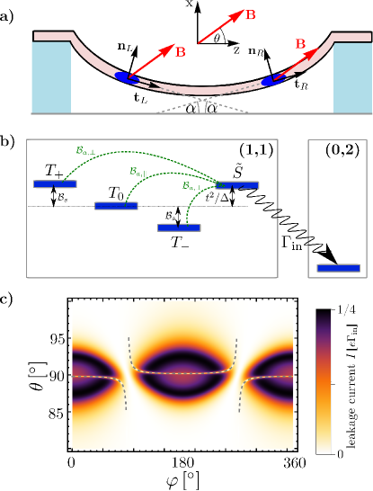
Figure 1: Pauli blockade in a bent carbon nanotube. (a) Double quantum dot in a bent CNT in a homogeneous magnetic field $B$. The direction of the magnetic field is characterized by the polar and azimuthal angles $\theta$ and $\varphi$. The geometry of the CNT is characterized by the deflection angle $\alpha$. (b) Level diagram in the inelastic interdot tunneling regime [cf. Eq. (21)]. Dashed lines represent matrix elements mixing the triplet states with the singlet $\tilde{S}$. (c) Theoretical result for the magnetic anisotropy of the leakage current $I(\varphi,\theta)$ at $B=0.5$ T, showing features similar to the measured data (Fig. S7 in the Supplementary Information of Ref. Pei et al., 2012). Dashed grey line shows the position of the antiresonance as described by the analytical formula Eq. (26). Parameter values: $\alpha=3^{\circ}$, $g_{\parallel}=32$, $E_{\tilde{S}}\equiv t^{2}/\Delta=5\,\mu$eV, $g_{\perp}^{(L)}=1.125$, $g_{\perp}^{(R)}=0.75$, $\gamma=0$. See Sec. IV for more details.

Recent advances enable the fabrication of ultraclean individual carbon nanotubes (CNTs) with exceptional electronic and mechanical qualityCao et al. (2005); Kuemmeth et al. (2008); Jespersen et al. (2011); Hüttel et al. (2009); Steele et al. (2009a, b); Wu et al. (2010); Pei et al. (2012); Laird et al. (2013); Waissman et al. (2013); Benyamini et al. (2014). Transport experimentsLaird et al. in such devices are aiming at, e.g., establishing strongly correlated electronic phasesDeshpande and Bockrath (2008); Pecker et al. (2013), controlling the CNT’s electronic and mechanical degrees of freedom and their interactionsSazonova et al. (2004); Steele et al. (2009a); Lassagne et al. (2009); Benyamini et al. (2014); Poot and van der Zant (2012), and electron-spin-based quantum information processingBulaev et al. (2008); Churchill et al. (2009); Flensberg and Marcus (2010); Pei et al. (2012); Laird et al. (2013).

Characteristic of CNTs is the coexistence of mechanical flexibility and strong spin-orbit interactionAndo (2000); Kuemmeth et al. (2008); Jeong and Lee (2009); Izumida et al. (2009). In combination with electrical confinement in CNT quantum dots (QDs), their interplay allows for strong spin-phonon couplingBulaev et al. (2008); Rudner and Rashba (2010); Pályi et al. (2012), bend-induced and electrically controlled g-tensor modulationLai et al. (2014), electrically driven spin resonanceFlensberg and Marcus (2010); Laird et al. (2013); Széchenyi and Pályi (2014); Wang and Burkard (2014); Li et al. (2014); Osika et al. (2014), spin-based motion sensingOhm et al. (2012), and mechanical readout of spin-based quantum bitsStruck et al. (2014).

In this work, we provide a theoretical description of a recently realized experimental setupPei et al. (2012), where the Pauli blockade transport effect was measured in a double QD (DQD) embedded in a bent CNT. A schematic of the setup is shown in Fig. 1a. In the Pauli blockadeOno et al. (2002); Jouravlev and Nazarov (2006); Koppens et al. (2005); Buitelaar et al. (2008), electronic transport through the serially coupled DQD proceeds via the (1,1) $\to$ (0,2) $\to$ (0,1) $\to$ (1,1) cycle of transitions, where $(N_{L},N_{R})$ denotes the numbers of electrons in the neighboring QDs.

First, consider the case when the only internal degree of freedom of the electrons is the spin, and hence the current flow is influenced by the spin selection rules of the transitions of the transport cycle. This case is relevant for, e.g., III-V semiconductorsOno et al. (2002); Fransson and Rasander (2006); Jouravlev and Nazarov (2006), and CNTs with strong disorderBuitelaar et al. (2008); Chorley et al. (2011). In the absence of singlet-triplet mixing, the (1,1) $\to$ (0,2) transition is forbidden for the triplet states by Pauli’s exclusion principle, hence the current is zero. This blockade is lifted by spin perturbations causing singlet-triplet mixing (e.g., spin-orbit interaction, hyperfine interaction, inhomogeneous magnetic field), inducing a nonzero leakage current. In turn, measurement of the leakage current can be used to characterize the spin Hamiltonian governing the current-carrying electrons. The Pauli-blockade mechanism is also utilised for qubit initialisation and readout in experimentsPetta et al. (2005); Koppens et al. (2006); Hanson et al. (2007) demonstrating coherent control of few-electron quantum bits.

In ultraclean CNT DQDs, the valley degree of freedom of the electrons and the large spin-orbit interaction play essential roles in Pauli blockade. In the limit of vanishing valley mixing, and in the absence of an external magnetic field, the ground-state doublet in each QD is a Kramers pair, usually denoted by $|K\uparrow\rangle$ and $|K^{\prime}\downarrow\rangle$, with opposite spin orientation and different valley index. The phenomenology of Pauli blockade, also called spin-valley blockadePályi and Burkard (2009, 2010) or valley-spin blockadePei et al. (2012) in this context, remains similar to the spinful case: triplet-like two-electron states composed from $|K\uparrow\rangle$ and $|K^{\prime}\downarrow\rangle$ block the current in the absence of singlet-triplet mixing, and this blockade can be lifted by spin- or valley perturbations acting differently in the two QDs.

Here, we present a model for the Pauli-blockade transport effect in a DQD embedded in a bent CNT. We take into account the strong g-factor anisotropy which is linked to the local orientation of the nanotube axis in each QD (see Fig. 1a). We provide a set of conditions under which our model can be mapped to the spin-blockade model of Jouravlev and NazarovJouravlev and Nazarov (2006). We calculate the dependence of the leakage current on the orientation of the external magnetic field. The results we obtain, see e.g., Fig. 1c, provide a possible interpretation of previously unexplained experimental resultsPei et al. (2012). Furthermore, we find that in a certain parameter range, the leakage current becomes highly sensitive to the shape of the tube, and this sensitivity increases with increasing g-factor anisotropy. This mutual dependence of the electron transport and the tube shape allows for mechanical control of the leakage current, and for characterization of the tube shape via measuring the leakage current.

II Magnetic anisotropy of the leakage current

Our aim in this work is to quantify the relation between the Pauli-blockade leakage current and the system parameters, including the shape of the CNT and the magnetic field vector. A schematic of the setup, along with the reference frame, is shown in Fig. 1(a). The magnetic field vector is characterized by its magnitude $B$ and its usual polar $\theta$ and azimuthal $\varphi$ angles, $\text{\boldmath{$B$}}=B(\sin\theta\cos\varphi,\sin\theta\sin\varphi,\cos\theta)$.

For our analysis, experimental guidance is provided by the data of Ref. Pei et al., 2012. There, an especially useful data set is presented in Fig. S7 of the Supplementary Information of Ref. Pei et al., 2012 (to be referred to as S7 from now on). In S7, the dependence of the leakage current on the magnetic field direction is plotted, in the case where the (1,1)-(0,2) energy detuning (defined below) $\Delta\sim 1$ meV and the magnetic field strength $B=0.5$ T are held fixed. Importantly, the detuning $\Delta$ was chosen such that it exceeds the Zeeman splittings for any magnetic field direction in the angular range covered in S7. Furthermore, the current shown in S7 is presumably the result of inelastic, e.g., phonon-emission-mediated, energetically downhill (1,1) $\to$ (0,2) charge transitions (as depicted by the wavy arrow in Fig. 1b), as suggested by the detuning asymmetry of the current in the corresponding data shown in Fig. 4a of Ref. Pei et al., 2012.

This measurement setting of S7 simplifies the interpretation of the data: it suggests that the rate $\Gamma_{\rm in}$ of the inelastic downhill (1,1) $\to$ (0,2) tunneling process is hardly sensitive to the magnetic field direction, hence the observed field-direction dependence of the leakage current is caused by the field-direction-induced variations of the four energy eigenstates of the (1,1) charge configuration, and not by variations of the tunnel rate $\Gamma_{\rm in}$.

The main features seen in S7 are as follows. (E1) In a narrow range of $\theta\in[85^{\circ},95^{\circ}]$, i.e., for magnetic field directions almost perpendicular to the CNT axis, the leakage current is much higher ($\sim 10$ pA) than outside that range ($\lesssim 1$ pA). (E2) Apparently, the high-current region is defined by the condition $|\theta-\pi/2|<A\cos\varphi$, where $A\approx 5^{\circ}$. (E3) The high-current regions are separated by low-current gaps at $\varphi\approx 90^{\circ}$ and $\varphi\approx 270^{\circ}$. Two weaker features of S7: (E4) There are two narrow lines of reduced current (antiresonances) around $\theta\approx 90^{\circ}$, approximately horizontal at $\varphi\approx 0$ ($\varphi\approx 180^{\circ}$) but bending downward (upward) as $\varphi$ is moved away from $0$ ($180^{\circ}$). (E5) There are two narrow lines of increased current (resonances), at $(\varphi,\theta)\approx(0^{\circ},98^{\circ})$ [$(\varphi,\theta)\approx(180^{\circ},82^{\circ})$], bending downward [upward] as $\varphi$ is moved away from $0$ [$180^{\circ}$].

Among the theoretical works addressing few-electron physics in CNT DQDsPályi and Burkard (2009); Weiss et al. (2010); Pályi and Burkard (2010); von Stecher et al. (2010); Reynoso and Flensberg (2011, 2012); Kiss et al. (2011); Széchenyi and Pályi (2013); Li et al. (2014), Refs. Pályi and Burkard, 2010; Széchenyi and Pályi, 2013 described the Pauli blockade transport effect in the case of a straight CNT. In Ref. Széchenyi and Pályi, 2013, we found that the Pauli blockade can be lifted if the external magnetic field is perpendicular to the CNT axis. That finding is in line with the experimental feature (E1) seen in the bent CNT. However, for the straight CNT, the current is independent of the azimuth angle $\varphi$ of the field, because of the cylindrical symmetry of the straight geometry. This is in contrast with the experimental features (E2)-(E5), which motivates the present study accounting for the bent shape of the CNT. The model we present will provide possible explanations of the features (E1)-(E4) observed in S7, as demonstrated by Fig. 1c.

III Model

The setup, consisting of an electrostatically defined DQD in a bent CNT, is shown in Fig 1a. In our model, the shape of the CNT is characterized by the unit vectors $\text{\boldmath{$t$}}_{D}$ ($D=L,R$) along the local CNT axes in the two QDs $L$ and $R$. The reference frame (see Fig. 1a) is chosen such that these unit vectors span the $x$-$z$ plane and are characterized by a single angle parameter $\alpha$, which we refer to as the deflection angle:

$$\text{\boldmath{$t$}}_{L} = (-\sin\alpha,0,\cos\alpha),$$ (1a)

$$\text{\boldmath{$t$}}_{R} = (\sin\alpha,0,\cos\alpha).$$ (1b)

The deflection angle is assumed to be smallLaird et al. (2013), $\alpha\ll 1$. We also introduce the unit vectors $\text{\boldmath{$n$}}_{L}=(\cos\alpha,0,\sin\alpha)$, $\text{\boldmath{$n$}}_{R}=(\cos\alpha,0,-\sin\alpha)$, and $\text{\boldmath{$n$}}^{\prime}_{D}=\text{\boldmath{$t$}}_{D}\times\text{\boldmath{$n$}}_{D}$, see Fig. 1a.

III.1 Single-electron Hamiltonian

The $4\times 4$ Hamiltonian describing a single electron occupying the nominally fourfold (spin and valley) degenerate ground-state orbital of QD $D$ readsFlensberg and Marcus (2010); Rudner and Rashba (2010)

$$H_{D} = -\frac{\Delta_{\textrm{SO}}^{(D)}}{2}\text{\boldmath{$t$}}_{D}\cdot\text{\boldmath{$s$}}\,\tau_{3}+\frac{\Delta_{KK^{\prime}}^{(D)}}{2}\left(\cos{\gamma^{(D)}}\tau_{1}+\sin{\gamma^{(D)}}\tau_{2}\right)$$ (2)

$$+ H_{B,D},$$

where

$$H_{B,D} = \frac{1}{2}g_{s}\mu_{B}\text{\boldmath{$B$}}\mbox{\boldmath{$s$}}+\frac{1}{2}g_{v}^{(D)}\mu_{B}\text{\boldmath{$t$}}_{D}\cdot\text{\boldmath{$B$}}\,\tau_{3}.$$ (3)

Furthermore, $\text{\boldmath{$s$}}=(s_{x},s_{y},s_{z})$ and $\boldsymbol{\tau}=(\tau_{1},\tau_{2},\tau_{3})$ are the vectors of Pauli matrices in the spin and valley spaces, respectively, $\Delta_{\textrm{SO}}^{(D)}$ is the spin-orbit splitting in QD $D$, $\Delta_{KK^{\prime}}^{(D)}e^{i\gamma^{(D)}}$ is the complex valley-mixing matrix element in QD $D$, and the last two terms describe the Zeeman splittings, where $g_{s}$ ($g_{v}^{(D)}$) is the spin (orbital) g-factor (in QD $D$). We assume $\Delta_{\rm SO}^{(D)}>0$ and $g_{v}^{(D)}>0$. In Eq. (2), the unit matrices in spin ($s_{0}$) and valley ($\tau_{0}$) space are suppressed.

The $8\times 8$ single-electron Hamiltonian of the DQD incorporates spin- and valley-conserving interdot tunnelling:

$$H_{\rm DQD}=H_{L}\eta_{L}+H_{R}\eta_{R}+H_{\rm tun},$$ (4)

where $\eta_{L/R}=(\eta_{0}\pm\eta_{3})/2$,

$$H_{\rm tun}=\frac{t}{\sqrt{2}}s_{0}\tau_{0}\eta_{1},$$ (5)

and $\eta_{0,1,2,3}$ are the Pauli matrices acting on the spatial degree of freedom $(L,R)$. Furthermore, $t$ is real-valued.

At zero magnetic field $\text{\boldmath{$B$}}=0$ and zero interdot tunnelling $t=0$, the energy eigenstates of $H_{\rm DQD}$ form four Kramers doublets at energies $\pm\sqrt{[\Delta^{(D)}_{\rm SO}]^{2}+[\Delta^{(D)}_{KK^{\prime}}]^{2}}$. Here we focus on the low-energy doublets in both dots, to be denoted by

$$|\tilde{\Uparrow}_{D}\rangle = \cos{\frac{\chi^{(D)}}{2}}|K\uparrow_{D}\rangle-\sin{\frac{\chi^{(D)}}{2}}e^{i\gamma^{(D)}}|K^{\prime}\uparrow_{D}\rangle,$$ (6a)

$$|\tilde{\Downarrow}_{D}\rangle = \cos{\frac{\chi^{(D)}}{2}}|K^{\prime}\downarrow_{D}\rangle-\sin{\frac{\chi^{(D)}}{2}}e^{-i\gamma^{(D)}}|K\downarrow_{D}\rangle,$$ (6b)

where $K$ and $K^{\prime}$ are the valley basis states, $\uparrow_{D}$ ($\downarrow_{D}$) is the spin-up (spin-down) state in QD $D$ with spin quantization axis $\text{\boldmath{$t$}}_{D}$, and $\chi^{(D)}=\arctan\left(\Delta_{KK^{\prime}}^{(D)}/\Delta_{\rm SO}^{(D)}\right)\in[0,\pi/2[$.

In order to provide an approximate mapping of our model of the CNT DQD to the model of Ref. Jouravlev and Nazarov, 2006 (see next subsection), we introduce the following gauge-transformed states:

$$|\Uparrow_{L}\rangle = e^{i\xi/2}|\tilde{\Uparrow}_{L}\rangle,$$ (7a)

$$|\Downarrow_{L}\rangle = e^{-i\xi/2}|\tilde{\Downarrow}_{L}\rangle,$$ (7b)

$$|\Uparrow_{R}\rangle = e^{-i\xi/2}|\tilde{\Uparrow}_{R}\rangle,$$ (7c)

$$|\Downarrow_{R}\rangle = e^{i\xi/2}|\tilde{\Downarrow}_{R}\rangle,$$ (7d)

where

$$\xi=\arctan\left(\frac{\sin\gamma^{\prime}\sin\frac{\chi^{(L)}}{2}\sin\frac{\chi^{(R)}}{2}}{\cos\frac{\chi^{(L)}}{2}\cos\frac{\chi^{(R)}}{2}+\cos\gamma^{\prime}\sin\frac{\chi^{(L)}}{2}\sin\frac{\chi^{(R)}}{2}}\right),$$ (8)

and $\gamma^{\prime}=\gamma^{(R)}-\gamma^{(L)}$. The states defined in Eqs. (7a) and (7b) [Eqs. (7c) and (7d)] will be referred to as the Kramers-qubit basis states in QD $L$ [$R$].

III.2 Low-energy single-electron Hamiltonian

We assume conditions when only the four lowest-energy single-particle energy levels of the DQD, i.e., $|\!\!\!\Uparrow_{L}\rangle$, $|\!\!\!\Downarrow_{L}\rangle$, $|\!\!\!\Uparrow_{R}\rangle$, and $|\!\!\!\Downarrow_{R}\rangle$, participate in the (1,1)$\to$(0,2)$\to$(0,1)$\to$(1,1) Pauli-blockade transport cycle. The effects of interdot tunnelling and the external magnetic field are treated in first-order perturbation theory. That is, we project the $8\times 8$ single-electron Hamiltonian $H_{\rm DQD}$ to the $4\times 4$ subspace spanned by the four states above, i.e,

$$H^{\prime}_{\rm DQD}\equiv PH_{\rm DQD}P,$$ (9)

where

$$P=\sum_{D=L,R}\left(|\Uparrow_{D}\rangle\langle\Uparrow_{D}|+|\Downarrow_{D}\rangle\langle\Downarrow_{D}|\right).$$ (10)

The low-energy Hamiltonian $H^{\prime}_{\rm DQD}$ provides a good approximation for the dynamics as long as the spin and orbital Zeeman splittings and the interdot tunnelling $t$ are all much smaller than the energy splittings $2\sqrt{[\Delta^{(D)}_{\rm SO}]^{2}+[\Delta^{(D)}_{KK^{\prime}}]^{2}}$ induced by spin-orbit interaction and valley mixing.

Omitting a constant diagonal term in $H^{\prime}_{\rm DQD}$, it can be written as $H^{\prime}_{\rm DQD}=H^{\prime}_{B}+H^{\prime}_{\rm tun}$. As shown below, the homogeneous magnetic field is felt by the Kramers-qubit in QD $D$ as a local effective magnetic fieldFlensberg and Marcus (2010); Széchenyi and Pályi (2013) $\text{\boldmath{$\mathcal{B}$}}_{D}$. This is made explicit by casting the low-energy magnetic Hamiltonian for the DQD in the following form:

$$H^{\prime}_{B}\equiv PH_{B}P=\frac{1}{2}\left[\text{\boldmath{$\mathcal{B}$}}_{L}\text{\boldmath{$\sigma$}}_{L}+\text{\boldmath{$\mathcal{B}$}}_{R}\text{\boldmath{$\sigma$}}_{R}\right].$$ (11)

Here, $\text{\boldmath{$\sigma$}}_{D}$ is the vector of Pauli matrices corresponding to the Kramers-qubit basis states in QD $D$, e.g., $\sigma_{L,3}=|\Uparrow_{L}\rangle\langle\Uparrow_{L}|-|\Downarrow_{L}\rangle\langle\Downarrow_{L}|$. The effective magnetic field $\text{\boldmath{$\mathcal{B}$}}_{D}$ is related to the external magnetic field $B$ via

$$\mathcal{B}_{D1} = -g_{\perp}^{(D)}\mu_{B}\textrm{Re}\left[(B_{Dn}+iB_{Dn^{\prime}})e^{i(\gamma^{(D)}+D\xi)}\right],$$ (12a)

$$\mathcal{B}_{D2} = -g_{\perp}^{(D)}\mu_{B}\textrm{Im}\left[(B_{Dn}+iB_{Dn^{\prime}})e^{i(\gamma^{(D)}+D\xi)}\right],$$ (12b)

$$\mathcal{B}_{D3} = g_{\parallel}^{(D)}\mu_{B}B_{Dt},$$ (12c)

where $D\in(L,R)\equiv(+1,-1)$, and

$$g_{\perp}^{(D)} = g_{s}\sin{\chi^{(D)}},$$ (13a)

$$g_{\parallel}^{(D)} = g_{s}+g_{v}^{(D)}\cos{\chi^{(D)}},$$ (13b)

and we introduced the projections of the the external magnetic field on the local coordinate axes via

$$B_{Dt} = \text{\boldmath{$t$}}_{D}\cdot\text{\boldmath{$B$}},$$ (14a)

$$B_{Dn} = \text{\boldmath{$n$}}_{D}\cdot\text{\boldmath{$B$}},$$ (14b)

$$B_{Dn^{\prime}} = \text{\boldmath{$n$}}^{\prime}_{D}\cdot\text{\boldmath{$B$}}.$$ (14c)

Henceforth, we will refer to $\mathcal{B}_{D1}$ and $\mathcal{B}_{D2}$ ($\mathcal{B}_{D3}$) as the transverse components (longitudinal component) of the effective field, and $g_{\perp}^{(D)}$ ($g_{\parallel}^{(D)}$) as the transverse (longitudinal) g factor.

We further define the symmetric $\text{\boldmath{$\mathcal{B}$}}_{s}=\frac{1}{2}\left(\text{\boldmath{$\mathcal{B}$}}_{L}+\text{\boldmath{$\mathcal{B}$}}_{R}\right)$ and the antisymmetric $\text{\boldmath{$\mathcal{B}$}}_{a}=\frac{1}{2}\left(\text{\boldmath{$\mathcal{B}$}}_{L}-\text{\boldmath{$\mathcal{B}$}}_{R}\right)$ combinations of the effective magnetic fields, and the component $\text{\boldmath{$\mathcal{B}$}}_{a,\parallel}$ ($\text{\boldmath{$\mathcal{B}$}}_{a,\perp}$) of the antisymmetric combination that is parallel (perpendicular) to $\text{\boldmath{$\mathcal{B}$}}_{s}$.

The single-electron tunnelling Hamiltonian in the low-energy subspace reads $H^{\prime}_{\rm tun}\equiv PH_{\rm tun}P$. We focus on cases where our model, at least approximately, can be mapped to that of Ref. Jouravlev and Nazarov, 2006. To see when that can be done, let us recall a key feature of the model of Ref. Jouravlev and Nazarov, 2006: there is no tunneling between the (1,1) triplet states and the (0,2) singlet state. This is ensured by the fact that tunnelling is assumed to be spin-conserving, i.e., in any spin basis, the single-electron tunnelling matrix elements are the same for the up-spin and down-spin electrons. In order to have the analogous feature, at least approximately, in our model, our tunneling Hamiltonian $H^{\prime}_{\rm tun}$ should satisfy the following two conditions. (i) Qubit-flip tunnelling should be much weaker than qubit-conserving tunnelling, i.e., $|\langle\Uparrow_{L}|H_{\rm tun}|\Downarrow_{R}\rangle|,|\langle\Uparrow_{R}|H_{\rm tun}|\Downarrow_{L}\rangle|\ll|\langle\Uparrow_{L}|H_{\rm tun}|\Uparrow_{R}\rangle|,|\langle\Downarrow_{L}|H_{\rm tun}|\Downarrow_{R}\rangle|$. (ii) The qubit-conserving tunnel amplitudes should be equal, $\langle\Uparrow_{L}|H_{\rm tun}|\Uparrow_{R}\rangle=\langle\Downarrow_{L}|H_{\rm tun}|\Downarrow_{R}\rangle$. Condition (i) is ensured if $\Delta^{(D)}_{\rm SO}\geq\Delta_{KK^{\prime}}^{(D)}$ and $\alpha\ll 1$, which we assume from now on. By explicit evaluation of the matrix elements of $H_{\rm tun}$, we find that the relation $\Delta^{(D)}_{\rm SO}\geq\Delta_{KK^{\prime}}^{(D)}$ guarantees that the ratio of the qubit-flip and qubit-conserving matrix elements fulfills

$$\frac{|\langle\Uparrow_{L}|H_{\rm tun}|\Downarrow_{R}\rangle|}{|\langle\Uparrow_{L}|H_{\rm tun}|\Uparrow_{R}\rangle|}\leq\sqrt{2}\tan\alpha\ll 1,$$ (15)

hence the qubit-flip matrix elements can indeed be neglected to a good approximation. Condition (ii) is ensured by the gauge choice specified by Eqs. (7) and (8). (See also the discussion in Appendix C of Ref. Li et al., 2014.) In fact, this gauge also guarantees that the qubit-conserving tunnel amplitudes $\langle\Uparrow_{L}|H_{\rm tun}|\Uparrow_{R}\rangle$ and $\langle\Downarrow_{L}|H_{\rm tun}|\Downarrow_{R}\rangle$ are real-valued, but that is not essential.

III.3 Two-electron Hamiltonian

We consider the Pauli blockade occurring in the DQD in the transport cycle $(0,1)\rightarrow(1,1)\rightarrow(0,2)\rightarrow(0,1)$. We denote the energy detuning between the (1,1) and (0,2) charge configurations by $\Delta$. Together with the preceding assumptions, this provides the $5\times 5$ two-electron Hamiltonian

$$H^{\prime}=H^{\prime}_{B}+t\left(|S\rangle\langle S_{g}|+|S_{g}\rangle\langle S|\right)-\Delta|S_{g}\rangle\langle S_{g}|$$ (16)

Here $H^{\prime}_{B}$ is the two-electron generalisation of the single-electron Hamiltonian in Eq. (11). Furthermore, $|S\rangle$ [$|S_{g}\rangle$] denotes the singlet state in the (1,1) [(0,2)] charge configuration, formed from the local Kramers-qubit basis states. Note that through the preceding steps, we mapped the Pauli blockade problem in the bent CNT to the model of Jouravlev and Nazarov Jouravlev and Nazarov (2006), originally developed to describe spin blockade in GaAs in the presence of nuclear spins.

As discussed in Sec. II, the current shown in S7 is presumably the result of inelastic (1,1) $\to$ (0,2) charge transitions. Therefore we focus on the large-detuning case $\Delta\gg t$, and introduce the inelastic tunneling rate $\Gamma_{\rm in}$ characterizing qubit-state-conserving incoherent transitions from the (1,1) to the (0,2) charge configuration. We eliminate the coherent tunnel coupling $t$ from the Hamiltonian via perturbation theory, resulting in ‘dressed’ singlet states $|\tilde{S}\rangle$ and $|\tilde{S}_{g}\rangle$. The resulting $4\times 4$ Hamiltonian describing the (1,1) charge configuration reads

$$H^{\prime\prime}=\left(\begin{array}[]{cccc}\mathcal{B}_{s}&0&0&-\mathcal{B}_{a,\perp}/\sqrt{2}\\ 0&0&0&\mathcal{B}_{a,\parallel}\\ 0&0&-\mathcal{B}_{s}&\mathcal{B}_{a,\perp}/\sqrt{2}\\ -\mathcal{B}_{a,\perp}/\sqrt{2}&\mathcal{B}_{a,\parallel}&\mathcal{B}_{a,\perp}/\sqrt{2}&E_{\tilde{S}}\\ \end{array}\right).$$ (21)

The basis we use here is $T_{+},T_{0},T_{-},\tilde{S}$, where the triplet states are defined as usual, but in a rotated qubit reference frameJouravlev and Nazarov (2006) where the third axis is aligned with $\text{\boldmath{$\mathcal{B}$}}_{s}$ and the first axis is aligned with $\text{\boldmath{$\mathcal{B}$}}_{a,\perp}$. Furthermore, $E_{\tilde{S}}=t^{2}/\Delta$.

The structure of the Hamiltonian $H^{\prime\prime}$ is visualised in Fig. 1b. The symmetric combination of the effective magnetic fields $\text{\boldmath{$\mathcal{B}$}}_{s}$ splits the three triplet states, whereas the antisymmetric combination $\text{\boldmath{$\mathcal{B}$}}_{a}$ is responsible for mixing the triplet states with the dressed (1,1) singlet $\tilde{S}$. The Hamiltonian $H^{\prime\prime}$ allows us to identify special cases where the current is zeroJouravlev and Nazarov (2006); Danon et al. (2013). If $\mathcal{B}_{a,\perp}=0$ ($\mathcal{B}_{a,\parallel}=0$), then $T_{+}$ and $T_{-}$ ($T_{0}$) decouple from $\tilde{S}$, and hence block the current. Another special case with zero current is $B_{s}=0$: in this case, a certain superposition of the three triplets forms a dark state which is decoupled from $\tilde{S}$, and this dark state will block the current.

III.4 Rate equation for the leakage current

The leakage current is calculated as follows. First, we diagonalize $H^{\prime\prime}$ to obtain its eigenstates $|i\rangle$ $(i=1,2,3,4)$. Then, since qubit-flip tunnelling is negligible, the (1,1) $\to$ (0,2) transition rate $\Gamma_{i}$ for each eigenstate $|i\rangle$ is assumed to be proportional to its $|\tilde{S}\rangle$ weight: $\Gamma_{i}=\Gamma_{\rm in}\left|\langle\tilde{S}|i\rangle\right|^{2}$. After reaching the (0,2) singlet state, one electron from QD $R$ exits to the drain, and one enters to QD $L$ from the source. These steps are characterized by the filling rate $\Gamma_{\rm f}$ and a corresponding probability $p_{0}$ of being either in the (0,2) or in the (0,1) charge configuration. These considerations result in the following rate equations:

$$\dot{p}_{i} = -\Gamma_{i}p_{i}+\frac{1}{4}\Gamma_{\rm f}p_{0}\ \ \ \ \ \ (i=1,2,3,4)$$ (22a)

$$\dot{p}_{0} = -\Gamma_{\rm f}p_{0}+\sum_{i=1}^{4}\Gamma_{i}p_{i}.$$ (22b)

where $p_{i}$ ($i=1,2,3,4$) is the occupation probability of the (1,1) eigenstate $|i\rangle$. Normalization condition $p_{0}+\sum_{i=1}^{4}p_{i}=1$ also applies.

We focus on the case when the bottleneck is the inelastic interdot tunneling, i.e., $\Gamma_{\rm in}\ll\Gamma_{\rm f}$. Then, the steady-state probabilities are $p_{0}\approx 0$ and $p_{i}\approx\frac{1}{\Gamma_{i}\mathcal{T}}$ with $\mathcal{T}=\sum_{i=1}^{4}\Gamma_{i}^{-1}$. The steady-state leakage current is obtained via $I=e\sum_{i=1}^{4}p_{i}\Gamma_{i}=4e/\mathcal{T}$.

IV Results

In this section, we provide and discuss the results for the magnetic anisotropy of the leakage current, and provide the corresponding geometrical interpretations based on the effective magnetic field vectors $\text{\boldmath{$\mathcal{B}$}}_{D}$.

The effective magnetic fields $\text{\boldmath{$\mathcal{B}$}}_{D}$ given in Eq. (12) apparently depend explicitly on the complex phases $\gamma^{(D)}$ of the valley-mixing matrix elements as well as the phase $\xi$ used for fixing the gauge. However, it can be shown that the only combination of these parameters that influences the current through the DQD is $\gamma\equiv\gamma^{(R)}-\gamma^{(L)}-2\xi$. Therefore, for our forthcoming results we specify the value of the parameter $\gamma$. Similarly, instead of specifying the values of the parameters $\Delta_{KK^{\prime}}^{(D)}$, $\Delta_{\rm SO}^{(D)}$, $g_{v}^{(D)}$ of our original model, we specify the values of the derived parameters $g_{\perp}^{(D)}$, $g_{\parallel}^{(D)}$, and $E_{\tilde{S}}$. For simplicity, we choose identical longitudinal g-factors in the two QDs, $g_{\parallel}\equiv g_{\parallel}^{(L)}=g_{\parallel}^{(R)}$.

IV.1 Analytical results for the $E_{\tilde{S}}$ = 0 case

In the special case $E_{\tilde{S}}=0$, the following analytical result is obtainedJouravlev and Nazarov (2006) for the leakage current:

$$I=\frac{1}{4}e\Gamma_{\rm in}(\text{\boldmath{$\hat{\mathcal{B}}$}}_{L}\times\text{\boldmath{$\hat{\mathcal{B}}$}}_{R})^{2},$$ (23)

where $\text{\boldmath{$\hat{\mathcal{B}}$}}_{D}=\text{\boldmath{$\mathcal{B}$}}_{D}/\mathcal{B}_{D}$. This result implies that the maximal current is $e\Gamma_{\rm in}/4$, and the current has this maximal value if $\text{\boldmath{$\mathcal{B}$}}_{L}\perp\text{\boldmath{$\mathcal{B}$}}_{R}$, i.e., $\text{\boldmath{$\mathcal{B}$}}_{L}\cdot\text{\boldmath{$\mathcal{B}$}}_{R}=0$.

The magnetic anisotropy of the leakage current (23) for a certain parameter set is shown in Fig. 2a-f. Focus on Figs. 2a,d,g first, which corresponds to relatively small transverse g-factor values.

To understand the results shown in Figs. 2a,d,g it is instructive to consider the case of infinitesimally small transverse g factors (i.e., infinitesimally weak valley mixing). In that limit, after expanding the maximal-current condition $\text{\boldmath{$\mathcal{B}$}}_{L}\cdot\text{\boldmath{$\mathcal{B}$}}_{R}=0$ up to second order in $\theta-\pi/2\ll 1$ and $\alpha\ll 1$, we obtain

$$\theta=\pi/2\pm\alpha\cos\varphi,$$ (24)

i.e., the maximal current $e\Gamma_{\rm in}/4$ is flowing for magnetic field directions $(\varphi,\theta)$ fulfilling Eq. (24). This makes sense: e.g., for $\varphi=0$ and $\theta=\pi/2+\alpha$, the external magnetic field is aligned with $\text{\boldmath{$n$}}_{L}$, hence the effective field $\text{\boldmath{$\mathcal{B}$}}_{L}$ is purely transversal, whereas $\text{\boldmath{$\mathcal{B}$}}_{R}$ is dominated by its longitudinal component, i.e., these two vectors are indeed perpendicular.

Moreover, in the limit of infinitesimal transverse g factors, current is finite only in the infinitesimal vicinity of the two maximal-current curves described by Eq. (24). Otherwise the current is suppressed, for the following reason. If $\theta\neq\pi/2\pm\alpha\cos\varphi$, then the longitudinal effective fields are finite in both dots and they dominate over the infinitesimally small transverse effective fields. Then the effective field vectors are almost parallel, hence, according to Eq. (23), the current is almost zero. This is exemplified in Figs. 2a,d,g, where the transverse g factors are set to relatively small values, and hence the leakage current is significant only in the close vicinity of the lines given by Eq. (24).

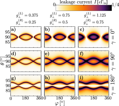
Figure 2: Magnetic anisotropy of the leakage current: dependence on transverse g factors and the phase $\gamma$. The transverse g factors $g_{\perp}^{(L,R)}$ are shown at the top of each vertical block. The phase $\gamma$ is shown at the right end of each horizontal block. Further parameters: $B=0.5$ T, $\alpha=3^{\circ}$, $g_{\parallel}=32$, $E_{\tilde{S}}=0$.

If the transverse g factors are gradually increased, as shown in Figs 2a,b,c, then the narrow maximal-current lines become broader, eventually leading to an $I(\varphi,\theta)$ pattern that is very similar to feature (E2) of S7. [Note the remarkable similarity between Fig. 2c and S7.] Another way to phrase this is that in the $(\varphi,\theta)$ points in the vicinity of the lines $\theta=\pi/2\pm\alpha\cos\varphi$, the leakage current increases with increasing transverse g factors. This effect is due to the fact that the increasing transverse g factors increase the transverse components of the effective fields $\text{\boldmath{$\mathcal{B}$}}_{D}$ (cf. Eq. (12)), driving these fields away from their infinitesimal-transverse-g-factor limit where $\text{\boldmath{$\mathcal{B}$}}_{L}\parallel\text{\boldmath{$\mathcal{B}$}}_{R}$ and the current is zero.

Another feature seen in Figs. 2a-c is a low-current gap around $\varphi=90^{\circ}$ and $\varphi=270^{\circ}$ between the high-current regions. This gap is getting larger as valley mixing is increased from Figs. 2a to Figs. 2c. This gap is absent in Figs. 2d-f, where the phase $\gamma$ is set to $\gamma=90^{\circ}$. Also, the gap is not seen in Figs. 2g-i, where $\gamma=180^{\circ}$. There, the $I(90^{\circ},\theta)$ and $I(270^{\circ},\theta)$ cuts show high-current peaks for $\theta\approx 90^{\circ}\pm 1^{\circ}$.

These effects have straightforward geometrical interpretations based on Eq. (23). Furthermore, a quantitative description of these is obtained if the maximal-current condition $\text{\boldmath{$\mathcal{B}$}}_{L}\cdot\text{\boldmath{$\mathcal{B}$}}_{R}=0$ is expanded up to second order in $\theta-\pi/2\ll 1$, $\alpha\ll 1$ and $\frac{g_{\perp}^{(D)}}{g_{\parallel}}\ll 1$, yielding the maximal-current condition

$$\theta=\frac{\pi}{2}\pm\sqrt{(\alpha\cos{\varphi})^{2}-\frac{g_{\perp}^{(L)}g_{\perp}^{(R)}}{g_{\parallel}^{2}}\cos{\gamma}}.$$ (25)

Note that this refined version (25) of Eq. (24) depends on the phase $\gamma$. The second term under the square root in Eq. (25), proportional to $\cos\gamma$, accounts for the above described $\gamma$-dependent qualitative changes in Fig. 2.

The above observations, together with the experimental data in S7, can be utilized to gain information on the experimental setup of Ref. Pei et al., 2012. In S7, the lines of maximal current are given approximately by $\theta\approx 3^{\circ}\cos\varphi$, implying that the deflection angle is approximately $3^{\circ}$. Furthermore, feature (E3) implies that $0\leq|\gamma|<\pi/2$; we use $\gamma=0$ in the rest of this paper. Finally, the fact that the leakage current at the center $(\varphi,\theta)=(0,\pi/2)$ of the high-current region is almost as high as the maximal current [at $(\varphi,\theta)\approx(0,3^{\circ})$] implies that the longitudinal and transverse effective field components at $(\varphi,\theta)=(0,\pi/2)$ are similar in magnitude, i.e. $g^{(D)}_{\perp}\sim g_{\parallel}\alpha$.

In conclusion, the analytical results for the $E_{\tilde{S}}=0$ case can describe the strong experimental features (E1), (E2) and (E3) if the model parameters are appropriately adjusted. In particular, the parameter set used in Fig. 2c results in an $I(\varphi,\theta)$ pattern that is remarkably similar to the experimental result S7. The weaker features (E4) and (E5) are not reproduced, motivating further study of the case $E_{\tilde{S}}>0$.

IV.2 Results for the $E_{\tilde{S}}>0$ case

In this case, we diagonalize the Hamiltonian $H^{\prime\prime}$ numerically to obtain the eigenstates $|i\rangle$. The magnetic anisotropy of the leakage current for specific choices of parameters close to the experimental values is shown in Fig. 3. The narrow antiresonance (E4) appears on this plot, but the resonance (E5) does not. (Note that Figs. 1c and 3a correspond to the same parameter set.)

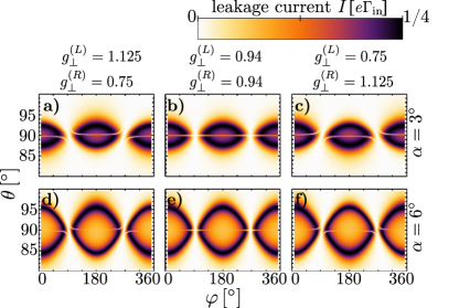
Figure 3: Magnetic anisotropy of the leakage current: antiresonance and shape-sensitivity. The transverse g factors $g_{\perp}^{(L,R)}$ are shown at the top of each vertical block. The deflection angle $\alpha$ characterizing the tube shape is shown at the right end of each horizontal block. Further parameters: $B=0.5$ T, $\gamma=0$, $g_{\parallel}=32$, $E_{\tilde{S}}=5\ \mu$eV.

The explanation of the antiresonance is as follows. For certain magnetic field directions, the effective fields in the two dots have the same magnitude $\mathcal{B}_{L}=\mathcal{B}_{R}$. In that case, $\mathcal{B}_{a,\parallel}=0$, hence the state $T_{0}$ decouples from the other three basis states in the $4\times 4$ Hamiltonian $H^{\prime\prime}$. As $T_{0}$ is decoupled from $\tilde{S}$, it cannot decay to the (0,2) singlet $\tilde{S}_{g}$, hence blocks the current flow and therefore the leakage current vanishes in this case.

The shape of the antiresonance curve on the $\theta,\varphi$ plane is described by the condition $\mathcal{B}_{L}=\mathcal{B}_{R}$, which, after linearizing in $\alpha\ll 1$ and $\theta-\pi/2\ll 1$, yields

$$\theta=\frac{\pi}{2}-\frac{\left(g_{\perp}^{(L)}\right)^{2}-\left(g_{\perp}^{(R)}\right)^{2}}{4g_{\parallel}^{2}}\frac{1}{\alpha\cos{\varphi}}.$$ (26)

Note that this result is consistent with the assumption $\theta-\pi/2\ll 1$ only if the second term of the rhs of Eq. (26) is much smaller than 1. The analytical result Eq. (26) is superimposed as a dashed line on Fig. 1c on the numerically obtained leakage-current density plot. The analytical result follows closely the narrow low-current region of the density plot. We remark that the function (26) describing the antiresonance curve is independent of the phase $\gamma$, which is a consequence of the condition $\mathcal{B}_{L}=\mathcal{B}_{R}$ being insensitive to the directions of the effective field vectors.

Recall that the antiresonance appears in Fig. (3) because $E_{\tilde{S}}\equiv t^{2}/\Delta$ is set to a nonzero value. This implies that the visibility of the antiresonance depends on $t$ and $\Delta$, and perhaps also on further system parameters. To characterize this visibility, we analytically calculate the leakage current in the vicinity of a given point $(\varphi_{0},\theta_{0})$ on the antiresonance curve. We do this by taking into account the perturbative coupling of the state $T_{0}$ to the state $\tilde{S}$ by the small matrix element $\mathcal{B}_{a,\perp}$, see Eq. (21). The leakage current is governed by the corresponding slow decay rate, and is evaluated using first-order perturbation theory in $\mathcal{B}_{a,\perp}/E_{\tilde{S}}$. This yields the following result:

$$I(\varphi_{0},\theta_{0}+\delta\theta)=c\left(\frac{\Delta\mu_{B}B}{t^{2}}\right)^{2}\alpha^{2}\cos^{2}{\varphi_{0}}\,\delta\theta^{2}e\Gamma_{\rm{in}},$$ (27)

where

$$c=16\frac{g_{\parallel}^{4}}{|g_{\perp}^{(L)}+g_{\perp}^{(R)}e^{i\gamma}|^{2}}.$$ (28)

Importantly, the prefactor of $\delta\theta^{2}$ in Eq. (27) decreases as $t^{2}/\Delta$ increases. Therefore, increasing $t^{2}/\Delta$ increases the width of the antiresonance along the $\theta$ direction, hence increases the visibility of the antiresonance. This is in line with our observations, i.e., with the appearance of the antiresonance upon increasing $t^{2}/\Delta$ from zero [Fig. 2c] to a finite value [Fig. 3a].

We note that an antiresonance effect similar to that in Fig. 3 has been discussed in Ref. Jouravlev and Nazarov, 2006 for GaAs DQDs with isotropic g-tensors and isotropic hyperfine interaction. However, to our knowledge, such an antiresonance (called ‘stopping point’ in Ref. Jouravlev and Nazarov, 2006) has not been observed in GaAs DQDs. The reason is probably that the external magnetic field vector corresponding to a stopping point in GaAs depends on the nuclear spin configuration, and the latter typically changes significantly during a current measurement; hence the stopping points are averaged out and the measured current appears to be a smooth function of the magnetic field. Another type of stopping point, corresponding to the condition $\text{\boldmath{$\mathcal{B}$}}_{s}=0$, has been discussed in Ref. Danon et al., 2013.

Figures 3a-f also demonstrate, in line with Eq. (26), that the $L$/$R$ asymmetry in the transverse g factors is directly observable as the orientation of the antiresonance curve on the $I(\varphi,\theta)$ plot. E.g., the antiresonance curve in the $90^{\circ}<\varphi<270^{\circ}$ interval bends upwards (downwards) if the transverse g factor is greater in QD $L$ ($R$), and it is a flat line if the transverse g factors are equal.

IV.3 Shape sensitivity of the leakage current

We use Fig. 3 to demonstrate the dependence of the leakage current on the DQD’s deflection angle $\alpha$. The first line (Fig. 3a-c) shows the magnetic anisotropy of the leakage current for $\alpha=3^{\circ}$, whereas the second line (Fig. 3d-f) shows that for $\alpha=6^{\circ}$. As predicted by Eq. (24), the region of maximal current is focused around the lines $\theta=\pi/2\pm\alpha\cos\varphi$. It is clear from Eq. (26), although less obvious from Fig. 3, that the antiresonance line moves as the angle $\alpha$ is changed.

In Fig. 4, we show how the leakage current depends on the deflection angle $\alpha$ characterizing the shape of the CNT for a fixed magnetic field. To this end, we pick the points $(\varphi,\theta)=(180^{\circ},96^{\circ})$ in Figs. 3a d, and plot the leakage current for this magnetic field orientation as the deflection angle is varied continuously. This is shown as the green dashed line in Fig. 4, which displays a broad peak around $\alpha=6^{\circ}$. The other two lines correspond to smaller transverse g factors (i.e., smaller valley-mixing matrix elements or larger spin-orbit splittings), resulting in narrowed current peaks.

The results shown in Fig. 4 suggest that the in situ changes in the shape of the CNT could in principle be monitored by measuring the current flowing through the embedded DQD. Static variations in $\alpha$ with respect to a reference value (‘working point’) $\alpha_{0}$ could be effectively detected if the slope of the $I(\alpha)$ curve is large at the reference value $\alpha_{0}$. For example, if the system is described by the solid red curve of Fig. 4, then, e.g., $\alpha_{0}\approx 5.5^{\circ}$ is a good working point. Dynamical variation of $\alpha$, due to, e.g., external driving of a flexural phonon mode of the CNTSazonova et al. (2004); Steele et al. (2009a); Lassagne et al. (2009), could also be detected as long as its frequency is well below the tunnel rate $\Gamma_{\rm in}$. In that case, the working point $\alpha_{0}$ should be chosen such that the second derivative of $I(\alpha)$ is large at $\alpha_{0}$. Using the example of the solid red curve in Fig. 4, $\alpha_{0}\approx 6^{\circ}$ is a good operating point. The large second derivative ensures that the time-averaged current will be highly sensitive to the time-dependent variation of $\alpha$: if $\alpha(t)=\alpha_{0}+\delta\alpha\sin\omega t$, then the time-averaged current is $I_{\rm avg}\approx\frac{1}{T}\int_{0}^{T}dtI(\alpha(t))\approx I(\alpha_{0})+\frac{1}{4}(\delta\alpha)^{2}\left.\frac{d^{2}I}{d\alpha^{2}}\right|_{\alpha=\alpha_{0}}$. These considerations together with Fig. 4 imply that the efficiency of the measurement of the static deflection angle and its time-dependent variation improves if the transverse g factors are decreased or the longitudinal g factors are increased.

The above-discussed principle of detecting dynamical variations of the CNT deflection is similar to the one used in the experiments of Refs. Hüttel et al., 2009; Steele et al., 2009a. There, the detection scheme was based on Coulomb-blockade peaks, and the deflection-current relation was induced by a capacitive mechanism. In contrast, here the peak in $I(\alpha)$ arises because Pauli blockade is lifted, and the deflection-current relation is due to the deflection-induced changes in the spin Hamiltonian.

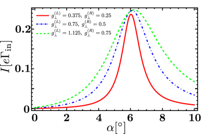
Figure 4: Shape-dependent leakage current in a bent carbon nanotube double quantum dot. The three curves correspond to three different settings of the transverse g factors. By decreasing the transverse g factors, the peak width decreases, i.e., the current becomes more sensitive to the nanotube shape. Parameter values: $B=0.5$ T, $\gamma=0$, $g_{\parallel}=32$, $E_{\tilde{S}}=5\ \mu$eV.

V Conclusion

We studied the dependence of the Pauli-blockade leakage current on the magnetic field direction in a DQD embedded in a bent CNT, and compared our results to a recent experiment. The model we use reproduces a number of previously unexplained experimental features [see (E1)-(E4) of Sec. II]. We demonstrate that the leakage current is sensitive to the shape of the CNT, and this sensitivity increases if the ratio of the longitudinal and transverse g factors increases. In principle, this sensitivity allows for mechanical control of the leakage current, and a characterization of the tube shape via measuring the leakage current. For a recent experiment, we use our model to deduce a deflection angle of 3^∘ from the measured magnetic anisotropy of the leakage current.

Our model does not provide explanation for the weak resonances (E5) seen in the experiment. There are a number of potential future extensions of the present theory: accounting for (i) different longitudinal g-factors in the two dots, (ii) qubit-flip interdot tunneling, (iii) the n-p character of the double dotPei et al. (2012); Li et al. (2014), (iv) valley-mixing character of the electron-electron interactionSecchi and Rontani (2013), (v) Wigner-molecule physicsDeshpande and Bockrath (2008); Wunsch (2009); Secchi and Rontani (2009); von Stecher et al. (2010); Pecker et al. (2013); Secchi and Rontani (2010); Ziani et al. (2013), etc. We believe that incorporating these mechanisms would render the model more accurate quantitatively, and might also allow for an explanation of the observed resonance.