Joint inverse cascade of magnetic energy and magnetic helicity in MHD turbulence

Abstract

We show that oppositely directed fluxes of energy and magnetic helicity coexist in the inertial range in fully developed magnetohydrodynamic (MHD) turbulence with small-scale sources of magnetic helicity. Using a helical shell model of MHD turbulence, we study the high Reynolds number magnetohydrodynamic turbulence for helicity injection at a scale that is much smaller than the scale of energy injection. In a short range of scales larger than the forcing scale of magnetic helicity, a bottleneck-like effect appears, which results in a local reduction of the spectral slope. The slope changes in a domain with a high level of relative magnetic helicity, which determines that part of the magnetic energy related to the helical modes at a given scale. If the relative helicity approaches unity, the spectral slope tends to $-3/2$. We show that this energy pileup is caused by an inverse cascade of magnetic energy associated with the magnetic helicity. This negative energy flux is the contribution of the pure magnetic-to-magnetic energy transfer, which vanishes in the non-helical limit. In the context of astrophysical dynamos, our results indicate that a large-scale dynamo can be affected by the magnetic helicity generated at small scales. The kinetic helicity, in particular, is not involved in the process at all. An interesting finding is that an inverse cascade of magnetic energy can be provided by a small-scale source of magnetic helicity fluctuations without a mean injection of magnetic helicity.

1. Introduction

Magnetohydrodynamic (MHD) turbulence is an important part of astrophysical processes, which gives rise to global cosmic magnetic fields. Over the last few decades, the peculiarities of MHD turbulence have attracted the interest of researchers in astrophysics and fluid dynamics, stimulating numerous theoretical and numerical studies. Recently, significant attention has been paid to the role of magnetic helicity in fully developed MHD turbulence. Magnetic helicity, together with the energy and cross-helicity, is one of the three integrals of motion in ideal MHD, but, compared to energy, the dimensions of helicity have an extra length unit, so magnetic helicity is prone to the inverse cascade and condensation at the largest available scales (Frisch et al., 1975; Biskamp, 1993). The so-called catastrophic quenching problem (Vainshtein & Cattaneo, 1992; Blackman & Field, 2000) is an example of the importance of taking into account the conservation law of magnetic helicity. In consequence, the growth rate of a large-scale magnetic field under large magnetic Reynolds number is predicted to be much less than is required for cosmic dynamos. The transparent boundary and effective transport of the magnetic helicity are usually considered to get rid of the disagreement between theory and astrophysical observations (Brandenburg & Subramanian, 2005). The construction of the corresponding equations is still the subject of discussion (Hubbard & Brandenburg, 2012). Verification of such models might be possible with expected observations of magnetic helicity in real cosmic fields: estimations of magnetic helicity in solar active regions have been performed recently (Zhang et al., 2014; Liu et al., 2014), and there is a possibility that magnetic helicity will be detected in the interstellar medium (Brandenburg & Stepanov, 2014).

The separation of magnetic helicity into the large-scale and small-scale terms is a standard approach in mean-field models of large-scale dynamos, where the effect of turbulence is taken into account through the components of the effective electromotive force (Krause & Rädler, 1980). This separation leads to the problem of correctly estimating of the influx of the magnetic helicity, generated at small (subgrid) scales, into the large scales described by the mean-field equations (Frick et al., 2006). We stress that only the numerical simulations resolving the whole range of scales seem to be capable of highlighting all large-scale dynamo mechanisms.

There are a few reliable results on the spectral transfer of magnetic helicity. The role of magnetic helicity has been studied relatively well in free decaying MHD turbulence. Under free decay, the magnetic helicity of the initial field draws off some of the magnetic field energy in the largest scales. As a result, the energy dissipation follows different scenarios of decay, determined by the initial distribution of the magnetic helicity (Frick & Stepanov, 2010; Brandenburg et al., 2014). Direct numerical simulations (DNS) of statistically stationary turbulence with a substantially helical magnetic field are complicated because they require adequate separation of the forcing scale and dissipation scale for the energy and magnetic helicity. An attempt at this kind of simulations was performed by Alexakis et al. (2006), who showed that the inverse cascade of the magnetic energy and helicity is provided by local interactions during turbulence development and by non-local interactions in the saturated state. However, in this model, the spectral fluxes of magnetic helicity and energy were not separated. The significant direct cascade of magnetic helicity obtained can be explained by the proximity of the dissipation scale to the forcing scale.

Here, we try to highlight the role of magnetic helicity by separating its source from the source of energy. We consider MHD turbulence that is stationary forced at the largest scale, with a source of magnetic helicity that is localized at a scale inside the pronounced inertial range. In our research, we focus on the possibility of a simultaneous direct cascade of energy and oncoming inverse cascade of magnetic helicity, and we examine the influence of the magnetic helicity on the standard Kolmogorov energy cascade. Adding an ad hoc dissipation term at large scale helps to achieve a statistically stationary state. So we deal with the dynamo processes at large Reynolds numbers involving MHD turbulence effects which are of obvious astrophysical interest.

2. Model of MHD turbulence

Studying fully developed turbulent flows demands numerical simulations that clearly resolve the forcing, inertial and dissipation scales. Under a condition of sufficient scale separation, one can produce the universal behavior of turbulent transport of three ideal quadratic invariants known in 3D incompressible magnetohydrodynamics: the total energy $E=\langle|{\bf u}|^{2}+|{\bf b}|^{2}\rangle/2$, the cross-helicity $H^{c}=\langle{\bf u}\cdot{\bf b}\rangle$ and the magnetic helicity $H^{b}=\langle{\bf a}\cdot{\bf b}\rangle$, where ${\bf u}$ is the velocity field, ${\bf b}$ is the magnetic field, ${\bf a}$ is the vector potential (${\bf b}={\rm\nabla}\times{\bf a}$) and $\langle.\rangle$ means volume averaging. However, even recent direct numerical simulations using billions of grid points hardly provided an inertial range of scales wider than one decade (Mininni & Pouquet, 2007). This is the reason we turn to the shell models of turbulence. These models cannot take into account the spatial complexity of turbulent flows but reflect such properties of real MHD turbulence as spectral distributions, intermittency and chaotic reversals of large-scale modes (see, e.g. Plunian et al. (2013)). Furthermore, these models produce an extended inertial range and accurate dissipation rate using realistic values for the governing parameters (high kinetic and magnetic Reynolds numbers, low or high magnetic Prandtl number).

Shell models are low-dimensional dynamic systems that are derived from the original MHD equations by a drastic reduction of the number of variables. These models describe the dynamics and spectral distributions of fully developed MHD turbulence through a set of complex variables $U_{n}$, $B_{n}$, which characterize the kinetic energy $E_{n}^{u}=|U_{n}|^{2}/2$ and magnetic energy $E_{n}^{b}=|B_{n}|^{2}/2$ of pulsations in the wave number range $k_{n}<|{\bf k}|<k_{n+1}$ (called the shell $n$), where $k_{n}=\lambda^{n}$ ($\lambda$ is the shell width in a logarithmic scale, typically chosen to be equal 1.618). Model equations are

$$d_{t}U_{n}={W_{n}}({\bf U},{\bf U})-{W_{n}}({\bf B},{\bf B})-k_{n}^{2}\frac{U_{n}}{{\rm Re}}+F_{n},\phantom{XX}$$ (1)

$$d_{t}B_{n}={W_{n}}({\bf U},{\bf B})-{W_{n}}({\bf B},{\bf U})-k_{n}^{2}\frac{B_{n}}{{\rm Rm}}+G_{n}-D_{n},$$

where ${\rm Re}$ and ${\rm Rm}$ are the kinetic and magnetic Reynolds numbers, ${\bf U}=(U_{0},...U_{N-1})$ and ${\bf B}=(B_{0},...B_{N-1})$ are vectors in space $\mathbb{C}^{N}$, and $N$ is the total number of shells. The structure of equations (1) mimics the original MHD equations – the bilinear form ${\bf W}({\bf X},{\bf Y})$ is like ${\bf X}\cdot\nabla{\bf Y}$ and terms $F_{n}$, $G_{n}$ and $D_{n}$ specify external forces acting in the shell $n$. We use the $W_{n}({\bf X},{\bf Y})$ suggested by Mizeva et al. (2009), which can be rewritten in a general form as

$$W_{n}({\bf X},{\bf Y})=ik_{n}[(X_{n-1}Y_{n-1}+X_{n-1}^{*}Y_{n-1}^{*})-\lambda X_{n}^{*}Y_{n+1}^{*}$$

$$-\frac{\lambda^{2}}{2}(X_{n}Y_{n+1}+X_{n+1}Y_{n}+X_{n}Y_{n+1}^{*}+X^{*}_{n+1}Y_{n})$$

$$-\frac{\lambda}{2}(X_{n-1}^{*}Y_{n-1}-X_{n-1}Y_{n-1}^{*})+\lambda X^{*}Y_{n+1}]$$

$$-ik_{n}\lambda^{-5/2}[\frac{1}{2}(X_{n-1}Y_{n}+X_{n}Y_{n-1})+\lambda X^{*}_{n}Y_{n-1}^{*}$$

$$-\lambda^{2}(X_{n+1}Y_{n+1}+X_{n+1}^{*}Y_{n+1}^{*})+\frac{1}{2}(X_{n}Y_{n-1}^{*}+X_{n-1}^{*}Y_{n})$$

$$-\lambda X^{*}_{n}Y_{n-1}+\frac{\lambda}{2}(X_{n+1}^{*}Y_{n+1}-X_{n+1}Y_{n+1}^{*})].\phantom{XX}$$ (2)

In the non-dissipative limit, equations (1) conserve the total energy $E=\sum(E^{u}_{n}+E^{b}_{n})$, the cross-helicity $H^{c}=\sum(U_{n}B_{n}^{*}+B_{n}U_{n}^{*})/2$ and the magnetic helicity $H^{b}=\sum\imath k_{n}^{-1}((B_{n}^{*})^{2}-B_{n}^{2})/2$. For a comprehensive review of MHD shell models, refer to Plunian et al. (2013).

The key point of our modelling is a particular forcing design to create stationary cascades. We excite the turbulence in the classical way by injecting kinetic energy at the largest scale. Namely, we take $F_{n}$ at $n=0$ ($k=1$) only, in the form

$$F_{0}=I_{f}\exp(\imath\phi)$$ (3)

where $I_{f}$ is constant and $\phi$ is a random phase that remains constant during each time interval $t_{c}$. Then, the time-averaged energy injection rate becomes $\varepsilon=I_{f}^{2}t_{c}$, and the injection rates of the kinetic helicity and cross-helicity vanish under the condition that $t_{c}$ is shorter than the large-scale turnover time.

The magnetic forces $G_{n}$ and $D_{n}$ are introduced to simulate the source and sink of magnetic helicity, acting at shells $n_{g}$ and $n_{d}$, respectively. For magnetic helicity injection, the force is taken as

$$G_{n}=\frac{\imath I_{g}k_{n}B_{n}(B_{n}^{2}+(B_{n}^{*})^{2})}{16(E_{n}^{b})^{2}}$$ (4)

with $n=n_{g}$. Then, the injection rate for magnetic helicity is $\chi=I_{g}(1-(H_{n}^{r})^{2})$, where $H_{n}^{r}=k_{n}H_{n}^{b}/(2E_{n}^{b})$ is the relative magnetic helicity. We note here that the force (4) does not change the magnetic energy and becomes zero for marginal values $H^{r}_{n}=\pm 1$.

To produce an stationary inverse cascade of magnetic helicity and avoid its accumulation at the largest scale, we introduce a large-scale sink of the magnetic helicity as an additional dissipation

$$D_{n}=\frac{I_{d}k_{n}^{2}B_{n}(H_{n}^{b})^{2}}{8(E_{n}^{b})^{3}},$$ (5)

with $n=n_{d}$. This gives magnetic energy dissipation with a rate $\varepsilon_{d}=I_{d}(H_{n}^{r})^{2}$ and magnetic helicity dissipation with a rate $\chi_{d}=2I_{d}k_{n}^{-1}(H_{n}^{r})^{3}$. In the non-helical case ($H_{n}^{r}\to 0$), this dissipation tends to zero. The force (5) imitate in the shell model the real open boundary condition typical for astrophysical objects with cosmic magnetic field.

3. Results

Our reference case of simulations is stationary forced MHD turbulence without injection of magnetic helicity. We numerically evolve Equations (1) for ${\rm Re}={\rm Rm}=10^{6}$ and use amplitude $I_{f}=10$ and $t_{c}=0.01$ for the force (3), which provides the energy injection rate $\varepsilon=1$ at the scale $k=1$. The corresponding spectrum and spectral flux of the total energy are shown in Figure 1. All curves corresponding to this non-helical case are shown in black. A Kolmogorov’s spectral law $E\sim k^{-5/3}$ (which corresponds to $E_{n}\sim k_{n}^{-2/3}$) and a flat spectral flux extend for about three decades. The shell models gain an advantage over DNS with this considerable separation of forcing and dissipation scales. Note, that all statistical quantities shown in our figures are calculated by averaging over 32 numerical realizations, performed for similar initial conditions each for a period of $10^{3}$ large-scale turnover times.

(a)

(b)

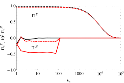
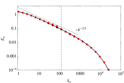
Figure 1.— Spectral fluxes (a) and spectra (b) of the total energy for stationary forced MHD turbulence. Black lines correspond to the non-helical case. Red lines show the spectrum and fluxes for magnetic helicity injection at wave number $k_{g}=122$ indicated by a vertical dashed line. The spectral fluxes of the total energy $\Pi^{E}_{n}$ are shown by a dotted lines. The spectral fluxes of the magnetic helicity $\Pi^{H}_{n}$ multiplied by a factor $10^{2}$ are shown for three injection rates: $I_{g}=0$ (black solid), $I_{g}=0.05$ (red dashed) and $I_{g}=0.5$ (red solid). The thin straight line corresponds to the Kolmogorov’s slope.

Next we consider a helical case with an injection of magnetic helicity within the inertial range, namely at $k_{g}=122$ ($n_{g}=10$), with a constant mean injection rate $\chi>0$ provided by the force (4). The injected magnetic helicity is transferred toward scales larger than $k_{g}$. This means that the magnetic helicity spectral flux $\Pi^{H}_{n}$ is negative. To achieve the stationary state of turbulence, we remove the magnetic helicity at $k=1$ ($n_{d}=0$) using force (5) with $I_{d}=1$. This value of $I_{d}$ is sufficient to keep balance of the injection and dissipation rates of magnetic helicity $\chi=\chi_{d}$ for any $I_{g}$. Figure 1(a) shows a stable inverse cascade of magnetic helicity with almost constant spectral flux $\Pi^{H}_{n}$ for different values of $I_{g}$, which do not noticeably influence the direct cascade of energy characterized by positive energy flux $\Pi^{E}_{n}$. Figure 1(b) shows that the helicity injection does not change the energy spectrum, except for a small bump near $k_{g}$.

To emphasis the bump, we present in Figure 2(a) the compensated spectra of the total, kinetic and magnetic energies separately for the helical case. The non-helical spectrum is close to horizontal, which corresponds to Kolmogorov’s power law with exponent $-5/3$. Increasing $I_{g}$ leads to an increase of $\Pi^{H}_{n}$ and to the growth of relative magnetic helicity $H^{r}_{n}=kH^{b}_{n}/2E^{b}_{n}$ over the whole spectrum, as is shown in Figure 2(b). However, a more intensive injection than $I_{g}=0.5$ does not change the situation because $H^{r}_{n}$ reaches the limit equal to unity and the forcing is saturated. In this saturated state, the spectral slope at wave numbers smaller than $k_{g}$ tends to the $-3/2$ power law. Recall that there is energy injection at $k_{g}$ and the corresponding scale is rather far from the energy forcing scale and the dissipation scale. The physics behind this bump should be explained by local distortion caused by pure magnetic helicity injection.

(a)

(b)

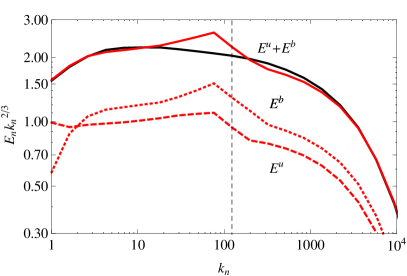
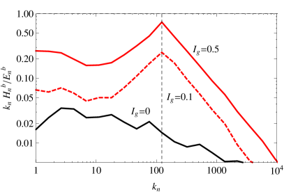
Figure 2.— (a) Compensated spectra of energy (kinetic, magnetic and total) together with the spectrum of total energy for the non-helical case (black line). (b) Spectra of relative magnetic helicity $H^{r}_{n}$ for $I_{g}=0$ (black line), $I_{g}=0.1$ (red dashed line) and $I_{g}=0.5$ (red solid line).

A kind of pileup of the energy spectrum in the inertial range is known for conventional developed turbulence as a result of the bottleneck phenomenon (Falkovich, 1994). In isotropic fully developed hydrodynamic turbulence, the bottleneck effect is caused by edge effects, related to the transition from inertial to diffusive scales. The viscous suppression of small-scale modes removes some triads from non-linear interaction and makes the spectral energy transfer less efficient, which leads to a pileup of energy at the end of the inertial range of scales. Note that in shell models this effect could be reproduced by using a non-local model that includes interactions of remote shells (Plunian & Stepanov, 2007).

(a)

(b)

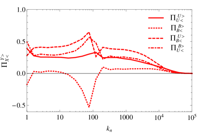
Figure 3.— Four components of the energy flux $\Pi_{U^{<}}^{U^{>}}$, $\Pi_{U^{<}}^{B^{>}}$, $\Pi_{B^{<}}^{U^{>}}$ and $\Pi_{B^{<}}^{B^{>}}$ vs the wave number $k_{n}$ for the non-helical case $I_{g}=0$ (a) and helical case $I_{g}=0.5$ (b).

We suggest that the effect of the magnetic helicity on the energy spectrum could be clarified by considering energy transfers between kinetic and magnetic field modes of different scales. Shell-to-shell energy transfer in magnetohydrodynamics has been suggested and considered in frame of DNS by Alexakis et al. (2005). An analogous formalism had been derived in terms of shell models (Plunian & Stepanov, 2007). Instead of shell-to-shell transfers, we prefer to use the spectral fluxes as defined by Lessinnes et al. (2009):

$$\Pi_{U^{<}}^{U^{>}}=-{\bf W}({\bf U},{\bf U})\cdot{\bf U}_{n}^{<},$$

$$\Pi_{U^{<}}^{B^{>}}=-{\bf W}({\bf B},{\bf B})\cdot{\bf U}_{n}^{<},$$ (6)

$$\Pi_{B^{<}}^{B^{>}}={\bf W}({\bf U},{\bf B}_{n}^{>})\cdot{\bf B}_{n}^{<},$$

$$\Pi_{B^{<}}^{U^{>}}=-{\bf W}({\bf B},{\bf U}_{n}^{>})\cdot{\bf B}_{n}^{<},$$

where each $\Pi_{X^{<}}^{Y^{>}}$ denotes the spectral energy flux from ${\bf X}_{n}^{<}=(X_{1},X_{2},...X_{n},0,\dots)$ to ${\bf Y}_{n}^{>}=(0,...Y_{n+1},Y_{n+2},...)$. In the flux notation the subscripts $n$ has been dropped for convenience, e.g. $\Pi_{X^{<}}^{Y^{>}}$ is a function of $n$ and must be understood as $\Pi_{X_{n}^{<}}^{Y_{n}^{>}}$. Definitions (6) satisfy the total energy conservation condition so that

$$\Pi^{E}=\Pi_{U^{<}}^{U^{>}}+\Pi_{U^{<}}^{B^{>}}+\Pi_{B^{<}}^{B^{>}}+\Pi_{B^{<}}^{U^{>}}.$$

Figure 3 shows these four components of the energy flux (6) for the non-helical and helical cases. For non-helical turbulence (see Figure 3(a)) the term $\Pi_{B^{<}}^{B^{>}}$ is negligible with respect to other three, which are constant over the inertial range. Injection of the magnetic helicity results in the negative flux $\Pi_{B^{<}}^{B^{>}}$ (see Figure 3(b)). $\Pi_{B^{<}}^{B^{>}}$ has a minimum near $k_{g}$ and scales as $\Pi_{B^{<}}^{B^{>}}\sim\Pi^{H}k$ for $k\leq k_{g}$. Thus the flux of magnetic helicity is necessary associated with the inverse flux of magnetic energy, that is described by $\Pi_{B^{<}}^{B^{>}}$. Since the total energy flux through any wave number inside the inertial range must be constant, fluxes $\Pi_{U^{<}}^{U^{>}}$, $\Pi_{U^{<}}^{B^{>}}$ and $\Pi_{B^{<}}^{U^{>}}$ compensate for the drop caused by $\Pi_{B^{<}}^{B^{>}}$. One can see the corresponding growth of these fluxes at $k_{g}$ in Figure 3(b). This growth is provided by intensification of the kinetic and magnetic fields near $k_{g}$. As a consequence, a bump forms in the energy spectrum.

Note that all the above results were obtained for positive $I_{g}$, which provide an injection of positive magnetic helicity only. Changing of the sign does not affect the results, except for the sign of the magnetic helicity spectral flux. $\Pi^{H}_{n}$ for $k<k_{g}$ becomes positive corresponding to an inverse (negative) cascade of negative helicity.

Finally we address the question of what happens if the small-scale source of magnetic helicity produces a fluctuating magnetic helicity injection, being zero averaged over time. To examine this case, we introduce a force that injects magnetic helicity in an alternating manner. Namely the sign of the injected helicity corresponds to the actual value of magnetic helicity. This can be done by modifying force (4) via multiplying by $H^{r}_{n}$ so that

$$G_{n}=\frac{\imath I_{g}k_{n}^{2}B_{n}H_{n}^{b}(B_{n}^{2}+(B_{n}^{*})^{2})}{(E_{n}^{b})^{3}}.$$ (7)

The injection rate, caused by this force, is $\chi=16I_{g}(1-(H_{n}^{r})^{2})H^{r}_{n}$. The resulting energy spectrum and magnetic helicity flux are shown in Figure 4(a). One can see that the effect is similar to that obtained with the force (4), which injects magnetic helicity of fixed sign. The particularity of the result is that the averaged helicity spectrum (see Figure 4(b)) does not differ from the spectrum for the non-helical case (compare black and red curves). As expected, the force (7) just amplifies the amplitude of the magnetic helicity fluctuation and increases the characteristic time between the changes in its sign. The time during which the magnetic helicity has the same sign becomes sufficient to initiate the inverse cascade. Recall that injected negative helicity cascades to large scales under a positive spectral flux. However, the flux $\Pi_{B^{<}}^{B^{>}}$ is negative anyway. So we have found a situation in which any characteristics of the magnetic helicity does not reveal the inverse cascade (the spectral distribution of both magnetic helicity and its flux do not change), while the associated flux of magnetic energy can be detected, namely by the contribution to the energy flux, provided by the term $\Pi_{B^{<}}^{B^{>}}$.

(a)

(b)

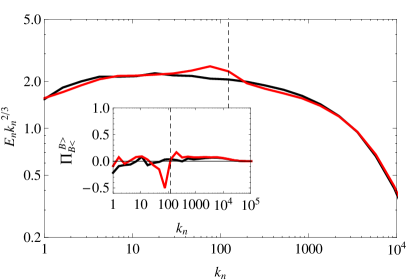
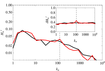
Figure 4.— The case with an alternating injection of magnetic helicity: (a) compensated spectra (the inset is the magnetic-to-magnetic energy flux) and (b) relative magnetic helicity (the inset shows the standard deviation of $H^{r}_{n}$. $I_{g}=0$ - black curves, $I_{g}=1$ - red curves.

4. Conclusions

In fully developed MHD turbulence, a source of magnetic helicity at small scale provides a negative spectral flux, which coexists with the direct energy flux in the inertial range. Near the scale of helicity injection a bottleneck-like effect appears, which leads to a local reduction of the spectral slope. We found that the key quantity for understanding this effect is the magnetic-to-magnetic energy spectral flux. This flux, being negligible in the non-helical case, is negative and clearly associated with an inverse cascade of magnetic helicity independent of the sign of the injected helicity. The same effect can be obtained even for an alternating source of small-scale magnetic helicity with a zero-mean injection rate. In spite of the rather special conditions in our modelling, a similar scenario to some extend can develop in realistic situations, e.g. magnetic helicity injection into the corona in emerging active regions (Liu et al., 2014).

The physical implications of the simulations presented in the paper are the following reasoning about the large-scale dynamo mechanism. Mirror symmetry breaking of magnetic field fluctuations at small scales initiates an inverse cascade of magnetic helicity. This leads necessarily to a magnetic energy spectral flux from small scales to large scales, which consequently causes the growth of a large-scale magnetic field in the kinematic dynamo regime. The large-scale magnetic energy becomes saturated when the inverse spectral fluxes of the magnetic energy and helicity are compensated by corresponding outflows at the largest scale. Figure 5 shows that the reduction of a large-scale dissipative force (5) results in accumulation of magnetic energy at large scales. We believe that this qualitative scenario was implicitly assumed in earlier studies. However, we have succeeded in demonstrating the scenario for the developed MHD turbulence, with an extended inertial range, using a model based on local interactions of scales. We note that mixing of local and nonlocal interactions is not avoidable even in the recent large-scale dynamo simulations due to a lack of resolution. Actually, we have posed the problem of the realisability of a large-scale dynamo in terms of the efficiency of mode interactions, which provide a magnetic-to-magnetic inverse energy spectral flux and emphatically recommend this for consideration. In addition, we have found that the magnetic helicity injection in the alternating manner (being zero averaged in time) plays the same role.

Figure 5.— Spectra of magnetic energy (the inset is the compensated version) the magnetic-to-magnetic energy flux) for $I_{g}=0.5$ and different amplitude of the dissipative force (5): $I_{d}=1$ (solid line), $I_{d}=0.4$ (dashed line) and $I_{d}=0.1$ ( dotted line).

Apparently the mechanism considered for the magnetic energy condensation at large scale can be interpreted as the fluctuating magnetic $\alpha$-effect, which allows the large-scale dynamo to persist at values of the Reynolds numbers relevant for astrophysical conditions. In contrast to the dynamo recently suggested by Tobias & Cattaneo (2013), which was also obtained for a large-scale magnetic field at large ${\rm Rm}$, our dynamo model does not contain any shear-like terms nor kinetic helicity forcing.

The result obtained is important for the theory of astrophysical dynamos, showing that a large-scale dynamo can be affected by the magnetic helicity generated at small scales. In particular, it means that for mean-field dynamo models one should consider the possible flux of magnetic helicity from small (subgrid) scales. Note, that this contribution by small-scale turbulence for a large-scale dynamo can be described by multi-scale models, which use mean-field equations for the large scales and shell equations for the small scales (Frick et al., 2006; Nigro & Veltri, 2011).

References

- Alexakis et al. (2005) Alexakis, A., Mininni, P. D., & Pouquet, A. 2005, Phys. Rev. E, 72, 046301
- Alexakis et al. (2006) Alexakis, A., Mininni, P. D., & Pouquet, A. 2006, ApJ, 640, 335
- Biskamp (1993) Biskamp, D. 1993, Nonlinear magnetohydrodynamics (Cambridge Monographs on Plasma Physics)
- Blackman & Field (2000) Blackman, E. G., & Field, G. B. 2000, ApJ, 534, 984
- Brandenburg et al. (2014) Brandenburg, A., Kahniashvili, T., & Tevzadze, A. G. 2014, ArXiv e-prints, arXiv:1404.2238
- Brandenburg & Stepanov (2014) Brandenburg, A., & Stepanov, R. 2014, ApJ, 786, 91
- Brandenburg & Subramanian (2005) Brandenburg, A., & Subramanian, K. 2005, Phys. Rep., 417, 1
- Falkovich (1994) Falkovich, G. 1994, Physics of Fluids, 6, 1411
- Frick & Stepanov (2010) Frick, P., & Stepanov, R. 2010, Europhys. Lett., 92, 34007
- Frick et al. (2006) Frick, P., Stepanov, R., & Sokoloff, D. 2006, Phys. Rev. E, 74, 066310
- Frisch et al. (1975) Frisch, U., Pouquet, A., Leorat, J., & Mazure, A. 1975, J. Fluid Mech., 68, 769
- Hubbard & Brandenburg (2012) Hubbard, A., & Brandenburg, A. 2012, ApJ, 748, 51
- Krause & Rädler (1980) Krause, F., & Rädler, K.-H. 1980, Mean-field magnetos and dynamo theory (Akademie-Verlag Berlin)
- Lessinnes et al. (2009) Lessinnes, T., Carati, D., & Verma, M. K. 2009, Phys. Rev. E, 79, 066307
- Liu et al. (2014) Liu, Y., Hoeksema, J. T., Bobra, M., et al. 2014, ApJ, 785, 13
- Mininni & Pouquet (2007) Mininni, P. D., & Pouquet, A. 2007, Phys. Rev. Lett., 99, 254502
- Mizeva et al. (2009) Mizeva, I. A., Stepanov, R. A., & Frik, P. G. 2009, Physics - Doklady, 54, 93
- Nigro & Veltri (2011) Nigro, G., & Veltri, P. 2011, ApJ, 740, L37
- Plunian & Stepanov (2007) Plunian, F., & Stepanov, R. 2007, New J. Phys., 9, 294
- Plunian et al. (2013) Plunian, F., Stepanov, R., & Frick, P. 2013, Phys. Rep., 523, 1
- Tobias & Cattaneo (2013) Tobias, S. M., & Cattaneo, F. 2013, Nature, 497, 463
- Vainshtein & Cattaneo (1992) Vainshtein, S. I., & Cattaneo, F. 1992, ApJ, 393, 165
- Zhang et al. (2014) Zhang, H., Brandenburg, A., & Sokoloff, D. D. 2014, ApJ, 784, L45