Sequential Hypothesis Tests for Adaptive Locality Sensitive Hashing
Abstract
All pairs similarity search is a problem where a set of data objects is given and the task is to find all pairs of objects that have similarity above a certain threshold for a given similarity measure-of-interest. When the number of points or dimensionality is high, standard solutions fail to scale gracefully. Approximate solutions such as Locality Sensitive Hashing (LSH) and its Bayesian variants (BayesLSH and BayesLSHLite) alleviate the problem to some extent and provides substantial speedup over traditional index based approaches. BayesLSH is used for pruning the candidate space and computation of approximate similarity, whereas BayesLSHLite can only prune the candidates, but similarity needs to be computed exactly on the original data. Thus where ever the explicit data representation is available and exact similarity computation is not too expensive, BayesLSHLite can be used to aggressively prune candidates and provide substantial speedup without losing too much on quality. However, the loss in quality is higher in the BayesLSH variant, where explicit data representation is not available, rather only a hash sketch is available and similarity has to be estimated approximately. In this work we revisit the LSH problem from a Frequentist setting and formulate sequential tests for composite hypothesis (similarity greater than or less than threshold) that can be leveraged by such LSH algorithms for adaptively pruning candidates aggressively. We propose a vanilla sequential probability ration test (SPRT) approach based on this idea and two novel variants. We extend these variants to the case where approximate similarity needs to be computed using fixed-width sequential confidence interval generation technique. We compare these novel variants with the SPRT variant and BayesLSH/BayesLSHLite variants and show that they can provide tighter qualitative guarantees over BayesLSH/BayesLSHLite – a state-of-the-art approach – while being upto 2.1x faster than a traditional SPRT and 8.8x faster than AllPairs.
1 Introduction
Similarity search in a collection of objects has a wide variety of applications such as clustering [16], semi-supervised learning [22], information retrieval [5], query refinement on websearch [1], near duplicate detection [21], collaborative filtering, and link prediction [14]. Formally, the problem statement is: Given a collection of objects D and an associated similarity measure and a similarity threshold , the problem is to find all pairs of objects , such that , where .
The major challenge in most of these areas is dealing with a large volume of the data. The volume combined with the high dimensionality of the datasets can lead to inefficient solutions to this problem. Recent research has focused on reducing the candidate search space. The AllPairs [1] candidate generation algorithm builds a smart index structure from the vector representation of the points to give the exact similarity. Another approach is to do an approximate similarity calculation which involves sacrificing small accuracy for substantial speedup. The most popular technique is the locality sensitive hashing(LSH) [10, 7] which involves projecting the high dimensional data into a lower dimensional space and similarity of a pair of points is approximated by the number of matching attributes in the low dimensional space.
A recent idea, BayesLSHLite technique [18], further aggressively prunes the candidate space to generate the set of pairs above the user-defined similarity threshold efficiently. The way BayesLSHLite works is, for a pair of data objects , BayesLSHLite incrementally compares their hashes (in batches of size ) and infers after each batch, how likely is it that pair will have similarity above the threshold. As the name suggests it relies on Bayesian principles and priors for making the adaptive decision to prune or retain a candidate. If that probability becomes too low, then candidate pair is pruned away. The above algorithm has a variant called BayesLSH, where after the candidate pruning is done, similarity is estimated approximately from the hash signatures instead of exact computation. This is useful in cases where exact similarity computation is infeasible. Exact similarity computation might be infeasible in cases where the original data was too large too store and the small hash sketch of the data was stored instead. Another scenario could be where the similarity measure-of-interest is a kernel function and exact representation of the data points in the kernel induced feature space is not possible as that space might be infinite dimensional (e.g. Gaussian RBF kernel). Additionally, the specialized kernel functions are extremely expensive to compute on the fly. In such cases, both candidate generation and similarity estimation has to be done approximately using the LSH hash sketches.
In this paper we adapt a Frequentist view of this idea and propose a fully principled sequential model to do the incremental pruning task with rigorous quality guarantees. Specifically, we model the problem of as a sequential hypothesis test problem and provide quality guarantees through Type I and Type II errors. We start with the traditional SPRT [19], and show that it is extremely inefficient in practice, making it unsuitable for large scale analytics. We then propose an alternate sequential hypothesis test procedure based on a one-sided fixed-width confidence limit construction technique. Finally we show that no single hypothesis testing strategy works well for all similarity values. Therefore, we propose a fine-grained hybrid hypothesis testing strategy, which based on a crude estimate of the similarity from the first batch of hash comparisons for that specific candidate pair, selects the most suitable test for that pair. In other words, instead of using a single hypothesis test, we dynamically choose the best suited hypothesis test for each candidate pair. We extend the above to technique to develop a variant, that after candidate pruning, estimates the approximate similarity by using the fixed-width two-sided confidence interval generation technique [6]. Our ideas are simple to implement and we show that our hybrid method always guarantees the minimum quality requirement (as specified by parameters input to the algorithm), while being upto 2.1x faster than an SPRT-based approach and 8.8x faster than AllPairs while qualitatively improving on the state-of-the-art BayesLSH/Lite estimates.
2 Background
2.1 Locality Sensitive Hashing
Locality sensitive hashing[10, 7] is a popular and fast method for candidate generation and approximate similarity computation within a large high dimensional dataset. Research has demonstrated how to leverage the key principles for a host of distance and similarity measures [10, 4, 2, 16, 9]. Briefly, each data point is represented by a set of hash keys using a specific hash family for a given distance or similarity measure (). Such a family hash function is said to have the locality sensitive hashing property if:
| (1) |
where are the any two points in the dataset, and is a randomly selected hash function from within a family of hash functions. Consequently, the approximate similarity between the pair can be estimated as:
where is the total number of hash functions.
2.2 Candidate generation
We use the AllPairs [1] candidate generation algorithm when the original data set is available. The AllPairs candidate generation algorithm is exact, hence all true positives (candidates with similarity above the threshold) will be present in the set of candidates generated. The AllPairs algorithm builds an index from vector representation of the data and instead of building a full inverted index, AllPairs only indexes the information which may lead to a pair having similarity greater than the specified threshold. The AllPairs algorithm can be used when the original dataset is small enough to be stored entirely and the similarity of interest is computed on the original feature space (unlike kernel similarity measures).
In cases where the entire dataset cannot be stored, rather a small sketch of it is available, AllPairs cannot be used. Additionally if the similarity is a form of kernel measure and the feature space of that kernel cannot be explicitely represented, AllPairs will not work as it relies on the explicit representation of the data points. However, in both scenarios we can use LSH to generate a low dimensional sketch of the dataset and use the following probabilistic candidate generation algorithm. We follow the general index structure for LSH candidate generation used in [10, 4, 2, 16, 9]. The advantage of such an index structure is that the number of candidates to search for a certain point too see which of them has higher similarity than a threshold becomes much less compared to exhaustive search. That is search can be be done in sublinear time. LSH based index structures perform well compared to traditional indices when the dimensionality of the data set is very high. The algorithm is as follows:
-
1.
Using a locality sensitive hashing method for a given similarity measure, form signatures for each data point, each signature having hash keys.
-
2.
Each pair of points, that share at least one signature will stay in the same hash bucket.
-
3.
During all pairs similarity search, for each point, only those points which are in the same bucket needs to be searched.
-
4.
From [21], for a given and similarity threshold , the number of signatures required for a recall ,
2.3 Candidate Pruning using BayesLSH/Lite
Traditionally maximum likelihood estimators are used to approximate similarity of a pair to decide whether it is above or below a certain threshold. For a candidate pair, if there are a total of hashes and of them match, then the similarity estimate is . The variance of this estimator is where is the similarity between the candiate pair. Two issues to observe here are - 1) as increases, the variance decreases and hence the accuracy of the estimator increases, 2) more importantly, the variance of the estimator depends on the similarity of the pair itself. This means for a fixed number of hashes, the accuracy achieved if the similarity of the candidate pair was 0.9 is higher than if the similarity was 0.5. In other words the number of hashes required for different candidate pairs for achieving the same level of accuracy is different. Therefore, the problem with fixing the number of hashes is - some of the candidate pairs can be pruned by comparing the first few hashes only. For example if the similarity threshold is 0.9 and 8 out of the first 10 hashes did not match, there is very low probability that the similarity of the pair is greater than 0.9. The BayesLSH/Lite[18] is among the earliest approaches to solve this problem of deciding the number of hash comparisons. Instead it incrementally compares hashes until the candidate pair can be pruned with a certain probability, or the maximum allowed hash comparisons is reached. It will then compute exact or approximate similarity to make the decision. To do the incremental pruning, BayesLSHLite solves the inference problem , where is the similarity threshold. Additionally, the BayesLSH variant estimates the approximate similarity by creating an interval for the true similarity by the solving the inference . Both inferences are solved using a simple Bayesian model. These inferences help overcome the second problem pointed above - number of hashes required to prune a candidate or build an interval around it adaptively set for each candidate pair.
Since we are counting the number of matches out of hash comparison, and each comparison is independent with match probability as per equation 1, the likelihood function becomes a binomial distribution with parameters and . If is the random variable denoting matches out of hash bit comparisons, and let be the similarity , then the likelihood function will be:
| (2) |
In the Bayesian setting, the parameter can be treated as a random variable. Let the estimate of in this setting be . Using the aforementioned likelihood function, the two inference problems become:
Early pruning inference: given m matches out of n bits, what is the probability that the similarity is above threshold :
| (3) |
Concentration inference: given the similarity estimate , what is the probability that it falls within of the true similarity:
| (4) | |||||
The BayesLSHLite algorithm works as follows:
For each pair x,y:
-
1.
Compare the next hashes and compute the early pruning probability .
-
2.
If , then prune the pair and stop.
-
3.
If maximum allowable hash comparisons have been reached, compute exact similarity and stop.
-
4.
Go to step 1.
The BayesLSH variant works as follows:
For each pair x,y:
-
1.
Compare the next hashes and compute the early pruning probability .
-
2.
If , then prune the pair and stop.
-
3.
If , then output pair if and stop.
-
4.
If maximum allowable hash comparisons have been reached, then output pair if and stop.
-
5.
Go to step 1.
3 Case for Frequentist Formulation
The BayesLSHLite candidate pruning algorithm and the BayesLSH approximate similarity estimation algorithm as described in the previous section, provides the basis for the current work. Specifically in this work we examine the same problems they attempt to solve but in a Frequentist setting. We note that the inferences (equations 3 and 4) in the above BayesLSH/Lite algorithms is done every hash comparisons (this can be viewed as a bin of comparisons). Therefore, for a candidate pair, if the pruning inference is done once, then the error probability rate will , but when it is done for the second time, probability of the pair getting pruned will be determined by getting pruned the first time (first bin) and the probability of getting pruned the second time (a cumulative of the first and second bin matches). Essentially, we argue in this work that this error rate may propogate resulting in an accumulated error over multiple pruning inferences. The underlying reason is, BayesLSHLite tries to model an inherently sequential decision process in a non-sequential way. The same scenario is true for the concentration inference as well (equation 4). Over multiple concentration inferences done incrementally, the coverage probability could fall below . We note that in practice this may not be a significant issue but the question remains can this problem be fixed (in the rare cases it may materialize) without significantly impacting the gains obtained by BayesLSH/Lite. We note that fixing this problem in a Bayesian setting remains open but in this work we show how this problem can be fixed in a Frequentist setting.
Another issue, again a minor one, is when a pair is unlikely to be above a certain similarity threshold, pruning it early saves hash comparisons, similarly when a pair is very likely to be above the threshold, hash comparison for it should stop immediately and it should be processed for exact similarity computation. This can also save a number of hash comparisons.
To overcome these problems, we propose to model the problem in a Frequentist setting as follows. In the frequentist setting let the similarity be denoted by the parameter (intead of S as in Bayesian setting).
-
•
We model the early pruning inference as a sequential hypothesis test problem that should be able to guarantee Type I and Type II errors under the sequential hash comparison setting and if possible, it should be able to early prune a pair or send a pair for exact similarity computation.
-
•
We model the concentration inference as a sequential two-sided fixed-width confidence interval creation problem that should be able to guarantee a certain coverage probability.
4 Methodology
In this section, we describe a principled way of doing the early pruning inference (equation 3) and a principled way of doing the concentration inference (equation 4) under the sequential setting where the number of hash functions () is not fixed, rather it is also a random variable.
4.1 Early Pruning Inference
We use sequential tests of composite hypothesis for pruning the number of the generated candidates, so that the cardinality of the remaining candidate set is very small. Therefore, exact similarity computation on the remaining set of candidate pairs becomes feasible in terms of execution time, provided the original data set is available and the similarity function can be computed on the feature space of the original data. Our pruning algorithm involves sequentially comparing the hashes for a pair of data objects and stop when we are able to infer with some certainty whether the similarity for the pair is above or below the user defined threshold. If, according to the inference, the similarity of the pair is below the threshold, then we prune away the pair, otherwise we compute exact or approximate similarity of the pair depending on which variant we are using. More formally, if the similarity of the pair is and the user defined threshold is , we need to solve the hypothesis test, where the null hypothesis is and the alternate hypothesis is . Two interesting aspects of our problem formulation are:
-
1.
For performance reasons as described in section 3, we do not want to fix the number of hashes to compare for the hypothesis test, but rather incrementally compare the hashes and stop when a certain accuracy in terms of Type I error has been achieved.
-
2.
We focus on Type I error, i.e. we do not want to prune away candidate pairs which are true positives (). We can allow false positives () in our final set, as either exact similarity computation or approximate similarity estimation will be done on the final set of candidate pairs and any false positives can thus be pruned away. In other words, we do not need to provide guarantees on Type II error of the hypothesis test. Ofcourse keeping a low Type II error implies less false positives to process, resulting in better performance.
We discuss three strategies for formulating the hypothesis test. First, we cast our problem in a traditional Sequential Probability Ratio Test (SPRT) [19] setting and then discuss the shortcomings of such an approach. Second, we then develop a sequential hypothesis test based on a sequential fixed width one-sided confidence interval (CI) and show how it can overcome some of the limitations of traditional SPRT. We empirically find that even this test does not always perform better than the more traditional SPRT. Third, building on the above, we propose a hybrid approach (HYB), where we dynamically select the hypothesis test (SPRT or CI) based on the similarity of each candidate pair which we crudely estimate from the first few comparisons. In other words, instead of using a single fixed hypothesis test, we select one which is best suited for the candidate pair being estimated.
For a candidate pair with similarity , the probability of a hash matching is for a locality sensitive hash function as described in equation 1. Therefore, given hashes for the pair, the probability that of them will match follows a binomial distribution with parameters and . This is because the individual hash matching probabilities are identically and independently distributed Bernoulli with parameter . So our problem formulation reduces to doing sequential hypothesis test on a binomial parameter .
4.1.1 Sequential Probability Ratio Test
We use the traditional sequential probability ratio test by Wald [19] as our first principled sequential model for matching LSH signatures, to decide between or . For the purpose of this model we swap the null and alternate hypotheses of our formulation. We do this because the resulting formulation of the hypothesis test vs. , where is a binomial parameter, has a well known textbook solution (due to Wald). The important thing to recollect is that we care more about Type I error in our original formulation. Therefore under the swapped SPRT setting, we care about the Type II error. That is easily done as SPRT allows the user to set both Type I and Type II errors, and we set Type II error to be . To solve a composite hypothesis test using SPRT for a binomial parameter , the first step is to choose two points and . Now the SPRT becomes a simple hypothesis test problem of vs. . The algorithm works as follows:
-
1.
Incrementally compare batches of size hashes until
Here is the cumulative number of hash comparisons till now, and , where is the cumulative number of hash matches up to that point.
-
2.
Reject null hypothesis (conclude ) if,
-
3.
Fail to reject null hypothesis (conclude ) if,
SPRT is a cumulative likelihood ratio test, and is an optimal test with guaranteed Type I and Type II errors, when the hyotheses are simple. In the case of composite hypothesis (across bins of hashes), no optimality guarantees can be given, and consequently, to make a decision, SPRT typically takes a large number of hash comparisons. This results in extremely slow performance as we will empirically validate. We next describe the confidence interval based test.
4.1.2 One-Sided-CI Sequential Hypothesis Test
4.1.2.1 Constructing the confidence interval (CI)
The true similarity of pair of data objects can be estimated as , where is the number of hashes that matched out of hash comparisons. It can be shown that is the maximum likelihood estimate of [17]. Following standard convention we denote this estimator as (random variable, distinguished from its realization, ). Here we describe the procedure for constructing a fixed-width (say ) upper confidence interval for with coverage probability. More formally, we want to continue comparing hashes and estimating similarity until,
| (5) |
Here is the upper confidence limit for with coverage probability. We use an approach similar to Frey [6] to solve this problem.
Stopping rule for incremental hash comparisons: We use the Wald confidence interval for binomial as our stopping rule. Formally, for some value , and a fixed confidence width , we incrementally compare batches of hashes and stop when . Then the upper confidence limit can be reported as . Here , where is a very small number. is used instead of because, if the batch size is extremely small, and number of matches is 0 (or it is the maximum, i.e., all match), then the confidence width becomes 0 after the first batch if is used.
Finding : In a non-sequential setting, the Wald upper confidence limit as described above will have a coverage probability of . But in a sequential setting, where the confidence interval is tested after every batch of hash comparisons, the coverage probability could fall below . Hence to ensure coverage probability of at least , should be set less than . Given the set of stopping points and a , we can compute the coverage probability CP() of our one-sided confidence interval using the path-counting technique [8]. Suppose the stopping points are and is the number of ways to do hash comparisons with matches, without hitting any of the stopping points. Therefore, the probability of stopping at stopping point is . Since the incremental hash comparison process is guaranteed to stop, probability of stopping at all the stopping points should sum to 1. This implies
Consequently, the coverage probability for similarity will be
| (6) |
Here is the indicator function. Now the coverage probability can be computed as,
| (7) |
For our one-sided confidence interval to have at least coverage probability, we need to find such that . The function can be solved using the path-counting recurrence relation:
Here is the indicator function of whether is a stopping point. The base of the recursion is . With a fixed , can be computed using the Wald stopping rule as described before, and can be hence computed by the aforementioned recurrence relation. Then we need to solve equation 7 to find out the confidence coefficient of our one-sided interval. is a piecewise polynomial in with jumps at the points in the set . is then approximated numerically by setting where and taking the minimum resulting . Now that we know how to compute , we use bisection root-finding algorithm to find a for which is closest to our desired coverage probability .
4.1.2.2 Constructing the Hypothesis Test
In the previous section we described a procedure for creating a fixed-width once-sided sequential upper confidence limit with coverage probability . In this section, we describe the process to convert the one-sided upper confidence interval to a level- hypothesis test using the duality of confidence intervals and hypothesis tests.
Lemma 4.1
If be an upper confidence limit for with coverage probability , then a hypothesis test for null hypothesis against alternate hypothesis will be Reject H0, if , else Fail to Reject H0.
Proof 4.2.
By equation 5,
4.1.2.3 Choosing
The fixed-width of the one-sided upper confidence interval has a significant effect on the efficiency of the test. Intuitively, the larger the width , the less the number of hash comparisons required to attain a confidence interval of length . However, setting to a very high value would result in a large Type II error for our test. Though our algorithm’s quality is not affected by Type II error (since we compute exact or approximate similarity when alternate hypothesis is satisfied), but still a large Type II error will imply that many false positives (candidates which fall in alternate hypothesis, but are classfied as null hypothesis). Exact similarity is computed or approximate similarity is estimated and these candidates are pruned away. Therefore, a large Type II error will translate to lower efficiency. In other words, making too high or too low will cause significant slowdown in terms of execution time.
We next describe a simple heuristic to select . Suppose a candidate pair has similarity , i.e. for this candidate pair, the null hypothesis should be rejected. So the upper confidence limit can be as high as , and our test statistic should still be able to reject it. Therefore, the maximum length of is dictated by how large the upper confidence limit can be. So instead of preseting to a fixed value, we dynamically set according to the following heuristic. We compare the first batch of hashes and use the crude estimate of , say from the first batch to come up with :
| (8) |
The key insight here is, instead of using a single hypothesis test for all candidate pairs, we choose a different hypothesis test based on an initial crude similarity estimate of the candidate pair being analyzed, so that can be maximized, while still keeping Type II error in control, resulting in efficient pruning. Note that every such test is a test according to Lemma 4.1. We need the parameter as is a crude estimate from the first batch of hash comparisons and it could be an underestimate, which would result in an overestimate of . Consequently, the final test statistic can go beyond and the candidate cannot be pruned. Figure 1 explains the phenomenon. Ofcourse, dynamically constructing the test for each candidate can make the candidate pruning process inefficient. We solve this issue by caching a number of tests for different and during the candidate pruning step, the test that is closest to (but smaller than or equal to it) is selected. Hence there is no need for online inference, making the algorithm very efficient.

4.1.3 Hybrid Hypothesis Tests
We found out empirically that the number of hash comparisons required by SPRT is very high for our composite hypothesis test problem. The one-sided CI based tests performed considerably better. Specifically we saw that the candidate pairs whose actual similarity is quite far away from the threshold were very quickly classified into the null or alternate hypothesis and the width is quite large. But interestingly, the candidate pairs which have similarity very close to the threshold, the estimated parameter becomes very small. For such pairs, to attain the fixed-width confidence interval, the number of hash comparison requirement is very high. It is even higher than the more traditional SPRT. Therefore, to utilize the best of both worlds, we use a hybrid hypothesis testing strategy, where based on how far the true similarity is away from the threshold, we either select a one-sided CI based hypothesis test, or the SPRT. Formally, we use a parameter , such that if the estimated fixed-width , we use the one-sided CI based hypothesis test, else we use SPRT.. Again, in this hybrid strategy all the tests are , so we have guarantees on the overall Type I error, while minimizing the number of overall hash comparisons by smarty selecting the proper test for a specific candidate.
4.2 Concentration Inference
To solve the concentration inference of equation 4, we can create a two-sided fixed-width confidence interval for a binomial proportion under the sequential setting. The technique is very similar to the one we described in section 4.1.2 for the one-sided upper confidence limit. The major difference is, for two-sided confidence interval, the coverage probability equation 6 from section 4.1.2 becomes:
Now this equation can be solved in a manner similar to the one described in section 4.1.2 to find out the critical value and hence the stopping points in the sequential process. The stopping rule will also change to (in the one-sided case was used instead of ). The concentration inference is used to estimate the similarity with probabilistic guarantees under circumstances where exact similarity computation is infeasible.
Choosing maximum number of hashes: In our problem scenario, we do not need all candidates to converge to a fixed-width interval. Since we guarantee recall, any candidate pair which has less than probability of being greater than can be ignored. In other words, we do not need to consider all the stopping points generated. We can choose the stopping points based on the user defined threshold .
Lemma 4.3.
If are the stopping points decided by the fixed-width confidence interval method having coverage probability , only the stopping points , such that will have probability of being greater than threshold .
Proof 4.4.
By the fixed-width confidence interval guarantee,
This implies for any , will have coverage probability less than . For all the stopping points , . Hence the proof.
Corollary 4.5.
If are the set of stopping points, the maximum number of hashes required by our algorithm to estimate any similarity above is s.t. .
If we set , the above lemma will ignore points which have less than probability of being a true positive. In otherwords, our algorithm is able to guarantee recall.
4.3 Similarity Measures
The proposed techniques in this paper can be used for the set similarity measures for which a locality sensitive hash function exists. Previous work has developed locality sensitive hash functions for a wide range of similarity measures [10, 4, 2, 16, 9] as well as for arbitrary kernel functions [11]. In this paper, we show that our methods work well with two of the most popular similarity measures - i) Jaccard similarity and ii) Cosine similarity.
4.3.1 Jaccard Similarity
The locality sensitive hash function relevant to Jaccard similarity is MinWise Independent Permutation, developed by Broder et al [2]. This hash function can approximate the Jaccard coefficient between two sets . Formally,
The estimate of Jaccard similarity between will be:
As described earlier in equation 2, the likelihood function for getting matches out hashes is a binomial with parameters . Note that is also a random variable here. Hence we can directly use our proposed methods for doing inference on .
4.3.2 Cosine Similarity
The locality sensitive hash function for cosine similarity is given by the rounding hyperplane algorithm, developed by Charikar [3]. However, the similarity given by the above algorithm is a little different from cosine similarity. Specifically, such a hash function gives:
where is the angle between the two vectors. Let the above similarity be defined as and let the cosine similarity be . The range of is therefore, 0.5 to 1.0. To convert between and , we need the following transformations:
| (9) | |||
| (10) |
Consequently, we need to adapt our proposed algorithms to handle these transformations. Handling the pruning inference is quite simple. If the user sets the cosine similarity threshold as , before running our pruning inference, we change the threshold to the value of the transformed similarity measure. So the pruning inference becomes instead of .
The transformation of the concentration inference is trickier. We need to transform the confidence interval of ( our algorithm will generate this) to the confidence interval of (for cosine similarity). The user provides an estimation error bound , implying that we need to generate an estimate within a confidence interval of . with coverage probability. Since we can only estimate , we need to create a level- confidence interval around , such that, if and then,
If we create, a fixed-width confidence interval, then the upper and lower confidence limits will be and respectively. Since is a monotonicall increasing function of , hence the upper and lower confidence limit of (cosine similarity) will be and respectively. The interval for the estimate of cosine similarity will be . Now we have to choose such that
The above function is monotonically decreasing in . So the interval will be largest when is smallest (0.5). So we set to 0.5 and numerically find out largest such that the inequality of the above expression is still satisfied.
5 Experimental Evaluation
5.1 Experimental Setup and Datasets
In terms of setup all results are run on a single processor on a AMD Opteron 2378 with 2.4GHz cpu speed. The machine has 32GB of RAM. We only use one core as our application is a single threaded C++ program. We use two real world dataset to evaluate the quality and efficiency of our allpairs similarity search algorithm. Details are given in Table 1
Twitter: This is a graph representing follower-followee links in Twitter [12]. Only users having at least 1000 followers are selected. Each user is represented as an adjacency list of the users it follows.
WikiWords100K and WikiLinks: These datasets are derived from the English Wikipedia Sep 2010 version. The WikiWords100K is a preprocessed text corpus with each article containing at least 500 words. The Wikilinks is a graph of created from the hyperlinks of the entire set of articles weighted by tf-idf.
RCV: This is a text dataset consisting of reuters articles [13]. Each user is represented as a set of words. Some basic preprocessing such as stop-words removal and stemming is done.
Orkut: The Orkut dataset is a friendship graph of 3 million users weighted by tf-idf [15].
| Dataset | Vectors | Dimensions | Avg. Len | Nnz |
|---|---|---|---|---|
| 146,170 | 146,170 | 1369 | 200e6 | |
| WikiWords100K | 100,528 | 344,352 | 786 | 79e6 |
| RCV | 804,414 | 47,236 | 76 | 61e6 |
| WikiLinks | 1,815,914 | 1,815,914 | 24 | 44e6 |
| Orkut | 3,072,626 | 3,072,66 | 76 | 233e6 |
5.2 Results
As explained in the methodology section 4, we expect BayesLSH/Lite variants to be very fast, however those could potentially suffer a loss in the qualitative guarantees as they model an inherently sequential process in a non-sequential manner. Since the sequential confidence interval based methods have provable guarantees about quality (lemmas 4.1 and 4.3), they are always expected to be qualitatively better. The SPRT and hence the Hybrid methods should qualitatively perform very well, however under the composite hypothesis testing scenario, SPRT cannot provide strong guarantees. In the next two sections we will evaluate these premises.
5.2.1 Algorithms using Early Pruning and Exact Similarity Computation
We compare the following four strategies for computing all pairs with similarity above a certain user defined threshold. All of these algorithms assume that the original dataset is available (instead of the smaller sketch). These algorithms use the exact candidate generation technique AllPairs [1] and an early pruning technique and finally exact similarity computation.
BayesLSHLite: BayesLSHLite [18] is the state-of-the-art candidate pruning algorithm which is known to perform better than AllPairs [1] and PPJoin [20].
SPRT: We use the traditional Sequential Probability Ratio Test to do the early pruning of candidates. We set .
One-Sided-CI-HT: We compare against our model, which is the fixed-width one-sided upper confidence interval based hypothesis testing technique. We set . The choice of is done by empirically evaluating several values – we found values in the neighborhood of worked best. We set as it seems to work well in practice [6].
Hybrid-HT: This is the second model we propose, where based on the candidate in question, we either choose a One-Sided-CI-HT or SPRT. We set , that is the threshold of below which, our Hybrid-HT algorithm switches from a One-Sided-CI-HT to SPRT. Again, we selected , empirically by trying different thresholds. For all the tests above, we set the Type I error or recall parameter . We also compare with the AllPairs algorithm which uses exact similarity computation right after the candidate generation step (no candidate pruning).
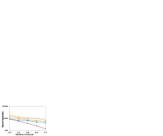
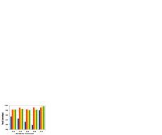
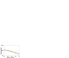
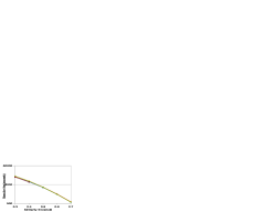
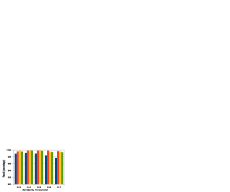
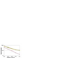
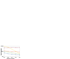
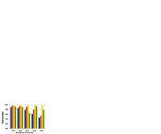
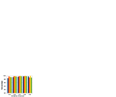
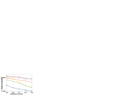
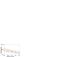
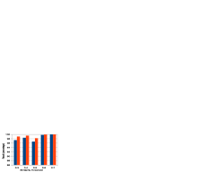
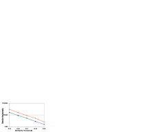
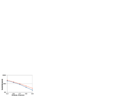
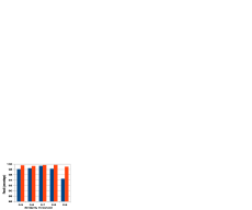
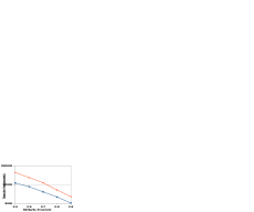
The performance and quality numbers are reported in Figure 2. We measure performance by the total execution time and we measure quality by recall (since we are giving probabilistic guarantees about recall). An added advantage of these methods is that since we compute exact similarity for all candidates that are retained and check whether they are above the threshold using exact similarity computation, all the strategies yield full precision (100%). Further more, the sequential hypothesis tests we do are truncated tests, i.e. we compute at most hashes, after which if a decision cannot be made, we send the pair for exact similarity computation. We report results on all the aforementioned datasets on both Jaccard and cosine similarity measures. For Jaccard, we vary the similarity threshold from and for cosine, we vary the threshold from . These are the same parametric settings used in the original BayesLSHLite work.
Results indicate that the pattern is quite similar for all the datasets. BayesLSHLite is always substantially faster in case of cosine similarity while in case of Jaccard similarity, AllPairs is marginally faster at times. At high values of the similarity threshold, SPRT is the slowest, while both One-Sided-CI-HT and Hybrid-HT performs very close to BayesLSHLite. This performance benefit comes from the one-sided tests. More precisely, choosing the width of the test based on the estimate first bin of hash comparisons makes each test optimized for the specific candidate being processed. Those tests are extremely efficient at pruning away false positive candidates whose true similarities are very far from the similarity threshold . The reason is these tests can allow a larger confidence width and hence less number of hash comparisons. Even the Hybrid-HT performs very well at such high thresholds, because it chooses one of the one-sided tests at such high threshold. However, at the other end of the spectrum, at very low similarity thresholds, the allowable confidence interval width becomes too small and a large number of trials is required by the one-sided tests making them inefficient. SPRT performs reasonably well under these situations. Under these conditions, the Hybrid-HT strategy is able to perform better than both (SPRT and One-Sided-CI-HT) as it able to smarty delegate pairs with true similarity close to threshold to SPRT instead of one-sided tests. In summary, the green lines (Hybrid-HT) can perform well through the whole similarity threshold range. For the WikiWords100K dataset in Figure 2(k) Hybrid-HT gave 8.8x speedup over AllPairs and 2.1x speedup of SPRT at 0.9 threshold and at 0.5 threshold, it gave 3.4x speedup over AllPairs and 1.3x speedup over SPRT.
In terms of quality, our proposed method One-Sided-CI-HT guarantee at least 97% recall (). In all results we see the recall of One-Sided-CI-HT, as expected, is above 97%. Inspite of the fact that SPRT does not have strong guarantees in case of composite hypothesis, we see that SPRT performs quite well in all datasets. Since Hybrid-HT uses the One-Sided-CI-HT and SPRT, its quality numbers are also extremely good. Only BayesLSHLite, which does not model the hash comparisons as a sequential process, falls marginally below the 97% mark at some places. In summary, our tests can provide rigorous quality guarantees, while significantly improving the performance by over traditional SPRT.






5.2.2 Algorithms using Early Pruning and Approximate Similarity Estimation
The previous section discussed the algorithms which can be used when the explicit representation of the original data is available. We now describe results on two algorithms for which only the hash signatures needs to be stored rather than the entire dataset. These algorithms use the LSH index generation followed by candidate pruning, followed by approximate similarity estimation. We compare the following two techniques:
BayesLSH: This uses the same pruning technique as BayesLSHLite along with the concentration inference for similarity estimation.
Hybrid-HT-Approx: This is our sequential variant. It uses Hybrid-HT’s pruning technique along with the sequential fixed-width confidence interval generation strategy as described in section 4.2. We set .
We use the same parametric settings as before. The additional parameters required here are the estimation error bound and the coverage probability for the confidence interval . We set and . Again we measure performance by execution time. Here we measure quality by both recall and estimation error as we provide probabilistic guarantees on both.
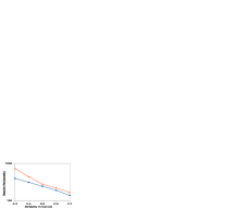
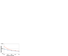
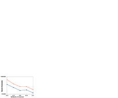
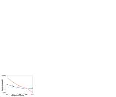
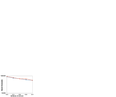
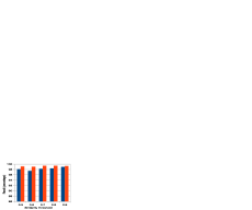
Figure 3 reports both the performance and recall numbers. We do not list the estimation error numbers as the avg. estimation error for each algorithm on each dataset was within the specified bound of 0.05. Results indicate that Hybrid-HT-Approx is slower than BayesLSH as expected, however is qualitatively better than BayesLSH. More importantly, in all cases, Hybrid-HT-Approx has a recall value which is well above the 97% guaranteed number. BayesLSH on an average performs quite well, however it does fall below the guaranteed recall value quite a few times. In summary, our method provides rigorous guarantees of quality without losing too much performance over BayesLSH.






6 Conclusions
In this paper we propose principled approaches of doing all pairs similarity search on a database of objects with a given similarity measure. We describe algorithms for handling two different scenarios - i) the original data set is available and the similarity of interest can be exactly computed from the explicit representation of the data points and ii) instead of the original dataset only a small sketch of the data is available and similarity needs to be approximately estimated. For both scenarios we use LSH sketches (specific to the similarity measure) of the data points. For the first case we develop a fully principled approach of adaptively comparing the hash sketches of a pair of points and do composite hypothesis testing where the hypotheses are similarity greater than or less than a threshold. Our key insight is a single test does not perform well for all similarity values, hence we dynamically choose a test for a candidate pair, based on a crude estimate of the similarity of the pair . For the second case we additionally develop an adaptive algorithm for estimating the approximate similarity between the pair. Our methods are based on finding sequential fixed-width confidence intervals. We compare our methods against state-of-the-art allpairs similarity search algorithms BayesLSH/Lite that does not precisely model the adaptive nature of the problem. We also compare against the more traditional sequential hypothesis testing technique – SPRT. We conclude that if quality guarantee is paramount, then we need to use our sequential confidence interval based techniques, and if performance is extremely important, then BayesLSH/Lite is the obvious choice. Our Hybrid models gives a very good tradeoff between the two extremes. We show that our hybrid method always guarantees the minimum-prescribed quality requirement (as specified by the input parameters), while being upto 2.1x faster than SPRT and 8.8x faster than AllPairs. Our hybrid method is also improves the recall by up to 5% over BayesLSH/Lite, a contemporary state-of-the-art adaptive LSH approach.
References
- [1] R. Bayardo, Y. Ma, and R. Srikant. Scaling up all pairs similarity search. In WWW, 2007.
- [2] A. Z. Broder, S. C. Glassman, M. S. Manasse, and G. Zweig. Syntactic clustering of the web. In WWW, 1997.
- [3] M. S. Charikar. Similarity estimation techniques from rounding algorithms. In STOC ’02, 2002.
- [4] M. Datar, N. Immorlica, P. Indyk, and V. Mirrokni. Locality-sensitive hashing scheme based on p-stable distributions. In SOCG, pages 253–262. ACM, 2004.
- [5] W. B. Frakes and R. Baeza-Yates. Information retrieval: data structures and algorithms. 1992.
- [6] J. Frey. Fixed-width sequential confidence intervals for a proportion. The American Statistician, 64(3), 2010.
- [7] A. Gionis, P. Indyk, and R. Motwani. Similarity search in high dimensions via hashing. In VLDB, 1999.
- [8] M. Girshick, F. Mosteller, and L. Savage. Unbiased estimates for certain binomial sampling problems with applications. In Selected Papers of Frederick Mosteller, pages 57–68. Springer, 2006.
- [9] M. Henzinger. Finding near-duplicate web pages: a large-scale evaluation of algorithms. In SIGIR, 2006.
- [10] P. Indyk and R. Motwani. Approximate nearest neighbors: towards removing the curse of dimensionality. In STOC, 1998.
- [11] B. Kulis and K. Grauman. Kernelized locality-sensitive hashing. Pattern Analysis and Machine Intelligence, IEEE Transactions on, 34(6):1092–1104, 2012.
- [12] H. Kwak, C. Lee, H. Park, and S. Moon. What is Twitter, a social network or a news media? In WWW, 2010.
- [13] D. Lewis, Y. Yang, T. Rose, and F. Li. Rcv1: A new benchmark collection for text categorization research. JMLR, 5:361–397, 2004.
- [14] D. Liben-Nowell and J. Kleinberg. The link-prediction problem for social networks. J. Am. Soc. Inf. Sci. Technol., 58:1019–1031, May 2007.
- [15] A. Mislove, M. Marcon, K. P. Gummadi, P. Druschel, and B. Bhattacharjee. Measurement and Analysis of Online Social Networks. In IMC, 2007.
- [16] D. Ravichandran, P. Pantel, and E. Hovy. Randomized algorithms and nlp: using locality sensitive hash function for high speed noun clustering. In ACL, 2005.
- [17] J. A. Rice. Mathematical statistics and data analysis. Cengage Learning, 2007.
- [18] V. Satuluri and S. Parthasarathy. Bayesian locality sensitive hashing for fast similarity search. Proceedings of the VLDB Endowment, 5(5):430–441, 2012.
- [19] A. Wald. Sequential analysis. Courier Corporation, 1973.
- [20] C. Xiao, W. Wang, X. Lin, and J. Yu. Efficient similarity joins for near duplicate detection. In WWW, 2008.
- [21] C. Xiao, W. Wang, X. Lin, J. X. Yu, and G. Wang. Efficient similarity joins for near duplicate detection. ACM Transactions on Database systems, 2011.
- [22] X. Zhu and A. Goldberg. Introduction to semi-supervised learning. Synthesis Lectures on Artificial Intelligence and Machine Learning, 3(1):1–130, 2009.