Analysis of Average Travel Time for Stateless Opportunistic Routing Techniques

Sateeshkrishna Dhuli, Department of Electrical Engineering,
Indian Institute of Technology,
Kanpur,
Email: dvsk@iitk.ac.in.
   Yatindra Nath Singh Department of Electrical Engineering,
Indian Institute of Technology,
Kanpur,
Email:ynsingh@iitk.ac.in.
Abstract

Wireless network applications, such as, searching, routing, self stabilization and query processing can be modeled as random walks on graphs. Stateless Opportunistic routing technique is a robust distributed routing technique based on random walk approach , where nodes transfer the packets to one of their direct neighbors uniformly, until the packets reach their destinations. Simplicity in execution, fault tolerance, low overhead and robustness to topology changes made it more suitable to wireless sensor networks scenarios. But the main disadvantage of stateless opportunistic routing is estimating and studying the effect of network parameters on the packet latency. In this work, we derived the analytical expressions for mean latency or average packet travel time for rπ‘Ÿr-nearest neighbor cycle, rπ‘Ÿr-nearest neighbor torus networks. Further, we derived the generalized expression for mean latency for mπ‘šm-dimensional rπ‘Ÿr-nearest neighbor torus networks and studied the effect of number of nodes, nearest neighbors and network dimension on average packet travel time.

Index Terms:
Wireless sensor networks, Delay tolerant networks, Random walks, Opportunistic forwarding, Spectral graph theory

I Introduction

In Stateless opportunistic routing, packets are forwarded to the next available neighbors in a random walk fashion until they reach the destinations. Estimation of access time, commute time, cover time and mixing time for random walks are discussed in [1]. Opportunistic forwarding provides significant performance gains and increases the throughput in the wireless networks [2], [3]. The problem of searching for a node or a piece of data and the hitting time of the node has been studied in [8]. Analytic formulas for maximum expected latency has been derived for regular wireless networks [7]. But this work does not studied the Mean Latency metric which is very important metric to study the packet delay and it also does not provide the upper and lower bounds for latency. In our work we derived the mean latency expressions for rπ‘Ÿr-nearest neighbor networks. The motivation behind the using finite sized networks is most of the practical WSN/adhoc networks are finite sized, such as applications in health, military and security in buildings. The rπ‘Ÿr-nearest neighbor networks [7] with varying number of nodes represents the notion of geographical proximity in the wireless sensor networks/ adhoc networks, where, nearest neighbors rπ‘Ÿr captures the overhead or nodes’ transmission radius. The advantage of this kind of analysis and theoretical results is they will play a critical role in the design of wireless sensor networks before the network operations, and also easier to perform than real experiments and thousands of simulation trails. This work provides the understanding of mean latency in terms of number of nodes, nearest neighbors and network dimension and gives the important insights for estimating latency in wireless networks. Further, we also studied the effect of wireless network parameters on packet delay in flat fading environments. For that, we used the system model proposed in [12] for designing the topology coefficients.

The rest of the paper is organized as follows. In Section II, we have given a brief overview about Mean Latency or average travel time. In Section III, we have given the generalized expressions for eigen values of the Laplacian matrix for rπ‘Ÿr-nearest neighbor networks. In Section IV, Mean Latency expressions and bounds are derived for rπ‘Ÿr-nearest neighbor cycle, rπ‘Ÿr-nearest neighbor torus and mπ‘šm-dimensional rπ‘Ÿr-nearest neighbor networks have been derived. In Section V, we have studied the network parameters effect on latency for arbitrary network model. In Section VI, we compared the simulation results with analytical results obtained in the Section IV.

II Mean Latency of Random Walks

Given an undirected graph G=(V,E)𝐺𝑉𝐸G=(V,E), where V𝑉V is the set of nodes and E𝐸E is the set of edges. Let A𝐴A be a adjacency matrix of G𝐺G and disubscript𝑑𝑖d_{i} be the degree of i𝑖i where each node i∈V𝑖𝑉i\in V. Let D=d​i​a​g​(di)π·π‘‘π‘–π‘Žπ‘”subscript𝑑𝑖D=diag\left({d_{i}}\right) be a diagonal matrix of node degrees, then P=Dβˆ’1​A𝑃superscript𝐷1𝐴P=D^{-1}A is a symmetric transition matrix associated with a random walk on G𝐺G. Let Ο€=[Ο€i]1≀i≀nπœ‹subscriptdelimited-[]subscriptπœ‹π‘–1𝑖𝑛\pi=\left[{\pi_{i}}\right]_{1\leq i\leq n} is a stationary distribution probability vector. In this case random walk on G𝐺G is reversible,.i.e. Ο€i​pi​j=Ο€j​pj​isubscriptπœ‹π‘–subscript𝑝𝑖𝑗subscriptπœ‹π‘—subscript𝑝𝑗𝑖\pi_{i}p_{ij}=\pi_{j}p_{ji} and distribution can be expressed as

Ο€i=diβˆ‘kdk=didsubscriptπœ‹π‘–subscript𝑑𝑖subscriptπ‘˜subscriptπ‘‘π‘˜subscript𝑑𝑖𝑑\pi_{i}=\frac{{d_{i}}}{{\sum\nolimits_{k}{d_{k}}}}=\frac{{d_{i}}}{d} (1)

Definition 1: Normalized Laplacian matrix for undirected graph G𝐺G is defined as

N=Dβˆ’12​(Dβˆ’A)​Dβˆ’12𝑁superscript𝐷12𝐷𝐴superscript𝐷12N=D^{-\frac{1}{2}}(D-A)D^{-\frac{1}{2}} (2)

Where N𝑁N is symmetric and positive semi-definite. Let Ξ»ksubscriptπœ†π‘˜\lambda_{k}, vksubscriptπ‘£π‘˜v_{k} be the eigen values and the corresponding eigen vectors of N𝑁N, then the hitting time of random walk [1] from node s𝑠s to node t𝑑t as Hs​tsubscript𝐻𝑠𝑑H_{st}, which can be expressed as

Hs​t=2​mβ€‹βˆ‘k=2n1Ξ»k​(vk​t2d​(t)βˆ’vk​s​vk​td​(t)​d​(s))subscript𝐻𝑠𝑑2π‘šsuperscriptsubscriptπ‘˜2𝑛1subscriptπœ†π‘˜superscriptsubscriptπ‘£π‘˜π‘‘2𝑑𝑑subscriptπ‘£π‘˜π‘ subscriptπ‘£π‘˜π‘‘π‘‘π‘‘π‘‘π‘ H_{st}=2m\sum\limits_{k=2}^{n}{\frac{1}{{\lambda_{k}}}}\left({\frac{{v_{kt}^{2}}}{{d(t)}}-\frac{{v_{ks}v_{kt}}}{{\sqrt{d(t)d(s)}}}}\right) (3)

L​e​m​m​aπΏπ‘’π‘šπ‘šπ‘ŽLemma 1: The mean latency or average random walk travel time T𝑇T [10] between every arbitrary pair of nodes is equal to

T=2nβˆ’1​T​r​(L+)𝑇2𝑛1π‘‡π‘Ÿsuperscript𝐿T=\frac{2}{{n-1}}Tr(L^{+}) (4)

Where T​r​(L+)π‘‡π‘Ÿsuperscript𝐿Tr(L^{+}) represents trace of the Moore-Penrose inverse of Laplacian matrix and n𝑛n denotes the number of nodes.

III rπ‘Ÿr-nearest neighbor networks

III-A rπ‘Ÿr-nearest neighbor cycle

The rπ‘Ÿr-nearest neighbor cycle CnrsuperscriptsubscriptπΆπ‘›π‘ŸC_{n}^{r} can be represented by a circulant matrix [4]. A circulant matrix is defined as

[a1a2……..anβˆ’1anan​a1​….….anβˆ’2​anβˆ’1........a3a4………..a1a2a2​a3​…​…​…​….an​a1]\left[\begin{array}[]{l}a_{1}\,\,a_{2}\,\,........a_{n-1}\,\,a_{n}\\ a_{n}\,\,a_{1}\,\,....\,....a_{n-2}\,a_{n-1}\\ .\,\,\,\,\,\,\,.\,\,\,\,\,\,\,\,\,\,\,\,\,\,\,\,\,\,\,\,\,\,\,\,.\,\,\,\,\,\,\,\,\,.\\ .\,\,\,\,\,\,\,.\,\,\,\,\,\,\,\,\,\,\,\,\,\,\,\,\,\,\,\,\,\,\,\,.\,\,\,\,\,\,\,\,\,.\\ a_{3}\,\,a_{4}\,\,\,...........a_{1}\,\,\,a_{2}\\ a_{2}\,\,a_{3}\,\,.............a_{n}\,\,a_{1}\\ \end{array}\right] (5)

and j𝑗j-th eigen value of a circulant matrix can be expressed as

Ξ»j=a1+a2Ο‰j+…………..+anΟ‰(nβˆ’1)​j\lambda_{j}=a_{1}+a_{2}\omega^{j}+..............+a_{n}\omega^{(n-1)j} (6)

where Ο‰πœ”\omega be the n𝑛n-th root of 1. Then Ο‰πœ”\omega is the complex number:

Ο‰=cos⁑(2​πn)+i​sin⁑(2​πn)=ei​2​πnπœ”2πœ‹π‘›π‘–2πœ‹π‘›superscript𝑒𝑖2πœ‹π‘›\omega=\cos\left({\frac{{2\pi}}{n}}\right)+i\sin\left({\frac{{2\pi}}{n}}\right)=e^{\frac{i2\pi}{n}} (7)

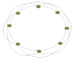
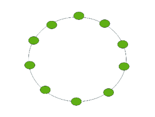
The 1-nearest cycle and 2-nearest cycle are shown in Fig.1 and Fig.2 respectively. Let the adjacency matrix A𝐴A and the degree matrix D𝐷D of 1-nearest cycle, then they can be written as

A=[0  1  0​…​…​…​…​..0  11  0  1​…​…​…​…​..0 0..........0  0  0​…​…​…​…​..0  11  0  0​…​…​…​…​..1 0]𝐴delimited-[]010…………..01101…………..00absentabsent000…………..01100…………..10A=\left[\begin{array}[]{l}0\,\,1\,\,0\,\,..............0\,\,1\\ 1\,\,0\,\,1\,\,..............0\,0\\ .\,\,\,\,.\,\,\,\,.\,\,\,\,\,\,\,\,\,\,\,\,\,\,\,\,\,\,\,\,\,\,\,\,\,.\,\,\,.\\ .\,\,\,\,.\,\,\,\,.\,\,\,\,\,\,\,\,\,\,\,\,\,\,\,\,\,\,\,\,\,\,\,\,\,.\,\,\,.\\ 0\,\,0\,\,0\,\,..............0\,\,1\\ 1\,\,0\,\,0\,\,..............1\,0\\ \end{array}\right] (8)
D=[2  0 0​…​…​…​…​0  00  2 0​….…​…​..0  0........0  0​…​…​…​…​…​2 00  0​…​…​…​…​…​0  2]𝐷delimited-[]200…………00formulae-sequence020………..00absentabsent00……………2000……………02D=\left[\begin{array}[]{l}2\,\,0\,0\,\,............0\,\,0\\ 0\,\,2\,0\,\,....\,........0\,\,0\\ .\,\,\,\,.\,\,\,\,\,\,\,\,\,\,\,\,\,\,\,\,\,\,\,\,\,\,\,\,\,\,\,\,\,.\,\,\,.\\ .\,\,\,\,.\,\,\,\,\,\,\,\,\,\,\,\,\,\,\,\,\,\,\,\,\,\,\,\,\,\,\,\,\,.\,\,\,.\\ 0\,\,0\,\,\,...............2\,0\\ 0\,\,0\,\,\,...............0\,\,2\\ \end{array}\right] (9)

T​h​e​o​r​e​mπ‘‡β„Žπ‘’π‘œπ‘Ÿπ‘’π‘šTheorem 1: The generalized expression for eigenvalues of Laplacian matrix L𝐿L for rπ‘Ÿr-nearest neighbor cycle CnrsuperscriptsubscriptπΆπ‘›π‘ŸC_{n}^{r} can be expressed as,

Ξ»j​(L​(Cnr))=2​r+1βˆ’sin⁑(2​r+1)​π​jnsin⁑π​jnsubscriptπœ†π‘—πΏsuperscriptsubscriptπΆπ‘›π‘Ÿ2π‘Ÿ12π‘Ÿ1πœ‹π‘—π‘›πœ‹π‘—π‘›\lambda_{j}(L(C_{n}^{r}))\,=2r+1-\frac{{\sin\frac{{(2r+1)\pi j}}{n}}}{{\sin\frac{{\pi j}}{n}}} (10)

where j=0,1,…​(nβˆ’1)𝑗01…𝑛1j=0,1,...(n-1).
P​r​o​o​fπ‘ƒπ‘Ÿπ‘œπ‘œπ‘“Proof: From (7), we can observe that, the first row is enough to obtain the eigen values of any circulant matrix.

The first row of adjacency matrix (A), degree matrix (D) and Laplacian matrix (L) can be written as follows,

A1​n=[0​ 1  1  1​…​…​..0​…​…​…​. 1  1  1⏟2​r​t​i​m​e​s]subscript𝐴1𝑛delimited-[]0subscript⏟111……..0……….1112π‘Ÿπ‘‘π‘–π‘šπ‘’π‘ A_{1n}=\left[{0\underbrace{\,1\,\,1\,\,1\,........0..........\,1\,\,1\,\,1}_{2r\,times}\,}\right] (11)
D1​n=[2​r​  0  0  0​…​..0  0  0  0]subscript𝐷1𝑛delimited-[]2π‘Ÿ000…..0000D_{1n}=\left[{2r\,\,0\,\,0\,\,0\,.....0\,\,0\,\,0\,\,0}\right] (12)

L1​n=[2​rβ€‹βˆ’1βˆ’1βˆ’1​…​..0​…​….βˆ’1βˆ’1βˆ’1⏟2​r​t​i​m​e​s]subscript𝐿1𝑛delimited-[]2π‘Ÿsubscript⏟formulae-sequence111…..0……1112π‘Ÿπ‘‘π‘–π‘šπ‘’π‘ L_{1n}=\left[{2r\,\,\underbrace{-1\,\,-1\,\,-1\,.....0...\,....-1\,-1\,-1}_{2r\,times}}\right]

(13)

By using (13) and (6), we can write the

Ξ»j​(L​(Cnr))=2​rβˆ’2β€‹βˆ‘i=1rcos⁑(2​π​j​in)subscriptπœ†π‘—πΏsuperscriptsubscriptπΆπ‘›π‘Ÿ2π‘Ÿ2superscriptsubscript𝑖1π‘Ÿ2πœ‹π‘—π‘–π‘›\lambda_{j}(L(C_{n}^{r}))=2r-2\sum\limits_{i=1}^{r}{\cos\left({\frac{{2\pi ji}}{n}}\right)} (14)

Lemma 2: Trigonometric identity of Dirichlet kernel [5]

1+2β€‹βˆ‘j=1rcos⁑(j​x)=sin⁑(r+12)​xsin⁑(x2)12superscriptsubscript𝑗1π‘Ÿπ‘—π‘₯π‘Ÿ12π‘₯π‘₯21+2\sum\limits_{j=1}^{r}{\cos(jx)}=\frac{{\sin\left({r+\frac{1}{2}}\right)x}}{{\sin\left({\frac{x}{2}}\right)}} (15)

Hence, from the Lemma 2, (14) can be rewritten as,
Ξ»j​(L​(Cnr))=2​r+1βˆ’sin⁑(2​r+1)​π​jnsin⁑π​jnsubscriptπœ†π‘—πΏsuperscriptsubscriptπΆπ‘›π‘Ÿ2π‘Ÿ12π‘Ÿ1πœ‹π‘—π‘›πœ‹π‘—π‘›\lambda_{j}(L(C_{n}^{r}))\,=2r+1-\frac{{\sin\frac{{(2r+1)\pi j}}{n}}}{{\sin\frac{{\pi j}}{n}}}
Refer to caption
Figure 1: 1-nearest neighbor cycle
Refer to caption
Figure 2: 2-nearest neighbor cycle

III-B rπ‘Ÿr-nearest neighbor torus

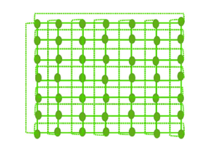
A torus can be seen in Fig. 3 and it can be represented by the nΓ—n𝑛𝑛n\times n block circulant matrix A𝐴A as

A=[A0A1……..An1βˆ’2An1βˆ’1An1βˆ’1​A0​….….An1βˆ’3​An1βˆ’2........A1A2​…​…​….An1βˆ’1​A0]A=\left[\begin{array}[]{l}A_{0}\,\,\,\,\,\,\,\,\,\,A_{1}\,\,........A_{n_{1}-2}\,\,A_{n_{1}-1}\\ A_{n_{1}-1}\,\,A_{0}\,\,....\,....A_{n_{1}-3}\,A_{n_{1}-2}\\ .\,\,\,\,\,\,\,\,\,\,\,\,\,\,\,\,\,\,\,\,\,.\,\,\,\,\,\,\,\,\,\,\,\,\,\,\,\,\,\,\,\,\,\,\,\,.\,\,\,\,\,\,\,\,\,\,\,\,\,\,\,.\\ .\,\,\,\,\,\,\,\,\,\,\,\,\,\,\,\,\,\,\,\,\,.\,\,\,\,\,\,\,\,\,\,\,\,\,\,\,\,\,\,\,\,\,\,\,\,.\,\,\,\,\,\,\,\,\,\,\,\,\,\,\,.\\ A_{1}\,\,\,\,\,\,\,\,\,\,\,\,\,A_{2}\,\,..........A_{n_{1}-1}\,\,A_{0}\\ \end{array}\right] (16)

where the number of nodes n=n12𝑛superscriptsubscript𝑛12n=n_{1}^{2}, then each block Aisubscript𝐴𝑖A_{i}, for i=0,1​…​(n1βˆ’1)𝑖01…subscript𝑛11i=0,1...(n_{1}-1) represents n1Γ—n1subscript𝑛1subscript𝑛1n_{1}\times n_{1} circulant matrices.

L​e​m​m​aπΏπ‘’π‘šπ‘šπ‘ŽLemma 2: Let G𝐺G be the cartesian product of two graphs Gβ€²superscript𝐺′G^{{}^{\prime}} and Gβ€²β€²superscript𝐺′′G^{{}^{\prime\prime}} with vertex sets Vβ€²superscript𝑉′V^{{}^{\prime}} and Vβ€²β€²superscript𝑉′′V^{{}^{\prime\prime}} and edge sets Eβ€²superscript𝐸′E^{{}^{\prime}} and Eβ€²β€²superscript𝐸′′E^{{}^{\prime\prime}}. Let the eigen values of Gβ€²superscript𝐺′G^{{}^{\prime}} are Ξ»1​(Gβ€²)​…​…​….Ξ»p​(Gβ€²)formulae-sequencesubscriptπœ†1superscript𝐺′………subscriptπœ†π‘superscript𝐺′\lambda_{1}\left({G^{{}^{\prime}}}\right)..........\lambda_{p}\left({G^{{}^{\prime}}}\right) and Gβ€²β€²superscript𝐺′′G^{{}^{\prime\prime}} are Ξ»1​(Gβ€²β€²)​…​…​….Ξ»q​(Gβ€²β€²)formulae-sequencesubscriptπœ†1superscript𝐺′′………subscriptπœ†π‘žsuperscript𝐺′′\lambda_{1}\left({G^{{}^{\prime\prime}}}\right)..........\lambda_{q}\left({G^{{}^{\prime\prime}}}\right), where p=|Vβ€²|𝑝superscript𝑉′p=\left|{V^{{}^{\prime}}}\right| and q=|Vβ€²β€²|π‘žsuperscript𝑉′′q=\left|{V^{{}^{\prime\prime}}}\right|. Let the vertex set of G𝐺G is r=|V|π‘Ÿπ‘‰r=\left|{V}\right|, which can be expressed as V=|Vβ€²|Γ—|Vβ€²β€²|𝑉superscript𝑉′superscript𝑉′′V=\left|{V^{{}^{\prime}}}\right|\times\left|{V^{{}^{\prime\prime}}}\right| [9]. Then, the eigen values of G𝐺G can be expressed as

Ξ»k​(G)=Ξ»i​(Gβ€²)+Ξ»j​(Gβ€²β€²)subscriptπœ†π‘˜πΊsubscriptπœ†π‘–superscript𝐺′subscriptπœ†π‘—superscript𝐺′′\lambda_{k}\left(G\right)=\lambda_{i}\left({G^{{}^{\prime}}}\right)+\lambda_{j}\left({G^{{}^{\prime\prime}}}\right) (17)

,where i∈{1,2,….p}i\in\{1,2,....p\}, j∈{1,2,….q}j\in\{1,2,....q\} and k∈{1,2,….r}k\in\{1,2,....r\}.

R​e​m​a​r​kπ‘…π‘’π‘šπ‘Žπ‘Ÿπ‘˜Remark 2: (17) also holds for eigen values of the Laplacians Lβ€²superscript𝐿′L^{{}^{\prime}} and Lβ€²β€²superscript𝐿′′L^{{}^{\prime\prime}} of graphs of Gβ€²superscript𝐺′G^{{}^{\prime}} and Gβ€²β€²superscript𝐺′′G^{{}^{\prime\prime}} respectively[6].

T​h​e​o​r​e​mπ‘‡β„Žπ‘’π‘œπ‘Ÿπ‘’π‘šTheorem 2: The generalized expression for eigenvalues of Laplacian matrix L𝐿L for rπ‘Ÿr-nearest neighbor torus Tnrsuperscriptsubscriptπ‘‡π‘›π‘ŸT_{n}^{r} can be expressed as

Ξ»j1,j2​(L​(Tk1,k2r))=4​r+2βˆ’sin⁑(2​r+1)​π​j1k1sin⁑π​j1k1βˆ’sin⁑(2​r+1)​π​j2k2sin⁑π​j2k2subscriptπœ†subscript𝑗1subscript𝑗2𝐿superscriptsubscript𝑇subscriptπ‘˜1subscriptπ‘˜2π‘Ÿ4π‘Ÿ22π‘Ÿ1πœ‹subscript𝑗1subscriptπ‘˜1πœ‹subscript𝑗1subscriptπ‘˜12π‘Ÿ1πœ‹subscript𝑗2subscriptπ‘˜2πœ‹subscript𝑗2subscriptπ‘˜2\lambda_{j_{1},j_{2}}\left({L(T_{k_{1},k_{2}}^{r})}\right)=4r+2-\frac{{\sin\frac{{(2r+1)\pi j_{1}}}{{k_{1}}}}}{{\sin\frac{{\pi j_{1}}}{{k_{1}}}}}-\frac{{\sin\frac{{(2r+1)\pi j_{2}}}{{k_{2}}}}}{{\sin\frac{{\pi j_{2}}}{{k_{2}}}}} (18)

where j1=0,1,2,…​(k1βˆ’1),j2=0,1,2,…​(k2βˆ’1)formulae-sequencesubscript𝑗1012…subscriptπ‘˜11subscript𝑗2012…subscriptπ‘˜21j_{1}=0,1,2,...(k_{1}-1),j_{2}=0,1,2,...(k_{2}-1).

P​r​o​o​fπ‘ƒπ‘Ÿπ‘œπ‘œπ‘“Proof : Tnrsuperscriptsubscriptπ‘‡π‘›π‘ŸT_{n}^{r} can be represented by Cartesian product of two rπ‘Ÿr-nearest neighbor cycles. So from the L​e​m​m​aπΏπ‘’π‘šπ‘šπ‘ŽLemma 2, we can write the Ξ»j1,j2​(L​(Tk1,k2r))subscriptπœ†subscript𝑗1subscript𝑗2𝐿superscriptsubscript𝑇subscriptπ‘˜1subscriptπ‘˜2π‘Ÿ\lambda_{j_{1},j_{2}}\left({L(T_{k_{1},k_{2}}^{r})}\right) as,

Ξ»j1,j2​(L​(Tk1,k2r))=Ξ»j1​(L​(Ck1r))+Ξ»j2​(L​(Ck2r))subscriptπœ†subscript𝑗1subscript𝑗2𝐿superscriptsubscript𝑇subscriptπ‘˜1subscriptπ‘˜2π‘Ÿsubscriptπœ†subscript𝑗1𝐿superscriptsubscript𝐢subscriptπ‘˜1π‘Ÿsubscriptπœ†subscript𝑗2𝐿superscriptsubscript𝐢subscriptπ‘˜2π‘Ÿ\lambda_{j_{1},j_{2}}\left({L(T_{k_{1},k_{2}}^{r})}\right)=\lambda_{j_{1}}\left({L(C_{k_{1}}^{r})}\right)+\lambda_{j_{2}}\left({L(C_{k_{2}}^{r})}\right) (19)

From R​e​m​a​r​kπ‘…π‘’π‘šπ‘Žπ‘Ÿπ‘˜Remark 2, we can write the expressions for Ξ»j1​(L​(Ck1r))subscriptπœ†subscript𝑗1𝐿superscriptsubscript𝐢subscriptπ‘˜1π‘Ÿ\lambda_{j_{1}}\left({L(C_{k_{1}}^{r})}\right) and Ξ»j2​(L​(Ck2r))subscriptπœ†subscript𝑗2𝐿superscriptsubscript𝐢subscriptπ‘˜2π‘Ÿ\lambda_{j_{2}}\left({L(C_{k_{2}}^{r})}\right), substituting them in (19) proves the theorem.

T​h​e​o​r​e​mπ‘‡β„Žπ‘’π‘œπ‘Ÿπ‘’π‘šTheorem 3: The generalized expression for eigenvalues of Laplacian matrix L𝐿L for mπ‘šm-dimensional rπ‘Ÿr-nearest neighbor torus can be expressed as

Ξ»j1,j2,…​jm​(L​(Tk1,k2​….kmr))=(2​r+1)​mβˆ’βˆ‘i=1m(sin⁑(2​r+1)​π​jikisin⁑π​jiki)subscriptπœ†subscript𝑗1subscript𝑗2…subscriptπ‘—π‘šπΏsuperscriptsubscript𝑇formulae-sequencesubscriptπ‘˜1subscriptπ‘˜2…subscriptπ‘˜π‘šπ‘Ÿ2π‘Ÿ1π‘šsuperscriptsubscript𝑖1π‘š2π‘Ÿ1πœ‹subscript𝑗𝑖subscriptπ‘˜π‘–πœ‹subscript𝑗𝑖subscriptπ‘˜π‘–\lambda_{j_{1},j_{2},...j_{m}}\left({L(T_{k_{1},k_{2}....k_{m}}^{r})}\right)=(2r+1)m-\sum\limits_{i=1}^{m}{\left({\frac{{\sin\frac{{(2r+1)\pi j_{i}}}{{k_{i}}}}}{{\sin\frac{{\pi j_{i}}}{{k_{i}}}}}}\right)}

(20)

P​r​o​o​fπ‘ƒπ‘Ÿπ‘œπ‘œπ‘“Proof: rπ‘Ÿr-nearest neighbor mπ‘šm-dimensional torus can be represented by Cartesian product of mπ‘šm number of rπ‘Ÿr-nearest neighbor cycles. So from the L​e​m​m​aπΏπ‘’π‘šπ‘šπ‘ŽLemma 2, we can write the Ξ»j1,j2​….jm​(L​(Tk1,k2​….kmr))subscriptπœ†formulae-sequencesubscript𝑗1subscript𝑗2…subscriptπ‘—π‘šπΏsuperscriptsubscript𝑇formulae-sequencesubscriptπ‘˜1subscriptπ‘˜2…subscriptπ‘˜π‘šπ‘Ÿ\lambda_{j_{1},j_{2}....j_{m}}\left({L(T_{k_{1},k_{2}....k_{m}}^{r})}\right) as,

Ξ»j1,j2,…​jm​(L​(Tk1,k2​….kmr))=Ξ»j1​(L​(Ck1r))+Ξ»j2​(L​(Ck1r))​…​…​…​….+Ξ»jm​(L​(Ckmr))formulae-sequencesubscriptπœ†subscript𝑗1subscript𝑗2…subscriptπ‘—π‘šπΏsuperscriptsubscript𝑇formulae-sequencesubscriptπ‘˜1subscriptπ‘˜2…subscriptπ‘˜π‘šπ‘Ÿsubscriptπœ†subscript𝑗1𝐿superscriptsubscript𝐢subscriptπ‘˜1π‘Ÿsubscriptπœ†subscript𝑗2𝐿superscriptsubscript𝐢subscriptπ‘˜1π‘Ÿβ€¦β€¦β€¦β€¦subscriptπœ†subscriptπ‘—π‘šπΏsuperscriptsubscript𝐢subscriptπ‘˜π‘šπ‘Ÿ\lambda_{j_{1},j_{2},...j_{m}}\left({L(T_{k_{1},k_{2}....k_{m}}^{r})}\right)=\lambda_{j_{1}}\left({L(C_{k_{1}}^{r})}\right)+\lambda_{j_{2}}\left({L(C_{k_{1}}^{r})}\right).............+\lambda_{j_{m}}\left({L(C_{k_{m}}^{r})}\right)

(21)

From R​e​m​a​r​kπ‘…π‘’π‘šπ‘Žπ‘Ÿπ‘˜Remark 2, we can substitute the expressions for Ξ»j1​(L​(Ck1r))subscriptπœ†subscript𝑗1𝐿superscriptsubscript𝐢subscriptπ‘˜1π‘Ÿ\lambda_{j_{1}}\left({L(C_{k_{1}}^{r})}\right), Ξ»j2​(L​(Ck2r))subscriptπœ†subscript𝑗2𝐿superscriptsubscript𝐢subscriptπ‘˜2π‘Ÿ\lambda_{j_{2}}\left({L(C_{k_{2}}^{r})}\right) and Ξ»jm​(L​(Ckmr))subscriptπœ†subscriptπ‘—π‘šπΏsuperscriptsubscript𝐢subscriptπ‘˜π‘šπ‘Ÿ\lambda_{j_{m}}\left({L(C_{k_{m}}^{r})}\right) in (21), which proves the theorem.

Refer to caption
Figure 3: Two dimensional torus

IV Mean latency analysis for rπ‘Ÿr-nearest neighbor networks

T​h​e​o​r​e​mπ‘‡β„Žπ‘’π‘œπ‘Ÿπ‘’π‘šTheorem 5: The mean latency T𝑇T of rπ‘Ÿr-nearest neighbor cycle CnrsuperscriptsubscriptπΆπ‘›π‘Ÿ{C_{n}^{r}} between every arbitrary pair of nodes is

T​(Cnr)=βˆ‘j=2n(2(nβˆ’1)​((2​r+1)βˆ’sin⁑(2​r+1)​π​jnsin⁑π​jn))𝑇superscriptsubscriptπΆπ‘›π‘Ÿsuperscriptsubscript𝑗2𝑛2𝑛12π‘Ÿ12π‘Ÿ1πœ‹π‘—π‘›πœ‹π‘—π‘›T\left({C_{n}^{r}}\right)=\sum\limits_{j=2}^{n}{\left({\frac{2}{{(n-1)\left({(2r+1)-\frac{{\sin\frac{{(2r+1)\pi j}}{n}}}{{\sin\frac{{\pi j}}{n}}}}\right)}}}\right)}

(22)

Proof: From (10), we can write

T​r​(L+)=βˆ‘j=2n1Ξ»j​(L)=βˆ‘j=2n(1((2​r+1)βˆ’sin⁑(2​r+1)​π​jnsin⁑π​jn))π‘‡π‘Ÿsuperscript𝐿superscriptsubscript𝑗2𝑛1subscriptπœ†π‘—πΏabsentsuperscriptsubscript𝑗2𝑛12π‘Ÿ12π‘Ÿ1πœ‹π‘—π‘›πœ‹π‘—π‘›\begin{array}[]{l}Tr(L^{+})=\sum\limits_{j=2}^{n}{\frac{1}{{\lambda_{j}(L)}}}\\ \,\,\,\,\,\,\,\,\,\,\,\,\,\,\,=\sum\limits_{j=2}^{n}{\left({\frac{1}{{\left({(2r+1)-\frac{{\sin\frac{{(2r+1)\pi j}}{n}}}{{\sin\frac{{\pi j}}{n}}}}\right)}}}\right)}\\ \end{array} (23)

Substituting the (23) in (4), proves the theorem.

T​h​e​o​r​e​mπ‘‡β„Žπ‘’π‘œπ‘Ÿπ‘’π‘šTheorem 6: The mean latency of rπ‘Ÿr-nearest neighbor torus Tk1,k2rsuperscriptsubscript𝑇subscriptπ‘˜1subscriptπ‘˜2π‘ŸT_{k_{1},k_{2}}^{r} between every arbitrary pair of nodes is

T​(Tk1,k2r)=βˆ‘j1=1k1βˆ’1βˆ‘j2=0k2βˆ’1(2(k1+k2βˆ’1)​((4​r+2)βˆ’sin⁑(2​r+1)​π​j1k1sin⁑π​j1k1βˆ’sin⁑(2​r+1)​π​j2k2sin⁑π​j2k2))𝑇superscriptsubscript𝑇subscriptπ‘˜1subscriptπ‘˜2π‘Ÿsuperscriptsubscriptsubscript𝑗11subscriptπ‘˜11superscriptsubscriptsubscript𝑗20subscriptπ‘˜212subscriptπ‘˜1subscriptπ‘˜214π‘Ÿ22π‘Ÿ1πœ‹subscript𝑗1subscriptπ‘˜1πœ‹subscript𝑗1subscriptπ‘˜12π‘Ÿ1πœ‹subscript𝑗2subscriptπ‘˜2πœ‹subscript𝑗2subscriptπ‘˜2T(T_{k_{1},k_{2}}^{r})=\sum\limits_{j_{1}=1}^{k_{1}-1}{\sum\limits_{j_{2}=0}^{k_{2}-1}{\left({\frac{2}{{\left({k_{1}+k_{2}-1}\right)\left({(4r+2)-\frac{{\sin\frac{{(2r+1)\pi j_{1}}}{{k_{1}}}}}{{\sin\frac{{\pi j_{1}}}{{k_{1}}}}}-\frac{{\sin\frac{{(2r+1)\pi j_{2}}}{{k_{2}}}}}{{\sin\frac{{\pi j_{2}}}{{k_{2}}}}}}\right)}}}\right)}}

(24)

Proof: From (18), we can write

T​r​(L+)=βˆ‘j1=1k1βˆ’1βˆ‘j2=0k2βˆ’11Ξ»j1,j2​(L)=βˆ‘j1=1k1βˆ’1βˆ‘j2=0k2βˆ’1(2((4​r+2)βˆ’sin⁑(2​r+1)​π​j1k1sin⁑π​j1k1βˆ’sin⁑(2​r+1)​π​j2k2sin⁑π​j2k2))π‘‡π‘Ÿsuperscript𝐿superscriptsubscriptsubscript𝑗11subscriptπ‘˜11superscriptsubscriptsubscript𝑗20subscriptπ‘˜211subscriptπœ†subscript𝑗1subscript𝑗2𝐿absentsuperscriptsubscriptsubscript𝑗11subscriptπ‘˜11superscriptsubscriptsubscript𝑗20subscriptπ‘˜2124π‘Ÿ22π‘Ÿ1πœ‹subscript𝑗1subscriptπ‘˜1πœ‹subscript𝑗1subscriptπ‘˜12π‘Ÿ1πœ‹subscript𝑗2subscriptπ‘˜2πœ‹subscript𝑗2subscriptπ‘˜2\begin{array}[]{l}Tr(L^{+})=\sum\limits_{j_{1}=1}^{k_{1}-1}{\sum\limits_{j_{2}=0}^{k_{2}-1}{\frac{1}{{\lambda_{j_{1},j_{2}}(L)}}}}\\ \,\,\,\,\,\,\,\,\,\,\,\,\,\,\,=\sum\limits_{j_{1}=1}^{k_{1}-1}{\sum\limits_{j_{2}=0}^{k_{2}-1}{\left({\frac{2}{{\left({(4r+2)-\frac{{\sin\frac{{(2r+1)\pi j_{1}}}{{k_{1}}}}}{{\sin\frac{{\pi j_{1}}}{{k_{1}}}}}-\frac{{\sin\frac{{(2r+1)\pi j_{2}}}{{k_{2}}}}}{{\sin\frac{{\pi j_{2}}}{{k_{2}}}}}}\right)}}}\right)}}\\ \end{array} (25)

Substituting the (25) in (4), proves the theorem.

T​h​e​o​r​e​mπ‘‡β„Žπ‘’π‘œπ‘Ÿπ‘’π‘šTheorem 7: The mean latency of rπ‘Ÿr-nearest neighbor torus Tk1,k2,….kmrsuperscriptsubscript𝑇formulae-sequencesubscriptπ‘˜1subscriptπ‘˜2…subscriptπ‘˜π‘šπ‘ŸT_{k_{1},k_{2},....k_{m}}^{r} between every arbitrary pair of nodes is

T​(Tk1,k2,….kmr)=βˆ‘j1=1k1βˆ’1βˆ‘j2=0k2βˆ’1β€¦β€‹β€¦β€‹βˆ‘jm=0kmβˆ’1(2((2​r+1)​mβˆ’βˆ‘i=1msin⁑(2​r+1)​π​jikisin⁑π​jiki))𝑇superscriptsubscript𝑇formulae-sequencesubscriptπ‘˜1subscriptπ‘˜2…subscriptπ‘˜π‘šπ‘Ÿsuperscriptsubscriptsubscript𝑗11subscriptπ‘˜11superscriptsubscriptsubscript𝑗20subscriptπ‘˜21……superscriptsubscriptsubscriptπ‘—π‘š0subscriptπ‘˜π‘š122π‘Ÿ1π‘šsuperscriptsubscript𝑖1π‘š2π‘Ÿ1πœ‹subscript𝑗𝑖subscriptπ‘˜π‘–πœ‹subscript𝑗𝑖subscriptπ‘˜π‘–T(T_{k_{1},k_{2},....k_{m}}^{r})=\sum\limits_{j_{1}=1}^{k_{1}-1}{\sum\limits_{j_{2}=0}^{k_{2}-1}{......\sum\limits_{j_{m}=0}^{k_{m}-1}{\left({\frac{2}{{\left({(2r+1)m-\sum\limits_{i=1}^{m}{\frac{{\sin\frac{{(2r+1)\pi j_{i}}}{{k_{i}}}}}{{\sin\frac{{\pi j_{i}}}{{k_{i}}}}}}}\right)}}}\right)}}}

(26)

Proof: From (20), we can write

T​r​(L+)=βˆ‘j1=1k1βˆ’1βˆ‘j2=0k2βˆ’1β€¦β€‹β€¦β€‹βˆ‘jm=0kmβˆ’11Ξ»j1,j2…..jm​(L)=βˆ‘j1=1k1βˆ’1βˆ‘j2=0k2βˆ’1β€¦β€‹β€¦β€‹βˆ‘jm=0kmβˆ’1(2(βˆ‘i=1mkiβˆ’1)​((2​r+1)​mβˆ’βˆ‘i=1msin⁑(2​r+1)​π​jikisin⁑π​jiki))\begin{array}[]{l}Tr(L^{+})=\sum\limits_{j_{1}=1}^{k_{1}-1}{\sum\limits_{j_{2}=0}^{k_{2}-1}{......\sum\limits_{j_{m}=0}^{k_{m}-1}{\frac{1}{{\lambda_{j_{1},j_{2}.....j_{m}}(L)}}}}}\\ \,\,\,\,\,\,\,\,\,\,\,\,\,\,\,=\sum\limits_{j_{1}=1}^{k_{1}-1}{\sum\limits_{j_{2}=0}^{k_{2}-1}{......\sum\limits_{j_{m}=0}^{k_{m}-1}{\left({\frac{2}{{\left({\sum\limits_{i=1}^{m}{k_{i}-1}}\right)\left({(2r+1)m-\sum\limits_{i=1}^{m}{\frac{{\sin\frac{{(2r+1)\pi j_{i}}}{{k_{i}}}}}{{\sin\frac{{\pi j_{i}}}{{k_{i}}}}}}}\right)}}}\right)}}}\\ \end{array}

(27)

Substituting the (27) in (4), proves the theorem.

L​e​m​m​aπΏπ‘’π‘šπ‘šπ‘ŽLemma 3: The mean latency T𝑇T between every arbitrary pair of nodes satisfies the following bound [11]:

2(nβˆ’1)​λ1​(L)≀T≀2Ξ»1​(L)2𝑛1subscriptπœ†1𝐿𝑇2subscriptπœ†1𝐿\frac{2}{{(n-1)\lambda_{1}(L)}}\leq T\leq\frac{2}{{\lambda_{1}(L)}} (28)

Where Ξ»1​(L)subscriptπœ†1𝐿\lambda_{1}(L) is the second smallest eigen value of Laplacian matrix and n𝑛n represents number of nodes.

T​h​e​o​r​e​mπ‘‡β„Žπ‘’π‘œπ‘Ÿπ‘’π‘šTheorem 8: The bounds for mean latency T𝑇T for rπ‘Ÿr-nearest neighbor cycle can be expressed as,

2​sin⁑πn(nβˆ’1)​((2​r+1)​sin⁑πnβˆ’sin⁑(2​r+1)​πn)≀T≀2​sin⁑πn(2​r+1)​sin⁑πnβˆ’sin⁑(2​r+1)​πn2πœ‹π‘›π‘›12π‘Ÿ1πœ‹π‘›2π‘Ÿ1πœ‹π‘›π‘‡2πœ‹π‘›2π‘Ÿ1πœ‹π‘›2π‘Ÿ1πœ‹π‘›\frac{{2\sin\frac{\pi}{n}}}{{(n-1)((2r+1)\sin\frac{\pi}{n}-\sin\frac{{(2r+1)\pi}}{n})}}\leq T\leq\frac{{2\sin\frac{\pi}{n}}}{{(2r+1)\sin\frac{\pi}{n}-\sin\frac{{(2r+1)\pi}}{n}}}

(29)

Proof: Substituting the n=1 in (4) gives Ξ»1​(L)subscriptπœ†1𝐿\lambda_{1}(L), which can be substituted in the (28) proves the theorem.

Similarly we can prove the bounds for mean latency for mπ‘šm-dimensional torus network as

2​sin⁑πk1(nβˆ’1)​((2​r+1)​sin⁑πk1βˆ’sin⁑(2​r+1)​πk1)≀T≀2​sin⁑πk1(2​r+1)​sin⁑πk1βˆ’sin⁑(2​r+1)​πk12πœ‹subscriptπ‘˜1𝑛12π‘Ÿ1πœ‹subscriptπ‘˜12π‘Ÿ1πœ‹subscriptπ‘˜1𝑇2πœ‹subscriptπ‘˜12π‘Ÿ1πœ‹subscriptπ‘˜12π‘Ÿ1πœ‹subscriptπ‘˜1\frac{{2\sin\frac{\pi}{{k_{1}}}}}{{(n-1)((2r+1)\sin\frac{\pi}{{k_{1}}}-\sin\frac{{(2r+1)\pi}}{{k_{1}}})}}\leq T\leq\frac{{2\sin\frac{\pi}{{k_{1}}}}}{{(2r+1)\sin\frac{\pi}{{k_{1}}}-\sin\frac{{(2r+1)\pi}}{{k_{1}}}}}

(30)

V Opportunistic Forwarding for arbitrary networks

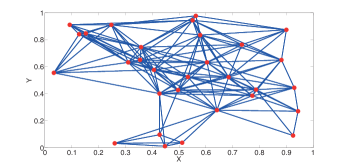
We consider the arbitrary network model as shown in Fig. 9, where the nodes are distributed arbitrarily, but their positions are known. The following propagation model has been considered

PRj=pi​j1+(ri​j​/​r0)Ξ·subscript𝑃subscript𝑅𝑗subscript𝑝𝑖𝑗1superscriptsubscriptπ‘Ÿπ‘–π‘—/subscriptπ‘Ÿ0πœ‚P_{R_{j}}=\frac{{p_{ij}}}{{1+\left({{{r_{ij}}\mathord{\left/{\vphantom{{r_{ij}}{r_{0}}}}\right.\kern-1.2pt}{r_{0}}}}\right)^{\eta}}} (31)

where PRjsubscript𝑃subscript𝑅𝑗P_{R_{j}} is the power received by node j𝑗j when node i𝑖i transmits, ri​jsubscriptπ‘Ÿπ‘–π‘—r_{ij} is the distance between nodes i𝑖i and j𝑗j, Ξ·πœ‚\eta is the path loss exponent and r0subscriptπ‘Ÿ0r_{0} is a reference distance. If ri​j≫r0much-greater-thansubscriptπ‘Ÿπ‘–π‘—subscriptπ‘Ÿ0r_{ij}\gg r_{0}, the receiver is in the transmit antenna far-field, where the received power is inversely proportional to ri​jΞ·superscriptsubscriptπ‘Ÿπ‘–π‘—πœ‚r_{ij}^{\eta}. Conversely, if ri​jβ‰ͺr0much-less-thansubscriptπ‘Ÿπ‘–π‘—subscriptπ‘Ÿ0r_{ij}\ll r_{0}, then the received power is approximately equal to the transmitted power.

The relationship between the coefficients ai​jsubscriptπ‘Žπ‘–π‘—a_{ij} and the distances ri​jsubscriptπ‘Ÿπ‘–π‘—r_{ij} can be expressed as

ai​j=11+(ri​j​/​rci​j)Ξ±subscriptπ‘Žπ‘–π‘—11superscriptsubscriptπ‘Ÿπ‘–π‘—/subscriptπ‘Ÿsubscript𝑐𝑖𝑗𝛼a_{ij}=\frac{1}{{1+\left({{{r_{ij}}\mathord{\left/{\vphantom{{r_{ij}}{r_{c_{ij}}}}}\right.\kern-1.2pt}{r_{c_{ij}}}}}\right)^{{}^{\alpha}}}} (32)

where α𝛼\alpha is a positive coefficient and rci​jsubscriptπ‘Ÿsubscript𝑐𝑖𝑗r_{c_{ij}} is the coverage radius, which depends on the transmit power.

From the (32), the relationship between the coverage radius rci​jsubscriptπ‘Ÿsubscript𝑐𝑖𝑗r_{c_{ij}}, power coefficients pi​jsubscript𝑝𝑖𝑗p_{ij} and the minimum required power for communication pm​i​nsubscriptπ‘π‘šπ‘–π‘›p_{min} can be expressed as

rci​j=r0​(pi​jpminβˆ’1)1​/​ηsubscriptπ‘Ÿsubscript𝑐𝑖𝑗subscriptπ‘Ÿ0superscriptsubscript𝑝𝑖𝑗subscript𝑝11/πœ‚r_{c_{ij}}=r_{0}\left({\frac{{p_{ij}}}{{p_{\min}}}-1}\right)^{{\raise 2.1097pt\hbox{$1$}\!\mathord{\left/{\vphantom{1\eta}}\right.\kern-1.2pt}\!\lower 2.1097pt\hbox{$\eta$}}} (33)

where

r0=l​o​g​(n)+cnπ​nsubscriptπ‘Ÿ0π‘™π‘œπ‘”π‘›subscriptπ‘π‘›πœ‹π‘›r_{0}=\sqrt{\frac{log(n)+c_{n}}{\pi n}} (34)

using the (33) and (31) the topology coefficients can be written in terms of the power coefficients pi​jsubscript𝑝𝑖𝑗p_{ij}, denoting the power used by node i𝑖i to transmit to node j𝑗j as

ai​j=r0α​(pi​jβˆ’pmin)α​/​ηr0α​(pi​jβˆ’pmin)α​/​η+ri​jα​pminα​/​ηsubscriptπ‘Žπ‘–π‘—superscriptsubscriptπ‘Ÿ0𝛼superscriptsubscript𝑝𝑖𝑗subscript𝑝𝛼/πœ‚superscriptsubscriptπ‘Ÿ0𝛼superscriptsubscript𝑝𝑖𝑗subscript𝑝𝛼/πœ‚superscriptsubscriptπ‘Ÿπ‘–π‘—π›Όsuperscriptsubscript𝑝𝛼/πœ‚a_{ij}=\frac{{r_{0}^{\alpha}\left({p_{ij}-p_{\min}}\right)^{{\raise 2.1097pt\hbox{$\alpha$}\!\mathord{\left/{\vphantom{\alpha\eta}}\right.\kern-1.2pt}\!\lower 2.1097pt\hbox{$\eta$}}}}}{{r_{0}^{\alpha}\left({p_{ij}-p_{\min}}\right)^{{\raise 2.1097pt\hbox{$\alpha$}\!\mathord{\left/{\vphantom{\alpha\eta}}\right.\kern-1.2pt}\!\lower 2.1097pt\hbox{$\eta$}}}+r_{ij}^{\alpha}p_{\min}^{{\raise 2.1097pt\hbox{$\alpha$}\!\mathord{\left/{\vphantom{\alpha\eta}}\right.\kern-1.2pt}\!\lower 2.1097pt\hbox{$\eta$}}}}} (35)

Remark 1 : From the (36), it is evident that the topology coefficients depends on power coefficients pi​jsubscript𝑝𝑖𝑗p_{ij} and other wireless network parameters α𝛼\alpha, pm​i​nsubscriptπ‘π‘šπ‘–π‘›p_{min}, r0subscriptπ‘Ÿ0r_{0}, ri​jsubscriptπ‘Ÿπ‘–π‘—r_{ij}, Ξ·πœ‚\eta.

Remark 2: From the (36) it is also evident that symmetric wireless links present in the network when pi​j=pj​isubscript𝑝𝑖𝑗subscript𝑝𝑗𝑖p_{ij}=p_{ji} and asymmetric wireless links exits when pi​jβ‰ pj​isubscript𝑝𝑖𝑗subscript𝑝𝑗𝑖p_{ij}\neq p_{ji}.
Here, we studied the symmetrical wireless networks.

VI Simulation results

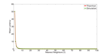
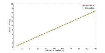
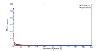
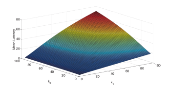
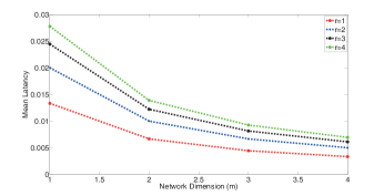
To validate the derived Mean latency analytical expressions, we compared with the simulation results and observed that both agree with each other. As shown in the Fig. 4, we plotted mean latency T𝑇T against nearest neighbors for n𝑛n=300, and observed that mean latency decreases with rπ‘Ÿr. From Fig.5, we can see the mean latency versus number of nodes n𝑛n for r=1π‘Ÿ1r=1 for rπ‘Ÿr-nearest neighbor cycle. Similarly to observe the Mean latency variation for two dimensional finite networks, we plotted mean latency versus k1subscriptπ‘˜1k_{1} and k2subscriptπ‘˜2k_{2}. We have taken rπ‘Ÿr=1 to plot Fig. 7. and k1subscriptπ‘˜1k_{1}=k2subscriptπ‘˜2k_{2}=1000 to plot Fig.6. To study the effect of network dimension on mean latency, we have taken the k1subscriptπ‘˜1k_{1}=16, k2subscriptπ‘˜2k_{2}=18, k3subscriptπ‘˜3k_{3}=20 and k4subscriptπ‘˜4k_{4}=22 and rπ‘Ÿr varied from 111 to 444. We have observed that, Mean latency is decreased with the network dimension and it further decreases with increase in rπ‘Ÿr.

To study the effect of few more wireless network parameters on expected packet delay (EPD), we have used the (3) and to generate the topologies as shown in Fig.9 we have used the (36).

E​P​D=βˆ‘i=1nβˆ‘j=1nHi​jn​(nβˆ’1)𝐸𝑃𝐷superscriptsubscript𝑖1𝑛superscriptsubscript𝑗1𝑛subscript𝐻𝑖𝑗𝑛𝑛1EPD=\frac{\sum_{i=1}^{n}\sum_{j=1}^{n}H_{ij}}{n(n-1)} (36)

where Hi​jsubscript𝐻𝑖𝑗H_{ij} denotes the delay between node i𝑖i and node j𝑗j and n𝑛n represents number of nodes.

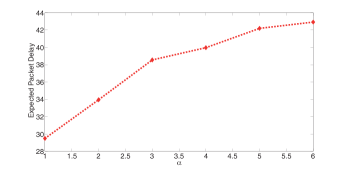
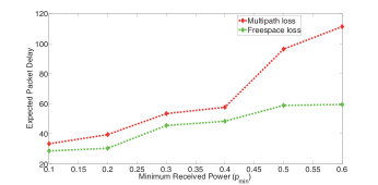
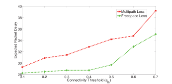
After estimating the EPD, we try to understand the effect of wireless network parameters on EPD.To evaluate how the network density affects the EPD, topologies has been generated with size, A=1Γ—1𝐴11A=1\times 1 m2superscriptπ‘š2m^{2}. From Fig. 10, we can see that, packet delay increases with path loss exponent, here we have taken pm​i​n=0.1subscriptπ‘π‘šπ‘–π‘›0.1p_{min}=0.1 and n=30𝑛30n=30. Fig. 11 shows the impact of Minimum Received Power on EPD for n=30𝑛30n=30 in freespace (Ξ±=2𝛼2\alpha=2) and multipath (Ξ±=4𝛼4\alpha=4) communication. From the simulation results, EPD increases with Minimum Received Power (pm​i​nsubscriptπ‘π‘šπ‘–π‘›p_{min}) and it increases further in multipath environments. From the proposed analytic modeling, topological coefficients has been derived and the connectivity threshold has been introduced to get the binary adjacency matrix which defines the wireless network topology. Fig. 12 shows the impact of connectivity threshold on EPD for pm​i​n=0.1subscriptπ‘π‘šπ‘–π‘›0.1p_{min}=0.1 in freespace (Ξ±=2𝛼2\alpha=2) and multipath (Ξ±=4𝛼4\alpha=4) communication.

Refer to caption
Figure 4: Mean latency versus Nearest neighbors for rπ‘Ÿr-nearest neighbor cycle
Refer to caption
Figure 5: Mean latency versus number of nodes for rπ‘Ÿr-nearest neighbor cycle
Refer to caption
Figure 6: Mean latency versus Nearest neighbors for rπ‘Ÿr-nearest neighbor torus
Refer to caption
Figure 7: Mean latency versus k1subscriptπ‘˜1k_{1} and k2subscriptπ‘˜2k_{2} for rπ‘Ÿr-nearest neighbor torus
Refer to caption
Figure 8: Mean latency versus Network Dimension for rπ‘Ÿr-nearest neighbor torus
Refer to caption
Figure 9: Wireless Network Topology
Refer to caption
Figure 10: Expected Packet Delay versus path loss exponent α𝛼\alpha
Refer to caption
Figure 11: Expected Packet Delay versus Pm​i​nsubscriptπ‘ƒπ‘šπ‘–π‘›P_{min} for random topology
Refer to caption
Figure 12: Expected Packet Delay versus Connectivity Threshold for random topology

VII Conclusions

In this work, analytical expressions for Mean latency or average travel time has been derived for rπ‘Ÿr-nearest neighbor cycle, rπ‘Ÿr-nearest neighbor torus and mπ‘šm dimensional rπ‘Ÿr nearest neighbor torus networks. We have given the theoretical bounds for mean latency in terms of number of nodes and nearest neighbors. Further, we also studied the latency for arbitrary wireless networks in flat fading environments.

References

  • [1] L.Β Lovasz, ”Random walks on graphs: A survey”, Combinatorics, Paul ErdΓΆs Is Eighty, vol. 2, pp. 1-46, 1993.
  • [2] S. Chachulski, M. Jennings, S. Katti, and D.Katabi, ”Trading structure for randomness in wireless opportunistic routing”, in Proc. ACM SIG- COMM, 2007, pp. 169-180.
  • [3] Biswas and R. Morris, ”ExOR: Opportunistic routing in multi-hop wireless networks”, in Proc. ACM SIGCOMM, 2005, pp. 133-144.
  • [4] D. Geller, I. Kra, S. Popescu, and S. Simanca, β€œOn circulant matrices,” http://www.math.sunysb.edu/∼sorin/, lecture notes.
  • [5] β€œWikipedia:Trigonometric identities,” http://en.wikipedia.org/wiki/ Trigonometric identity.
  • [6] R. Elsasser, B. Monien, R. Preis, A. Frommer, Optimal diffusion schemes and load balancing on product graphs, Parallel Processing Letters 14 (1) (2004) 61-73.
  • [7] C.-K. Chau and P. Basu, β€œAnalysis of latency of stateless opportunistic forwarding in intermittently connected networks,” IEEE/ACM Trans. Netw. , vol. 19, no. 4, pp. 1111-1124, Aug. 2011.
  • [8] C.-F. Hsin and M. Liu, ”Hitting time analysis for a class of random packet forwarding schemes in ad hoc networks”, Ad Hoc Netw., vol. 7, no. 3, pp. 500-515, May 2008.
  • [9] D.M.Cvetkovic, M.Doob, and H.Sachs. Spectra of graphs. Johann Anbrosius Barth, 3rd edition, 1995.
  • [10] A. Tizghadam and A. Leon-Garcia, β€œAutonomic Traffic Engineering for Network Robustness,” IEEE JSAC, vol. 28, no. 1, Jan. 2010, pp. 39-50.
  • [11] A. Tizghadam and A. Leon-Garcia. Survival Value of Communication Networks. Infocom Workshop on Network Science for Communications (NetSciCom), April 2009.
  • [12] S. Sardellitti, S. Barbarossa and A. Swami, ”Optimal Topology Control and Power Allocation for Minimum Energy Consumption in Consensus Networks,” IEEE Trans. on Signal Proc., Vol. 60, no. 1, pp. 383-399, January 2012.