Admittance of a long diffusive SNS junction

Abstract

The dynamical properties of hybrid normal metal/superconductor structures have recently come into research focus both experimentally and theoretically. Recent experimental studies of the coherent admittance $Y(\omega)$ of SNS rings as function of the phase difference $\phi_{0}$ are still not fully understood. Here we concentrate on the linear response regime, calculating $Y(\omega)$ by solving Usadel equations, linearised in electric field. Although partially reproducing previously known results, we find qualitatively different behaviour in the collisionless regime of $\tau_{in}^{-1}\ll\omega\lesssim E_{Th}$ and high temperature $T\gg E_{Th}$ and low temperature $T\lesssim E_{Th}$ near the minigap closing $\phi_{0}\sim\pi$. We find that the dissipative part $\mbox{Re}Y(\omega)$ peaks when the minigap closes (at a phase difference of $\pi$) even at high temperatures, when the equilibrium supercurrent is fully suppressed.

I Introduction

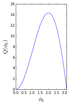
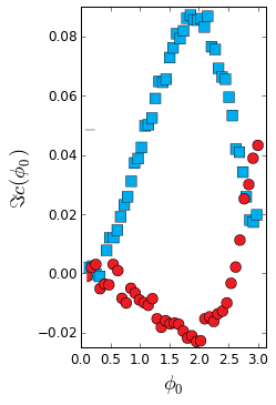
Figure 1: To the left: function $Q(\phi_{0})$, entering Lempitskii’s prediction for coherent part of the dissipation. To the right: Dissipative response ($c=\chi/\chi_{0}$) at $T\approx 17E_{Th}$, data from Ref. Dassonneville, 2014. Blue curve: hydrodynamic regime, $\hbar\omega=0.4E_{Th}$, red curve: collision-less regime, $\hbar\omega=2E_{Th}$ (arbitrary shifted in $c$ axis.)

The superconducting proximity effect on the transport properties of normal metal/superconductor structures has been thoroughly studied both theoretically and experimentally. Most of the studies were concentrated on properties of these systems in equilibriumPannetier and Courtois (2000). Recently, one of the most basic quantities, characterizing dynamical properties of such structures, - the admittance $Y\left(\omega\right)=I\left(\omega\right)/V\left(\omega\right)$, acquired more attention. It characterizes the current response $I\left(t\right)=\int\left(d\omega\right)I\left(\omega\right)e^{-i\omega t}$ to an ac voltage $V\left(t\right)=\int\left(d\omega\right)V\left(\omega\right)e^{-i\omega t}$ in the linear response regime.

The problem of calculation the current in the tunnelling (SIS) junction has been solved long ago for arbitrary time-dependent voltage $V(t)$Larkin and Ovchinnikov (1967). The phase dynamics of such a junction, coupled to the electromagnetic environment can usually be described by RSJC modelLikharev (1985). The same problem for a superconductor - normal metal - superconductor (SNS) junction is much more complicated, since the ac dynamics of the phase interferes here with the dynamics of the electrons in the normal metal. Additionally, multiple Andreev reflections are very important in such junctions, producing highly non-trivial energy distribution of the electrons in the wireZaitsev and Averin (1998); Bezuglyi et al. (2000); Cuevas et al. (2006), but they are not essential in the regime of small voltage which we concentrate on.

As follows, superconducting proximity effect causes $Y$ to be different from $Y_{N}=1/R_{N}$, the admittance of the wire in the normal state. Due to the Josephson relation $\dot{\phi}=2eV/\hbar$, the admittance can be related to the linear susceptibility of the junction with respect to the oscillating superconducting phase difference. In the geometry of an SNS ring, the phase difference $\phi$ $=-2\pi\frac{\Phi}{\Phi_{0}}$ (where $\Phi_{0}=h/2e$ is the flux quantum) is controlled by magnetic flux $\Phi$ penetrating this ring. The corresponding response function $\chi\left(\omega\right)=\frac{\delta I}{\delta\Phi}$ can be directly measured, and is related to $Y\left(\omega\right)$ as follows:

$$\chi\left(\omega\right)=i\omega Y\left(\omega\right).$$ (1)

In practice, the measurement of $\chi$ can be conducted by exposing the SNS ring to a weak magnetic field $B\left(t\right)=B_{0}+B_{osc}e^{-i\omega t}$. While $B_{0}$ fixes the stationary part of the superconducting phase difference along the normal wire $\phi_{0}=-2\pi\frac{\Phi}{\Phi_{0}}$, $B_{osc}$ generates an e.m.f. $\mathcal{E}\left(t\right)=-\frac{1}{c}\frac{d\Phi_{osc}}{dt}$, generating an $ac$ electric current.

In the static limit ($\omega\rightarrow 0$), $\mathcal{E}\left(t\right)$ is absent and the equilibrium response function $\chi\left(0\right)$ is recovered:

$$\chi\left(\omega=0\right)=-\frac{2\pi}{\Phi_{0}}\partial_{\phi}I_{S}\left(\phi_{0}\right),$$ (2)

where $I_{S}\left(\phi_{0}\right)$ stands for the current-phase relation of the junction in equilibrium. At finite frequency, the effect of $\mathcal{E}\left(t\right)$ is to both modify the non-dissipative response and to generate dissipation in the normal wire.

It can be expected that there should exist a limit, in which the admittance $Y$ of the junction equals the admittance of two $SN$ junctions connected in series. In this incoherent limit,  $Y$ is $\phi_{0}$-independent. As we will demonstrate shortly, it is achieved only when frequency is large $\omega\gg E_{Th}$, that is, the admittance has a significant coherent contribution even at very large temperature $T\gg E_{Th}$, but moderate frequency $\omega\lesssim E_{Th}$. This contribution will be the focus of our discussion. Another interesting point is that by measuring the response of the wire to $\mathcal{E}$ as a function of frequency and $dc$ phase difference $\phi_{0}$Chiodi et al. (2011); Dassonneville et al. (2013), one infers the dynamical properties of the Andreev levels in the junction through their effect on the conductive properties of the normal wire. This effect is thus very sensitive to inelastic processes in the wire and can be used as a specific probe.

From the theoretical side, the first study of the coherent contribution to the impedance of an SNS bridge was performed by LempitskiiLempitskii (1983). He considered the long junction limit ($E_{Th}\ll\Delta$) at high temperature ($T\gg E_{Th}$), biased in the adiabatic regime ($\hbar\omega\ll E_{Th}=\hbar D/L^{2}$), and obtained the following result:

$$Y\left(\omega\right)=Y_{N}\frac{E_{Th}}{T}\frac{E_{Th}/\hbar}{\tau_{in}^{-1}-i\omega}Q\left(\phi_{0}\right),$$ (3)

with $\tau_{in}$ staying for the inelastic relaxation time and universal function $Q\left(\phi_{0}\right)$ evaluated numerically. This function has recently been recalculated Virtanen et al. (2011) with better precision, see Fig. 1 for the result.

Lempitskii’s effect results from supercurrent-enhanced non-equilibrium population of Andreev levels in the wire. The most fascinating result is that this non-equilibrium population causes the coherent part of $Y$ to decay (at given $\tau_{in}$) slowly, as $E_{Th}/T,$ at $T\gg E_{Th}$, whereas the equilibrium supercurrent decays exponentially, as $\propto\exp\left(-L/L_{T}\right)$. This non-equilibrium enhancement of the superconducting correlations recalls the well known effect of the microwaves enhancement of superconductivity, the phenomena, known as the Dayem-Wyatt effectDayem and Wiegand (1967); Wyatt et al. (1966); Eliashberg (1970), which is observed in microbridges, thin films and stripesKommers and Clarke (1977); Dahlberg et al. (1979); Hall et al. (1980); Klapwijk et al. (1977); van den Hamer et al. (1984). Similar effect exist in the hybrid structuresNotarys et al. (1973); Warlaumont et al. (1979), but their physics is enriched by existence of two different time scales: time of diffusion along the normal part $\tau_{D}$ and inelastic scattering rate $\tau_{in}$, as was clearly demonstrated recently Chiodi et al. (2009). In our work, we concentrate on how this rich physics shows itself in the linear response function $Y$.

Since Lempitskii’s work, there was not much theoretical activity on the coherent contribution to $Y$ with notable exceptions provided byZhou and Spivak (1997); Argaman (1999). However, the recent experiments motivated a series of theoretical studies Virtanen et al. (2010, 2011); Ferrier et al. (2013). In particular, extensive numerical workVirtanen et al. (2010, 2011), supported by qualitative analytical treatment, was devoted to study $Y$ in a wide range of temperatures and frequencies.

Detailed comparison of the existent theoretical predictions to the experimental results was performed in Ref. Dassonneville, 2014. It was found that the non-dissipative response $\mbox{Im}Y$ of the junction can be well understood on the basis of Lempitskii’s theory for all moderate frequencies: $\hbar\omega\lesssim E_{Th}$ (In that experiment,$~{}E_{Th}=71mK$, corresponding to the frequency $f_{Th}=1.5GHz$). Interestingly, experimental results demonstrate that it is possible to follow the response function while it crosses over from hydrodynamic ($\omega\tau_{in}\ll 1$) to collision-less ($\omega\tau_{in}\gg 1$) regime, and extract inelastic scattering rate $\tau_{in}^{-1}$ as a function of temperature. At the highest temperature studied, $T\approx 1.2K$ it was found that $\tau_{in}\approx 2.5\tau_{D}$. Interestingly, the scattering rate, found in this experiment, demonstrates unusual temperature dependence, $\tau_{in}^{-1}\propto T^{2}$. We are not aware of any physical mechanism which can lead to such a dependence in a normal gold wire and believe that this power law is specific to the wire in the conditions of the proximity effect. We expect that it is related to the strong modification of the electronic spectrum in the wire by the superconducting contacts, which should influence electron-electron scattering processes - the effect which certainly deserves future studies.

Experimental results for hydrodynamic and collision-less regimes are presented by Fig. 1. In these figures, phase susceptibility is measured in natural units:

$$c=\chi/\chi_{0},$$ (4)

with $\chi_{0}=Y_{N}E_{Th}/\hbar$. Theoretical prediction for this quantity, obtained from Eqs (1) and (3), gives:

$$c^{th}=\frac{E_{Th}}{T}\frac{i\omega}{\tau_{in}^{-1}-i\omega}Q(\phi_{0}).$$ (5)

Fig. 1 illustrates one of the most important experimental observations: while at low frequency $\mbox{Im}c^{exp}$ fits well with Lempitskii’s result (see Fig. 1 for $Q\left(\phi_{0}\right)$), at higher frequency ($\omega\tau_{in}>1$) the dissipative response has a very different shape as a function of dc phase bias $\phi_{0}$. Recall that Eq. (5) results from the adiabatic calculation, which assumes $\omega\ll E_{Th}$. One may hope that the full numerical calculation (the one not relying on the expansion in $\omega/E_{Th}$) in this regime can describe the experimental results. Such a calculation, performed in the Ref. Virtanen et al., 2011 implies that the peak in $\mbox{Im}c^{exp}$ at minigap closing $\phi_{0}=\pi$ should be absent at $T\gg E_{Th}$, in clear contradiction with experiment.

This contradiction motivated a linear response analysis on the basis of BdG equations Ferrier et al. (2013). The results of the latter study seem to indicate qualitatively the presence of a maximum at $\phi_{0}=\pi$. From the theoretical side, it is clear that Lempitskii’s prediction concerns deviation from equilibrium of the Andreev pairs only, but quasi-particle excitations in the normal region can also be relevant, especially at not too low frequency. While it is clear that dissipation due to quasi-particles, excited by electric field, should be sharply peaked at $\phi_{0}=\pi$ at low temperatures $T\ll E_{Th}$, the fate of this peak at high temperature is not obvious a priori. As we mentioned above, it was predicted in Ref. Virtanen et al., 2011, that at high temperature this peak should disappear. Our goal is to reconsider this problem and to resolve the apparent contradiction between numerical results and experimental data in this regime.

We start with a simple observation: for the dissipative response the condition for validity of the adiabatic approximation is more stringent than for the non-dissipative one. Since the adiabatic contribution to $\mbox{Im}c$ decreases for $\omega\gtrsim\tau_{in}^{-1}$, the non-adiabatic (proportional to $\frac{\hbar\omega}{E_{Th}}$) correction to Eq (3) becomes essential already at $\hbar\omega\sim\sqrt{\hbar E_{Th}/\tau_{in}}\ll E_{Th}$. As we will show, the terms of the order of $\hbar\omega/E_{Th}$ result from the charge imbalance (induced by the ac electric field) and lead to the enhancement of dissipation at $\phi_{0}\approx\pm\pi$.

Our approach is based on the Usadel equation, expanded to the first order in the electric field, without assuming smallness of the proximity effect (in particular, we take into account all non-perturbative effects, such as the minigap). Although it is impossible to get a response function $Y\left(\omega,\phi_{0}\right)$ in closed form even in the simplest limiting cases, we go as far as possible analytically, resorting to numerical calculation only at the latest stage, which makes our calculation more controllable than fully numerical solution of the time-dependent Usadel equation.

II Usadel equation and linear response

II.1 General equations.

In what follows we make several additional simplifying assumptions: i) we treat the system as quasi one-dimensional, ii) we treat electron-electron interaction in the wire in the relaxation time approximation, neglecting possible energy and position dependence of the relaxation time as well as its modification by the proximity effect, and iii) we assume that $\Delta/E_{Th}\gg 1$. We measure the energy in units of $E_{Th}$ and length in units of $L$. Our starting point is Usadel equation ($e=-\left|e\right|$) in the presence of electric field. Due to gauge invariance, we are allowed to use scalar potential $\varphi$ instead of vector potential $\mathbf{A}$ to define an electric field in our quasi-one-dimensional normal wire: $E=-\nabla\varphi$. Then Usadel equation acquires the form:

$$\partial_{x}\left(\check{g}\cdot\partial_{x}\check{g}\right)+i\left[\epsilon\hat{\tau}^{3},\check{g}\right]+ie\left[\varphi,\hat{g}\right]=I_{St}\left[\check{g}\right].$$ (6)

In this equation $\check{g}\left(x,t,t^{\prime}\right)$ is isotropic part of quasi-classical Keldysh Green function, which is a matrix in the Nambu-Gorkov space. In terms of this function, the electric current can be expressed as follows ($S$ stands for the area’s wire):

$$I=\frac{\pi\sigma_{N}S}{4e}\mbox{tr}\left(\hat{\tau}^{3}\hat{\jmath}^{K}(t,t)\right),$$ (7)

where $\check{j}=\check{g}\cdot\nabla\check{g}.$

Neglecting spatial gradients in the superconducting reservoirs, we write for the Green function there:

$$\check{g}_{S}=\check{S}_{\phi}\cdot\check{g}_{eq}\cdot\check{S}_{\phi}^{+},$$ (8)

with

$$\check{S}\left(t,t^{\prime}\right)=\delta\left(t-t^{\prime}\right)e^{i\hat{\tau}_{3}e\int^{t}\varphi\left(\tau\right)d\tau}.$$ (9)

Here $\check{g}_{eq}$ is the equilibrium BCS Green function.

The Usadel equation (6) includes spectral and kinetic equations which may be obtained with the use of conventional parametrization $\hat{g}^{K}=\hat{g}^{R}\cdot\hat{H}-\hat{H}\cdot\hat{g}^{A}$, where $\hat{H}$ is a diagonal matrix of distribution functions in the Nambu-Gorkov space. In equilibrium, distribution function equals $\hat{H}=h\left(\epsilon\right)\hat{\tau}_{0},$ with $h\left(\epsilon\right)=\tanh\frac{\epsilon}{2T}.$ For retarded Green function the following parametrization is appropriate:

$$\hat{g}_{eq}^{R}\left(\epsilon,x\right)=\left(\begin{array}[]{cc}G&F\\ \bar{F}&-G\end{array}\right)$$ (10)

where $G=\cosh\theta,$ $F=\sinh\theta e^{i\phi},~{}\bar{F}=-\sinh\theta e^{-i\phi}$. In this parametrization, the spectral angle $\theta$ satisfies:

$$\partial_{x}^{2}\theta+\left(2i\epsilon-\tau_{in}^{-1}\right)\sinh\theta+J^{2}\frac{\cosh\theta}{\sinh^{3}\theta}=0,$$ (11)

where $J\equiv J(\epsilon)=i\sinh^{2}\theta\partial_{x}\phi$ is the spectral supercurrent, which is an integral of motion: $\partial_{x}J=0$ and we employed the relaxation time approximation. The boundary conditions for $\phi$ and $\theta$ are fixed by the BCS functions.

It is not feasible to write down the solutions of Eq (11) in a closed analytical form. However, the properties of the solutions are well known and numerical approaches to it are well developed. In order to obtain the solutions, we use publicly available solver, developed by P. Virtanen and T. Heikkila and described in Ref Virtanen and Heikkila, 2007. It provides Green function in the Ricatti parametrization, which is related to the trigonometric parametrization by means of the equations presented in the Appendix A.

Once the unperturbed solution is found, the effects of the weak electric field can be discussed. In the presence of oscillating electric potential $\varphi$, the Green function becomes time dependent: $\check{g}=\check{g}_{eq}+\delta\check{g}$. The effect of the electric field is twofold. First, it imposes time dependence on the phases of the order parameters in the superconducting contacts, see Eq. (8). This modifies the spectrum of the energy levels in the junction through corrections to retarded and advanced Green functions. Second, it induces inter-level transitions with energy transfer $\omega,$ changing the populations of these levels through corrections to the distribution function. Contributions of these two types of corrections to the electric current behave very differently at high temperatures: the former decay exponentially $\propto\exp\left(-L/L_{T}\right),$ while the latter decreases as a power-law with increasing the temperature.

II.2 Kinetic corrections.

Let us start with a discussion of the correction to the generalized distribution function $\delta\hat{H}$. It can be chosen diagonal in the particle-hole space:

$$\delta\hat{H}\left(\epsilon,\epsilon^{\prime},x\right)=\left[h_{L}\left(\epsilon,x\right)\hat{\tau}_{0}+h_{T}\left(\epsilon,x\right)\hat{\tau}_{3}\right]\delta\left(\epsilon-\epsilon^{\prime}-\omega\right)\text{.}$$

In the contacts, the transversal distribution function $h_{T}$ is driven out of equilibrium by the time-dependent voltage:

$$h_{T}\left(\epsilon,x=0,1\right)=h_{T,0}\left(\epsilon,x=0,1\right),$$ (12)

The function $h_{T}(\epsilon,x)$ describes charge imbalance that is induced in the N region due to oscillating electric field.

The longitudinal distribution function $h_{L}(\epsilon,x)$ describes all deviations from the equilibirum Fermi distribution function $h(\epsilon)$, which are related with non-equilibrium in energy distribution, but without any charge imbalance. $h_{L}(\epsilon,x)$ remains unperturbed within the linear response regime strictly at the boundaries with both superconductors:

$$h_{L}\left(\epsilon,x=0,1\right)=0,$$ (13)

however it varies sharply within a short distance near these boundaries, as will be discussed below.

In the wire, $h_{L,T}$ are governed by conservation laws of energy and charge currents:

$$\partial_{x}j_{L}+N\left(i\omega-\tau_{in}^{-1}\right)h_{L}=0,$$ (14)

$$\partial_{x}j_{T}+N\left(i\omega-\tau_{in}^{-1}\right)\left[h_{T}-h_{T0}\right]=0,$$ (15)

where relaxation time approximation is employed. Here

$$h_{T,0}\left(\epsilon,x\right)=e\varphi\left(x\right)\frac{h\left(\epsilon-\omega\right)-h\left(\epsilon\right)}{\omega},$$

and $h(\epsilon)=\tanh(\epsilon/2T)$ is equilibrium Fermi distribution function. Spatial distribution of the electric potential, $\varphi\left(x\right)$ has to be found from the Poisson equation:

$$\Delta\varphi=-\rho,$$ (16)

taking into account the fact that the oscillating voltage drop along the wire $Ve^{-i\omega t}=\varphi\left(0\right)-\varphi\left(1\right)$ is fixed by the applied ac phase modulation. In general, this gives a complicated coupled system of equations (6) and (16) which can be solved iteratively. In general, we find that for all frequencies of interest, the corrections to

$$\varphi\left(x\right)=\varphi\left(0\right)-Vxe^{-i\omega t},$$ (17)

which result from the charge redistribution in the wire do not lead to noticable modification of the coherent part of the admittance and we neglect them in what follows.

The energy current in Eq (14) reads:

$$j_{L}=D_{L}\partial_{x}h_{L}-\mathcal{T}\partial_{x}h_{T}+jh_{T},$$ (18)

and the charge current is equal to:

$$j_{T}=D_{T}\partial_{x}h_{T}+\mathcal{T}\partial_{x}h_{L}+jh_{L}.$$ (19)

The transport coefficients, which enter the definitions of the currents $j_{L,T},$ have the following physical meaning: $D_{L,T}$ are diffusion coefficients for energy and charge excitations, $\mathcal{T}$   is responsible for conversion of charge current to energy current and vice versa, while $N$ plays the role of the DOS of electron excitations. Finally, $j$ is determined by the spectral supercurrent $J$, see Eq.(38). These quantities are modified compared to their equilibrium values as a result of the time dependence of the electric field, see Appendix B for explicit expressions for them in terms of the unperturbed $\theta$ and $\phi$.

II.3 Spectral corrections.

Let us now turn to the corrections to the spectral functions, $\delta\hat{g}^{R\left(A\right)}$ (we will omit superscripts (R,A) below, since it can not lead to any confusion). Naively, each of these two matrices in the particle/hole space has four components:

$$\delta\hat{g}\left(\epsilon,\epsilon^{\prime},x\right)=\left(\begin{array}[]{cc}u_{pp}\left(\epsilon,x\right)&u_{ph}\left(\epsilon,x\right)\\ u_{hp}\left(\epsilon,x\right)&u_{hh}\left(\epsilon,x\right)\end{array}\right)\delta\left(\epsilon-\epsilon^{\prime}-\omega\right),$$ (20)

but the normalization condition $\delta\left(\hat{g}\cdot\hat{g}\right)=\hat{g}\cdot\delta\hat{g}+\delta\hat{g}\cdot\hat{g}=0$ allows to express diagonal components in terms of the off-diagonal ones:

$$\left(\begin{array}[]{c}u_{pp}\left(\epsilon\right)\\ u_{hh}\left(\epsilon\right)\end{array}\right)=\frac{\hat{M}}{1-\text{th}^{2}\frac{\theta}{2}\text{th}^{2}\frac{\theta_{-}}{2}}\left(\begin{array}[]{c}u_{ph}\left(\epsilon\right)\\ u_{hp}\left(\epsilon\right)\end{array}\right)$$ (21)

with matrix $M$ given by:

$$\hat{M}=\left(\begin{array}[]{cc}e^{i\phi_{-}}\text{th}\frac{\theta_{-}}{2}\left(1-\text{th}^{2}\frac{\theta}{2}\right)&-e^{i\phi}\text{th}\frac{\theta}{2}\left(1-\text{th}^{2}\frac{\theta_{-}}{2}\right)\\ -e^{-i\phi}\text{th}\frac{\theta}{2}\left(1-\text{th}^{2}\frac{\theta_{-}}{2}\right)&e^{i\phi_{-}}\text{th}\frac{\theta_{-}}{2}\left(1-\text{th}^{2}\frac{\theta}{2}\right)\end{array}\right)$$ (22)

and notation $f_{-}\left(\epsilon\right)=f\left(\epsilon-\omega\right)$ is used. Parametrization (21) reduces the number of independent components in $\delta\hat{g}$ to two: $u_{ph},~{}u_{hp}$. In the contacts, these functions are driven by the time-dependent voltage:

$$u_{ph}\left(\epsilon,x=0,1\right)=u_{ph,0}\left(\epsilon,x=0,1\right),$$ (23)

$$u_{ph,0}\left(\epsilon,x\right)=\frac{e^{i\phi}\sinh\theta+e^{i\phi_{-}}\sinh\theta_{-}}{\omega}e\varphi\left(x\right).$$ (24)

Similar equations valid for $u_{hp}$ can be obtained from Eqs.(23,24) by the replacement $\phi\rightarrow-\phi$. In the wire, functions $u_{ph}(x)$ and $~{}u_{hp}(x)$ are determined by the conservation laws of the spectral currents, which take the following form:

$$\partial_{x}j_{ph}+\left(2i\epsilon-i\omega-\tau_{in}^{-1}\right)u_{ph}+$$ (25)

$$+ie\varphi\left[e^{i\phi}\sinh\theta-e^{i\phi_{-}}\sinh\theta_{-}\right]=0.$$ (26)

Similar equation is valid for $u_{hp}$ and $j_{hp}$ with substitution $\phi\rightarrow-\phi$. The spectral currents read:

$$\left(\begin{array}[]{c}j_{ph}\\ j_{hp}\end{array}\right)=\hat{D}_{S}\left(\begin{array}[]{c}\partial_{x}u_{ph}\\ \partial_{x}u_{hp}\end{array}\right)+\hat{J}_{S}\left(\begin{array}[]{c}u_{ph}\\ u_{hp}\end{array}\right)\text{,}$$ (27)

where

$$\hat{D}_{S}=\left(\begin{array}[]{cc}D_{S}&e^{i\left(\phi+\phi_{-}\right)}\bar{D}_{S}\\ e^{-i\left(\phi+\phi_{-}\right)}\bar{D}_{S}&D_{S}\end{array}\right)$$ (28)

and

$$\hat{J}_{S}=\left(\begin{array}[]{cc}J_{S}+\frac{J+J_{-}}{\cosh\theta+\cosh\theta_{-}}&e^{i\left(\phi+\phi_{-}\right)}\bar{J}_{S}\\ e^{-i\left(\phi+\phi_{-}\right)}\bar{J}_{S}&J_{S}-\frac{J+J_{-}}{\cosh\theta+\cosh\theta_{-}}\end{array}\right).$$ (29)

The spectral transport coefficients $D_{S},\bar{D}_{S}$ and $J_{S},\bar{J}_{S}$ which enter these expressions, are provided in the Appendix B.

III Results

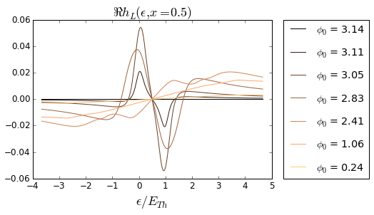
Figure 2: Variation of the longitudinal distribution function at $T=15E_{Th}$, $\hbar\omega=E_{Th}$ with varying the phase difference (color online).

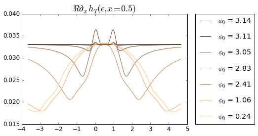
Figure 3: Variation of the transversal distribution function at $T=15E_{Th}$, $\hbar\omega=E_{Th}$ with varying the phase difference (color online).

We start our presentation from the exemplary results for the distribution functions, which are shown on the Figs 2, 3. In all the figures, for inelastic rate we have assumed $\hbar\tau_{in}^{-1}=T/g$ for definiteness (value of $g$ is given in the Figure captions).

Below, we discuss the results for the admittance $Y/Y_{N}$. For comparison with experiment, keep in mind, that dimensionless susceptibility to the oscillating phase, introduced in Eq. (4), reads $\chi/\chi_{0}=i\frac{\hbar\omega}{E_{Th}}Y/Y_{N}$. For the SNS junction of the experiment, mentioned in the introduction, $\chi_{0}\approx 35\mu A/\Phi_{0}$.

III.1 High temperature.

Let us discuss the variation of the dissipative part of the admittance with frequency at high temperature, see Figs. 4, 5. As expected, at low frequency, Lempitskii’s result is reproduced, see the curve corresponding to $\omega=0.1E_{Th}$. With growth of the frequency, the shape of the curve drastically changes and the dissipative part of $Y$ acquires a peak at $\phi_{0}=\pi,$ which becomes more prominent with growth of frequency and can be clearly seen up to the largest temperature of $T=15E_{Th}$.

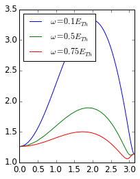
Figure 4: Variation of $\mbox{Re}Y(\phi_{0})/Y_{N}$ with frequency at $T=15E_{Th}$, $g=40$, low frequencies (color online).

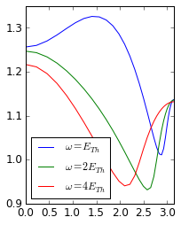
Figure 5: Variation of $\mbox{Re}Y(\phi_{0})/Y_{N}$ with frequency at $T=15E_{Th}$, $g=40$, high frequencies (color online).

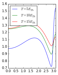
Figure 6: Variation of $\mbox{Re}Y(\phi_{0})/Y_{N}$ with temperature at $\hbar\omega=E_{Th}$, $g=40$ (color online).

The same kind of evolution of $\mbox{Re}Y(\phi_{0})/Y_{N}$ is shown for different temperatures at fixed frequency $\hbar\omega=E_{Th}$ in Fig.6. Note strong peak near phase equal to $\pi$ at $T=5E_{Th}$.

In order to understand this result, recall how Eq. (3) was derived. First, we note that at $T\gg E_{Th}$ the contribution of the spectral corrections $\delta\hat{g}$ to the electric current can be neglected and only corrections to the distribution function ($h_{L,T}$) are important. At finite voltage, the charge excitations, described by $h_{T},$ which enter the wire from the superconductor and get converted into energy excitations there, see the last term in Eq. (18). In the limit of $\hbar\omega/\Delta\ll 1$ the energy excitations (described by $h_{L}(\epsilon,x)$) are locked in between the superconducting contacts, since the corresponding density of states vanishes at the superconductors. Because of that, relatively large and almost spatially independent non-equilibrium correction to the longitudinal distribution function $h_{L}^{\left(\text{Lemp.}\right)}(\epsilon)=h_{L}(\epsilon)-h(\epsilon)$ in the wire is established:

$$h_{L}^{\left(\text{Lemp.}\right)}\approx\frac{j}{\left\langle N\right\rangle}\frac{eV}{i\omega+\tau_{in}^{-1}}h^{\prime}\left(\epsilon\right)\text{,}$$ (30)

which contributes to electric current as $I\propto\int jh_{L}^{\left(\text{Lemp.}\right)}d\epsilon$, leading to Eq. (3). Note that this equation seems to be inconsistent with the boundary condition, Eq. (13). In fact, in the limit $E_{Th}\ll\Delta$ true distribution function differs from $h_{L}^{\left(\text{Lemp.}\right)}$ in the closest vicinity of the boundary, where it exibits large spatial gradient and sharply varies from $h_{L}=0$ in the superconductor to $h_{L}=h_{L}^{\left(\text{Lemp.}\right)}$ in the wire. As a consequence, the limit of $\Delta\rightarrow\infty$ is singular: $h_{L}$ has a jump at $x=0$. Expanding the KE in the vicinity of the contact $x=0$ we find that Eq. (13) is replaced by an effective boundary condition:

$$\left.\partial_{x}h_{L}\left(\epsilon\right)\right|_{x=0}=\frac{\omega}{\zeta\left(\epsilon\right)}\left.h_{L}\left(\epsilon\right)\right|_{x=0},$$ (31)

where $\zeta\left(\epsilon\right)=$ $\left.\partial_{x}\theta_{-}^{A}\right|_{x=0}-\left.\partial_{x}\theta^{R}\right|_{x=0}$.

It is important that at low frequency $h_{L}$ is limited only by inelastic processes: in the limit of $\tau_{in}\rightarrow\infty$ one has $h_{L}\propto\frac{V}{T}\frac{E_{Th}}{\hbar\omega}$. This is why at lowest frequencies the correction to $h_{L}(\epsilon)$ leads to the whole effect dominated by the Lempitskii’s contribution. The properties of the transversal distribution function $h_{T}$ are quite different. It describes charge excitations which are free to leave the wire via Andreev reflection, so that corrections to $h_{T}$ are relatively small at the lowest frequencies: $h_{T}(\epsilon)\propto\frac{V}{T}$. However, it is clear that at $\hbar\omega\sim E_{Th}$ charged excitations described by $h_{T}(\epsilon)$ can provide an important contribution to electric current, comparable to that due to excitations of Andreev pairs (described by $h_{L}(\epsilon)$). If one is interested in dissipative part of $Y,$ the corresponding condition is even more stringent, since the real part of $h_{L}$ starts to decay already at $\hbar\omega\sim\hbar\tau_{in}^{-1}\ll E_{Th}$.

III.2 Low temperature.

At low temperature, the dissipation is noticeable only in the vicinity of the minigap closing, see Fig. 7. These results are very natural. Indeed, at $T=0$ dissipation is non-vanishing only as long as frequency is large enough compared to the minigap $E_{g}$, in particular, at $\omega=0$ one has $\mbox{Re}Y\propto\delta\left(\phi_{0}-\pi\right)$. This peak becomes broadens at finite temperature: $\delta\phi\propto\hbar\omega,T$. In addition, at finite $\omega$ it acquires additional structure: observe a kink of the dissipation as $\phi_{0}$ departures from $\pi$. The position of this kink is determined by the condition $2E_{g}\left(\phi_{k}\right)=\omega$. Indeed, for $\phi_{k}\sim\pi,$ one hasIvanov et al. (2002): $E_{g}\left(\phi\right)\approx\frac{\pi^{3}}{4}E_{Th}\left|1-\phi_{\phi}/\pi\right|$, which gives for $\hbar\omega=0.5E_{Th}$: $\phi_{k}\approx 3.04$. It can also be followed how this kink shifts with growth of the frequency. At larger temperature it becomes smoothened away, see for example the evolution of the curve on the Fig. (8) from $T=2E_{Th}$ to $T=5E_{Th}$.

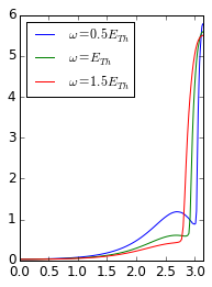
Figure 7: Variation of $\mbox{Re}Y(\phi_{0})/Y_{N}$ with frequency at $T=E_{Th}$, $g=40$ (color online).

III.3 Low frequency.

Another interesting crossover in the shape of $\mbox{Re}Y(\phi_{0})/Y_{N}$ is seen at low frequencies upon variation of the temperature. It is illustrated on the Fig. 8. At moderately low temperature $T=2E_{Th}$ strong peak of dissipation is found at the phase difference $\phi_{0}\approx 0.75\pi$; with temperature increase, this peak becomes more rounded and shifts further away from $\pi$, so that curve becomes more and more similar to Lempitskii’s function $Q_{0}\left(\phi\right)$.

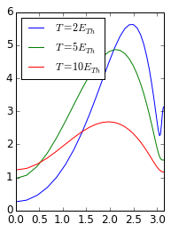
Figure 8: Variation of $\mbox{Re}Y(\phi_{0})/Y_{N}$ with temperature at $\omega=0.3E_{Th}$, $g=20$ (color online).

IV Conclusions

We have developed a fully microscopic approach to the calculation of a non-stationary ac linear response function of a S-N-S junction under the dc phase bias, that is valid at arbitrary relations between temperature $T$, Thouless energy $E_{Th}$ and frequency $\omega$. We assumed energy gap in the S terminals $\Delta$ to be much larger than all these energy scales and took into account inelastic relaxation rate $\hbar/\tau_{in}\leq E_{Th}$. The shape of the dissipative response $\mbox{Re}Y(\phi_{0})/Y_{N}$ is shown to be very sensitive to the relations between $T$, $E_{Th}$, $\hbar\omega$ and $\hbar/\tau_{in}$. Explicit results for the function $\mbox{Re}Y(\phi_{0})/Y_{N}$ can be found for any choice of the above parameters using the published codes. In particular, we have shown that accurate solution reproduces many of the qualitative features of the experimental resultsDassonneville (2014), including peak at the phase difference equal to $\pi$ at high frequencies and high temperature; we interpret this peak as the result of charge imbalance induced by high-frequency electric field. Still some quantitative disagreement exists: the experimental value of dissipation at $\phi_{0}=\pi$ is higher (at the same values of $T$ and $\omega$) than our computations provide. Possible source of this disagreement may be related with non-zero resistance of S-N interfaces which we did not took into account in the present calculations, since we assume interfaces to be perfectly transmitting. It is a straightforward task to include non-zero interface resistance into the calculational scheme developed.

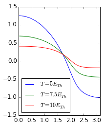
Figure 9: Variation of $\mbox{Im}Y(\phi_{0})/Y_{N}$ with temperature at $\omega=5E_{Th}$, $g=20$ (color online).

In our discussion, we did not touch the issue of the non-dissipative part of $Y\left(\phi_{0}\right),$ which, at moderate frequency, seems to be reasonably well described in the Lempitskii’s approximation. What lies outside this approximation is an interesting feature at high frequency at $\phi_{0}\sim\pi,$ which is observed in the experimentDassonneville (2014), as Fig. 6.21 of this reference shows. In our model, we obtain the flattening  of $\mbox{Im}Y$ at $\phi_{0}\sim\pi$ at $\omega\gtrsim E_{Th}$. For example, see Fig. 9 for the results at $\omega=5E_{Th}$, which at high temperature are rather close to the experiment. However, we do not see qualitative change of behaviour with lowering the temperature and do not get the large drop at $\phi_{0}=\pi$ which is observed in experiment. The nature of this drop is a very interesting problem for the future study. Another interesting problem is to include more realistic description of electron-electron interaction into the linear response calculation. It can be as interesting as important due to the specific spectral properties of the electrons, confined between superconducting reservoirs and great sensitivity of the admittance to inelastic processes in the experimentally relevant regime of frequency and temperature.

Acknowledgements. The authors gratefully acknowledge H. Bouchiat, B. Dassonneville, S. Gueron for careful reading of the manuscript and useful discussions and P. Virtanen for comments. KT thanks the members of the Institut für Theorie der Kondensierten Materie at KIT, where this work was started, for their kind hospitality. KT was supported by the Paul and Tina Gardner fund for Weizmann-TAMU collaboration and RFBR grant 13-02-00963.

Appendix A Ricatti parametrization of the GF

For numerical solution of unperturbed Usadel equation, it is more convenient to use Ricatti parametrization:

$$\hat{G}_{0}^{R}=\frac{1}{1-ab}\left(\begin{array}[c]{cc}1+ab&2a\\ -2b&-1-ab\end{array}\right).$$ (32)

In this parametrization, spectral Usadel equation reads:

$$Da^{\prime\prime}+2i\epsilon a=-\frac{2Dba^{\prime 2}}{1-ab},~{}Db^{\prime\prime}+2i\epsilon b=-\frac{2Dab^{\prime 2}}{1-ab}.$$ (33)

In the main part, we hold to trigonometric parametrization, see Eq (10), which makes formulae more compact. The relationship between the two parametrizations is as follows:

$$a=e^{i\phi}\text{th}\frac{\theta}{2},~{}b=e^{-i\phi}\text{th}\frac{\theta}{2}.$$ (34)

Appendix B Transport coefficients at finite frequency

Here we present expressions for transport coefficients at non-zero frequency, which enter Eqs (14), (15). Energy/charge diffusion coefficients read:

$$D_{L,T}=1-\cosh\theta^{R}\cosh\theta_{-}^{A}\pm\cos\left(\phi_{-}^{A}-\phi^{R}\right)\sinh\theta^{R}\sinh\theta_{-}^{A},$$ (35)

anomalous transport coefficient:

$$\mathcal{T}=-i\sin\left(\phi_{-}^{A}-\phi^{R}\right)\sinh\theta^{R}\sinh\theta_{-}^{A},$$ (36)

and density of states:

$$N=\cosh\theta^{R}-\cosh\theta_{-}^{A}.$$ (37)

Finally, the spectral supercurrent reads:

$$j=J^{R}-J_{-}^{A}$$ (38)

The frequency of oscillations enters these expression by the energy shifts, which are shown by the following notation: $f_{\pm}\left(\epsilon\right)=f\left(\epsilon\pm\omega\right)$. The spectral transport coefficients, which enter Eq (25) read:

$$D_{S}=\frac{1+\cosh\theta\cosh\theta_{-}}{\cosh\theta+\cosh\theta_{-}},$$ (39)

$$~{}\bar{D}_{S}=\frac{\sinh\theta\sinh\theta_{-}}{\cosh\theta+\cosh\theta_{-}}$$ (40)

and

$$J_{S}=\left(1+\cosh\theta\cosh\theta_{-}\right)\partial_{x}\frac{1}{\cosh\theta+\cosh\theta_{-}},$$ (41)

$$~{}\bar{J}_{S}=\sinh\theta\sinh\theta_{-}\partial_{x}\frac{1}{\cosh\theta+\cosh\theta_{-}}\text{.}$$ (42)

References

- Dassonneville (2014) B. Dassonneville, Ph.D. thesis (2014).
- Pannetier and Courtois (2000) B. Pannetier and H. Courtois, Journal of Low Temperature Physics 118, 5 (2000).
- Larkin and Ovchinnikov (1967) A. Larkin and Y. N. Ovchinnikov, Sov. Phys. JETP 24, 1035 (1967).
- Likharev (1985) K. Likharev, Moscow Izdatel Nauka 1 (1985).
- Zaitsev and Averin (1998) A. Zaitsev and D. Averin, Physical review letters 80, 3602 (1998).
- Bezuglyi et al. (2000) E. Bezuglyi, V. Shumeiko, G. Wendin, H. Takayanagi, et al., Physical Review B 62, 14439 (2000).
- Cuevas et al. (2006) J. Cuevas, J. Hammer, J. Kopu, J. Viljas, and M. Eschrig, Physical Review B 73, 184505 (2006).
- Chiodi et al. (2011) F. Chiodi, M. Ferrier, K. Tikhonov, P. Virtanen, T. Heikkilä, M. Feigelman, S. Guéron, and H. Bouchiat, Scientific Reports 1 (2011).
- Dassonneville et al. (2013) B. Dassonneville, M. Ferrier, S. Guéron, and H. Bouchiat, Physical Review Letters 110, 217001 (2013).
- Lempitskii (1983) S. Lempitskii, Sov. Phys. JETP 58 (1983).
- Virtanen et al. (2011) P. Virtanen, F. S. Bergeret, J. C. Cuevas, and T. T. Heikkilä, Physical Review B 83, 144514 (2011).
- Dayem and Wiegand (1967) A. H. Dayem and J. J. Wiegand, Phys. Rev. 155, 419 (1967), URL http://link.aps.org/doi/10.1103/PhysRev.155.419.
- Wyatt et al. (1966) A. F. G. Wyatt, V. M. Dmitriev, W. S. Moore, and F. W. Sheard, Phys. Rev. Lett. 16, 1166 (1966), URL http://link.aps.org/doi/10.1103/PhysRevLett.16.1166.
- Eliashberg (1970) G. Eliashberg, JETP Letters 11, 114 (1970).
- Kommers and Clarke (1977) T. Kommers and J. Clarke, Phys. Rev. Lett. 38, 1091 (1977), URL http://link.aps.org/doi/10.1103/PhysRevLett.38.1091.
- Dahlberg et al. (1979) E. Dahlberg, R. Orbach, and I. Schuller, Journal of Low Temperature Physics 36, 367 (1979), ISSN 0022-2291, URL http://dx.doi.org/10.1007/BF00118713.
- Hall et al. (1980) J. T. Hall, L. B. Holdeman, and R. J. Soulen, Phys. Rev. Lett. 45, 1011 (1980), URL http://link.aps.org/doi/10.1103/PhysRevLett.45.1011.
- Klapwijk et al. (1977) T. Klapwijk, J. van den Bergh, and J. Mooij, Journal of Low Temperature Physics 26, 385 (1977), ISSN 0022-2291, URL http://dx.doi.org/10.1007/BF00655418.
- van den Hamer et al. (1984) P. van den Hamer, T. Klapwijk, and J. Mooij, Journal of Low Temperature Physics 54, 607 (1984), ISSN 0022-2291, URL http://dx.doi.org/10.1007/BF00683622.
- Notarys et al. (1973) H. A. Notarys, M. L. Yu, and J. E. Mercereau, Phys. Rev. Lett. 30, 743 (1973), URL http://link.aps.org/doi/10.1103/PhysRevLett.30.743.
- Warlaumont et al. (1979) J. M. Warlaumont, J. C. Brown, T. Foxe, and R. A. Buhrman, Phys. Rev. Lett. 43, 169 (1979), URL http://link.aps.org/doi/10.1103/PhysRevLett.43.169.
- Chiodi et al. (2009) F. Chiodi, M. Aprili, and B. Reulet, Phys. Rev. Lett. 103, 177002 (2009), URL http://link.aps.org/doi/10.1103/PhysRevLett.103.177002.
- Zhou and Spivak (1997) F. Zhou and B. Spivak, JETP Letters 65, 369 (1997).
- Argaman (1999) N. Argaman, Superlattices and microstructures 25, 861 (1999).
- Virtanen et al. (2010) P. Virtanen, T. T. Heikkilä, F. S. Bergeret, and J. C. Cuevas, Physical Review Letters 104, 247003 (2010).
- Ferrier et al. (2013) M. Ferrier, B. Dassonneville, S. Gueron, and H. Bouchiat, Physical Review B 88, 174505 (2013).
- Virtanen and Heikkila (2007) P. Virtanen and T. Heikkila, Appl. Phys. A 89, 625 (2007), source code available at http://ltl.tkk.fi/ theory/usadel1/.
- Ivanov et al. (2002) D. A. Ivanov, R. von Roten, and G. Blatter, Physical Review B 66, 052507 (2002).