Bayesian $T$-optimal discriminating designs

Abstract

The problem of constructing Bayesian optimal discriminating designs for a class of regression models with respect to the $T$-optimality criterion introduced by Atkinson and Fedorov, 1975a is considered. It is demonstrated that the discretization of the integral with respect to the prior distribution leads to locally $T$-optimal discriminating design problems with a large number of model comparisons. Current methodology for the numerical construction of discrimination designs can only deal with a few comparisons, but the discretization of the Bayesian prior easily yields to discrimination design problems for more than $100$ competing models. A new efficient method is developed to deal with problems of this type. It combines some features of the classical exchange type algorithm with the gradient methods. Convergence is proved and it is demonstrated that the new method can find Bayesian optimal discriminating designs in situations where all currently available procedures fail.

Keyword and Phrases: Design of experiment, Bayesian optimal design; model discrimination; gradient methods; model uncertainty

AMS Subject Classification: 62K05

1 Introduction

Optimal design theory provides useful tools to improve the accuracy of statistical inference without any additional costs by carefully planning experiments before they are conducted. Numerous authors have worked on the construction of optimal designs in various situations. For many models optimal designs have been developed explicitly [see the monographs of Pukelsheim, (2006); Atkinson et al., (2007)] and several algorithms have been developed for their numerical construction if the optimal designs are not available in explicit form [see Yu, (2010); Yang et al., (2013) among others]. On the other hand the construction of such designs depends sensitively on the model assumptions and an optimal design for a particular model might be inefficient if it is used in a different model. Moreover, in many experiments it is often not obvious which model should be finally fitted to the data and model building is an important part of data analysis. A typical and very important example are Phase II dose-finding studies, where various nonlinear regression models of the form

(1.1) $$Y=\eta(x,\theta)+\varepsilon.$$

have been developed for describing the dose-response relation [see Pinheiro et al., (2006)], but the problem of model uncertainty arises in nearly any other statistical application. As a consequence, the construction of efficient designs for model identification has become an important field in optimal design theory. Early work can be found in Stigler, (1971), who determined designs for discriminating between two nested univariate polynomials by minimizing the volume of the confidence ellipsoid for the parameters corresponding to the extension of the smaller model. Several authors have worked on this approach in various other classes of nested models [see for example Dette and Haller, (1998) or Song and Wong, (1999) among others].
A different approach to the problem of constructing optimal designs for model discrimination is given in a pioneering paper by Atkinson and Fedorov, 1975a , who proposed the $T$-optimality criterion to construct designs for discriminating between two competing regression models. Roughly speaking their approach provides a design such that the sum of squares for a lack of fit test is large. Atkinson and Fedorov, 1975b extended this method for discriminating a selected model $\eta_{1}$ from a class of other regression models, say $\{\eta_{2},\ldots,\eta_{k}\}$, $k\geq 2$. In contrast to the work Stigler, (1971) and followers the $T$-optimality criterion does not require competing nested models and has found considerable attention in the statistical literature with numerous applications including such important fields as chemistry or pharmacokinetics [see e.g. Atkinson et al., (1998), Ucinski and Bogacka, (2005), López-Fidalgo et al., (2007), Atkinson, (2008), Tommasi, (2009) or Foo and Duffull, (2011) for some more recent references]. A drawback of the $T$-optimality criterion consists of the fact that – even in the case of linear models – the criterion depends on the parameters of the model $\eta_{1}$. This means that $T$-optimality is a local optimality criterion in the sense of Chernoff, (1953), and that it requires some preliminary knowledge regarding the parameters. Consequently, most of the cited papers refer to locally $T$-optimal designs. Although there exist applications where such information is available [for example in the analysis of dose response studies as considered in Pinheiro et al., (2006)], in most situations such knowledge can be rarely provided. Several authors have introduced robust versions of the classical optimality criteria such as Bayesian or minimax $D$-optimality criteria in order to determine efficient designs for model discrimination, which are less sensitive with respect to the choice of parameters [see Pronzato and Walter, (1985); Chaloner and Verdinelli, (1995); Dette, (1997)]. The robustness problem of the $T$-optimality criterion has been already mentioned in Atkinson and Fedorov, 1975a , who proposed a Bayesian approach to address the problem of parameter uncertainty in the $T$-optimality criterion. Wiens, (2009) imposed (linear) neighbourhoud structures on each regression response and determined least favorable points in these neighbourhouds in order to robustify the locally $T$-optimal design problem. Dette et al., (2012) considered polynomial regression models and determined explicitly Bayesian $T$-optimal discriminating designs for the criterion introduced by Atkinson and Fedorov, 1975a . Their results indicate the difficulties arising in Bayesian $T$-optimal design problems.
The scarcity of literature on Bayesian $T$-optimal discriminating designs can be explained by the fact that in nearly all cases of practical interest these designs have to be found numerically, and even this is a very hard problem. These numerical difficulties become even apparent in the case of locally $T$-optimal designs. Atkinson and Fedorov, 1975a proposed an exchange type algorithm, which has a rather slow rate of convergence and has been used by several authors. Braess and Dette, (2013) pointed out that, besides its slow convergence, this algorithm does not yield the solution of the optimal discriminating design problem, if more than $5$ model comparisons are under consideration. These authors developed a more efficient algorithm for the determination of locally $T$-optimal discriminating designs for several competing regression models by exploring relations between optimal design problems and (nonlinear) vector-valued approximation theory. Although the resulting algorithm provides a substantial improvement of the exchange type methods it cannot deal with Bayesian optimality criteria in general, and the development of an efficient procedure for this purpose is a very challenging and open problem.
The goal of the present paper is to fill this gap. We utilize the fact that in applications the integral with respect to the prior distribution has to be determined by a discrete approximation and we show that the discrete Bayesian $T$-optimal design problem is a special case of the local $T$-optimality criterion for a very large number of competing models considered as in Braess and Dette, (2013). The competing models arise from the different support points used for the approximation of the prior distribution by a discrete measure, and the number of model comparisons in the resulting criterion easily exceeds the $200$. Therefore the algorithm in Braess and Dette, (2013) does not provide a solution of the corresponding optimization problem, and we propose a new method for the numerical construction of Bayesian $T$-optimal designs with substantial computational advantages. Roughly speaking, the support points of the design in each iteration are determined in a similar manner as proposed in Atkinson and Fedorov, 1975a but for the calculation of the corresponding weights we use a gradient approach. It turns out that the new procedure is extremely efficient and is able to find Bayesian $T$-optimal designs with a few number of iterations.
The remaining part of this paper is organized as follows. In Section 2 we give an introduction into the problem of designing experiments for discriminating between competing regression models and also derive some basic properties of locally $T$-optimal discriminating designs. In particular we show how the Bayesian $T$-optimal design problem is related to a local one with a large number of model comparisons [see Section 2.2]. Section 3 is devoted to the construction of new numerical procedures (in particular Algorithm 3.2), for which we prove convergence to a $T$-optimal discriminating design. Our approach consists of two steps consecutively optimizing with respect to the support points (Step 1) and weights of the design (Step 2). For the second step we also discuss two procedures to speed up the convergence of the algorithm. The results are illustrated in Section 4 calculating several Bayesian $T$-optimal discriminating designs in examples, where all other available procedure do not provide a numerical solution of the optimal design problem. For example, the new procedure is able to solve locally $T$-optimal designs with more than $240$ model comparisons as they are arising frequently in Bayesian $T$-optimal design problems. In particular we illustrate the methodology calculating Bayesian $T$-optimal discriminating designs for a dose finding clinical trial which has recently been discussed in Pinheiro et al., (2006). The corresponding R-package will be provided in the CRAN library. Finally all proof are deferred to an appendix in Section 5.

2 $T$-optimal discriminating designs

Consider the regression model (1.1), where $x$ belongs to some compact set $\mathcal{X}$ and observations at different experimental conditions are independent. For the sake of transparency and a clear representation we assume that the error $\varepsilon$ is normally distributed. The methodology developed in the following discussion can be extended to more general error structures following the line of research in López-Fidalgo et al., (2007), but details are omitted for the sake of brevity.

Throughout this paper we consider the situation where $\nu$ different models, say

(2.1) $$\eta_{i}(x,\theta_{i}),\qquad i=1,\dots,\nu,$$

are available to describe the dependency of $Y$ on the predictor $x$. In (2.1) the quantity $\theta_{i}$ denotes a $d_{i}$-dimensional parameter, which varies in a compact space, say $\Theta_{i}$ ($i=1,\ldots,\nu$). Following Kiefer, (1974) we consider approximate designs that are defined as probability measures, say $\xi$, with finite support. The support points $x_{1},\ldots,x_{k}$ of a design $\xi$ give the locations where observations are taken, while the weights $\omega_{1},\ldots,\omega_{k}$ describe the relative proportions of observations at these points. If an approximate design is given and $n$ observations can be taken, a rounding procedure is applied to obtain integers $n_{i}$ ($i=1,\ldots,k)$ from the not necessarily integer valued quantities $\omega_{i}n$ such that $\sum_{i=1}^{k}n_{i}=n$. We are interested in designing an experiment, such that a most appropriate model can be chosen from the given class $\{\eta_{1},\ldots,\eta_{\nu}\}$ of competing models.

2.1 $T$-optimal designs

In the case of $\nu=2$ competing models Atkinson and Fedorov, 1975a proposed to fix one model, say $\eta_{1}(\cdot,\theta_{1})$, with corresponding parameter $\overline{\theta}_{1}$ and to maximize the functional

(2.2) $$T_{12}(\xi)=\inf_{\theta_{2}\in\Theta_{2}}\int_{\mathcal{X}}\Big{[}\eta_{1}(x,\overline{\theta}_{1})-\eta_{2}(x,\theta_{2})\Big{]}^{2}\xi(dx),$$

in the class of all (approximate) designs. Roughly speaking, these designs maximize the power of the test of the hypothesis ”$\eta_{1}$ versus $\eta_{2}$” . Note that the resulting optimal design depends on the parameter $\overline{\theta}_{1}$ for the first model, which has to be fixed by the experimenter. This means that these designs are local in the sense of Chernoff, (1953). It was pointed out by Dette et al., (2013) that locally $T$-optimal designs may be very sensitive with respect to misspecification of $\overline{\theta}_{1}$. In a further paper Atkinson and Fedorov, 1975b generalized their approach to construct optimal discriminating designs for more than $2$ competing regression models and suggested the criterion

(2.3) $$T(\xi)=\min_{2\leq j\leq\nu}T_{1j}(\xi)=\min_{2\leq j\leq\nu}\inf_{\theta_{j}\in\Theta_{j}}\int_{\mathcal{X}}\Big{[}\eta_{1}(x,\overline{\theta}_{1})-\eta_{j}(x,\theta_{j})\Big{]}^{2}\xi(dx).$$

This criterion determines a ”good” design for discriminating the model $\eta_{1}$ against $\eta_{2},\ldots,\eta_{\nu}$, where the parameter $\overline{\theta}_{1}$ has the same meaning as before. As pointed out by Tommasi and López-Fidalgo, (2010) and Braess and Dette, (2013) there are many situations, where it is not clear which model should be considered as fixed and these authors proposed a symmetrized Bayesian (instead of minimax) version of the $T$-optimality criterion, that is

(2.4) $$T_{\mathrm{P}}(\xi)=\sum_{i,j=1}^{\nu}p_{i,j}T_{i,j}(\xi)=\sum_{i,j=1}^{\nu}p_{i,j}\inf_{\theta_{i,j}\in\Theta_{j}}\int_{\mathcal{X}}\Big{[}\eta_{i}(x,\overline{\theta}_{i})-\eta_{j}(x,\theta_{i,j})\Big{]}^{2}\xi(dx),$$

where the quantities $p_{i,j}$ denote nonnegative weights reflecting the importance of the comparison between the the model $\eta_{i}$ and $\eta_{j}$. We note again that this criterion requires the specification of the parameter $\overline{\theta}_{i}$, whenever the corresponding weight $p_{i,j}$ is positive. Throughout this paper we will call a design maximizing one of the criteria (2.2) - (2.4) locally $T$-optimal discriminating design, where the specific criterion under consideration is always clear from the context. For some recent references discussing locally $T$-optimal discriminating designs we refer to Ucinski and Bogacka, (2005), López-Fidalgo et al., (2007), Atkinson, (2008), Tommasi, (2009) or Braess and Dette, (2013) among many others. For the formulation of the first results we require the following assumptions.

Assumption 2.1

For each $i=1,\dots,\nu$ the functions $\eta_{i}(\cdot,\theta_{i})$ is continuously differentiable with respect to the parameter $\theta_{i}\in\Theta_{i},$ .

Assumption 2.2

For any design $\xi$ such that $T_{\mathrm{P}}(\xi)>0$ and weight $p_{i,j}\neq 0$ the infima in (2.4) are attained at a unique points $\widehat{\theta}_{i,j}=\widehat{\theta}_{i,j}(\xi)$ in the interior of the set $\Theta_{j}$.

For a design $\xi$ we also introduce the notation

(2.5) $${\Theta}_{i,j}^{*}(\xi)=\operatorname*{arg\,inf}_{\theta_{i,j}\in\Theta_{j}}\int_{\mathcal{X}}\big{[}\eta_{i}(x,\overline{\theta}_{i})-\eta_{j}(x,\theta_{i,j})\big{]}^{2}\xi(dx),$$

which is used in the formulation of the following result.

Theorem 2.1

If Assumption 2.1 is satisfied, then the design $\xi^{*}$ is a locally $T_{\mathrm{P}}$-optimal discriminating design, if and only if there exist distributions $\mu_{ij}^{*}$ on the sets ${\Theta}_{i,j}^{*}(\xi^{*})$ defined in (2.5) such that the inequality

(2.6) $$\sum_{i,j=1}^{\nu}p_{i,j}\int_{{\Theta}_{i,j}^{*}(\xi^{*})}\big{[}\eta_{i}(x,\overline{\theta}_{i})-\eta_{j}(x,{\theta}_{i,j})\big{]}^{2}\mu_{ij}^{*}(d{\theta}_{i,j})~{}\leq T_{\mathrm{P}}(\xi^{*})$$

is satisfied for all $x\in\mathcal{X}$. Moreover, there is equality in (2.6) for all support points of the the locally $T_{\mathrm{P}}$-optimal discriminating design $\xi^{*}$.

Theorem 2.1 provides an extension of the corresponding theorem in  Braess and Dette, (2013), and the proof is similar and therefore omitted. For designs $\xi,\zeta$ on $\mathcal{X}$ we introduce the function

(2.7) $$Q(\zeta,\xi)=\int_{\mathcal{X}}\sum_{i,j=1}^{\nu}p_{i,j}\inf_{\theta_{i,j}\in\Theta_{ij}^{*}(\xi)}\Big{[}\eta_{i}(x,\overline{\theta}_{i})-\eta_{j}(x,{\theta}_{i,j})\Big{]}^{2}\zeta(dx),$$

where $\zeta$ is an experimental design and the set $\Theta_{ij}^{*}(\xi)$ is defined in (2.5). Using Lemma 5.1 from the appendix it is easy to check that

$$\frac{\partial T_{\mathrm{P}}(\xi(\alpha))}{\partial\alpha}\Big{|}_{\alpha=0}=Q(\zeta,\xi)-T_{\mathrm{P}}(\xi)$$

where $\xi(\alpha)=(1-\alpha)\xi+\alpha\zeta$ denotes the convex combination of the designs $\xi$ and $\zeta$. If Assumption 2.2 is satisfied, the function $Q$ simplifies to

$$Q(\zeta,\xi) =\int_{\mathcal{X}}\sum_{i,j=1}^{\nu}p_{i,j}\big{[}\eta_{i}(x,\overline{\theta}_{i})-\eta_{j}(x,\widehat{\theta}_{i,j})\big{]}^{2}\zeta(dx),$$

which plays an important role in the subsequent discussion. In particular we need also the following extension of Theorem 2.1.

Theorem 2.2

If Assumption 2.1 is satisfied and the design $\xi$ is not $T_{\mathrm{P}}$-optimal, then there exists a design $\zeta^{*}$, such that the inequality $Q(\zeta^{*},\xi)>T_{\mathrm{P}}(\xi)$ holds.

In order to obtain a more manageable condition of this result let $\hat{\mu}_{i,j}(\xi)$ denote a measure on the set ${\Theta}_{i,j}^{*}(\xi)$ ( $i,j=1,\ldots,\nu$) for which the function

$$\max_{x\in\mathcal{X}}\sum_{i,j=1}^{\nu}p_{i,j}\int_{{\Theta}_{i,j}^{*}(\xi)}\big{[}\eta_{i}(x,\overline{\theta}_{i})-\eta_{j}(x,{\theta}_{i,j})\big{]}^{2}\mu_{i,j}(d\theta_{i,j})$$

attains its minimal value, and define

(2.8) $$\Psi(x,\xi)=\sum_{i,j=1}^{\nu}p_{i,j}\int_{{\Theta}_{i,j}^{*}(\xi)}\big{[}\eta_{i}(x,\overline{\theta}_{i})-\eta_{j}(x,{\theta}_{i,j})\big{]}^{2}\hat{\mu}_{ij}(d{\theta}_{i,j})~{}.$$

Note that the function in (2.8) simplifies to

(2.9) $$\Psi(x,\xi)=\sum_{i,j=1}^{\nu}p_{i,j}\big{[}\eta_{i}(x,\overline{\theta}_{i})-\eta_{j}(x,{\widehat{\theta}}_{i,j})\big{]}^{2}~{},$$

if both Assumptions 2.1 and 2.2 are satisfied.

Corollary 2.3

If Assumption 2.1 is satisfied and the design $\xi$ is not $T_{\mathrm{P}}$-optimal then there exists a point $\overline{x}\in\mathcal{X}$ such that

$$\Psi(\overline{x},\xi)>T_{\mathrm{P}}(\xi).$$

2.2 Bayesian $T$-optimal designs

As pointed out by Dette et al., (2012) locally $T$-optimal designs are rather sensitive with respect to misspecification of the unknown parameters $\overline{\theta}_{i}$, and it might be appropriate to construct more robust designs for model discrimination. The problem of robustness was already mentioned in Atkinson and Fedorov, 1975a and these authors proposed a Bayesian version of the $T$-optimality criterion which reads in the situation of the criterion (2.4) as follows

(2.10) $$T_{\mathrm{P}}^{\mathrm{B}}(\xi)=\sum_{i,j=1}^{\nu}p_{i,j}\int_{\Theta_{i}}\inf_{\theta_{i,j}\in\Theta_{j}}\int_{\mathcal{X}}\Big{[}\eta_{i}(x,\lambda_{i})-\eta_{j}(x,\theta_{i,j})\Big{]}^{2}\xi(dx)\mathcal{P}_{i}(d\lambda_{i}).$$

Here for each $i=1,\ldots,\nu$ the measure $\mathcal{P}_{i}$ denotes a prior distribution for the parameter $\theta_{i}$ in model $\eta_{i}$, such that all integrals in (2.10) are well defined. Throughout this paper we will call any design maximizing the criterion (2.10) a Bayesian $T$-optimal discriminating design. For (two) polynomial regression models Bayesian $T$-optimal discriminating designs have been explicitly determined by Dette et al., (2013), and their results indicate the intrinsic difficulties in the construction of optimal designs with respect to this criterion.
In the following we will link the criterion (2.10) to the locally $T$-optimality criterion (2.4) for large number of competing models. For this purpose we note that in nearly all situations of practical interest an explicit evaluation of the integral in (2.10) is not possible and the criterion has to be evaluated by numerical integration approximating the prior distribution by a measure with finite support. Therefore we assume that the prior distribution $\mathcal{P}_{i}$ in the criterion is given by a discrete measure with masses $\tau_{i1},\ldots\tau_{i\ell_{i}}$ at the points $\lambda_{i1},\ldots,\lambda_{i\ell_{i}}$. The criterion in (2.10) can then be rewritten as

(2.11) $$T_{\mathrm{P}}^{\mathrm{B}}(\xi)=\sum_{i,j=1}^{\nu}\sum_{k=1}^{\ell_{i}}p_{i,j}\tau_{ik}\inf_{\theta_{i,j}\in\Theta_{j}}\int_{\mathcal{X}}\big{[}\eta_{i}(x,\lambda_{ik})-\eta_{j}(x,\theta_{i,j})\big{]}^{2}\xi(dx),$$

which is a locally $T$-optimality criterion of the from (2.4). The only difference between the criterion obtained form the Bayesian approach and (2.4) consists in the fact that the criterion (2.11) involves substantially more comparisons of the functions $\eta_{i}$ and $\eta_{j}$. For example, if this approach is used for a Bayesian version of the criterion (2.2) we obtain

(2.12) $$T_{12}^{B}(\xi)=\sum_{k=1}^{\ell}\tau_{k}\inf_{\theta_{2}\in\Theta_{2}}\int_{\mathcal{X}}\big{[}\eta_{1}(x,\lambda_{k})-\eta_{2}(x,\theta_{2})\big{]}^{2}\xi(dx).$$

This is the locally $T$-optimality criterion (2.4) with $\nu=\ell+1,\ p_{i,\ell+1}=\tau_{i}\ (i=1,\dots,\ell)$ and $p_{i,j}=0$ otherwise. Thus, instead of making only one comparison as required for the locally $T$-optimality criterion, the Bayesian approach (with a discrete approximation of the prior) yields a criterion with $\ell$ comparisons, where $\ell$ denotes the number of support points used for the approximation of the prior distribution. Moreover, for each support point of the prior distribution in the criterion (2.11) (or (2.12)) the infimum has to be calculated numerically, which is computationally expensive. Consequently, the computation of Bayesian $T$-optimal discriminating design problems is particularly challenging. In the following sections we provide an efficient solution of this problem.

3 Calculating locally $T$-optimal designs

Braess and Dette, (2013) proposed an algorithm for the numerical construction of locally $T$-optimal designs, which is based on vector-valued Chebyshev approximation. This algorithm is quite difficult both in terms of description and implementation. Moreover, it requires substantial computational resources and is therefore only able to deal with a small number of comparisons in the $T$-optimality criterion. The purpose of this section is to develop a more efficient method which is able to deal with a large number of comparisons in the the criterion and avoids the drawbacks of the procedures in Atkinson and Fedorov, 1975a and Braess and Dette, (2013). As pointed out in Section 2.2 methods solving this problem are required for the calculation of Bayesian $T$-optimal discriminating designs.

Recall the definition of the function $\Psi$ in (2.8) and note that under Assumption 2.1 it follows from Corollary 2.3 that there exists a point $\overline{x}\in\mathcal{X}$, such that the inequality

$$\Psi(\overline{x},\xi)>T_{\mathrm{P}}(\xi)$$

holds, whenever $\xi$ is not a locally $T$-optimal discriminating design. The algorithm of Atkinson and Fedorov, 1975a uses this property to construct a sequence of designs which converges to the locally $T$-optimal discriminating design. For further reference it is stated here.

Algorithm 3.1 (Atkinson and Fedorov, 1975a )

Let $\xi_{0}$ denote a given (starting) design and let $(\alpha_{s})_{s=0}^{\infty}$ be a sequence of positive numbers, such that $\lim_{s\to\infty}\,\alpha_{s}=0,\;\sum_{s=0}^{\infty}\alpha_{s}=\infty,\;\sum_{s=0}^{\infty}\alpha_{s}^{2}<\infty.$ For $s=0,1,\ldots$ define

$$\xi_{s+1}=(1-\alpha_{s})\xi_{s}+\alpha_{s}\xi(x_{s+1}),$$

where $x_{s+1}=\operatorname*{arg\,max}_{x\in\mathcal{X}}\Psi(x,\xi_{s}).$

It can be shown that this algorithm converges in the sense that $\lim_{s\to\infty}T_{\mathrm{P}}(\xi_{s})=T_{\mathrm{P}}(\xi^{*})$, where $\xi^{*}$ denotes a locally $T$-optimal discriminating design. However, a major problem of Algorithm 3.1 is that it yields a sequence of designs with an increasing number of support points. As a consequence the resulting design (after applying some stopping criterion) is concentrated on a large set of points. Even if this problem can be solved by clustering or by determining the extrema of the final function $\Psi(x,\xi_{s})$, it is much more difficult to deal with the accumulation of support points during the iteration. Moreover, Braess and Dette, (2013) demonstrated that in many cases the iteration process may take several hundred iterations for obtaining a locally $T$- optimal discriminating design with a required precision, resulting in a high computational complexity for the recalculation of the optimum values

(3.1) $$\widehat{\theta}_{i,j}\in\operatorname*{arg\,inf}_{\theta_{i,j}\in\Theta_{j}}\int_{\mathcal{X}}\big{[}\eta_{i}(x,\overline{\theta}_{i})-\eta_{j}(x,\theta_{i,j})\big{]}^{2}\xi(dx)$$

in the optimality criterion (2.4). These authors also showed that Algorithm 3.1 may not find the optimal design if there are too many model comparisons involved in the $T$-optimality criterion (2.4).
Therefore, we propose the following alternative basic procedure for the calculation of locally $T$-optimal discriminating designs as an alternative to Algorithm 3.1. Roughly speaking, it consists of two steps treating the maximization with respect to support points (Step 1) and weights (Step 2) separately, where two methods implementing the second step will be given below [see Section 3.1 and 3.2 for details].

Algorithm 3.2

Let ${\xi_{0}}$ denote a starting design such that $T_{\mathrm{P}}({\xi_{0}})>0$ and define recursively a sequence of designs $({\xi_{s}})_{s=0,1,\ldots}$ as follows:

• Let $\mathcal{S}_{[s]}$ denote the support of the design ${\xi_{s}}$. Determine the set $\mathcal{E}_{[s]}$ of all local maxima of the function $\Psi(x,{\xi_{s}})$ on the design space $\mathcal{X}$ and define $\mathcal{S}_{[s+1]}=\mathcal{S}_{[s]}\cup\mathcal{E}_{[s]}$.

• We define $\xi=\{\mathcal{S}_{[s+1]},\omega\}$ as the design supported at $\mathcal{S}_{[s+1]}$ (with a vector $w$ of weights) and determine the locally $T_{P}$-optimal design in the class of all designs supported at $\mathcal{S}_{[s+1]}$, that is we determine the vector $\omega_{[s+1]}$ maximizing the function

  $$g(\omega)=T_{\mathrm{P}}(\{\mathcal{S}_{[s+1]},\omega\})=\sum_{i,j=1}^{\nu}p_{i,j}\inf_{\theta_{i,j}\in\Theta_{j}}\sum_{x\in\mathcal{S}_{[s+1]}}\big{[}\eta_{i}(x,\overline{\theta}_{i})-\eta_{j}(x,\theta_{i,j})\big{]}^{2}w_{x}$$

  (here $w_{x}$ denotes the weights at the point $x\in\mathcal{S}_{s+1}$). All points in ${\mathcal{S}}_{[s+1]}$ with vanishing components in the vector of weights $\omega_{[s+1]}$ will be be removed and the new set of support points will also be denoted by ${\mathcal{S}}_{[s+1]}$. Finally the design ${\xi}_{s+1}$ is defined as the design with the set of support points ${\mathcal{S}}_{[s+1]}$ and the corresponding nonzero weights.

Theorem 3.3

Let Assumption 2.1 be satisfied and let $({\xi_{s}})_{s=0,1,\ldots}$ denote the sequence of designs obtained by Algorithm 3.2, then

$$\lim_{s\to\infty}T_{\mathrm{P}}(\xi_{s+1})=T_{\mathrm{P}}(\xi^{*}),$$

where $\xi^{*}$ denotes a locally $T$-optimal discriminating design.

A proof of Theorem 3.3 is deferred to Section 5. Note that the algorithm adds all local maxima of the function $\Psi(x,{\xi_{s}})$ as possible support points of the design in the next iteration. Consequently, in the current form Algorithm 3.2 also accumulates too many support points. To avoid this problem, it is suggested to remove at each step those points from the support, whenever their weight is smaller than $m^{0.25}$, where $m$ denote the working precision of the software used in the implementation (which is $2.2\times 10^{-16}$ for $R$). Note also that this refinement does not affect the convergence of the algorithm from a practical point of view. A more important question is the implementation of the second step of the procedure, that is the maximization of function $g(\omega)$. Before we discuss two computationally efficient procedures for this purpose in the following sections, we state an important property of the function $\Psi(x,\xi_{s+1})$ obtained in each iteration.

Lemma 3.4

At the end of each iteration of Algorithm 3.2 the function $\Psi(x,\xi_{s+1})$ attains one and the same value for all support points of the design $\xi_{s+1}$.

3.1 Quadratic programming

Let $\mathcal{S}_{[s+1]}=\{x_{1},\ldots,x_{n}\}$ denote the set obtained in the first step of Algorithm 3.2 and define $\xi$ as a design supported at $\mathcal{S}_{[s+1]}$ with corresponding weights $\omega_{1},\ldots,\omega_{n}$ (which have to be determined in Step 2 of the algorithm by maximizing the function

$$g(\omega)=\sum_{i,j=1}^{\nu}p_{i,j}\sum_{k=1}^{n}{\omega}_{k}\bigl{[}\eta_{i}(x_{k},\overline{\theta}_{i})-\eta_{j}(x_{k},\widehat{\theta}_{i,j})\bigr{]}^{2},$$

where $\widehat{\theta}_{i,j}=\widehat{\theta}_{i,j}(\omega)$ is defined in (3.1). For this purpose we suggest to linearize the functions $\eta_{j}(x_{k},\theta_{i,j})$ in the neighborhood of point $\widehat{\theta}_{i,j}$. More precisely, we consider the function

$$\overline{g}(\omega) =\sum_{i,j=1}^{\nu}p_{i,j}\min_{\alpha_{i,j}\in\mathbb{R}^{d_{j}}}\sum_{k=1}^{n}{\omega}_{k}\Big{[}\eta_{i}(x_{k},\overline{\theta}_{i})-\eta_{j}(x_{k},\widehat{\theta}_{i,j})-\alpha_{i,j}^{T}\frac{\partial\eta_{j}(x_{k},{\theta}_{i,j})}{\partial{\theta}_{i,j}}\Big{|}_{{\theta}_{i,j}=\widehat{\theta}_{i,j}}\Big{]}^{2}.$$

$$=\sum_{i,j=1}^{\nu}p_{i,j}\min_{\alpha_{i,j}\in\mathbb{R}^{d_{j}}}\left[\alpha_{i,j}^{\mathrm{T}}\mathbf{J}_{i,j}^{\mathrm{T}}\mathbf{\Omega}\mathbf{J}_{i,j}\alpha_{i,j}-2\omega^{\mathrm{T}}\mathbf{R}_{i,j}\alpha_{i,j}+b_{i,j}^{\mathrm{T}}\omega\right],$$

where $d_{j}$ is the dimension of the parameter space $\Theta_{j}$, $\mathbf{\Omega}=\mathrm{diag}({\omega}_{1},\dots,{\omega}_{n})$ and the matrices $\mathbf{J}_{i,j}\in\mathbb{R}^{n\times d_{j}}$, $\mathbf{R}_{i,j}\in\mathbb{R}^{n\times d_{j}}$ and the vectors $b_{i,j}\in\mathbb{R}^{n}$ are defined by

$$\mathbf{J}_{i,j}=\Bigl{(}\frac{\partial\eta_{j}(x_{r},\theta_{i,j})}{\partial\theta_{i,j}}\Big{|}_{\theta_{i,j}=\widehat{\theta}_{i,j}}\Bigl{)}_{r=1,\dots,n},$$

$$\mathbf{R}_{i,j}=\Bigl{(}[\eta_{i}(x_{r},\overline{\theta}_{i})-\eta_{j}(x_{r},\widehat{\theta}_{i,j})]\frac{\partial\eta_{j}(x_{r},\theta_{i,j})}{\partial\theta_{i,j}}\Big{|}_{\theta_{i,j}=\widehat{\theta}_{i,j}}\Bigl{)}_{r=1,\dots,n},$$

$$b_{i,j}=\Bigl{(}[\eta_{i}(x_{r},\overline{\theta}_{i})-\eta_{j}(x_{r},\widehat{\theta}_{i,j})]^{2}\Bigl{)}_{r=1,\dots,n},$$

respectively. Obviously the minimum with respect to $\alpha_{i,j}$ is achieved by $\alpha_{i,j}=\left(\mathbf{J}_{i,j}^{\mathrm{T}}\mathbf{\Omega}\mathbf{J}_{i,j}\right)^{-1}\mathbf{R}_{i,j}^{\mathrm{T}}\omega$ which gives

$$\overline{g}(\omega)=-\omega^{\mathrm{T}}\mathbf{Q}(\omega)\;\omega+b^{\mathrm{T}}\omega,$$

where

$$\mathbf{Q}(\omega)=\sum_{i,j=1}^{\nu}p_{i,j}\mathbf{R}_{i,j}\left(\mathbf{J}_{i,j}^{\mathrm{T}}\mathbf{\Omega}\mathbf{J}_{i,j}\right)^{-1}\mathbf{R}_{i,j}^{\mathrm{T}}.$$

The matrix $\mathbf{Q}(\omega)$ depends on $\omega$, but if we ignore this dependence and take the matrix $\mathbf{\Omega}=\mathrm{diag}(\overline{\omega}_{1},\dots,\overline{\omega}_{n})$ as fixed, then we end up with a quadratic programming problem, that is

(3.2) $$\phi(\omega,\overline{\omega})=-\omega^{\mathrm{T}}\mathbf{Q(\overline{\omega})}\;\omega+b^{\mathrm{T}}\omega\rightarrow\max_{\omega},$$

$$\sum_{k=1}^{n}\omega_{k}=1;\;\omega_{k}\geq 0,\;k=1,\dots,n.$$

This problem is solved iteratively until convergence, substituting each time the solution obtained in the previous iteration instead of $\overline{\omega}$. We note that a similar idea has also been proposed by Braess and Dette, (2013).

Remark 3.5

In the practical implementation of the procedure it is recommended to perform only a few iterations of this step such that an improvement in the difference between the value of the criterion of the starting design in Step 2 and the design obtained in the iteration of (3.2) is observed. This will speed up the convergence of the procedure substantially. In this case equality of the function $\Psi$ at the support points of the calculated design (as stated in Lemma 3.4) is only achieved approximately.
Formally, the convergence of the algorithm is only proved if the iteration (3.2) is performed until convergence. However, in all examples considered so far, we observed convergence of the procedure, even if only a few iterations of (3.2) are used. In our $R$ program the user can specify the number of iterations used in this part of the algorithm. Thus, if any problem regarding convergence is observed, the number of iterations should be increased (of course at a cost speed of the algorithm).

3.2 A gradient method

A further option for the second step in Algorithm 3.2 is a specialized gradient method, which is used for the function

(3.3) $$g(\omega)=\sum_{i,j=1}^{\nu}p_{i,j}\sum_{k=1}^{n}{\omega}_{k}\big{[}\eta_{i}(x_{k},\overline{\theta}_{i})-\eta_{j}(x_{k},\widehat{\theta}_{i,j})\big{]}^{2}$$

where $\widehat{\theta}_{i,j}=\widehat{\theta}_{i,j}(\omega)$ is defined in (3.1). For it s description we define the functions

$$v_{k}(\omega)=\sum_{i,j=1}^{\nu}p_{i,j}\bigl{[}\eta_{i}(x_{k},\theta_{i})-\eta_{j}(x_{k},\widehat{\theta}_{i,j}(\omega))\bigr{]}^{2},\;k=1,\dots,n,$$

and iteratively calculate a sequence of vectors $(\omega_{(\gamma)})_{\gamma=0,1,\ldots}$. At the beginning we choose $\omega_{(0)}=\overline{\omega}$ (for example equal weights). If ${\omega}_{(\gamma)}=({\omega}_{(\gamma),1},\ldots,{\omega}_{(\gamma),n})$ is given, we proceed for $\gamma=0,1,\ldots$ as follows. We determine indices $\overline{k}$ and $\underline{k}$ corresponding to $\max_{1\leq k\leq n}v_{k}(\omega_{(\gamma)})$ and $\min_{1\leq k\leq n}v_{k}(\omega_{(\gamma)})$, respectively, and define

(3.4) $$\alpha^{*}=\arg\max_{0\leq\alpha\leq\omega_{(\gamma),\underline{k}}}g(\overline{\omega}_{(\gamma)}(\alpha)),$$

where the vector $\overline{\omega}_{(\gamma)}(\alpha)=(\overline{\omega}_{(\gamma),1}(\alpha),\ldots,\overline{\omega}_{(\gamma),n}(\alpha))$ is given by

$$\overline{\omega}_{(\gamma),i}(\alpha)=\left\{\begin{array}[]{ll}\omega_{(\gamma),i}+\alpha&\mbox{ if }i=\overline{k}\\ \omega_{(\gamma),i}-\alpha&\mbox{ if }i=\underline{k}\\ \omega_{(\gamma),i}&\mbox{ else }\\ \end{array}\right.$$

The vector ${\omega}_{(\gamma+1)}$ of the next iteration is then defined by ${\omega}_{(\gamma+1)}=\overline{\omega}_{(\gamma)}(\alpha^{*}).$ The following theorem shows that the generated sequence of vectors converges to a maximizer of the function $g$ in (3.3) and is proved in the Appendix.

Theorem 3.6

The sequence $(\omega_{(\gamma)})_{\gamma\in\mathbb{N}}$ converges to a vector $\omega^{*}\in\operatorname*{arg\,max}g(\omega)$.

Remark 3.7

It is worthwhile to mention that the one dimensional optimization problem (3.4) is computationally rather expensive. In the implementation we use a linearization of the optimization problem, which is obtained in a similar way a described in Section 3.1.

4 Implementation and numerical examples

We have implemented the procedure for the calculation of the locally $T$-optimal discriminating design in $R$, where the user has to specify the weights $p_{i,j}$ and the corresponding preliminary information regarding the parameters $\overline{\theta}_{i}$. To be precise, we call

$$\mathrm{P}=\left[\begin{array}[]{ccccc}p_{1,1}&p_{1,2}&\dots&p_{1,\nu-1}&p_{1,\nu}\\ \vdots&\vdots&\vdots&\vdots&\vdots\\ p_{\nu,1}&p_{\nu,2}&\dots&p_{\nu,\nu-1}&p_{\nu,\nu}\\ \end{array}\right]$$

the comparison table for the locally $T$-optimal discriminating design problem under consideration. This table has to be specified by the experimenter. Because the Bayesian $T$-optimal design problem with a discrete prior can be reduced to a locally $T$-optimal one with a large number of model comparisons, we now describe the corresponding table for the Bayesian $T$-optimality criterion. For illustration purposes we consider the case $\nu=2$. The Bayesian $T$-optimality criterion is given in (2.12), where the prior for the parameter $\theta_{1}$ puts masses $\tau_{1},\ldots\tau_{\ell}$ at the points $\lambda_{1},\ldots,\lambda_{\ell}$. This criterion can be rewritten as a local $T$-optimality criterion of the form (2.4), i.e.

(4.1) $$T_{\mathrm{P}}(\xi)=\sum_{i,j=1}^{\ell+1}{p}_{i,j}\inf_{\theta_{i,j}\in\Theta_{j}}\int_{\mathcal{X}}\Big{[}\eta_{i}(x,{\theta}_{i})-\eta_{j}(x,\theta_{i,j})\Big{]}^{2}\xi(dx),$$

where comparison table is given by

(4.7) $${\mathrm{P}}=({p}_{i,j})_{i,j=1,\ldots,\ell+1}~{}=~{}\left[\begin{array}[]{ccccc}0&0&\dots&0&\tau_{1}\\ 0&0&\dots&0&\tau_{2}\\ \vdots&\vdots&\vdots&\vdots&\vdots\\ 0&0&\dots&0&\tau_{\ell}\\ 0&0&\dots&0&0\\ \end{array}\right]\in\mathbb{R}^{\ell+1\times\ell+1},$$

$\eta_{i}(x,\overline{\theta}_{i})=\eta_{1}(x,\lambda_{i}),\;i=1,\dots,\ell$ and $\eta_{\ell+1}(x,\theta_{i,j})=\eta_{2}(x,\theta_{i,\ell+1})$. The extension of this approach to more than two models is easy and left to the reader. We now illustrate the new method in two examples calculating Bayesian $T$-optimal discriminating designs. We have implemented both procedures described in Section 3.1 and 3.2 and the results were similar. For this reason we only represent the Bayesian $T$-optimal discriminating designs calculated by Algorithm 3.2, where the quadratic programming method was used in Step 2 [see Section 3.1 for details].

4.1 Bayesian $T$-optimal discriminating designs for exponential models

Consider the problem of discriminating between the two regression models

(4.8) $$\eta_{1}(x,\theta_{1})=\theta_{1,1}-\theta_{1,2}\exp(-\theta_{1,3}x^{\theta_{1,4}}),$$

$$\eta_{2}(x,\theta_{2})=\theta_{2,1}-\theta_{2,2}\exp(-\theta_{2,3}x),$$

where the design space is given by the interval $[0,10]$. Exponential models of the form (4.8) are widely used in applications. For example, the model $\eta_{2}$ is frequently fitted in agricultural sciences, where it is called Mitscherlichs growth law and used for describing the relation between the yield of a crop and the amount of fertilizer. In fisheries research this model is called Bertalanffy growth curve and used for the description of the length of a fish in dependence of its age [see Ratkowsky, (1990)]. Optimal designs for exponential regression models have been determined by Han and Chaloner, (2003) among others. In the following we will demonstrate the performance of the new algorithm in calculating Bayesian $T$-optimal discriminating designs for the two exponential models. Note that it make only sense to consider the Bayesian version of $T_{12}$, because the model $\eta_{2}$ is obtained as a special case of $\eta_{1}$ for $\theta_{1,4}=1$. It is easy to see that the locally $T$-optimal discriminating designs do not depend on the linear parameters of $\eta_{1}$ and we have chosen $\bar{\theta}_{1,1}=2$ and $\bar{\theta}_{2,2}=1$ for these parameters. For the parameters $\bar{\theta}_{1,3}$ and $\bar{\theta}_{1,4}$ we considered independent prior distributions supported at the points

(4.9) $$\mu_{j}+\frac{\sigma(i-3)}{2}\qquad\qquad i=1,\dots,5\,;\quad j=3,4\,,$$

where $\mu_{3}=0.8,\ \mu_{4}=1.5$ and different values of the variance $\sigma^{2}$ are investigated. The corresponding weights at these points are proportional (in both cases) to

(4.10) $$\frac{1}{\sqrt{2\pi\sigma^{2}}}\exp\Bigl{(}-\frac{(i-3)^{2}}{8}\Bigr{)};\qquad\qquad i=1,\dots,5\,.$$

We note that this yields $25$ terms in the Bayesian optimality criterion (2.12). Bayesian $T$-optimal discriminating designs are depicted in Table 1 for various values of $\sigma^{2}$, where an equidistant design at $11$ points $0,1,\dots,10$ was used as starting design.

$\sigma^{2}$	Optimal design	$\sigma^{2}$	Optimal design
0.0	$\begin{matrix}0.000&0.441&1.952&10.000\\ 0.209&0.385&0.291&0.115\end{matrix}$	0.285	$\begin{matrix}0.000&0.453&1.758&10.000\\ 0.207&0.396&0.292&0.105\end{matrix}$
0.1	$\begin{matrix}0.000&0.452&1.877&10.000\\ 0.209&0.391&0.290&0.110\end{matrix}$	0.3	$\begin{matrix}0.000&0.452&1.747&4.951&10.000\\ 0.207&0.396&0.292&0.003&0.102\end{matrix}$
0.2	$\begin{matrix}0.000&0.455&1.811&10.000\\ 0.208&0.394&0.291&0.107\end{matrix}$	0.4	$\begin{matrix}0.000&0.446&1.651&4.699&10.000\\ 0.200&0.384&0.290&0.060&0.066\end{matrix}$

Table 1: Bayesian $T$-optimal discriminating designs for the two exponential models in (4.8). The support points and weights of the independent prior distributions for the parameters $\overline{\theta}_{1,3}$ and $\overline{\theta}_{1,4}$ are given by (4.9) and (4.10), respectively.

A typical determination of the optimal design takes between $0.03$ seconds (in the case $\sigma^{2}=0$) and $1.4$ seconds (in the case $\sigma^{2}=0.4$) CPU time on a standard PC (with an intel core i7-4790K processor). The algorithm using the procedure described in Section 3.2 in step 2 requires between $0.11$ seconds (in the case $\sigma^{2}=0$) and $11.6$ seconds (in the case $\sigma^{2}=0.4$) CPU time. We observe that for small values of $\sigma^{2}$ the optimal designs are supported at $4$ points, while for $\sigma^{2}\geq 0.285$ the Bayesian $T$-optimal discriminating design is supported at $5$ points. The corresponding function $\Psi$ from the equivalence Theorem 2.1. is shown in Figure 1.

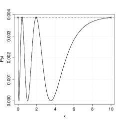
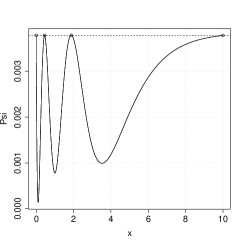
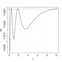
$\sigma^{2}=0$                         $\sigma^{2}=0.1$                      $\sigma^{2}=0.2$
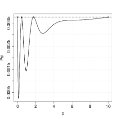
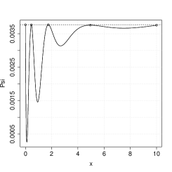
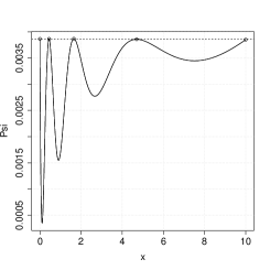
$\sigma^{2}=0.285$                        $\sigma^{2}=0.3$                     $\sigma^{2}=0.4$

Figure 1: The function on the left hand side of inequality (2.6) in the equivalence Theorem 2.1 for the numerically calculated Bayesian $T$-optimal discriminating designs. The competing regression models are given in (4.8).

4.2 Bayesian $T$-optimal discrimination designs for dose finding studies

Non-linear regression models have also numerous applications in dose response studies, where they are used to describe the dose response relationship. In these and similar situations the first step of the data analysis consists in the identification of an appropriate model, and the design of experiment should take this task into account. For example, for modeling the dose response relationship of a Phase II clinical trial Pinheiro et al., (2006) proposed the following plausible models

$$\eta_{1}(x,\theta_{1})=\theta_{1,1}+\theta_{1,2}x;$$

(4.11) $$\eta_{2}(x,\theta_{2})=\theta_{2,1}+\theta_{2,2}x(\theta_{2,3}-x);$$

$$\eta_{3}(x,\theta_{3})=\theta_{3,1}+\theta_{3,2}x/(\theta_{3,3}+x);$$

$$\eta_{4}(x,\theta_{4})=\theta_{4,1}+\theta_{4,2}/(1+\exp(\theta_{4,3}-x)/\theta_{4,4});$$

where the designs space (dose range) is given by the interval $\mathcal{X}=[0,500]$. In this reference some prior information regarding the parameters for the models is also provided, that is

$$\overline{\theta}_{1}=(60,0.56),\;\overline{\theta}_{2}=(60,7/2250,600),\;\overline{\theta}_{3}=(60,294,25),\;\ \overline{\theta}_{4}=(49.62,290.51,150,45.51).$$

Locally optimal discrimination designs for the models in (4.11) have been determined by Braess and Dette, (2013) in the case $p_{i,j}=1/6$, $(1\leq j<i\leq 4)$, which means that the resulting local $T$-optimality criterion (2.4) consists of $6$ model comparisons.
We begin with an illustration of the new methodology developed in Section 3 calculating again the locally $T$-optimal discriminating design for this scenario. The proposed algorithm needs only four iterations for the calculation of a design, say $\xi_{4}$, which has at least efficiency

$$\mathrm{Eff}_{T_{\mathrm{P}}}(\xi_{4})=\frac{T_{\mathrm{P}}(\tilde{\xi}_{4})}{\sup_{\zeta}T_{\mathrm{P}}(\zeta)}~{}\geq~{}0.999.$$

The function $\Psi(\cdot,\xi_{1})$ after the first iteration is displayed in Figure 2, where we used the same starting design as in Braess and Dette, (2013). The support points of $\ \xi_{1}$ are shown as circles and we can see that function $\Psi(x,\xi_{1})$ attains one and the same value, which is represented with dotted line, for all support points. We finally note that the algorithm proposed in Braess and Dette, (2013) needs $9$ iterations to find a design with the same efficiency.

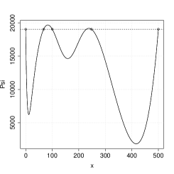
Figure 2: The function $\Psi(\cdot,\xi_{1})$ after the first iteration of Algorithm 3.2

We now investigate Bayesian $T$-optimal discriminating designs for a similar situation. For the sake of a transparent representation we only specify a prior distribution of the four-dimensional parameter $\overline{\theta}_{4}$ for the calculation of the discriminating design, while $\overline{\theta}_{2}$ and $\overline{\theta}_{3}$ are considered as fixed. In order to obtain a design which is robust with respect to model misspecification we chose a prior discrete prior with $81$ points in $\mathbb{R}^{4}$. More precisely, the support points of the prior distribution are given by the points

(4.12) $$\big{\{}\mu_{e_{1},e_{2},e_{3},e_{4}}~{}|~{}e_{1},e_{2},e_{3},e_{4}\in\{-1,0,1\}\big{\}},$$

where

$$\mu_{e_{1},e_{2},e_{3},e_{4}} =(\mu_{1}+e_{1}\sigma,\mu_{2}+e_{2}\sigma,\mu_{3}+e_{3}\sigma,\mu_{4}+e_{4}\sigma),$$

$$\mu =(\mu_{1},\mu_{2},\mu_{3},\mu_{4})=(49.62,290.51,150,45.51),$$

and different values for $\sigma^{2}$ are considered. The weights at the corresponding points are proportional (normalized such that their sum is $1$) to

(4.13) $$\frac{1}{(2\pi\sigma^{2})^{2}}\exp\Big{(}\frac{||\mu_{e_{1},e_{2},e_{3},e_{4}}-\mu||_{2}^{2}}{2\sigma^{2}}\Big{)}~{},~{}~{}e_{1},e_{2},e_{3},e_{4}\in\{-1,0,1\},$$

where $||\cdot||_{2}$ denotes the Euclidean norm. The resulting Bayesian optimality criterion (2.11) consist of $246$ model comparisons. In this case the method of Braess and Dette, (2013) fails to find the Bayesian $T$-optimal discriminating design. Bayesian $T$-optimal discriminating designs have been calculated by the new Algorithm 3.2 for various values of $\sigma^{2}$ and the results are shown in Table 2. A typical determination of the optimal design takes between $0.09$ seconds (in the case $\sigma^{2}=0$) and $7.8$ seconds (in the case $\sigma^{2}=37^{2}$) CPU time on a standard PC. The algorithm using the procedure described in Section 3.2 in Step 2 requires between $0.75$ seconds (in the case $\sigma^{2}=0$) and $37.1$ seconds (in the case $\sigma^{2}=37^{2}$) CPU time. For small values the Bayesian $T$-optimal discriminating designs are supported at $4$ points including the boundary of the design space. The smaller (larger) interior support point is increasing (decreasing) if $\sigma^{2}$ is increasing. For larger values of $\sigma^{2}$ even the number of support points of the optimal design increases. For example, if $\sigma^{2}=35^{2}$ or $37^{2}$ the Bayesian $T$-optimal discriminating design has $5$ or $6$ points (including the boundary points of the design space). These observations are in line with the theoretical finding of Braess and Dette, (2007) who showed that the number of support points of Bayesian $D$-optimal designs can become arbitrarily large with an increasing variability in the prior distribution. The corresponding functions from the equivalence Theorem 2.1 are shown in Figure 3.

$\sigma^{2}$	optimal design	$\sigma^{2}$	optimal design
0	$\begin{matrix}0.000&78.783&241.036&500.0\\ 0.255&0.213&0.357&0.175\end{matrix}$	$33^{2}$	$\begin{matrix}0.000&92.692&222.735&500.0\\ 0.260&0.240&0.344&0.156\end{matrix}$
$20^{2}$	$\begin{matrix}0.000&84.467&234.134&500.0\\ 0.257&0.225&0.351&0.167\end{matrix}$	$35^{2}$	$\begin{matrix}0.000&91.743&129.322&221.118&500.0\\ 0.260&0.214&0.036&0.336&0.154\end{matrix}$
$30^{2}$	$\begin{matrix}0.000&91.029&225.713&500.0\\ 0.259&0.237&0.345&0.159\end{matrix}$	$37^{2}$	$\begin{matrix}0.000&89.881&129.590&170.306&220.191&500.0\\ 0.260&0.170&0.091&0.019&0.310&0.150\end{matrix}$

Table 2: Bayesian $T$-optimal discriminating designs for the models in (4.11). The weights in the criterion (2.10) are given by $p_{i,j}=1/6$; $1\leq i<j\leq 4$ and the support and masses of the prior distribution are defined by (4.12) and (4.13), respectively.

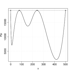
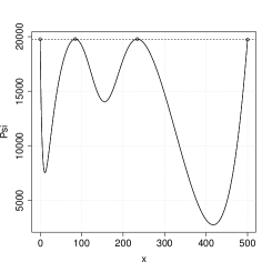
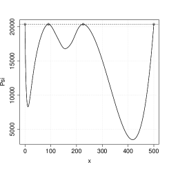
$\sigma^{2}=0$                        $\sigma^{2}=20$                     $\sigma^{2}=30$
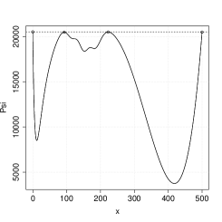
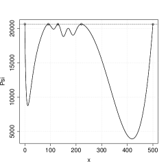
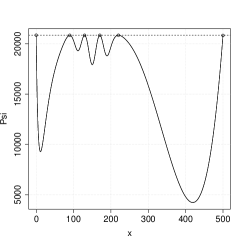
$\sigma^{2}=33$                        $\sigma^{2}=35$                     $\sigma^{2}=37$

Figure 3: The function on the left-hand side of inequality (2.6) in the equivalence Theorem 2.1 for the numerically calculated Bayesian $T$-optimal discriminating designs. The competing regression models are given in (4.11).

Acknowledgements. Parts of this work were done during a visit of the second author at the Department of Mathematics, Ruhr-Universität Bochum, Germany. The authors would like to thank M. Stein who typed this manuscript with considerable technical expertise. The work of H. Dette and V. Melas was supported by the Deutsche Forschungsgemeinschaft (SFB 823: Statistik nichtlinearer dynamischer Prozesse, Teilprojekt C2). The research of H. Dette reported in this publication was also partially supported by the National Institute of General Medical Sciences of the National Institutes of Health under Award Number R01GM107639. The content is solely the responsibility of the authors and does not necessarily represent the official views of the National Institutes of Health. V. Melas was also partially supported by Russian Foundation of Basic Research (Project 12.01.00747a).

5 Proofs

5.1 An auxiliary result

Lemma 5.1

Let $\varphi(v,y)$ be a twice continuously differentiable function of two variables $v\in\mathcal{V}\subset\mathbb{R}^{k}$ and $y\in\mathcal{Y},$ where $\mathcal{Y}$ is a compact set. Denote by ${\mathcal{Y}^{*}}$ the set of all points where the minimum $\min_{y\in\mathcal{Y}}\varphi(v,y)$ is attained and let $q\in\mathbb{R}^{k}$ be an arbitrary direction. Then

(5.1) $$\frac{\partial\min_{y\in{\mathcal{Y}^{*}}}\varphi(v,y)}{\partial q}=\min_{y\in{\mathcal{Y}^{*}}}\frac{\partial\varphi(v,y)}{\partial q}.$$

Proof.  See Pshenichny, (1971), p. 75.

5.2 Proofs

Proof of Theorem 2.2. Assume without loss of generality that $p_{i,j}>0$ for all $i,j=1,\dots,\nu$. Let $\xi^{*}$ denote any locally $T$-optimal discriminating design and let $\theta=(\theta_{i,j})_{i,j=1,\dots,\nu}$ denote the vector consisting of all $\theta_{i,j}\in\Theta_{i,j}(\xi^{*})$. We introduce the function

(5.2) $$\varphi(x,\theta) =\sum_{i,j=1}^{\nu}p_{i,j}\big{[}\eta_{i}(x,\overline{\theta}_{i})-\eta_{j}(x,{\theta}_{i,j})\big{]}^{2}$$

and consider the product measure

(5.3) $$\mu(d\theta)=\prod_{i,j=1,\ldots,\nu}\mu_{i,j}(d\theta_{i,j}),$$

where $\mu_{ij}$ are measures on the sets ${\Theta}_{i,j}^{*}(\xi^{*})$ defined by (2.5). Similarly, we define $\mu^{*}(d\theta)=\prod_{i,j=1,\ldots,\nu}\mu_{i,j}^{*}(d\theta_{i,j})$ as the product measure of the measures $\mu^{*}_{i,j}$ in Theorem 2.1. From this result we have

$$T_{\mathrm{P}}(\xi^{*}) \geq \sup_{\zeta}\int_{\mathcal{X}}\int_{\Theta^{*}(\xi^{*})}\varphi(x,\theta)\mu^{*}(d\theta)\zeta(dx)$$

$$\geq \inf_{\mu}\sup_{\zeta}\int_{\mathcal{X}}\int_{\Theta^{*}(\xi^{*})}\varphi(x,\theta)\mu(d\theta)\zeta(dx)=\sup_{\zeta}\inf_{\mu}\int_{\mathcal{X}}\int_{\Theta^{*}(\xi^{*})}\varphi(x,\theta)\mu(d\theta)\zeta(dx),$$

where the $\sup$ and $\inf$ are calculated in the class of designs $\zeta$ on $\mathcal{X}$ and product measures $\mu$ on $\Theta^{*}(\xi^{*})=\otimes_{i,j=1}^{\nu}\Theta_{i,j(\xi^{*})}^{*}$, respectively. It now follows that the characterizing inequality (2.6) in Theorem 2.1 is equivalent to the inequality

$$\sup_{\zeta}Q(\zeta,\xi^{*})\leq T_{\mathrm{P}}(\xi^{*}).$$

Consequently, any non-optimal design must satisfy the opposite inequality. $\Box$

Proof of Corollary 2.3: Let $\xi$ denote a design such that $T_{\mathrm{P}}(\xi)>0$ and recall the definition of the set $\Theta_{ij}^{*}(\xi)$ in (2.5). We consider for a vector $\theta=(\theta_{i,j})_{i,j=1,\ldots,\nu}\in\Theta^{*}(\xi)=\otimes_{i,j=1,\ldots,\nu}\Theta_{i,j}^{*}(\xi)$, the function $\varphi$ is defined in (5.2) and product measures $\mu(d\theta)$ of the form (5.3) on $\Theta^{*}(\xi)$. Now the well known minimax theorem and the definition of the function $Q$ in (2.7) yields

$$\max_{x\in\mathcal{X}}\Psi(x,\xi) = \inf_{\mu}\max_{x\in\mathcal{X}}\int_{\Theta^{*}(\xi)}\varphi(x,\theta)\mu(d\theta)=\inf_{\mu}\sup_{\zeta}\int_{\mathcal{X}}\int_{\Theta^{*}(\xi)}\varphi(x,\theta)\mu(d\theta)\zeta(dx)$$

$$= \sup_{\zeta}\inf_{\mu}\int_{\mathcal{X}}\int_{\Theta^{*}(\xi)}\varphi(x,\theta)\mu(d\theta)\zeta(dx)=\sup_{\zeta}\inf_{\theta\in\Theta^{*}(\xi)}\int\varphi(x,\theta)\zeta(dx)=\sup_{\zeta}Q(\zeta,\xi),$$

where the infimum is calculated with respect to all measures $\mu$ of the form (5.3) and the supremum is calculated with respect to all experimental designs $\zeta$ on $\mathcal{X}$. Note that $\mathcal{X}$ is compact by assumption and it can be checked that the set $\Theta^{*}(\xi)$ is also compact as a closed subset of a compact set. Consequently all suprema and infima are achieved and there exists a design $\zeta^{*}$ supported at the set of local maxima of the function $\Psi(x,\xi)$, such that

$$Q(\zeta^{*},\xi)=\sup_{\zeta}Q(\zeta,\xi)=\max_{x\in\mathcal{X}}\Psi(x,\xi).$$

The assertion of Corollary 2.3 now follows from Theorem 2.2. $\Box$

Proof of Theorem 3.3: Obviously, the inequality

$$T_{\mathrm{P}}(\{\mathcal{S}_{[s]},\omega_{[s]}\})\leq T_{\mathrm{P}}(\{\mathcal{S}_{[s+1]},\omega_{[s+1]}\})$$

holds for all $s$ as optimization with respect to $\omega$ occurs on a larger set. Moreover, the sequence $T_{\mathrm{P}}(\xi_{s})$ is bounded from above by $T_{\mathrm{P}}(\xi^{*})$ and has a limit, which is denoted by $T^{**}_{\mathrm{P}}$. Consequently, there exists a subsequence of designs, say $\xi_{s_{j}},j=1,2,\ldots$ converging to a design, say $\xi^{**}$. Note that $T_{P}$ is upper semi-continuous as the infimum of continuous functions, which implies $T_{\mathrm{P}}(\xi^{**})=T^{**}_{\mathrm{P}}$. Now, assume that $T_{\mathrm{P}}(\xi^{**})<T_{\mathrm{P}}(\xi^{*})$, then $\xi^{**}$ is not locally $T$-optimal and by Theorem 2.2 there exists a constant $\delta>0$ such that

$${\sup_{\zeta}Q(\zeta,\xi^{**})-T_{\mathrm{P}}(\xi^{**})=2\delta},$$

where the function $Q$ is defined in (2.7). Therefore for sufficiently large $j$, say, $j\geq N$ we obtain (using again the lower semi-continuity of $\sup_{\zeta}Q(\zeta,\xi)$) that

$$\sup_{\zeta}Q(\zeta,{\xi}_{s_{j}})-T_{\mathrm{P}}(\xi_{s_{j}})>\delta,$$

whenever $j\geq N$. Note that by construction the sequence $(T_{\mathrm{P}}(\xi_{s}))_{s\in\mathbb{N}}$ is increasing and therefore

(5.4) $$T_{\mathrm{P}}({\xi}_{s_{j+1}})-T_{\mathrm{P}}(\xi_{s_{j}})\geq T_{\mathrm{P}}(\xi_{s_{j}+1})-T_{\mathrm{P}}(\xi_{s_{j}}).$$

In order to estimate the right hand side we consider for $j\geq N$ and $\alpha\in[0,1]$ the design

$$\tilde{\xi}_{s_{j+1}}(\alpha)=(1-\alpha){\xi}_{s_{j}}+\alpha\zeta_{j},$$

where $\zeta_{j}$ is the measure for which the function $Q(\zeta,{\xi}_{s_{j}})$ attains its maximal value in the class of all experimental designs supported at the local maxima of the function $\Psi(x,{\xi}_{s_{j}})$, and define

$$\alpha_{s_{j+1}}=\operatorname*{arg\,max}_{0\leq\alpha\leq 1}T_{\mathrm{P}}(\tilde{\xi}_{s_{j+1}}(\alpha)).$$

By construction of ${\xi}_{s_{j}+1}$ is the best design supported at $\mbox{supp}({\xi}_{s_{j}})\cup\mbox{supp}(\zeta_{j})$, and (5.4) yields

(5.5) $$T_{\mathrm{P}}({\xi}_{s_{j+1}})\geq T_{\mathrm{P}}({\xi}_{s_{j}+1})\geq T_{\mathrm{P}}(\tilde{\xi}_{s_{j+1}}(\alpha_{s_{j+1}})).$$

We introduce the notations $h(j,\alpha)=T_{\mathrm{P}}(\tilde{\xi}_{s_{j}}(\alpha))$, and note that

$$\frac{\partial T_{\mathrm{P}}(\tilde{\xi}_{s_{j+1}}(\alpha))}{\partial\alpha}\Big{|}_{\alpha=0}=Q(\zeta_{j},{\xi}_{s_{j}})-T_{\mathrm{P}}({\xi}_{s_{j}})=\sup_{\zeta}Q(\zeta,{\xi}_{s_{j}})-T_{\mathrm{P}}({\xi}_{s_{j}})>\delta.$$

A Taylor expansion gives

$$h(j+1,\alpha_{s_{j+1}})-h(j+1,0)= \max_{\alpha\in[0,1]}\big{[}T_{\mathrm{P}}(\tilde{\xi}_{s_{j+1}}(\alpha))-T_{\mathrm{P}}(\tilde{\xi}_{s_{j+1}}(0))\big{]}$$

$$\geq \max_{\alpha\in[0,1]}\Big{[}\alpha\frac{\partial T_{\mathrm{P}}(\tilde{\xi}_{s_{j+1}}(\alpha))}{\partial\alpha}\Big{|}_{\alpha=0}-\frac{1}{2}\alpha^{2}K\Big{]}>\max_{\alpha\in[0,1]}\Big{[}\alpha\delta-\frac{1}{2}\alpha^{2}K\Big{]}=\frac{\delta^{2}}{2K},$$

where $K$ is an absolute upper bound of the second derivative. Therefore it follows from (5.5) that

$$T_{\mathrm{P}}(\xi_{s_{j+1}})-T_{\mathrm{P}}(\xi_{s_{j}}) \geq T_{\mathrm{P}}(\xi_{s_{j}+1})-T_{\mathrm{P}}(\xi_{s_{j}})$$

$$\geq T_{\mathrm{P}}(\tilde{\xi}_{s_{j+1}}(\alpha_{s_{j+1}}))-T_{\mathrm{P}}(\xi_{s_{j}})=h(j+1,\alpha_{s_{j+1}})-h(j+1,0)\geq\frac{\delta^{2}}{2K}.$$

which gives for $L>N+1$

$$T_{\mathrm{P}}(\xi_{s_{L}})-T_{\mathrm{P}}(\xi_{s_{N}})=\sum_{j=N}^{L-1}\big{[}T_{\mathrm{P}}(\xi_{s_{j+1}})-T_{\mathrm{P}}(\xi_{s_{j}})\big{]}\geq\left[L-N\right]\frac{\delta^{2}}{2K}.$$

The left hand side of this inequality converges to the finite value $T(\xi^{**})-T(\xi_{s_{N}})$ as $L\to\infty$, while the right hand side converges to infinity. Therefore we obtain a contradiction to our assumption $T_{\mathrm{P}}(\xi^{**})<T_{\mathrm{P}}(\xi^{*})$, which proves the assertion of Theorem 3.3.

Proof of Lemma 3.4: Fix $t\in\{1,\dots,n\}$ and note that $w_{t}=1-\sum^{n}_{\ell=1,\ell\neq t}w_{\ell}$. Under Assumptions 2.1 and 2.2 we obtain by formula (5.1)

$$\frac{\partial g(\omega)}{\partial\omega_{k}} =\sum_{i,j=1}^{\nu}p_{i,j}\big{[}\eta_{i}(x_{k},\overline{\theta}_{i})-\eta_{j}(x_{k},\widehat{\theta}_{i,j}(\omega))\big{]}^{2}-\sum_{i,j=1}^{\nu}p_{i,j}\big{[}\eta_{i}(x_{t},\overline{\theta}_{i})-\eta_{j}(x_{t},\widehat{\theta}_{i,j}(\omega))\big{]}^{2}$$

The condition $\frac{\partial g(\omega)}{\partial\omega_{k}}=0,\;k=1,\dots,n,\;k\neq t$ is the necessary condition for weight optimality and consequently it follows from the definition of the function $\Psi(x,\overline{\xi}_{s+1})$ that this function attains one and the same value for all support points of the design $\overline{\xi}_{s+1}$.

Proof of Theorem 3.6: The proof is similar to the proof of Theorem 3.3. Denote

$$h(\gamma,\alpha)=g(\overline{\omega}_{(\gamma)}(\alpha)),$$

where the vector $\overline{\omega}_{(\gamma)}(\alpha^{*})$ is calculated at the $\gamma$th iteration. Since the sequence $g(\omega_{(\gamma)})$ is bounded and increasing (by construction) it converges to some limit, say $g^{**}$. Consequently there exists a subsequence of vector of weights, say $\overline{\omega}_{(\gamma_{j})},j=1,2,\ldots$ converging to a vector, say $\overline{\omega}^{**}$. Note that $g$ is upper semi-continuous as the infimum of continuous functions, which implies $g(\overline{\omega}^{**})=g^{**}$. Now, assume that $g(\overline{\omega}^{**})<g(\omega^{*})$, then it follows by an application of Theorem 2.1 with $\mathcal{X}=\{x_{1},\ldots,x_{n}\}$ that there exists a constant $\delta>0$ such that

$$\frac{\partial g(\overline{\omega}(\alpha))}{\partial\alpha}\Bigl{|}_{\alpha=0}=2\delta>0.$$

Here the vector $\overline{\omega}(\alpha)$ is defined in the same way as $\overline{\omega}_{(\gamma)}(\alpha)$, where $\omega_{(\gamma)}$ is replaced by $\omega=\omega^{**}$. Therefore for sufficiently large $j$, say, $j\geq N$ we obtain (using the lower semi-continuity of ${g}$) that $h(\gamma_{j},0)>\delta,$ and a Taylor expansion yields

$$h(\gamma_{j+1},\alpha^{*}_{(\gamma_{j+1})})-h(s_{j},\alpha^{*}_{(\gamma_{j})}))\geq\max_{\alpha}\Big{(}\alpha\frac{\partial g(\overline{\omega}(\alpha))}{\partial\alpha}-\frac{1}{2}\alpha^{2}K\Big{)}=\frac{\delta^{2}}{2K},$$

where $\alpha^{*}_{(\gamma_{j})}$ is the value $\alpha^{*}$ from the $\gamma_{j}$th iteration and $K$ is an absolute upper bound of the second derivative. Using the same arguments as in the proof of Theorem 3.3 we obtain a contradiction, which proves the assertion of the theorem.

References

- Atkinson et al., (2007) Atkinson, A., Donev, A., and Tobias, R. (2007). Optimum Experimental Designs, with SAS (Oxford Statistical Science Series). Oxford University Press, USA, 2nd edition.
- Atkinson, (2008) Atkinson, A. C. (2008). Examples of the use of an equivalence theorem in constructing optimum experimental designs for random-effects nonlinear regression models. Journal of Statistical Planning and Inference, 138(9):2595–2606.
- Atkinson et al., (1998) Atkinson, A. C., Bogacka, B., and Bogacki, M. B. (1998). - and -optimum designs for the kinetics of a reversible chemical reaction. Chemometrics and Intelligent Laboratory Systems, 43:185–198.
- (4) Atkinson, A. C. and Fedorov, V. V. (1975a). The designs of experiments for discriminating between two rival models. Biometrika, 62:57–70.
- (5) Atkinson, A. C. and Fedorov, V. V. (1975b). Optimal design: Experiments for discriminating between several models. Biometrika, 62:289–303.
- Braess and Dette, (2007) Braess, D. and Dette, H. (2007). On the number of support points of maximin and Bayesian -optimal designs in nonlinear regression models. Annals of Statistics, 35:772–792.
- Braess and Dette, (2013) Braess, D. and Dette, H. (2013). Optimal discriminating designs for several competing regression models. Annals of Statistics, 41(2):897–922.
- Chaloner and Verdinelli, (1995) Chaloner, K. and Verdinelli, I. (1995). Bayesian experimental design: A review. Statistical Science, 10(3):273–304.
- Chernoff, (1953) Chernoff, H. (1953). Locally optimal designs for estimating parameters. Annals of Mathematical Statistics, 24:586–602.
- Dette, (1997) Dette, H. (1997). Designing experiments with respect to “standardized” optimality criteria. Journal of the Royal Statistical Society, Ser. B, 59:97–110.
- Dette and Haller, (1998) Dette, H. and Haller, G. (1998). Optimal designs for the identification of the order of a Fourier regression. Annals of Statistics, 26:1496–1521.
- Dette et al., (2012) Dette, H., Melas, V. B., and Shpilev, P. (2012). T-optimal designs for discrimination between two polynomial models. Annals of Statistics, 40(1):188–205.
- Dette et al., (2013) Dette, H., Melas, V. B., and Shpilev, P. (2013). Robust -optimal discriminating designs. Annals of Statistics, 41(4):1693–1715.
- Foo and Duffull, (2011) Foo, L. K. and Duffull, S. (2011). Optimal design of pharmacokinetic-pharmacodynamic studies. In Bonate, P. L. and Howard, D. R., editors, Pharmacokinetics in Drug Development, Advances and Applications. Springer.
- Han and Chaloner, (2003) Han, C. and Chaloner, K. (2003). - and -optimal designs for exponential regression models used in pharmacokinetics and viral dynamics. Journal of Statistical Planning and Inference, 115:585–601.
- Kiefer, (1974) Kiefer, J. (1974). General equivalence theory for optimum designs (approximate theory). Annals of Statistics, 2(5):849–879.
- López-Fidalgo et al., (2007) López-Fidalgo, J., Tommasi, C., and Trandafir, P. C. (2007). An optimal experimental design criterion for discriminating between non-normal models. Journal of the Royal Statistical Society, Series B, 69:231–242.
- Pinheiro et al., (2006) Pinheiro, J., Bretz, F., and Branson, M. (2006). Analysis of dose-response studies: Modeling approaches. In Ting, N., editor, Dose Finding in Drug Development, pages 146–171. Springer-Verlag, New York.
- Pronzato and Walter, (1985) Pronzato, L. and Walter, E. (1985). Robust experimental design via stochastic approximation. Mathematical Biosciences, 75:103–120.
- Pshenichny, (1971) Pshenichny, B. N. (1971). Necessary Conditions of an Extremum. Marcel Dekker, New York.
- Pukelsheim, (2006) Pukelsheim, F. (2006). Optimal Design of Experiments. SIAM, Philadelphia.
- Ratkowsky, (1990) Ratkowsky, D. (1990). Handbook of Nonlinear Regression Models. Dekker, New York.
- Song and Wong, (1999) Song, D. and Wong, W. K. (1999). On the construction of -optimal designs. Statistica Sinica, 9:263–272.
- Stigler, (1971) Stigler, S. (1971). Optimal experimental design for polynomial regression. Journal of the American Statistical Association, 66:311–318.
- Tommasi, (2009) Tommasi, C. (2009). Optimal designs for both model discrimination and parameter estimation. Journal of Statistical Planning and Inference, 139:4123–4132.
- Tommasi and López-Fidalgo, (2010) Tommasi, C. and López-Fidalgo, J. (2010). Bayesian optimum designs for discriminating between models with any distribution. Computational Statistics & Data Analysis, 54(1):143–150.
- Ucinski and Bogacka, (2005) Ucinski, D. and Bogacka, B. (2005). -optimum designs for discrimination between two multiresponse dynamic models. Journal of the Royal Statistical Society, Ser. B, 67:3–18.
- Wiens, (2009) Wiens, D. P. (2009). Robust discrimination designs, with Matlab code. Journal of the Royal Statistical Society, Ser. B, 71:805–829.
- Yang et al., (2013) Yang, M., Biedermann, S., and Tang, E. (2013). On optimal designs for nonlinear models: A general and efficient algorithm. Journal of the American Statistical Association, 108:1411–1420.
- Yu, (2010) Yu, Y. (2010). Monotonic convergence of a general algorithm for computing optimal designs. The Annals of Statistics, 38(3):1593–1606.