Effects of Gapless Bosonic Fluctuations on Majorana Fermions in Atomic Wire Coupled to a Molecular Reservoir

Abstract

We discuss the effects of quantum and thermal fluctuations on the Majorana edge states in a topological atomic wire coupled to a superfluid molecular gas with gapless excitations. We find that the coupling between the Majorana edge states remains exponentially decaying with the length of the wire, even at finite temperatures smaller than the energy gap for bulk excitations in the wire. This exponential dependence is controlled solely by the localization length of the Majorana states. The fluctuations, on the other hand, provide the dominant contribution to the preexponential factor, which increases with temperature and the length of the wire. More important is that thermal fluctuations give rise to a decay of an initial correlation between Majorana edge states to its stationary value after some thermalization time. This stationary value is sensitive to the temperature and to the length of the wire, and, although vanishing in the thermodynamic limit, can still be feasible in a mesoscopic system at sufficiently low temperatures. The thermalization time, on the other hand, is found to be much larger than the typical time scales in the wire, and is sufficient for quantum operations with Majorana fermions before the temperature-induced decoherence sets in.

I Introduction

Majorana fermions Wilczek2009 (or Ising anyons) are probably the simplest example of non-Abelian anyons - quantum objects with exchange operations resulting in non-commuting unitary transformations on the space of degenerate ground states (see, for example AnyonReview0 ; AnyonReview1 ; AnyonReview2 and references therein). The emerging non-Abelian statistics has not only fundamental importance as an alternative to the canonical bosonic and fermionic ones, but also provides tools for topological quantum computation AnyonReview0 ; TQC1 ; TQC2 ; TQC3 ; TQC4 . In many-body systems, non-Abelian anyons can emerge as quasi-particles in topological ordered states PfQHE ; Read2000 ; Anyon1 . One of the simplest systems exhibiting Majorana fermions, is a one-dimensional (1D) topological superconductor – a system of 1D spinless fermions with a nearest-neighbor (in a lattice realization Kitaev ) or $p$-wave (in a continuous one Cheng ) pairing amplitude, in which Majorana fermions appear as edge states. A variety of physical setups have been proposed for the realization of the corresponding Hamiltonians both in solid-state structures Majreview1 ; Majreview2 ; Majreview3 ; MajCMP0 ; MajCMP1 ; MajCMP2 ; MajCMP12 ; MajCMP3 and in systems of ultracold atoms and molecules LiangJiang ; Nascimbene ; MajAtom2 ; MajAtom3 ; MajAtom10 ; MajAtom11 . Based on these proposals, recent experiments MajEx1 ; MajEx2 ; MajEx30 ; MajEx3 ; Churchill2013 ; Finck2013 ; MajEx4 provide strong evidences for the existence of Majorana states and make an important step toward an experimental demonstration of the existence of objects with non-Abelian statistics.

A key element of most of the considered setups for the realization of Majorana states is a coupling of the one-dimensional fermions to a reservoir which serves a source of pairs to generate an effective $p$-wave (or nearest-neighbor) pairing amplitude. In the realizations with solid-state systems MajCMP0 ; MajCMP1 ; MajCMP2 ; MajCMP12 ; MajCMP3 , the reservoir is a bulk superconductor and the coupling is due to the proximity effect. In the atom-molecule realizations LiangJiang ; Nascimbene , the reservoir is a cloud of molecular BEC and the coupling involves some molecular dissociation mechanism. The two reservoirs, being absolutely similar on a mean-field level in providing the $p$-wave pairing amplitude for fermions, have very different low-energy excitations and, therefore, their quantum and thermal fluctuations behave differently. In a solid state superconducting reservoir, one has gapped single-particle excitations, whereas the excitations in a superfluid molecular reservoir are gapless collective modes – Bogoliubov sound. As a result, the correlations between fluctuations in a solid-state superconducting reservoir are short-range, and their account do not change the mean-field result – the coupling between Majorana edge states remains exponentially decaying with the distance between them Dloss . On the other hand, the decay of correlations between fluctuations in a molecular superfluid reservoir follows a power law, raising the question of their effects on the mean-field results.

In this paper we discuss the effects of quantum and thermal fluctuations in a molecular superfluid reservoir on the properties of Majorana fermion edge states in a finite one-dimension system of fermionic atoms in a lattice. Our consideration is based on a generic microscopic Hamiltonian describing a coupled system of atoms in the lattice and a surrounded superfluid molecular cloud.

The paper is organized as follows. In Sec. II we describe our microscopic model and show the emergence of the Kitaev Hamiltonian for fermions in the lattice. The properties of the Majorana edge states, as well as fermionic excitations in the wire and bosonic ones in the reservoir are discussed in Sec. III. The interactions between the excitations are the topic of Sec. IV. The analysis of their effects on the properties of the Majorana fermions at zero temperature is presented in Secs. V and VI, and at finite temperatures in Sec. VII. The consequences and the proposals for optimal experimental conditions are briefly discussed in Sec. VIII. Technical details are given in two Appendices: In Appendix A we present a scenario leading to our microscopic Hamiltonian. This can be viewed as a new proposal for experimental realization of Majorana edge states, as well as an example demonstrating the capability to control the microscopic Hamiltonian of the topological wire under experimental conditions. Appendix B contains analytical solution of the Bogoliubov-de Gennes equations for the wave function and the energy of the Majorana fermions in a finite Kitaev wire with open boundary conditions, and the calculations of several correlation functions in the bulk of the wire.

II Microscopic model

We consider a system of single-component fermionic atoms in a one-dimensional (1D) optical lattice (wire) coupled to a Bose-condensed gas of homonuclear molecules (reservoir) made of two fermionic atoms in different internal states BlochDalibardZwerger . The most essential for our purposes part of this coupling is a process converting a molecule from the reservoir into two atoms in the wire (and vice versa). An underlying physical mechanism of this conversion could be, for example, radio-frequency assisted dissociation LiangJiang or tunneling Nascimbene . In Appendix A, we present another possible mechanism involving Raman transitions between different internal states of atoms. To be more specific, we consider the Hamiltonian

$$H={H}_{\mathrm{BEC}}+{H}_{\mathrm{L}}+{H}_{\mathrm{conv}}+{H}_{\mathrm{int}},$$ (1)

where ${H}_{\mathrm{BEC}}$ is the Hamiltonian for the molecular reservoir,

$${H}_{\mathrm{BEC}}=\int d\mathbf{r}\hat{\phi}^{{\dagger}}\left(-\frac{\hbar^{2}}{2m}\nabla^{2}-\mu_{\mathrm{M}}+\frac{g_{M}}{2}\hat{\phi}^{{\dagger}}\hat{\phi}\right)\hat{\phi},$$ (2)

with $\hat{\phi}(\mathbf{r})$ being the field operator of diatomic molecules with the mass $m=2m_{a}$ and the binding energy $E_{b}=\hbar^{2}/m_{a}a_{s}^{2}$, where $a_{s}$ is the scattering length between the  atoms forming the molecule, $g_{\mathrm{M}}=4\pi\hbar^{2}a_{\mathrm{M}}/m$ is the molecular coupling constant with $a_{\mathrm{M}}$ being the molecule-molecule scattering length ($a_{\mathrm{M}}\approx 0.6a_{s}$, see PetrovSolomonSchlyapnikov ; PetrovSolomonSchlyapnikov1 ), and $\mu_{\mathrm{M}}$ is the molecular chemical potential. In the following, we will consider the regime of weak interaction $n_{\mathrm{M}}a_{\mathrm{M}}^{3}<1$, where $n_{\mathrm{M}}$ is the density of molecules.

The second term in Hamiltonian (1)

$$H_{\mathrm{L}}=\sum_{j}\left[-J\left(\hat{a}_{j}^{{\dagger}}\hat{a}_{j+1}+\hat{a}_{j+1}^{\dagger}\hat{a}_{j}\right)-\mu_{0}\hat{a}_{j}^{{\dagger}}\hat{a}_{j}\right],$$ (3)

describes fermionic atoms in the wire. Here $\hat{a}_{j}$ and $\hat{a}_{j}^{{\dagger}}$ are fermionic annihilation and creation operators on a site $j$ , respectively, $J$ is the hopping amplitude, and $\mu_{0}$ is the fermionic chemical potential.

The conversion of a molecule from the reservoir into two atoms in the wire is described by the third term in Hamiltonian (1)

$${H}_{\mathrm{conv}}=\sum_{j}\int d\mathbf{r}\left[K_{j}(\mathbf{r})\hat{a}_{j}^{{\dagger}}\hat{a}_{j+1}^{{\dagger}}\hat{\phi}\left(\mathbf{r}\right)+\text{h.c}.\right].$$ (4)

Here, the explicit form of the amplitude $K_{j}(\mathbf{r})$ relies on the specific realization of the conversion mechanism (see, for example, Ref. Nascimbene or Appendix A).

Finally, the last term in Hamiltonian (1)

$$H_{\mathrm{int}}=\sum_{j}\int d\mathbf{r}g_{j}(\mathbf{r})\hat{a}_{j}^{{\dagger}}\hat{a}_{j}\hat{\phi}^{{\dagger}}(\mathbf{r})\hat{\phi}(\mathbf{r})$$ (5)

describes a short-range interaction between atoms and molecules (assuming their spatial overlap) with $g_{j}(\mathbf{r})=g_{a\mathrm{M}}w^{2}(\mathbf{r}-\mathbf{r}_{j})$, where $g_{aM}$ is the atom-molecule interaction and $w(\mathbf{r}-\mathbf{r}_{j})$ is the Wannier function centered on the site $j$ in the wire.

Note that in writing the Hamiltonians ${H}_{\mathrm{conv}}$ and ${H}_{\mathrm{int}}$, we take into account only the nearest-neighbour and on-site terms, respectively, assuming the condition $a_{s}<a$ that the size of the molecule $a_{s}$ is smaller than the lattice spacing $a$. Intuitively, this condition arises naturally in optimizing the conversion, because too small or too large molecules will lead to smaller overlap of their wave function with Wannier functions on different sites of the wire, and therefore, results in a smaller conversion amplitude $K$ (see, for example, Appendix A).

Assuming zero temperature at the moment, we will treat the Hamiltonian (1) within the Bogoliubov framework by decomposing the molecular field operator $\hat{\phi}(\mathbf{r})$ into a mean-field part and quantum fluctuations, $\hat{\phi}(\mathbf{r})=\phi_{0}(\mathbf{r})+\delta\hat{\phi}(\mathbf{r})$, with $\phi_{0}(\mathbf{r})=\langle\hat{\phi}(\mathbf{r})\rangle$ being the mean-field condensate function and $\delta\hat{\phi}(\mathbf{r})$ representing the quantum fluctuations respectively. With this decomposition, Hamiltonian (1) can be recast into a sum of three components

$$H=H_{\mathrm{BMF}}(\phi_{0})+{H}_{\mathrm{K}}(\phi_{0})+H_{\mathrm{f}},$$ (6)

where

$$H_{\mathrm{BMF}}=\int d\mathbf{r}\phi_{0}^{\ast}\left(-\frac{\hbar^{2}}{2m}\nabla^{2}-\mu_{\mathrm{M}}+\frac{g_{M}}{2}|\phi_{0}|^{2}\right)\phi_{0}$$ (7)

is the mean-field BEC Hamiltonian,

$$H_{\mathrm{K}}=\sum_{j=1}^{L-1}(\!-\!J\hat{a}_{j}^{{\dagger}}\hat{a}_{j+1}+{\ \Delta_{\phi_{0}}}\hat{a}_{j}^{{\dagger}}\hat{a}_{j+1}^{{\dagger}}+\text{h.c.})-\sum_{j=1}^{L}\mu_{f}\hat{a}_{j}^{{\dagger}}\hat{a}_{j}$$ (8)

is the Kitaev Hamiltonian Kitaev for fermionic atoms with the pairing amplitude

$${\Delta_{\phi_{0}}=|\Delta|}e^{i\theta}=\int d\mathbf{r}K_{j}\left(\mathbf{r})\phi_{0}(\mathbf{r}\right)$$ (9)

and the renormalized chemical potential for fermions

$$\mu_{f}=\mu_{0}+\int d\mathbf{r}g_{j}(\mathbf{r})\left|\phi_{0}\left(\mathbf{r}\right)\right|^{2}.$$ (10)

The third component in Eq. (6), Hamiltonian $H_{\mathrm{f}}$, contains the effects of bosonic fluctuations $\delta\hat{\phi}$.

In Eq. (8), we have shown the emergence of the Kitaev Hamiltonian $H_{K}$, which has a gap parameter defined in terms of the mean-field condensate function $\phi_{0}$. The Gross-Pitaevskii (GP) equation for the condensate wave function $\phi_{0}$ can be found by demanding that the term in $H_{f}$, which is linear in the fluctuations of the molecular field $\delta\hat{\phi}$ only, vanishes. The resulting GP equation reads

$$\left(-\frac{\hbar^{2}\nabla^{2}}{2m}+g_{\text{M}}\left|\phi_{0}(\mathbf{r})\right|^{2}\right)\phi_{0}(\mathbf{r})+\sum_{j}\left[K_{j}^{\ast}(\mathbf{r})\left\langle\hat{a}_{j+1}\hat{a}_{j}\right\rangle_{H_{\mathrm{K}}}+g_{j}(\mathbf{r})\phi_{0}(\mathbf{r})\left\langle\hat{a}_{j}^{{\dagger}}\hat{a}_{j}\right\rangle_{H_{\mathrm{K}}}\right]=\mu_{\text{M}}\phi_{0}(\mathbf{r}),$$ (11)

where $\langle\ldots\rangle_{H_{\mathrm{K}}}$ denotes the expectation value with respect to the ground state of the Hamiltonian ${H}_{\mathrm{K}}(\phi_{0})$ in Eq. (8). Equation (11) thus determines the condensate wave function $\phi_{0}$ self-consistently.

With the condensate wave function $\phi_{0}(\mathbf{r})$ satisfying Eq. (11), the Hamiltonian $H_{\mathrm{f}}$ reduces to the sum,

$$H_{\mathrm{f}}=H_{\mathrm{ph}}+H_{\mathrm{c}}+H_{\mathrm{ph-ph}},$$ (12)

which consist of the Bogoliubov Hamiltonian for phonons $H_{\mathrm{ph}}$ (the part quadratic in $\delta\hat{\phi}$), the interaction of phonons with fermionic excitations $H_{\mathrm{c}}$, and the phonon-phonon interactions $H_{\mathrm{ph-ph}}$. More explicitly,

$$H_{\mathrm{ph}}=\int d\mathbf{r}\left\{\delta\hat{\phi}^{{\dagger}}\left[-\frac{\hbar^{2}\nabla^{2}}{2m}-\mu_{\mathrm{M}}+2g\left|\phi_{0}\right|^{2}+\sum_{j}g_{j}\left\langle\hat{a}_{j}^{{\dagger}}\hat{a}_{j}\right\rangle_{{H}_{\mathrm{K}}}\right]\delta\hat{\phi}+g_{M}\left(\phi_{0}^{2}\delta\hat{\phi}^{{\dagger}}\delta\hat{\phi}^{{\dagger}}+\phi_{0}^{\ast 2}\delta\hat{\phi}\delta\hat{\phi}\right)\right\},$$ (13)

and

$$H_{\mathrm{c}}=H_{\mathrm{c}}^{(3)}+H_{\mathrm{c}}^{(4)}$$ (14)

with

$$H_{\mathrm{c}}^{(3)} =\sum_{j}\int d\mathbf{r}\Big{\{}K_{j}(\mathbf{r})(\hat{a}_{j}^{{\dagger}}\hat{a}_{j+1}^{{\dagger}}-\langle\hat{a}_{j}^{{\dagger}}\hat{a}_{j+1}^{{\dagger}}\rangle_{H_{\mathrm{K}}})\delta\hat{\phi}(\mathbf{r})+\text{ h.c.}$$

$$+g_{j}(\mathbf{r})(\hat{a}_{j}^{{\dagger}}\hat{a}_{j}-\langle\hat{a}_{j}^{{\dagger}}\hat{a}_{j}\rangle_{H_{\mathrm{K}}})(\delta\hat{\phi}^{{\dagger}}\phi_{0}\!+\!\text{h.c.})\Big{\}},$$ (15)

$$H_{\mathrm{c}}^{(4)} =\sum_{j}\int d^{3}\mathbf{r}g_{j}(\mathbf{r})(\hat{a}_{j}^{{\dagger}}\hat{a}_{j}-\langle\hat{a}_{j}^{{\dagger}}\hat{a}_{j}\rangle_{H_{\mathrm{K}}})\delta\hat{\phi}^{{\dagger}}(\mathbf{r})\delta\hat{\phi}(\mathbf{r}),$$ (16)

where $\hat{a}_{j}^{{\dagger}}\hat{a}_{j+1}^{{\dagger}}-\langle\hat{a}_{j}^{{\dagger}}\hat{a}_{j+1}^{{\dagger}}\rangle$ and $\hat{a}_{j}^{{\dagger}}\hat{a}_{j}-\langle\hat{a}_{j}^{{\dagger}}\hat{a}_{j}\rangle$ represent fermionic fluctuations (this form is equivalent to the normal ordering of the fermionic quasiparticle operators). The phonon-phonon interaction Hamiltonian $H_{\mathrm{ph-ph}}$ contains cubic and quartic in $\delta\hat{\phi}$ contributions which can be easily obtained from Eq. (6). Here we do not write down $H_{\mathrm{ph-ph}}$ explicitly, because the corresponding terms contain no coupling to the fermions and result only in the renormalization of the bosonic excitations (phonon modes) defined by the Bogoliubov Hamiltonian (13). This renormalization is not important for our purposes, and we neglect the Hamiltonian $H_{\mathrm{ph-ph}}$ assuming that the Hamiltonian $H_{\mathrm{ph}}$ already contains the “true ”excitations in the molecular BEC. As a result, in describing the system we limit ourselves to the effective Hamiltonian

$${H}_{\mathrm{eff}}={H}_{\mathrm{K}}+H_{\mathrm{ph}}+H_{\mathrm{c}},$$ (17)

accompanied by the GP equation (11) for the self-consistent determination of the molecular condensate wave function $\phi_{0}(\mathbf{r})$. In the Hamiltonian ${H}_{\mathrm{eff}}$, the first two (quadratic) terms $H_{\mathrm{K}}$ and ${H}_{\mathrm{ph}}$ describe fermionic and bosonic quasiparticles, respectively, and the last term ${H}_{\mathrm{c}}$ corresponds to interactions between them.

III Fermionic and Bosonic quasiparticles

Let us first consider the properties of fermionic and bosonic quasiparticles described by the quadratic Hamiltonians (8) and (13), respectively. The properties of the Kitaev Hamiltonian ${H}_{\mathrm{K}}$ in Eq. (8) for $1D$ spinless fermions in the lattice are well-known Kitaev . We summarize them here to make the presentation self-contained, and to create a ‘reference’ point for future discussion of the effects of quantum fluctuations.

Being quadratic in fermionic operators of the form

$${H}_{\mathrm{K}}=-\frac{1}{2}\sum\limits_{i,j}t_{ij}(\hat{a}_{i}^{{\dagger}}\hat{a}_{j}+\text{h.c.})+\frac{1}{2}\sum\limits_{i,j}(\Delta_{ij}\hat{a}_{i}^{{\dagger}}\hat{a}_{j}^{{\dagger}}+\text{h.c.}),$$

with obvious expressions for $t_{ij}$ and $\Delta_{ij}=-\Delta_{ji}$ written down from Eq. (8), the Hamiltonian ${H}_{\mathrm{K}}$ can be diagonalized by the Bogoliubov transformation

$$\hat{a}_{j}=\sum_{m}\left(u_{j,m}\hat{\alpha}_{m}+\upsilon_{j,m}^{\ast}\hat{\alpha}_{m}^{{\dagger}}\right),$$ (18)

where the quasiparticle (excitation) fermionic annihilation and creation operators $\hat{\alpha}_{m}$ and $\hat{\alpha}_{m}^{{\dagger}}$ obey canonical anticommutation relations. The amplitudes $u_{j,m}$ and $\upsilon_{j,m}$ satisfy the conditions $\sum_{j}(u_{j,m_{1}}^{\ast}u_{j,m_{2}}+\upsilon_{j,m_{1}}^{\ast}\upsilon_{j,m_{2}})=\delta_{m_{1}m_{2}}$ and $\sum_{j}(u_{j,m_{1}}\upsilon_{j,m_{2}}+\upsilon_{j,m_{1}}u_{j,m_{2}})=0$, and can be found from the Bogoliubov-de-Gennes (BDG) equations

$$\sum_{j}\left(-t_{ij}u_{j,m}+\Delta_{ij}\upsilon_{j,m}\right) =E_{m}u_{i,m},$$

$$\sum_{j}\left(t_{ij}\upsilon_{j,m}+\Delta_{ji}^{\ast}u_{j,m}\right) =E_{m}\upsilon_{i,m}$$

with the quasiparticle energy $E_{m}\geq 0$. The diagonal form of the Hamiltonian reads

$${H}_{\mathrm{K}}=E_{0}+\sum_{m}E_{m}\hat{\alpha}_{m}^{{\dagger}}\hat{\alpha}_{m},$$ (19)

where $E_{0}=-\sum_{j,m}E_{m}\left|\upsilon_{j,m}\right|^{2}$ is the energy of the ground state $\left|0\right\rangle$ defined by the conditions $\hat{\alpha}_{j,m}\left|0\right\rangle=0$ for all $\hat{\alpha}_{j,m}$.

A remarkable feature of the Kitaev Hamiltonian ${H}_{\mathrm{K}}$ is the existence of the topological phase for $|\mu_{f}|<2J$ Kitaev , in which a robust ‘zero-energy’ fermionic edge mode ($m=M$, to be specific) emerges with an energy $E_{M}$ vanishing exponentially with the system size $L$, while other modes (with $m=\nu\neq M$) are gapped $E_{\nu}>\left|\Delta\right|$. In the thermodynamic limit $L\rightarrow\infty$, the presence of such edge modes results in the degeneracy of the ground state: The states $\left|0\right\rangle$ and $\hat{\alpha}_{M}^{{\dagger}}|0\rangle$ have the same energy. Moreover, although having different fermionic parity, the two states cannot be distinguished by local measurements in the bulk of the wire. This is because they differ by the occupation of the fermionic edge mode and, therefore, have the same local correlations in the bulk.

The edge character of the ‘zero-energy’ mode and its connection to Majorana fermions can be revealed by writing the corresponding annihilation operator in the form $\hat{\alpha}_{M}=(\hat{\gamma}_{L}+i\hat{\gamma}_{R})/2$, where

$$\hat{\gamma}_{L}=\hat{\alpha}_{M}+\hat{\alpha}_{M}^{{\dagger}}=\sum_{j}\left[(u_{jM}^{\ast}+\upsilon_{jM})\hat{a}_{j}+(u_{jM}+\upsilon_{jM}^{\ast})\hat{a}_{j}^{{\dagger}}\right],$$

and

$$\hat{\gamma}_{R}=-i(\hat{\alpha}_{M}-\hat{\alpha}_{M}^{{\dagger}})=-i\sum_{j}\left[(u_{jM}^{\ast}-\upsilon_{jM})\hat{a}_{j}+(\upsilon_{jM}^{\ast}-u_{jM})\hat{a}_{j}^{{\dagger}}\right],$$

are two Hermitian Majorana operators satisfying the conditions $\hat{\gamma}_{L(R)}=\hat{\gamma}_{L(R)}^{{\dagger}}$, $\hat{\gamma}_{L(R)}^{2}=1$, and $\gamma_{L}\gamma_{R}=-\gamma_{R}\gamma_{L}$. It turns out that (see Ref. Kitaev and Appendix B for details)

$$f_{Lj}\equiv u_{jM}+\upsilon_{jM}^{\ast}\approx 2\left|A\right|\rho^{j}\sin(j\theta)\sim e^{-ja/l_{M}}$$ (20)

and

$$f_{Rj}\equiv u_{jM}-\upsilon_{jM}^{\ast}\approx 2\left|A\right|\rho^{L+1-j}\sin[(L+1-j)\theta]\sim e^{-(L+1-j)a/l_{M}},$$ (21)

where we assume $4(J^{2}-\left|\Delta\right|^{2})-\mu^{2}>0$ such that

$$\left|A\right|=\sqrt{\frac{\left|\Delta\right|(4J^{2}-\mu^{2})}{J(4J^{2}-4\left|\Delta\right|^{2}-\mu^{2})}},\;\rho=\sqrt{\frac{J-\left|\Delta\right|}{J+\left|\Delta\right|}}<1,\;\cos\theta=\frac{-\mu}{2\sqrt{J^{2}-\left|\Delta\right|^{2}}}$$

and the Majorana localization length (for details and for the general case see Appendix B)

$$l_{M}=\frac{a}{\ln\rho^{-1}}.$$ (22)

The localization length $l_{M}$ also enters the expression for the energy of the mode $\hat{\alpha}_{M}$,

$$E_{M}\approx\left|\Delta\right|\frac{4J^{2}-\mu^{2}}{J(J+\left|\Delta\right|)}\rho^{L}\left|\frac{\sin[(L+1)\theta]}{\sin\theta}\right|\sim e^{-La/l_{M}},$$ (23)

which becomes exponentially small for $L\gg l_{M}/a$ [see Eq. (130)]. The above expressions show that the fermionic ‘zero-energy’ mode $\hat{\alpha}_{M}$ represents a non-local fermion associated with two spatially separated Majorana operators $\hat{\gamma}_{L}$ and $\hat{\gamma}_{R}$ localized at the opposite edges of the wire. The following form of the Hamiltonian $H_{\mathrm{K}}$

$$H_{\mathrm{K}} =E_{0\mathrm{f}}+E_{M}\hat{\alpha}_{M}^{{\dagger}}\hat{\alpha}_{M}+\sum_{\nu}E_{\nu}\hat{\alpha}_{\nu}^{{\dagger}}\hat{\alpha}_{\nu}$$ (24)

$$=E_{0\mathrm{f}}+\frac{1}{2}E_{M}+\frac{i}{2}E_{M}\hat{\gamma}_{L}\hat{\gamma}_{R}+\sum_{\nu}E_{\nu}\hat{\alpha}_{\nu}^{{\dagger}}\hat{\alpha}_{\nu},$$

emphasizes this special ‘zero-energy’ edge mode $\hat{\alpha}_{M}$ and its connection to the Majorana edge modes $\hat{\gamma}_{L}$ and $\hat{\gamma}_{R}$, as compared to the gapped bulk excitations $\hat{\alpha}_{\nu}$ with energies $E_{\nu}>\left|\Delta\right|$ (for details on the bulk gapped modes see B). Note that the energy $E_{M}$ of the fermionic mode can also be viewed as the coupling between the corresponding Majorana modes $\hat{\gamma}_{L}$ and $\hat{\gamma}_{R}$.

The properties of bosonic quasi-particles are described by the Hamiltonian $H_{\mathrm{ph}}$, Eq. (13), which can be diagonalized by using the standard bosonic Bogoliubov transformation

$$\delta\hat{\phi}(\mathbf{r})=\sum_{\gamma}[\tilde{u}_{\gamma}(\mathbf{r})\hat{b}_{\gamma}-\tilde{\upsilon}_{\gamma}^{\star}(\mathbf{r})\hat{b}_{\gamma}^{{\dagger}}]$$ (25)

in terms of bosonic quasiparticle (phonon) operators $\hat{b}_{\gamma}$, where $\tilde{u}_{\gamma}$ and $\tilde{\upsilon}_{\gamma}$ are the solutions of the corresponding Bogoliubov-de-Gennes equations. The diagonalized Hamiltonian reads

$$H_{\mathrm{ph}}=E_{0\mathrm{ph}}+\sum_{\gamma}\epsilon_{\gamma}\hat{b}_{\gamma}^{{\dagger}}\hat{b}_{\gamma},$$ (26)

where $E_{0\mathrm{ph}}$ is the quasiparticle ground state energy, and $\epsilon_{\gamma}$ is the quasiparticle spectrum. In general, the interaction with fermions results in a spatially non-uniform condensate wave function $\phi_{0}(\mathbf{r})\neq\mathrm{const}$, as well as in the appearance of a position-dependent external potential in Eq. (13) for $H_{\mathrm{ph}}$. As a consequence, bosonic excitations are not characterized by the momentum, and their wave functions are not plane waves anymore. The problem of finding the coefficients $\tilde{u}_{\gamma}(\mathbf{r})$ and $\tilde{\upsilon}_{\gamma}(\mathbf{r})$ of the Bogoliubov transformation (25) and the corresponding eigen-energies $\epsilon_{\gamma}$ in this case can only be addressed numerically. In the considered case of a large (compare to the wire) BEC and weak coupling, the interaction with fermions in the wire generates quantitatively small effects on bosonic excitations in the reservoir. We will therefore neglect them and consider a spatially homogeneous condensate with $\phi_{0}(\mathbf{r})=\sqrt{n_{\mathrm{M}}}$ and bosonic excitations characterized by the wave vector $\mathbf{q}$. The corresponding wave functions are then plane waves, $[\tilde{u}_{\mathbf{q}}(\mathbf{r}),\tilde{\upsilon}_{\mathbf{q}}(\mathbf{r})]=(\tilde{u}_{q},\tilde{\upsilon}_{q})V^{-1/2}\exp(i\mathbf{qr})$, such that

$$\delta\hat{\phi}(\mathbf{r})=\frac{1}{\sqrt{V}}\sum_{\mathbf{q}}(\tilde{u}_{q}\hat{b}_{\mathbf{q}}-\tilde{\upsilon}_{q}\hat{b}_{-\mathbf{q}}^{{\dagger}})\exp(i\mathbf{qr}),$$ (27)

where $\tilde{u}_{q}^{2}(\tilde{v}_{q}^{2})=\left[\left(\epsilon_{q}^{0}+g_{\mathrm{M}}n_{\mathrm{M}}\right)/\epsilon_{q}\pm 1\right]/2$ with $\epsilon_{q}=\sqrt{\epsilon_{q}^{0}\left(\epsilon_{q}^{0}+2g_{\mathrm{M}}n_{\mathrm{M}}\right)}$ and $\epsilon_{q}^{0}=\hbar^{2}q^{2}/2m$. As usual, for small wave vectors $q\lesssim\xi_{\text{BEC}}^{-1}$, where $\xi_{\text{BEC}}=\hbar/\sqrt{mg_{\mathrm{M}}n_{\mathrm{M}}}$ is the coherence length of the condensate, the excitations are phonons $\epsilon_{q}=\hbar cq$ with the sound velocity $c=\sqrt{g_{\mathrm{M}}n_{\mathrm{M}}/m}$.

IV Interaction between quasiparticles

Let us now analyze the effects of the interaction $H_{\mathrm{c}}$ between fermions excitations in the lattice and fluctuations in the reservoir (phonons) on the properties of the “zero-energy”fermionic edge mode $\hat{\alpha}_{M}$. We will be primarily interested in corrections to the energy $E_{M}$ of the mode, see Eq. (24).

By using the Bogoliubov transformations (18) and (25), the Hamiltonian (17) reads

$$H_{\mathrm{eff}}=E_{0}+H_{0}+{H}_{\mathrm{c}}^{(3)}+{H}_{\mathrm{c}}^{(4)},$$ (28)

where $E_{0}$ is the ground state energy of the system,

$$H_{0}=\sum_{m}E_{m}\hat{\alpha}_{m}^{{\dagger}}\hat{\alpha}_{m}+\sum_{\mathbf{q}}\epsilon_{q}\hat{b}_{\mathbf{q}}^{{\dagger}}\hat{b}_{\mathbf{q}}$$ (29)

describes fermionic and bosonic excitations, and the terms

$${H}_{\mathrm{c}}^{(3)}=\sum_{\mathbf{q}}\sum_{m,n}\Big{[}O_{\mathbf{q}mn}^{(n)}\hat{\alpha}_{m}^{{\dagger}}\hat{\alpha}_{n}\hat{b}_{\mathbf{q}}^{{\dagger}}+\text{ h.c.}+(O_{\mathbf{q}mn}^{(a1)}\hat{\alpha}_{m}\hat{\alpha}_{n}+O_{\mathbf{q}mn}^{(a2)}\hat{\alpha}_{m}^{{\dagger}}\hat{\alpha}_{n}^{{\dagger}})\hat{b}_{\mathbf{q}}^{{\dagger}}+\text{h.c.}\Big{]},$$ (30)

and

$${H}_{\mathrm{c}}^{(4)}=\sum_{\mathbf{q}_{1},\mathbf{q}_{2}}\sum_{m,n}\Big{[}V_{\mathbf{q}_{1}\mathbf{q}_{2}mn}\hat{\alpha}_{m}^{{\dagger}}\hat{\alpha}_{n}\hat{b}_{\mathbf{q}_{1}}^{{\dagger}}\hat{b}_{\mathbf{q}_{2}}+\ldots\Big{]},$$ (31)

provide interactions between them, where the dots in ${H}_{\mathrm{c}}^{(4)}$ denote all other possible terms containing two fermionic and two bosonic operators with the corresponding matrix elements. The Hamiltonians (30) and (31) describe interactions between fermionic and bosonic quasiparticles: The first line in ${H}_{\mathrm{c}}^{(3)}$ corresponds to the emission (absorption) of a phonon by a fermionic quasiparticle accompanied by a change of its quantum states, $n\rightarrow m$ , while the second line describes processes involving emission (absorption) of a phonon and annihilation (creation) of a pair of fermionic quasiparticles. The Hamiltonian ${H}_{\mathrm{c}}^{(4)}$ contains processes with creation (annihilation) of two fermionic excitations and emission (absorption) of two phonons.

We will consider the effects of the interaction Hamiltonians ${H}_{\mathrm{c}}^{(3)}$ and ${H}_{\mathrm{c}}^{(4)}$ in the weak coupling case $n_{M}a_{s}^{3}<1$ by using systematic perturbation expansion in this small parameter. In what follows, we limit ourselves to the lowest order contributions: the first order in ${H}_{\mathrm{c}}^{(4)}$ and the second order in ${H}_{\mathrm{c}}^{(3)}$.

The interactions between fermionic and bosonic quasiparticles results in renormalization of their properties. More specifically, the interactions modify the energies $E_{m}$ and $\epsilon_{q}$ of quasiparticles (adding also imaginary parts responsible for the decay of quasiparticles when it is allowed by conservation laws). In the considered case of a weak coupling between the wire and the reservoir, the renormalization of bosonic and gapped fermionic bulk excitations ($m=\nu$) does not lead to any qualitative change in their properties, and we will ignore it. On the other hand, the properties of the “zero-energy ”edge mode ($m=M$), in particular, its exponentially small energy $E_{M}$, can be modified substantially due to the coupling to the gapless phonon modes. Below we will focus on the effects of the effects of gapless bosonic excitations on the Majorana fermions.

We start our analysis with calculating the effects of ${H}_{\mathrm{c}}^{(4)}$. The leading first-order contribution can be obtained by averaging over the bosonic fields in Eq. (16), $\delta\hat{\phi}^{{\dagger}}(\mathbf{\ r})\delta\hat{\phi}(\mathbf{r})\rightarrow\left\langle\delta\hat{\phi}^{{\dagger}}(\mathbf{r})\delta\hat{\phi}(\mathbf{r})\right\rangle_{H_{\mathrm{ph}}}=n_{\text{M}}^{\prime}$ with $n_{\text{M}}^{\prime}$ being the condensate depletion, which yields (we omit an unimportant constant)

$$H_{\mathrm{c}}^{(4)}\rightarrow\left\langle H_{\mathrm{c}}^{(4)}\right\rangle_{H_{\mathrm{ph}}}=\sum_{j}\hat{a}_{j}^{{\dagger}}\hat{a}_{j}\int d^{3}\mathbf{r}g_{j}(\mathbf{r})n_{\text{M}}^{\prime}.$$

This term provides the renormalization of the fermionic chemical potential $\mu_{f}$ in the Kitaev Hamiltonian by replacing the condensate density $\left|\phi_{0}\right|^{2}$ with the total molecular density $n_{\text{M}}=\left|\phi_{0}\right|^{2}+n_{\text{M}}^{\prime}$ in Eq. (10) for $\mu_{f}$. The corresponding changes can be trivially taken into account by staring with the renormalized $\mu_{f}$ in the initial Kitaev Hamiltonian (8).

The interaction Hamiltonian ${H}_{\mathrm{c}}^{(3)}$ contributes in the second order of the perturbation theory. To select the contributions in ${H}_{\mathrm{c}}^{(3)}$ that couple the “zero-energy”edge mode $\hat{\alpha}_{M}$ to other modes, we write the fermionic operator $\hat{a}_{j}$ in the form

$$\hat{a}_{j} =u_{jM}\hat{\alpha}_{M}+\upsilon_{jM}^{\ast}\hat{\alpha}_{M}^{{\dagger}}+\hat{a}_{j}^{\prime}$$

$$=\frac{1}{2}[f_{Lj}+f_{Rj}]\hat{\alpha}_{M}+\frac{1}{2}[f_{Lj}-f_{Rj}]\hat{\alpha}_{M}^{{\dagger}}+\hat{a}_{j}^{\prime},$$

where we use Eqs. (20) and (21) to express the amplitudes $u_{j,M}$ and $v_{j,M}$ in terms of the wave functions of the Majorana edge modes $f_{Lj}$ and $f_{Rj}$ (we take real $f_{Lj}$ and $f_{Rj}$), and $\hat{a}_{j}^{\prime}$ contains the operators $\hat{\alpha}_{\nu}$ and $\hat{\alpha}_{\nu}^{{\dagger}}$ of the gapped modes only. The Hamiltonian ${H}_{\mathrm{c}}^{(3)}$ then takes the form

$${H}_{\mathrm{c}}^{(3)} ={H}_{\mathrm{c1}}^{(3)}+{H}_{\mathrm{c2}}^{(3)}+{H}_{\mathrm{c3}}^{(3)}$$

$$=\sum_{\mathbf{q}}\left[O_{\mathbf{q}MM}^{(n)}\hat{\alpha}_{M}^{{\dagger}}\hat{\alpha}_{M}\hat{b}_{\mathbf{q}}^{{\dagger}}+\text{h.c.}\right]$$

$$+\sum_{\mathbf{q},\nu}\Big{[}(O_{\mathbf{q}\nu M}^{(n1)}\hat{\alpha}_{\nu}^{{\dagger}}\hat{\alpha}_{M}+O_{\mathbf{q}\nu M}^{(n2)}\hat{\alpha}_{\nu}\hat{\alpha}_{M}^{{\dagger}}+2O_{\mathbf{q}\nu M}^{(a1)}\hat{\alpha}_{\nu}\hat{\alpha}_{M}+2O_{\mathbf{q}\nu M}^{(a2)}\hat{\alpha}_{\nu}^{{\dagger}}\hat{\alpha}_{M}^{{\dagger}})\hat{b}_{\mathbf{q}}^{{\dagger}}+\text{h.c.}\Big{]}$$

$$+\sum_{\mathbf{q},\nu,\mu}\left[(O_{\mathbf{q}\nu\mu}^{(n)}\hat{\alpha}_{\nu}^{{\dagger}}\hat{\alpha}_{\mu}\!+\!O_{\mathbf{q}\nu\mu}^{(a1)}\hat{\alpha}_{\nu}\hat{\alpha}_{\mu}\!+\!O_{\mathbf{q}\nu\mu}^{(a2)}\hat{\alpha}_{\nu}^{{\dagger}}\hat{\alpha}_{\mu}^{{\dagger}})\hat{b}_{\mathbf{q}}^{{\dagger}}\!+\!\text{h.c.}\right],$$ (32)

where the terms in the second line (the Hamiltonian ${H}_{c1}^{(3)}$) couple phonons to the “zero-energy”mode $\hat{\alpha}_{M}$, the terms in the third line (${H}_{\mathrm{c2}}^{(3)}$) correspond to the interaction of phonons with the mode $\hat{\alpha}_{M}$ and the gapped modes $\hat{\alpha}_{\nu}$, and the terms in the last line (${H}_{\mathrm{c3}}^{(3)}$) describe coupling of phonon to the gapped modes.

With the use of Eqs. (15), (20) and (21), it is easy to see that the matrix element $O_{\mathbf{q}MM}^{(n)}$ contains the products of the Majorana wave functions belonging to different edges,

$$O_{\mathbf{q}MM}^{(n)}=\frac{1}{\sqrt{V}}\int d\mathbf{re}^{-i\mathbf{qr}}\sum_{j}\left\{\frac{1}{2}[K_{j}(\mathbf{r})\tilde{\upsilon}_{q}-K_{j}^{\ast}(\mathbf{r})\tilde{u}_{q}](f_{Lj}f_{Rj+1}-f_{Rj}f_{Lj+1})+g_{j}(\mathbf{r})[\tilde{u}_{q}\phi_{0}-\tilde{\upsilon}_{q}\phi_{0}^{\ast}]f_{Lj}f_{Rj}\right\},$$

is exponentially small with the system size, $O_{\mathbf{q}MM}^{(n)}\sim\exp(-L/l_{M})\sim E_{M}$. As a result, the leading (second order) contribution of ${H}_{\mathrm{c1}}^{(3)}$ to $\delta E_{M}$ is proportional to $E_{M}^{2}$ and can be neglected. We therefore have to consider only the Hamiltonians ${H}_{\mathrm{c2}}^{(3)}$ and ${H}_{\mathrm{c3}}^{(3)}$.

The Hamiltonian ${H}_{\mathrm{c2}}^{(3)}$ can be conveniently written in the form

$${H}_{\mathrm{c2}}^{(3)}=(H_{L}^{(-)}+H_{R}^{(-)})\hat{\alpha}_{M}+(H_{L}^{(+)}+H_{R}^{(+)})\hat{\alpha}_{M}^{{\dagger}},$$ (33)

where

$$H_{L}^{(+)} =H_{L}^{(-)}=-H_{L}^{(+){\dagger}}$$

$$=\frac{1}{2}\sum_{jj^{\prime}}f_{Lj}\int d\mathbf{r}[-K_{jj^{\prime}}(\mathbf{r})\delta\hat{\phi}(\mathbf{r})\hat{a}_{j^{\prime}}^{\prime{\dagger}}+K_{jj^{\prime}}^{\ast}(\mathbf{r})\delta\hat{\phi}^{{\dagger}}(\mathbf{r})\hat{a}_{j^{\prime}}^{\prime}]+\frac{1}{2}\sum_{j}f_{Lj}\int d\mathbf{r}g_{j}(\mathbf{r})(\phi_{0}\delta\hat{\phi}^{{\dagger}}+\phi_{0}^{\ast}\delta\hat{\phi})(\hat{a}_{j}^{\prime{\dagger}}-\hat{a}_{j}^{\prime})$$ (34)

and

$$H_{R}^{(+)} =-H_{R}^{(-)}=H_{R}^{(+){\dagger}}$$

$$=\frac{1}{2}\sum_{jj^{\prime}}f_{Rj}\int d\mathbf{r}[-K_{jj^{\prime}}(\mathbf{r})\delta\hat{\phi}(\mathbf{r})\hat{a}_{j^{\prime}}^{\prime{\dagger}}-K_{jj^{\prime}}^{\ast}(\mathbf{r})\delta\hat{\phi}^{{\dagger}}(\mathbf{r})\hat{a}_{j^{\prime}}^{\prime}]-\frac{1}{2}\sum_{j}f_{Rj}\int d\mathbf{r}g_{j}(\mathbf{r})(\phi_{0}\delta\hat{\phi}^{{\dagger}}+\phi_{0}^{\ast}\delta\hat{\phi})(\hat{a}_{j}^{\prime{\dagger}}+\hat{a}_{j}^{\prime})$$ (35)

[here $K_{j_{1}j_{2}}(\mathbf{r})=-K_{j_{2}j_{1}}(\mathbf{r})\equiv K_{j_{1}}(\mathbf{r})\delta_{j_{2},j_{1}+1}$] contain the wave function of the left $f_{Lj}$ and of the right $f_{Rj}$ Majorana modes, respectively, and are linear in both bosonic operators of the reservoir $\delta\hat{\phi}(\mathbf{r})$ and $\delta\hat{\phi}^{{\dagger}}(\mathbf{r})$, and in fermionic operators of the gapped modes $\hat{a}_{j}^{\prime}$ and $\hat{a}_{j}^{\prime{\dagger}}$. The relations between the $+$ and $-$ operators suggest another form for ${H}_{\mathrm{c2}}^{(3)}$,

$${H}_{\mathrm{c2}}^{(3)}=\left(H_{L}^{(+)}-H_{R}^{(+)}\right)\hat{\alpha}_{M}+\left(H_{L}^{(+)}+H_{R}^{(+)}\right)\hat{\alpha}_{M}^{{\dagger}},$$ (36)

which will be used below for the analysis of different contributions to $\delta E_{M}$.

V Effects of interactions between quasiparticles. Zero temperature

In order to calculate the energy correction $\delta E_{M}$ to the energy $E_{M}$ resulting from the second line of Eq. (32), one has to compare the corrections to the energies of the ground state $\left|0\right\rangle$ and of the state $|M\rangle=\hat{\alpha}_{M}^{{\dagger}}|0\rangle$ in which only the edge mode is populated, given by

$$\delta E_{M}=\delta E_{|M\rangle}-\delta E_{|0\rangle}.$$

The corrections to the ground state energy originates from the processes with simultaneous creation and then annihilation of two fermionic excitations (the edge mode and a bulk one) and one phonon, described by the $O_{\mathbf{q}\nu M}^{(a2)}$-term, while the correction to the energy of the state $|M\rangle$ involves simultaneous annihilation of the edge-mode excitation and creation of a bulk fermionic excitation and a phonon, $O_{\mathbf{q}\nu M}^{(n1)}$-term, followed by the reverse process. Direct application of the perturbation theory yields

$$\delta E_{M}=\sum_{\mathbf{q},\nu}\frac{\left|O_{\mathbf{q}\nu M}^{(n1)}\right|^{2}}{E_{M}-(E_{\nu}+\epsilon_{q})}-\sum_{\mathbf{q},\nu}\frac{4\left|O_{\mathbf{q}\nu M}^{(a2)}\right|^{2}}{-(E_{M}+E_{\nu}+\epsilon_{q})}$$

$$\approx\sum_{\mathbf{q},\nu}\frac{4\left|O_{\mathbf{q}\nu M}^{(a2)}\right|^{2}\!-\!\left|O_{\mathbf{q}\nu M}^{(n1)}\right|^{2}}{E_{\nu}+\epsilon_{q}}\!-\!E_{M}\frac{4\left|O_{\mathbf{q}\nu M}^{(a2)}\right|^{2}\!+\!\left|O_{\mathbf{q}\nu M}^{(n1)}\right|^{2}}{(E_{\nu}\!+\!\epsilon_{q})^{2}}$$

$$=\delta E_{M}^{(1)}+\delta E_{M}^{(2)},$$ (37)

where in the second line we have neglected terms $\sim E_{M}^{2}/\Delta_{m}\ll E_{M}$. It should be mentioned that the Hamiltonian ${H}_{\mathrm{c3}}^{(3)}$ contributes equally to the energies of the two states and, hence, the corresponding contributions cancel each other. Note that the relevant intermediate states contain a phonon and a gapped bulk excitation such that $E_{\nu}+\epsilon_{q}>\left|\Delta\right|$ in the denominators in Eq. (37). Having also in mind that the matrix elements in the numerators involve the wave functions of the edge modes, we therefore could expect an exponential decay of $\delta E_{M}$ with the system size $L$.

Another form of the expression for $\delta E_{M}$ can be obtained by writing the matrix elements in the form [see Eqs. (32) and (36)]

$$O_{\mathbf{q}\nu M}^{(n1)} =\left\langle\mathbf{q}\nu\left|H_{L}^{(+)}-H_{R}^{(+)}\right|0\right\rangle,$$ (38)

$$2O_{\mathbf{q}\nu M}^{(a2)} =\left\langle\mathbf{q}\nu\left|H_{L}^{(+)}+H_{R}^{(+)}\right|0\right\rangle.$$ (39)

After straightforward calculations we then obtain the following expressions for $\delta E_{M}^{(1)}$ and $\delta E_{M}^{(2)}$

$$\delta E_{M}^{(1)} \approx 2\sum_{\mathbf{q},\nu}\frac{\left\langle\mathbf{0}\left|H_{R}^{(+)}{}^{{\dagger}}\right|\mathbf{q}\nu\right\rangle\left\langle\mathbf{q}\nu\left|H_{L}^{(+)}\right|0\right\rangle+\left\langle\mathbf{0}\left|H_{L}^{(+)}{}^{{\dagger}}\right|\mathbf{q}\nu\right\rangle\left\langle\mathbf{q}\nu\left|H_{R}^{(+)}\right|0\right\rangle}{E_{\nu}+\epsilon_{q}}=4\sum_{\mathbf{q},\nu}\frac{\operatorname{Re}\left\langle\mathbf{0}\left|H_{R}^{(+)}{}^{{\dagger}}\right|\mathbf{q}\nu\right\rangle\left\langle\mathbf{q}\nu\left|H_{L}^{(+)}\right|0\right\rangle}{E_{\nu}+\epsilon_{q}},$$ (40)

$$\delta E_{M}^{(2)} \approx-2E_{M}\sum_{\mathbf{q},\nu}\frac{\left|\left\langle\mathbf{q}\nu\left|H_{L}^{(+)}\right|0\right\rangle\right|^{2}+\left|\left\langle\mathbf{q}\nu\left|H_{R}^{(+)}\right|0\right\rangle\right|^{2}}{(E_{\nu}+\epsilon_{q})^{2}},$$ (41)

which can also be obtained by direct application of the perturbation theory with the interaction Hamiltonian ${H}_{\mathrm{c2}}^{(3)}$ given by Eq. (36).

The expressions (37) for $\delta E_{M}$ can be recast into a more transparent form in terms of correlation functions as

$$\delta E_{M}=-\frac{i}{\hbar}\int_{0}^{\infty}d\tau e^{-\delta\tau}\left\{\left\langle M\left|H_{\mathrm{c2I}}^{(3)}(\tau)H_{\mathrm{c2I}}^{(3)}(0)\right|M\right\rangle-\left\langle 0\left|H_{\mathrm{c2I}}^{(3)}(\tau)H_{\mathrm{c2I}}^{(3)}(0)\right|0\right\rangle\right\},$$ (42)

where $H_{\mathrm{c2I}}^{(3)}(\tau)$ is the interaction Hamiltonian ${H}_{\mathrm{c2}}^{(3)}$ in the interaction representation, $H_{\mathrm{c2I}}^{(3)}(\tau)=e^{iH_{0}\tau/\hbar}{H}_{\mathrm{c2}}^{(3)}e^{-iH_{0}\tau/\hbar}$,  and $\delta\rightarrow+0$. [Eq. (37) is recovered after inserting the complete set of intermediate state $|\mathbf{q}\nu\rangle$ with one bosonic and one gapped fermionic excitation.] This expression shows that the energy change $\delta E_{M}$ results entirely from the edges of the wire because, as it was mentioned above, all correlations in the bulk for the two states $|M\rangle$ and $|0\rangle$ are equal. After using the form of ${H}_{\mathrm{c2}}^{(3)}$ given by Eq. (36), the expression (42) can be rewritten as

$$\delta E_{M} =-\frac{i}{\hbar}\int_{0}^{\infty}d\tau e^{-\delta\tau}2\cos(\frac{E_{M}\tau}{\hbar})\left[\left\langle 0\left|H_{L}^{(+)}{}^{{\dagger}}e^{-\frac{i}{\hbar}H_{0}\tau}H_{R}^{(+)}\right|0\right\rangle+(L\leftrightarrow R)\right]$$

$$+\frac{i}{\hbar}\int_{0}^{\infty}d\tau e^{-\delta\tau}2i\sin(\frac{E_{M}\tau}{\hbar})\left[\left\langle 0\left|H_{L}^{(+)}{}^{{\dagger}}e^{-\frac{i}{\hbar}H_{0}\tau}H_{L}^{(+)}\right|0\right\rangle+(L\rightarrow R)\right],$$ (43)

which provides another form of Eqs. (40), and (41) for $\delta E_{M}^{(1)}$ and $\delta E_{M}^{(2)}$.

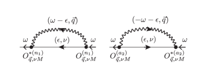
Figure 1: Feynman diagrams for normal contributions to the self-energy of the $\alpha$-mode at zero temperature. Solid lines correspond to gapped fermionic excitations in the wire and wavy lines to bosinic excitations in the molecular condensate.

The above results show that the correction to the energy of the $\alpha_{M}$ mode involve two different types of correlations: The contribution $\delta E_{M}^{(1)}$ involves long-range correlations between different edges, while the contribution $\delta E_{M}^{(2)}$ contains local correlations at the edges. As a result, the system-size dependence of $\delta E_{M}^{(2)}$ originates from the $L$-dependence of the energy $E_{M}$ of the mode, $\delta E_{M}^{(2)}\sim E_{M}\sim\exp(-La/l_{M})$, while the $L$-dependence of $\delta E_{M}^{(1)}$ results from the combined effect of the localization of the edge modes described by $l_{M}$, and of the short-range correlations in the bulk of the wire described by the coherence length $\xi_{\text{BCS}}=l_{M}$ (see Appendix B). We therefore also expect that the leading dependence of $\delta E_{M}^{(1)}$ on the system size is exponential, $\delta E_{M}^{(1)}\sim\exp(-La/l_{M})$.

An alternative derivation of the energy splitting $\delta E_{M}$ is based on the Green’s function technique (see, for example, Ref. Fetter ), which applies to both the zero temperature and finite temperature regime which we will discuss later. In the Green’s function approach, the energies of excitation correspond to the poles of the Green’s function considered as a function of the frequency $\omega$. The Green’s function for the “zero-energy”edge mode $\alpha_{M}$ is defined as

$$G_{M}(\tau) = -i\left\langle\mathrm{T}\{\alpha_{M}(\tau)\alpha_{M}^{{\dagger}}(0)\}\right\rangle$$

$$= \int\frac{d\varepsilon}{2\pi\hbar}G_{M}(\varepsilon)\exp(-\frac{i}{\hbar}\varepsilon\tau).$$

Here, $\mathrm{T}\{\alpha_{M}(\tau)\alpha_{M}^{{\dagger}}(0)\}$ is the time-ordered product of Heisenberg operators $\alpha_{M}(\tau)$ and $\alpha_{M}(0)=\alpha_{M}$, where the evolution is defined by the Hamiltonian ${H}^{(0)}+{H}_{\mathrm{c2}}^{(3)}+{H}_{\mathrm{c2}}^{(3)}$, and the averaging is over the exact ground state of this Hamiltonian. The Green’s function $G_{M}(\varepsilon)$ can be found from the Dyson equation

$$G_{M}^{-1}(\varepsilon)=G_{M}^{(0)-1}(\varepsilon)-\Sigma_{M}(\varepsilon)=\varepsilon-E_{M}-\Sigma_{M}(\varepsilon),$$

where $G_{M}^{(0)}(\varepsilon)=(\varepsilon-E_{M}+i0)^{-1}$ is the bare Green’s function and $\Sigma_{M}(\varepsilon)$ is the self-energy of the $\alpha$-mode, such that finding the renormalized energy of the $\alpha$ -mode reduces to solving the equation

$$\varepsilon-E_{M}-\Sigma_{M}(\varepsilon)=0.$$ (44)

At zero temperature and in the considered second-order of the perturbation theory, the self-energy $\Sigma_{M}(\varepsilon)$ results from only two normal (with one incoming and one outgoing lines of the $\alpha$-mode) contributions as illustrated in Fig. 1. There, the solid line corresponds to the bare Green’s function of a gapped fermionic excitation $G_{\nu}^{(0)}(\varepsilon)=(\varepsilon-E_{\nu}+i0)^{-1}$ and the wavy line to the bare bosonic excitation $D_{\mathbf{q}}^{(0)}(\varepsilon)=(\varepsilon-\epsilon_{q}+i0)^{-1}$. The corresponding analytic expression of $\Sigma_{M}(\varepsilon)=\Sigma_{M}^{(n)}(\varepsilon)$ reads

$$\Sigma_{M}(\varepsilon)=\sum_{\mathbf{q},\nu}\frac{\left|O_{\mathbf{q}\nu M}^{(n1)}\right|^{2}}{\varepsilon-(E_{\nu}+\epsilon_{q})}+\sum_{\mathbf{q},\nu}\frac{4\left|O_{\mathbf{q}\nu M}^{(a2)}\right|^{2}}{\varepsilon+E_{\nu}+\epsilon_{q}}.$$ (45)

After solving Eq. (44) to the lowest order in the perturbation,

$$\varepsilon\approx E_{M}+\Sigma_{M}^{(n)}(E_{M}),$$ (46)

we recover the expression (37) for $\delta E_{M}$.

It should be mentioned that the terms in $H_{\mathrm{c}}^{(3)}$ with matrix elements $O_{\mathbf{q}\nu M}^{(a1)}$ and $O_{\mathbf{q}\nu M}^{(a2)}$ [see Eq. (32)] generate in the second order also the “anomalous”terms with two $\alpha_{M}$-lines going out [$\Delta_{M}(\varepsilon)$, see Figs. 2(a) and 2(b)], or going in [$\Delta_{M}^{\ast}(\varepsilon)$, see Figs. 2(c) and 2 (d)], which contribute to the “anomalous”part of the self-energy $\Sigma_{M}^{(a)}(\varepsilon)=\left|\Delta_{M}(\varepsilon)\right|^{2}[\varepsilon+E_{M}+\Sigma_{M}^{(n)}(\varepsilon)]^{-1}$. These “anomalous”terms, however, are proportional to the frequency, $\Delta_{M}(\varepsilon)\sim$ $\varepsilon$ for small $\varepsilon$ (as a consequence of the Fermi-Dirac statistics) and, therefore, do not affect the leading second-order solution (46) or (37) of the equation (44). In other words, these frequency-proportional anomalous terms do not “open a gap”. This is in contrast to the standard pairing case where frequency-independent anomalous terms open a finite gap $\sim\left|\Delta\right|^{2}$ which does not depend on the size of the system.

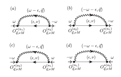
Figure 2: Feynman diagrams for the anomalous terms $\Delta_{M}$ [(a) and (b)] and $\Delta_{M}^{\ast}$ [(c) and (d)] for the $\alpha$-mode. Solid lines correspond to gapped fermionic excitations in the wire and wavy lines to bosinic excitations in the molecular condensate.

VI Evaluation of the energy correction

We now proceed with evaluation of the energy correction $\delta E_{M}$. To be specific, we assume the following properties of the condensate: $a_{s}\sim a$ and $n_{\text{M}}a_{s}^{3}\lesssim 1$ (but not $\ll 1$), which correspond to an optimum atom-molecule conversion with a sufficiently large amplitude $K$, see Appendix A. In this case, $\xi_{\text{BEC}}\sim a$ and, as a result, only phonon excitations with $q\lesssim\xi_{\text{ BEC}}^{-1}$ in the condensate are relevant for processes at distances $\gtrsim a$. For the wire we assume that ${\alpha}\equiv\left|\Delta\right|/J$ and $\beta\equiv\mu/2J$ satisfy the conditions $\alpha\lesssim 1$ and $\left|\beta\right|\leq 1-\alpha^{2}$, such that the bulk quasiparticle spectrum $E_{\nu}\rightarrow E_{k}=2J\sqrt{(\cos ka+\beta)^{2}+\alpha^{2}\sin^{2}ka}$ has two minima $\Delta_{m}=2\left|\Delta\right|\sqrt{1-\beta^{2}/(1-\alpha^{2})}>0$ at $k=\pm k_{F}=\pm a^{-1}\arccos[-\beta/(1-\alpha^{2})]$ inside the Brillouin zone $-\pi/a\leq k\leq\pi/a$. (We neglect the effects of the boundary on the properties of the extended wave functions in the bulk.) Under these conditions we can use the local approximation for the fermionic-bosonic couplings in Eqs. (34) and (35): $K_{j}(\mathbf{r})\rightarrow K_{0}\delta(\mathbf{r-r}_{j})$ and $g_{j}(\mathbf{r})\rightarrow g_{0}\delta(\mathbf{r-r}_{j})$ with real $K_{0}=\int d\mathbf{r}K_{j}(\mathbf{r})$ and $g_{0}=\int d\mathbf{r}g_{j}(\mathbf{r})$, respectively, and the standard BCS expressions for the wave functions (Bogoliubov amplitudes $u_{k}$ and $v_{k}$) of the gapped fermionic modes.

In the following we evaluate the energy correction $\delta E_{M}^{(1)}$ which dominates for large $L$ [as we will see, $\delta E_{M}^{(1)}\sim L\exp(-La/l_{M})$ as compared to $\delta E_{M}^{(2)}\sim E_{M}\sim\exp(-La/l_{M}),$ see Eq.(41)]. With the usage of Bogoliubov transformations (27) and (136 ), the matrix elements entering expression Eq. (40) for $\delta E_{M}^{(1)}$ can be written in the form (with $\nu=k$)

$$\left\langle\mathbf{q}k\left|H_{L}^{(+)}\right|0\right\rangle = \frac{1}{2\sqrt{LV}}\sum_{j}f_{Lj}\int d\mathbf{r}e^{-i\mathbf{qr}}\left[\sum_{j^{\prime}}K_{jj^{\prime}}(\mathbf{r})e^{-ikj^{\prime}a}(\tilde{\upsilon}_{q}u_{k}-\tilde{u}_{q}v_{k})+g_{j}(\mathbf{r})\phi_{0}(\tilde{u}_{q}-\tilde{\upsilon}_{q})(u_{k}+v_{k})e^{-ikja}\right],$$

$$\left\langle\mathbf{0}\left|H_{L}^{(+){\dagger}}\right|\mathbf{q}k\right\rangle = -\left\langle\mathbf{q}k\left|H_{L}^{(+)}\right|0\right\rangle^{*},$$

$$\left\langle\mathbf{q}k\left|H_{R}^{(+)}\right|0\right\rangle = \frac{1}{2\sqrt{LV}}\sum_{j}f_{Rj}\int d\mathbf{r}e^{-i\mathbf{qr}}\left[\sum_{j^{\prime}}K_{jj^{\prime}}(\mathbf{r})e^{-ikj^{\prime}a}(\tilde{\upsilon}_{q}u_{k}+\tilde{u}_{q}v_{k})-g_{j}(\mathbf{r})\phi_{0}(\tilde{u}_{q}-\tilde{\upsilon}_{q})(u_{k}-v_{k})e^{-ikja}\right],$$

$$\left\langle\mathbf{0}\left|H_{R}^{(+){\dagger}}\right|\mathbf{q}k\right\rangle = \left\langle\mathbf{q}k\left|H_{R}^{(+)}\right|0\right\rangle^{*},$$

where we consider $K_{jj^{\prime}}(\mathbf{r})$ and $\phi_{0}$ to be real. As we have mentioned before, the main contribution comes from the phonon-part of the bosonic excitation spectrum with wave vectors $q\lesssim a^{-1}$ ($\sim\xi_{\text{BEC}}^{-1}$), for which $\tilde{u}_{q}\approx\tilde{\upsilon}_{q}\approx(1/2)\sqrt{\varepsilon_{q}/\varepsilon_{q}^{(0)}}\equiv f_{q}\sim q^{-1/2}$. This, together with the local approximations for $K_{jj^{\prime}}(\mathbf{r})$ and $g_{j}(\mathbf{r})$, allows us to write the matrix elements in a simpler form:

$$\left\langle\mathbf{q}k\left|H_{L}^{(+)}\right|0\right\rangle \approx\frac{-iK_{0}}{\sqrt{LV}}f_{q}(u_{k}-v_{k})\sin ka\sum_{j}f_{Lj}e^{-i(q_{x}+k)ja},$$ (47)

$$\left\langle\mathbf{q}k\left|H_{R}^{(+)}\right|0\right\rangle \approx\frac{-iK_{0}}{\sqrt{LV}}f_{q}(u_{k}+v_{k})\sin ka\sum_{j}f_{Rj}e^{-i(q_{x}+k)ja}.$$ (48)

The expression for $\delta E_{M}^{(1)}$ now reads

$$\delta E_{M}^{(1)} \approx 4K_{0}^{2}\int\frac{d\mathbf{q}}{(2\pi)^{3}}\int_{-\pi/a}^{\pi/a}\frac{adk}{2\pi}\frac{f_{q}^{2}(u_{k}+v_{k})^{2}\sin^{2}ka}{E_{k}+\hbar cq}\sum_{j_{1},j_{2}}f_{Lj_{1}}f_{Rj_{2}}e^{i(q_{x}+k)(j_{1}-j_{2})a}$$

$$= 4K_{0}^{2}\int\frac{d\mathbf{q}}{(2\pi)^{3}}\int_{-\pi/a}^{\pi/a}\frac{adk}{2\pi}\frac{f_{q}^{2}}{E_{k}+\hbar cq}\frac{\xi_{k}+2i\Delta\sin ka}{E_{k}}\sin^{2}ka\sum_{j_{1},j_{2}}f_{Lj_{1}}f_{Rj_{2}}e^{i(q_{x}+k)(j_{1}-j_{2})a}$$

$$= -4K_{0}^{2}\int\frac{d\mathbf{q}}{(2\pi)^{3}}\int_{-\pi/a}^{\pi/a}\frac{adk}{2\pi}\frac{f_{q}^{2}\sin^{2}ka}{E_{k}+\hbar cq}\sqrt{\frac{\xi_{k}+2i\Delta\sin ka}{\xi_{k}-2i\Delta\sin ka}}\sum_{j_{1},j_{2}}f_{Lj_{1}}f_{Rj_{2}}e^{i(q_{x}+k)(j_{1}-j_{2})a},$$

where we use the expressions (137) for $u_{k}$ and $v_{k}$.

We start the evaluation of this expression with integration over $\mathbf{q}$ :

$$\int\frac{d\mathbf{q}}{(2\pi)^{3}}\frac{f_{q}^{2}}{E_{k}+\hbar cq}e^{iq_{x}(j_{1}-j_{2})a} = \frac{m}{2\hbar^{2}}\int\frac{d\mathbf{q}}{(2\pi)^{3}}\frac{1}{q}\frac{e^{iq_{x}(j_{1}-j_{2})a}}{q+\lambda E_{k}/2J}$$ (49)

$$= \frac{m}{4\pi^{2}\hbar^{2}a}\frac{1}{\left|j_{1}-j_{2}\right|}\int_{0}^{\infty}dq\frac{\sin(qa\left|j_{1}-j_{2}\right|)}{q+\lambda E_{k}/2J}$$

$$\approx \frac{m}{8\pi\hbar^{2}a}\frac{1}{\left|j_{1}-j_{2}\right|}\frac{1}{1+\pi\lambda\left|j_{1}-j_{2}\right|E_{k}/4J},$$

where $\lambda=2Ja/\hbar c$ and the last line (an interpolation between the limiting cases of small and large $\lambda\left|j_{1}-j_{2}\right|E_{k}/J$) provides a very good approximation to the integral. Note that the result of the integration diverges for $j_{1}=j_{2}$. This divergence is not physical because it originates from the fact that the coupling $K_{0}$ between molecules in the reservoir and atoms in the lattice is $q$ -independent. In reality however, the coupling disappears for large $q$ because the molecular kinetic energy breaks the resonance condition for the conversion of a molecule into a pair of atoms. This effectively limits the integration to $q\lesssim a_{s}^{-1}\sim a$, and we can therefore estimate the value of the integral for $j_{1}=j_{2}$ as $m/8\pi\hbar^{2}a$.

In performing the integration over $k$ we notice that the parameter $\lambda$ is a ratio between the Fermi velocity (when $\mu\approx 0$) and the sound velocity, and under assumed conditions (see Appendix A), we have $\lambda\ll 1$. For this reason, the term $\pi\lambda\left|j_{1}-j_{2}\right|E_{k}/4J$ becomes comparable with unity only for large $\left|j_{1}-j_{2}\right|$, for which fermionic correlations are already exponentially suppressed, see Appendix B. We can therefore neglect this term and write the expression for $\delta E_{M}^{(1)}$ in the form

$$\delta E_{M}^{(1)}=-\frac{mK_{0}^{2}}{2\pi\hbar^{2}a}\sum_{j_{1},j_{2}}\frac{f_{Lj_{1}}f_{Rj_{2}}}{\left|j_{1}-j_{2}\right|}\int_{-\pi/a}^{\pi/a}\frac{adk}{2\pi}\sin^{2}ka\sqrt{\frac{\xi_{k}+2i\Delta\sin ka}{\xi_{k}-2i\Delta\sin ka}}e^{ik(j_{1}-j_{2})a},$$

where $\left|j_{1}-j_{2}\right|$ has to be replaced with $1$ for $j_{1}=j_{2}$. To perform the $k$-integration, we split the summation over $j_{1}$ and $j_{2}$ into three parts: $j_{1}=j_{2}$, $j_{1}>j_{2}$, and $j_{1}<j_{2}$, and denote the corresponding contributions to $\delta E_{M}^{(1)}$ as $I_{0}$, $I_{+}$, and $I_{-}$, respectively,

$$\delta E_{M}^{(1)} = I_{0}+I_{+}+I_{-}$$

$$= \frac{mK_{0}^{2}}{2\pi\hbar^{2}a}\left\{\sum_{j}f_{Lj}f_{Rj}K_{0}+\sum_{j_{1}>j_{2}}f_{Lj_{1}}f_{Rj_{2}}K_{+}(j_{1}-j_{2})+\sum_{j_{1}<j_{2}}f_{Lj_{1}}f_{Rj_{2}}K_{-}(\left|j_{1}-j_{2}\right|)\right\}$$

with

$$K_{0} = -\int_{-\pi/a}^{\pi/a}\frac{adk}{2\pi}\sin^{2}ka\sqrt{\frac{\xi_{k}+2i\Delta\sin ka}{\xi_{k}-2i\Delta\sin ka}},$$ (50)

$$K_{\pm}(s) = -\frac{1}{s}\int_{-\pi/a}^{\pi/a}\frac{adk}{2\pi}\sin^{2}ka\sqrt{\frac{\xi_{k}+2i\Delta\sin ka}{\xi_{k}-2i\Delta\sin ka}}e^{\pm iksa}.$$ (51)

The integrals over $k$ can be calculated in the same way as in Appendix B: After introducing the variable $z=\exp(-ia)$, the integrals over $k$ are transformed into integrals over the unit circle $\mathrm{S}_{1}$ in the complex plane of $z$ (see Fig. 8 in Appendix B ), and for the kernels $K_{0}$ and $K_{\pm}$ we obtain

$$K_{0} = \oint_{\mathrm{S}_{1}}\frac{dz}{2\pi iz}\frac{(z-z^{-1})^{2}}{4}\rho\sqrt{\frac{(z-x_{+}\rho^{-2})(z-x_{-}\rho^{-2})}{(z-x_{+})(z-x_{-})}},$$

$$K_{\pm}(s) = \frac{1}{s}\oint_{\mathrm{S}_{1}}\frac{dz}{2\pi iz}\frac{(z-z^{-1})^{2}}{4}\rho^{-1}\left[\frac{(z-x_{+}\rho^{-2})(z-x_{-}\rho^{-2})}{(z-x_{+})(z-x_{-})}\right]^{\pm 1/2}z^{s}.$$ (52)

The contour $\mathrm{S}_{1}$ is then deformed into the contour around the cut C₁ (see Fig. 8), which connects the points $x_{+}=\rho\exp(i\theta)$ and $x_{-}=\rho\exp(-i\theta)$ inside $\mathrm{S}_{1}$ (during this deformation we also pick up the contributions from the pole at $z=0$ in $K_{0}$ and in $K_{\pm}(s)$ for $s=1$ and $s=2$), and for $\rho\ll 1$ we obtain

$$K_{0} \approx\frac{3}{4}\rho\cos\theta,$$

$$K_{+}(1) \approx-\frac{1}{2},\ K_{+}(2)\approx-\frac{3}{8}\rho\cos\theta,\ K_{+}(s>2)\approx\frac{1}{4s}\oint_{\mathrm{C}_{1}}\frac{dz}{2\pi i}\frac{z^{s-3}}{\sqrt{(z-x_{+})(z-x_{-})}},$$

$$K_{-}(1) \approx\frac{1}{4},\ K_{-}(2)\approx-\frac{1}{8}\rho\cos\theta,\ K_{-}(s>2)\approx\frac{1}{4s}\oint_{\mathrm{C}_{1}}\frac{dz}{2\pi i}\sqrt{(z-x_{+})(z-x_{-})}z^{s-3},$$

where we keep only the leading terms in $\rho\ll 1$ for $s=1$ and $s=2$, and the leading powers in small $z$ in the integrals. The integrals can be performed in the same way as in Appendix B with the results

$$\oint_{\mathrm{C}_{1}}\frac{dz}{2\pi i}\frac{1}{\sqrt{(z-x_{+})(z-x_{-})}}z^{s-3} =\rho^{N-3}\frac{1}{\pi}\int_{0}^{\pi}d\phi(\cos\theta+i\sin\theta\cos\phi)^{s-3}=\rho^{s-3}\mathrm{P}_{s-3}^{0}(\cos\theta)$$

$$\overset{s\gg 1}{\rightarrow}\rho^{s-3}\sqrt{\frac{2}{\pi s\sin\theta}}\cos[(s-\frac{5}{2})\theta-\frac{\pi}{4}]$$

and

$$\oint_{\mathrm{C}_{1}}\frac{dz}{2\pi i}\sqrt{(z-x_{+})(z-x_{-})}z^{s-3} =\sin^{2}\theta\rho^{s-1}\frac{1}{\pi}\int_{0}^{\pi}d\phi\sin^{2}\phi(\cos\theta+i\sin\theta\cos\phi)^{s-3}=\rho^{s-1}\sin\theta\mathrm{P}_{N-3}^{-1}(\cos\theta)$$

$$\overset{s\gg 1}{\rightarrow}\rho^{s-1}\frac{\sin\theta}{s}\sqrt{\frac{2}{\pi s\sin\theta}}\sin[(s-\frac{5}{2})\theta-\frac{\pi}{4}]$$

for integer $s>2$ with $\mathrm{P}_{\mu}^{\nu}(x)$ being the associate Legendre function [$\mathrm{P}_{n}^{0}(x)=\mathrm{P}_{n}(x)$ is the Legendre polynomial of degree $n$], which give an exponential decay of the kernels $K_{\pm}(s)$ for $s\gg 1$.

Using the expression

$$f_{Lj_{1}}f_{Rj_{2}} =4\left|A\right|^{2}\rho^{L+1+j_{1}-j_{2}}\sin(j_{1}\theta)\sin[(L+1-j_{2})\theta]$$ (53)

$$=2\left|A\right|^{2}\rho^{L+1+j_{1}-j_{2}}[\cos(L+1-j_{1}-j_{2})\theta-\cos(L+1+j_{1}-j_{2})\theta]$$

for the product of the Majorana wave functions $f_{Lj_{1}}$ and $f_{Rj_{2}}$, we can easily calculate the leading contribution to $I_{0}$:

$$I_{0}\approx-\frac{mK_{0}^{2}}{2\pi\hbar^{2}a}2\left|A\right|^{2}L\rho^{L+1}\cos[(L+1)\theta]\frac{3}{4}\rho\cos\theta,$$ (54)

where we neglect the sum over oscillating with $j$ terms. To calculate $I_{\pm}$ we first perform summation over $j_{2}$ for a fixed $j_{1}$ and then over $j_{1}$:

$$I_{+}+I_{-} =\frac{mK_{0}^{2}}{2\pi\hbar^{2}a}\sum_{j_{1}=2}^{L}\left[\sum_{1\leq j_{2}<j_{1}}f_{Lj_{1}}f_{Rj_{2}}K_{+}(j_{1}-j_{2})+\sum_{L\geq j_{2}>j_{1}}f_{Lj_{1}}f_{Rj_{2}}K_{-}(\left|j_{1}-j_{2}\right|)\right]$$

$$\approx\frac{mK_{0}^{2}}{2\pi\hbar^{2}a}\sum_{j_{1}=1}^{L}\left[\sum_{s=1}^{\infty}f_{Lj_{1}}f_{Rj_{1}-s}K_{+}(s)+\sum_{s=1}^{\infty}f_{Lj_{1}}f_{Rj_{1}+s}K_{-}(s)\right],$$

where we extend the summation over $s=\left|j_{1}-j_{2}\right|$ to infinity because of the fast convergency of the sums (as we will see below, the main contribution comes from $j_{1}$ being in the bulk). Keeping in mind the asymptotic behavior of the kernels $K_{\pm}(s)$ for $s\gg 1$,

$$K_{\pm}(s)\sim s^{-\alpha_{\pm}}\rho^{s-2\mp 1}\{\exp[i(s-\frac{5}{2})\theta-i\frac{\pi}{4}]\pm\exp[i(s-\frac{5}{2})\theta-i\frac{\pi}{4}]\},$$

where $\alpha_{+}=3/2$ and $\alpha_{-}=5/2$, the leading ($\sim L$) contribution to $I_{+}+I_{-}$ reads

$$I_{+}+I_{-} =-\frac{mK_{0}^{2}}{2\pi\hbar^{2}a}2\left|A\right|^{2}L\rho^{L+1}$$

$$\times\sum_{s=1}^{\infty}\left\{\rho^{s}\cos[(L+1+s)\theta]K_{+}(s)+\rho^{-s}\cos[(L+1-s)\theta]K_{-}(s)\right\}$$

(we neglect the sum over terms which oscillate with $j_{1}$). Note that the convergency of the second sum is due to the factor $s^{-\alpha_{\pm}}=s^{-5/2}$ in the asymptotics of $K_{-}(s)$ (the factors depending on $s$ exponentially cancel each other). The leading for small $\rho$ contribution comes from the second term in the sum [with $K_{-}(s)$] and is

$$I_{+}+I_{-} \approx-\frac{mK_{0}^{2}}{2\pi\hbar^{2}a}2\left|A\right|^{2}L\rho^{L+1}\frac{1}{\rho}\left\{\cos(L\theta)\frac{1}{4}-\cos[(L+1)\theta]\frac{\cos\theta}{8}\right\}$$

$$=-\frac{mK_{0}^{2}}{2\pi\hbar^{2}a}2\left|A\right|^{2}L\rho^{L}\frac{3\cos(L\theta)-\cos[(L+2)\theta]}{16},$$ (55)

where we keep only numerically dominant terms with $s=1$ and $s=2$. After comparing Eqs. (54) and (55), we finally obtain for the energy correction at zero temperature in the considered regime $4J^{2}-4\Delta^{2}-\mu^{2}>0$ and $0<J-\Delta\ll J+\Delta$

$$\delta E_{M} \approx\delta E_{M}^{(1)}\approx-\frac{mK_{0}^{2}}{16\pi\hbar^{2}a}\frac{\Delta(4J^{2}-\mu^{2})}{J(4J^{2}-4\Delta^{2}-\mu^{2})}\{3\cos(L\theta)-\cos[(L+2)\theta]\}Le^{-La/l_{M}}$$ (56)

$$\sim\frac{ma^{2}}{\hbar^{2}}\Delta^{2}\frac{1}{n_{M}a^{3}}Le^{-aL/l_{M}}\sim E_{M}\left(\frac{ma^{2}\Delta}{\hbar^{2}}\right)\frac{1}{n_{M}a^{3}}L\sim E_{M}\frac{\Delta}{E_{R}}L.$$ (57)

This result shows that the energy correction due to quantum fluctuations remains exponentially small with the length of the wire $L$, but contains an extra linear dependence on $L$. It therefore dominates over $E_{M}$ for sufficiently large $L$. For values of the ratio $\Delta/E_{R}$ of the order of $10^{-2}$ (see, for example, Ref. Nascimbene and Appendix A), this happens for $L\gtrsim 10^{2}$. For such values of $L$, however, $E_{M}$ itself becomes practically zero provided the localization length of the Majorana states $l_{M}$ is of the order of a few lattice spacing. We can therefore conclude that in any practical discussion in which the finite value of $E_{M}$ becomes an issue (for example, in determining the lower bound for adiabatic operations with Majorana states), one can ignore the correction due to quantum fluctuations and use the zero-order value, Eq. (23).

VII Effects of interactions between quasiparticles. Finite temperatures

Let us now turn to the case of finite but small temperatures $T\ll\left|\Delta\right|$. Note that because $\left|\Delta\right|\ll E_{b}\sim E_{R}$, we can completely ignore the processes of molecular dissociation and vortex formation in the condensate such that the only relevant excitation in the reservoir are bosonic excitations described by the operators $\hat{b}_{\mathbf{q}}$. This implies that the parity of the wire is conserved.

The studies of temperature effects are most easily done using Matsubara technique (see, for example Fetter ), in which one calculates the Matsubara Green’s function $G_{TM}(i\varepsilon_{n})$ of the mode $\alpha_{M}$ as a function of Matsubara frequencies $\varepsilon_{n}=\pi T(1+2n)$. Being analytically continued in the upper half-plane of (complex) frequency $i\varepsilon_{n}\rightarrow\varepsilon+i0$ from Matsubara $\varepsilon_{n}$ to real frequency $\varepsilon$, one obtains the retarded Green’s function $G_{M}^{R}(\varepsilon)$. The pole of this function is in general at some complex frequency $\varepsilon_{\ast}=\varepsilon_{\ast}^{\prime}+i\varepsilon_{\ast}^{\prime\prime}$ with $\varepsilon_{\ast}^{\prime}$ determining the eigenenergy and $\varepsilon_{\ast}^{\prime\prime}=1/\tau$ the life-time $\tau$ of the mode.

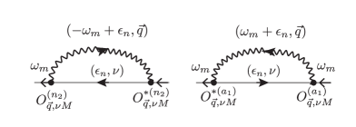
Figure 3: Additions Feynman diagrams for normal contributions to the self-energy of the $\alpha$-mode at finite temperatures. Solid lines correspond to gapped fermionic excitations in the wire and wavy lines to bosinic excitations in the molecular condensate.

The calculation of the Matsubara Green’s function is very similar to that of the Green’s function at zero temperature and based on the Dyson equation

$$G_{TM}^{-1}(i\varepsilon_{n})=G_{TM}^{(0)-1}(i\varepsilon_{n})-\Sigma_{TM}(i\varepsilon_{n})=i\varepsilon_{n}-E_{M}-\Sigma_{TM}(i\varepsilon_{n})$$

with the Matsubara self-energy $\Sigma_{TM}(i\varepsilon_{n})$ and $G_{TM}^{(0)}(i\varepsilon_{n})=(i\varepsilon_{n}-E_{M})^{-1}$. The lowest (second-order) contribution to the self-energy are shown in Fig. 1 (with real frequencies replaced by Matsubara ones) and Fig. 3 where the solid and dashed lines corresponds to $G_{T\nu}^{(0)}(i\varepsilon_{n})=(i\varepsilon_{n}-E_{\nu})^{-1}$ and $D_{T\mathbf{q}}^{(0)}(i\omega_{m})=(i\omega_{m}-\epsilon_{q}+i0)^{-1}$, respectively. (Note that, similar to the $T=0$ case, the ”anomalous” contributions can be ignored.) After performing the summation over the (bosonic) Matsubara frequency $\omega_{m}=2\pi Tm$, we obtain

$$\Sigma_{TM}(i\varepsilon_{n})=\Sigma_{TM}^{(1)}(i\varepsilon_{n})+\Sigma_{TM}^{(2)}(i\varepsilon_{n}),$$

where

$$\Sigma_{TM}^{(1)}(i\varepsilon_{n}) =\sum_{\mathbf{q},\nu}\left[\frac{\left|O_{\mathbf{q}\nu M}^{(n1)}\right|^{2}}{i\varepsilon_{n}-(E_{\nu}+\epsilon_{q})}+\frac{4\left|O_{\mathbf{q}\nu M}^{(a2)}\right|^{2}}{i\varepsilon_{n}+E_{\nu}+\epsilon_{q}}\right]$$

$$\times\left[1+n_{B}(\epsilon_{q})-n_{F}(E_{\nu})\right]$$

and

$$\Sigma_{TM}^{(2)}(i\varepsilon_{n}) =\sum_{\mathbf{q},\nu}\left[\frac{\left|O_{\mathbf{q}\nu M}^{(n2)}\right|^{2}}{i\varepsilon_{n}-(E_{\nu}-\epsilon_{q})}+\frac{4\left|O_{\mathbf{q}\nu M}^{(a1)}\right|^{2}}{i\varepsilon_{n}+E_{\nu}-\epsilon_{q}}\right]$$

$$\times\left[n_{B}(\epsilon_{q})+n_{F}(E_{\nu})\right]$$

with $n_{F\nu}(T)$ and $n_{B\mathbf{q}}(T)$ being the fermionic and bosonic occupation numbers of the gapped modes $\alpha_{v}$ and excitations $b_{\mathbf{q}}$ in the condensate, respectively. With the analytic continuation $i\varepsilon_{n}\rightarrow\varepsilon+i0$, an approximate solution of the equation $G_{M}^{R}(\varepsilon)^{-1}=\varepsilon-E_{M}-\Sigma_{TM}(\varepsilon+i0)=0$ for the pole of the Green’s function reads

$$\varepsilon_{M\ast}\approx E_{M}+\Sigma_{TM}(E_{M}+i0)=E_{M}+\delta_{T}E_{M}-i\gamma_{M},$$

where

$$\Sigma_{TM}(E_{M}+i0) =\Sigma_{TM}^{(1)}(E_{M}+i0)+\Sigma_{TM}^{(2)}(E_{M}+i0)$$

$$=\sum_{\mathbf{q},\nu}\left[\frac{4\left|O_{\mathbf{q}\nu M}^{(a2)}\right|^{2}}{E_{\nu}+\epsilon_{q}+E_{M}}-\frac{\left|O_{\mathbf{q}\nu M}^{(n1)}\right|^{2}}{E_{\nu}+\epsilon_{q}-E_{M}}\right][1+n_{B}(\epsilon_{q})-n_{F}(E_{\nu})]$$

$$+\sum_{\mathbf{q},\nu}\left[\frac{4\left|O_{\mathbf{q}\nu M}^{(a1)}\right|^{2}}{E_{\nu}-\epsilon_{q}+E_{M}+i0}-\frac{\left|O_{\mathbf{q}\nu M}^{(n2)}\right|^{2}}{E_{\nu}-\epsilon_{q}-E_{M}-i0}\right][n_{B}(\epsilon_{q})+n_{F}(E_{\nu})]$$

$$=\delta_{T}E_{M}-i/\tau_{M}$$

provides the correction $\delta_{T}E_{M}=\mathrm{\text{Re}}\Sigma_{TM}(E_{M}+i0)$ to the energy of the mode $\alpha_{M}$, as well as its inverse life-time $\tau_{M}^{-1}=-\mathrm{\text{Im}}\Sigma_{TM}(E_{M}+i0)$. Note that the first term $\Sigma_{TM}^{(1)}(E_{M})$ which generalizes Eq. (45) to finite temperatures, contributes to $\delta_{T}E_{M}$ only because the energy denominators are never zero (for this reason we skipped the $i0$ there), while the second term $\Sigma_{TM}^{(2)}(E_{M}+i0)$ which is non-zero only at finite temperatures, contributes to both $\delta_{T}E_{M}$ and $\tau_{M}^{-1}$.

By using Eqs. (38) and (39) for the matrix elements $O_{\mathbf{q}\nu M}^{(n1)}$ and $O_{\mathbf{q}\nu M}^{(a2)}$, the terms $\Sigma_{TM}^{(1)}(E_{M})$ and can be written in the form

$$\Sigma_{TM}^{(1)}(E_{M})\approx\sum_{\mathbf{q},\nu}\left[\frac{4\text{Re}(\left\langle 0\left|H_{R}^{(+)}{}^{{\dagger}}\right|\mathbf{q}\nu\right\rangle\left\langle\mathbf{q}\nu\left|H_{L}^{(+)}\right|0\right\rangle)}{E_{\nu}+\epsilon_{q}}-2E_{M}\frac{\left|\left\langle\mathbf{q}\nu\left|H_{L}^{(+)}\right|0\right\rangle\right|^{2}+\left|\left\langle\mathbf{q}\nu\left|H_{R}^{(+)}\right|0\right\rangle\right|^{2}}{(E_{\nu}+\epsilon_{q})^{2}}\right][1+n_{B}(\epsilon_{q})-n_{F}(E_{\nu})]$$ (58)

which recovers Eqs. (40) and (41) for $T=0$. The term $\Sigma_{TM}^{(2)}(E_{M})$ can also be written in the form involving matrix elements of the operators $H_{L,R}^{(+)}$, if one notices [see Eqs. (36) and (32)] that

$$O_{\mathbf{q}\nu M}^{(n2)}=\left\langle\nu\left|H_{L}^{(+)}+H_{R}^{(+)}\right|\mathbf{q}\right\rangle$$

and

$$2O_{\mathbf{q}\nu M}^{(a1)}=\left\langle\nu\left|H_{L}^{(+)}-H_{R}^{(+)}\right|\mathbf{q}\right\rangle.$$

The corresponding expression reads

$$\Sigma_{TM}^{(2)}(E_{M}+i0) =\sum_{\mathbf{q},\nu}\left\{2\text{Re}(\left\langle\mathbf{q}\left|H_{R}^{(+)}{}^{{\dagger}}\right|\nu\right\rangle\left\langle\nu\left|H_{L}^{(+)}\right|\mathbf{q}\right\rangle)\left[\frac{1}{E_{\nu}-\epsilon_{q}+E_{M}+i0}+\frac{1}{E_{\nu}-\epsilon_{q}-E_{M}-i0}\right]\right.$$

$$\left.+(\left|\left\langle\nu\left|H_{L}^{(+)}\right|\mathbf{q}\right\rangle\right|^{2}+\left|\left\langle\nu\left|H_{R}^{(+)}\right|\mathbf{q}\right\rangle\right|^{2})\left[\frac{1}{E_{\nu}-\epsilon_{q}+E_{M}+i0}-\frac{1}{E_{\nu}-\epsilon_{q}-E_{M}-i0}\right]\right\}$$

$$\times[n_{B}(\epsilon_{q})+n_{F}(E_{\nu})]$$

and contains again two different types of correlations: long-range correlations between the edges (the first line) and short-range correlations at the edges (the second line). The real part of $\Sigma_{TM}^{(2)}(E_{M}+i0)$ contains terms with the correlations of the both types:

$$\mathrm{\text{Re}}\Sigma_{TM}^{(2)}(E_{M}+i0) \approx\mathrm{p.V.}\sum_{\mathbf{q},\nu}\frac{4\text{Re}(\left\langle\mathbf{q}\left|H_{R}^{(+)}{}^{{\dagger}}\right|\nu\right\rangle\left\langle\nu\left|H_{L}^{(+)}\right|\mathbf{q}\right\rangle)}{E_{\nu}-\epsilon_{q}}[n_{B}(\epsilon_{q})+n_{F}(E_{\nu})]$$

$$+2E_{M}\left\{\frac{\partial}{\partial E_{M}}\mathrm{p.V.}\sum_{\mathbf{q},\nu}\frac{\left|\left\langle\nu\left|H_{L}^{(+)}\right|\mathbf{q}\right\rangle\right|^{2}+\left|\left\langle\nu\left|H_{R}^{(+)}\right|\mathbf{q}\right\rangle\right|^{2}}{E_{\nu}-\epsilon_{q}+E_{M}}[n_{B}(\epsilon_{q})+n_{F}(E_{\nu})]\right\}_{E_{M}=0},$$ (59)

while the dominant contribution to the imaginary part of $\Sigma_{TM}^{(2)}(E_{M}+i0)$ and, therefore, to the life-time $\tau_{M}$, comes from the short-range correlations:

$$\tau_{M}^{-1}=-\mathrm{\text{Im}}\Sigma_{TM}(E_{M}+i0)\approx 2\pi\sum_{\mathbf{q},\nu}(\left|\left\langle\nu\left|H_{L}^{(+)}\right|\mathbf{q}\right\rangle\right|^{2}+\left|\left\langle\nu\left|H_{R}^{(+)}\right|\mathbf{q}\right\rangle\right|^{2})[n_{B}(\epsilon_{q})+n_{F}(E_{\nu})]\delta(E_{\nu}-\epsilon_{q}),$$ (60)

where we have neglected terms which are exponentially small in the system size $L$.

It follows from Eqs. (58) and (59) that the correction to the energy $\delta_{T}E_{M}$ and, therefore, the energy itself, remains exponentially small with the system size $L$, even at finite temperatures $T\ll\Delta_{m}$. The leading temperature correction to the zero-temperature result (56) comes from the low-energy bosonic excitations with $\epsilon_{q}\lesssim T\ll E_{\nu}\leq\Delta_{m}$ [the number of fermionic excitations $n_{F}(E_{\nu})$ is exponentially small at such temperatures, $n_{F}(E_{\nu})\lesssim\exp(-\Delta_{m}/T)\ll 1$, and can be neglected]. These bosonic excitations are phonons with $q\ll\xi_{BEC}^{-1}$, for which, as it follows from Eqs. (33), (34), and (35), one has

$$\left\langle\nu\left|H_{L(R)}^{(+)}\right|\mathbf{q}\right\rangle=-\left\langle\mathbf{q}\nu\left|H_{L(R)}^{(+)}\right|0\right\rangle,$$ (61)

and the leading temperature correction $\delta_{T}E_{M}$ reads

$$\delta_{T}E_{M} \approx 4\sum_{\mathbf{q},\nu}\left[\frac{2\text{Re}(\left\langle 0\left|H_{R}^{(+)}{}^{{\dagger}}\right|\mathbf{q}\nu\right\rangle\left\langle\mathbf{q}\nu\left|H_{L}^{(+)}\right|0\right\rangle)}{E_{\nu}}-E_{M}\frac{\left|\left\langle\mathbf{q}\nu\left|H_{L}^{(+)}\right|0\right\rangle\right|^{2}+\left|\left\langle\mathbf{q}\nu\left|H_{R}^{(+)}\right|0\right\rangle\right|^{2}}{E_{\nu}^{2}}\right]n_{B}(\varepsilon_{q})$$

$$\equiv\delta_{T}E_{M}^{(1)}+\delta_{T}E_{M}^{(2)},$$

where, similar to the $T=0$ case, we introduce the two contributions $\delta_{T}E_{M}^{(1)}$ and $\delta_{T}E_{M}^{(2)}$ which contain long-range and short-range correlations, respectively.

The calculation of the dominant (for large $L$) term $\delta_{T}E_{M}^{(1)}$ can be performed in the same way as for the case of zero temperature. With the expressions (47) and (48) for the matrix elements, the energy correction $\delta_{T}E_{M}^{(1)}$ reads

$$\delta_{T}E_{M}^{(1)} \approx 8K_{0}^{2}\int\frac{d\mathbf{q}}{(2\pi)^{3}}n_{B}(\varepsilon_{q})\int_{-\pi/a}^{\pi/a}\frac{adk}{2\pi}\frac{f_{q}^{2}(u_{k}+v_{k})^{2}\sin^{2}ka}{E_{k}}\sum_{j_{1},j_{2}}f_{Lj_{1}}f_{Rj_{2}}e^{i(q_{x}+k)(j_{1}-j_{2})a}$$

$$=8K_{0}^{2}\sum_{j_{1},j_{2}}f_{Lj_{1}}f_{Rj_{2}}\int\frac{d\mathbf{q}}{(2\pi)^{3}}f_{q}^{2}n_{B}(\varepsilon_{q})e^{iq_{x}(j_{1}-j_{2})a}\int_{-\pi/a}^{\pi/a}\frac{adk}{2\pi}\frac{(u_{k}+v_{k})^{2}\sin^{2}ka}{E_{k}}e^{ik(j_{1}-j_{2})a}$$

$$=8K_{0}^{2}\sum_{j_{1},j_{2}}f_{Lj_{1}}f_{Rj_{2}}C_{B}(j_{1}-j_{2})h(j_{1}-j_{2}).$$ (62)

We see that in this approximation, the correlation function of the pair of excitations decouples into the product of bosonic

$$C_{B}(j_{1}-j_{2})=\int\frac{d\mathbf{q}}{(2\pi)^{3}}f_{q}^{2}n_{B}(\varepsilon_{q})e^{iq_{x}(j_{1}-j_{2})a}$$ (63)

and fermionic

$$h(j_{1}-j_{2})=\int_{-\pi/a}^{\pi/a}\frac{adk}{2\pi}\frac{(u_{k}+v_{k})^{2}\sin^{2}ka}{E_{k}}e^{ik(j_{1}-j_{2})a}$$ (64)

correlation functions, respectively. The function $h(j_{1}-j_{2})$ is calculated in Appendix B, Eqs. (143) and (144), and is nonzero only for $\left|j_{1}-j_{2}\right|\sim l_{M}/a\sim 1$. The bosonic correlation function $C_{B}(j_{1}-j_{2})$ can be represented in the form

$$C_{B}(j_{1}-j_{2}) =\frac{1}{4\pi^{2}}\frac{mT}{\hbar^{2}}\frac{1}{\left|j_{1}-j_{2}\right|a}\int_{0}^{\infty}dx\frac{\sin[\frac{T\left|j_{1}-j_{2}\right|a}{\hbar c}x]}{e^{x}-1}$$

$$=\frac{\pi}{2}-\frac{\hbar c}{2T\left|j_{1}-j_{2}\right|a}+\frac{\pi}{\exp(2\pi T\left|j_{1}-j_{2}\right|a/\hbar c)-1}.$$

For $\left|j_{1}-j_{2}\right|\sim l_{M}/a\sim 1$, one has $T\left|j_{1}-j_{2}\right|a/\hbar c\sim\left|j_{1}-j_{2}\right|(T/J)(Ja/\hbar c)\sim\left|j_{1}-j_{2}\right|(T/\Delta_{m})\lambda\ll 1$, and for such values of $\left|j_{1}-j_{2}\right|$ the correlation function takes the simple form

$$C_{B}(j_{1}-j_{2})\approx\frac{1}{24}\frac{mT^{2}}{\hbar^{3}c},$$

where the power is determined by the space volume of phonons ($\sim T^{3}$) and by the square of the matrix elements ($\sim q^{-1}\rightarrow T^{-1}$). (Note that this expression for the bosonic correlation function is valid for distances $r\ll\hbar c/T\sim a(J/T)\lambda^{-1}\gg a$.)

For $\delta_{T}E_{M}^{(1)}$ we now have

$$\delta_{T}E_{M}^{(1)} =\frac{1}{3}\frac{mT^{2}K_{0}^{2}}{\hbar^{3}c}\sum_{j_{1},j_{2}}f_{Lj_{1}}f_{Rj_{2}}h(j_{1}-j_{2})$$

$$\approx-\frac{1}{3}\frac{mT^{2}K_{0}^{2}}{\hbar^{3}c}2\left|A\right|^{2}\sum_{j_{1},j_{2}}\rho^{L+1+j_{1}-j_{2}}\cos[(L+1+j_{1}-j_{2})\theta]h(j_{1}-j_{2})$$

$$=-\frac{1}{3}\frac{mT^{2}K_{0}^{2}}{\hbar^{3}c}2\left|A\right|^{2}L\rho^{L+1}\left\{h(0)\cos[(L+1)\theta]+\sum_{s>0}\rho^{s}h(s)\cos[(L+1+s)\theta]+\rho^{-1}h(-1)\cos(L\theta)\right\},$$

where we use Eq. (53) and keep only the dominant term for large $L$. It follows from the results of Appendix B that the leading contribution for small $\rho$ comes from the last term, and we finally get

$$\delta_{T}E_{M} \approx\delta_{T}E_{M}^{(1)}\approx\frac{1}{3}\frac{mT^{2}K_{0}^{2}}{\hbar^{3}c}2\left|A\right|^{2}\frac{1}{4J(1+\alpha)}L\rho^{L}\cos(L\theta)$$ (65)

$$=\frac{1}{6}\frac{mT^{2}K_{0}^{2}}{\hbar^{3}c}\frac{\Delta(4J^{2}-\mu^{2})}{J(4J^{2}-4\Delta^{2}-\mu^{2})}\frac{1}{J+\Delta}L\rho^{L}\cos(L\theta)$$

$$\sim\frac{\Delta^{2}}{E_{R}}\frac{1}{n_{M}a^{3}}\left(\frac{T}{J}\right)^{2}\lambda Le^{-La/l_{M}}\sim E_{M}\frac{\Delta}{E_{R}}\left(\frac{T}{J}\right)^{2}\lambda L\sim\delta E_{M}\left(\frac{T}{J}\right)^{2}\lambda.$$

We see that in the considered temperatures $T\ll\Delta_{m}\sim J$, the correction to the energy $E_{M}$ of the Majorana mode due to thermal fluctuations is much smaller than that due to quantum fluctuations, and can be neglected.

The life-time $\tau_{M}$, Eq. (60), is determined by the correlations at the edges and, hence, does not depend on the length of the wire $L$. On the other hand, the dependence of $\tau_{M}$ on temperature is exponential, $\tau_{M}\sim\exp(\Delta_{m}/T)$, as a result of exponentially small number of thermal excitations, both bosonic and fermionic, with energies larger than the gap $\Delta_{m}$ in the wire, $n_{B}(\varepsilon_{q})$,$\,n_{F}(E_{\nu})\approx\exp(-\Delta_{m}/T)$ for $E_{\nu},\,\epsilon_{q}\gtrsim\Delta_{m}$ and $T\ll\Delta_{m}$. Note that relevant bosonic excitations must also have energies larger than $\Delta_{m}$ because of the energy conservation condition in Eq. (60). The reason for this is the conservation of the parity: The change in the population of the mode $\alpha_{M}$ has to be accompanied by the change in the population of one of the gapped mode $\alpha_{\nu}$. For this to happen, one needs either a bosonic excitation with the energy larger than $\Delta_{m}$ which excites a gapped fermionic mode (terms $\alpha_{M}\alpha_{\nu}^{{\dagger}}b_{\mathbf{q}}$ or $\alpha_{M}^{{\dagger}}\alpha_{\nu}^{{\dagger}}b_{\mathbf{q}}$ in the Hamiltonian), or a gapped fermionic excitation which is annihilated with emission of a bosonic excitation ($\alpha_{M}\alpha_{\nu}b_{\mathbf{q}}^{{\dagger}}$ or $\alpha_{M}^{{\dagger}}\alpha_{\nu}b_{\mathbf{q}}^{{\dagger}}$ terms). In both cases, the probability to find such excitation is of the order of $\exp(-\Delta_{m}/T)$.

We now calculate $\tau_{M}$ for temperatures $T\ll\Delta_{m}$. In this case, the relevant bosonic excitations have energies $\varepsilon_{q}=E_{\nu}\gtrsim\Delta_{m}\sim J\ll\hbar c\xi_{\text{BEC}}^{-1}$, and are, therefore, phonons with wave vectors $q\sim J/\hbar c\sim\lambda a^{-1}\ll a^{-1}$. This allows us to use Eqs. (61), (47), and (48) for the matrix elements in Eq. (60) with the result (the contributions from the right and left edges are identical)

$$\tau_{M}^{-1} =4\pi K_{0}^{2}\sum_{j_{1},j_{2}}f_{Lj_{1}}f_{Lj_{2}}\int\frac{d\mathbf{q}}{(2\pi)^{3}}f_{q}^{2}\int_{-\pi/a}^{\pi/a}\frac{adk}{2\pi}\sin^{2}(ka)e^{i(q_{x}+k)a(j_{1}-j_{2})}[n_{B}(\epsilon_{q})+n_{F}(E_{k})]\delta(E_{k}-\epsilon_{q})$$

$$\approx 8\pi K_{0}^{2}\sum_{j_{1},j_{2}}f_{Lj_{1}}f_{Lj_{2}}\int_{-\pi/a}^{\pi/a}\frac{adk}{2\pi}\sin^{2}(ka)e^{-E_{k}/T}e^{ika(j_{1}-j_{2})}\int\frac{d\mathbf{q}}{(2\pi)^{3}}f_{q}^{2}\delta(E_{k}-\epsilon_{q})e^{iq_{x}a(j_{1}-j_{2})},$$

where we take into account that $n_{F}(E_{k})\approx n_{B}(\epsilon_{q})\approx\exp(-E_{k}/T)$ for $E_{k}=\epsilon_{q}\gtrsim\Delta_{m}\gg T$. The result of the integration over $\mathbf{q}$ is

$$\int\frac{d\mathbf{q}}{(2\pi)^{3}}f_{q}^{2}\delta(E_{k}-\epsilon_{q})e^{iq_{x}a(j_{1}-j_{2})}=\frac{m}{4\pi^{2}\hbar^{3}}\frac{\sin[E_{k}a(j_{1}-j_{2})/\hbar c]}{a(j_{1}-j_{2})},$$

and, if we take into account that $E_{k}a\left|j_{1}-j_{2}\right|/\hbar c\sim\lambda\left|j_{1}-j_{2}\right|\ll 1$ for $\left|j_{1}-j_{2}\right|\lesssim l_{M}/a\sim 1$, the expression for $\tau_{M}^{-1}$ can be written in the form

$$\tau_{M}^{-1}=\frac{2mK_{0}^{2}}{4\pi\hbar^{4}c}\sum_{j_{1},j_{2}}f_{Lj_{1}}f_{Lj_{2}}\int_{-\pi/a}^{\pi/a}\frac{adk}{2\pi}\sin^{2}(ka)E_{k}e^{-E_{k}/T}e^{ika(j_{1}-j_{2})}.$$

We next perform the summation over $j_{1}$ and $j_{2}$:

$$\sum_{j_{1},j_{2}}f_{Lj_{1}}f_{Lj_{2}}e^{ika(j_{1}-j_{2})}=\left|\sum_{j}f_{Lj}e^{ikaj}\right|^{2}\approx\frac{1-\beta^{2}}{(E_{k}/2J)^{2}},$$

where we use Eq. (20) for $f_{Lj}$, and obtain

$$\tau_{M}^{-1}=\frac{8mJ^{2}K_{0}^{2}(1-\beta^{2})}{\pi\hbar^{4}c}\int_{-\pi/a}^{\pi/a}\frac{adk}{2\pi}\frac{\sin^{2}(ka)}{E_{k}}e^{-E_{k}/T}.$$ (66)

The final integral over $k$ can be calculated analytically in two limiting cases when the temperature $T$, being much smaller than the gap $\Delta_{m}$, is much smaller (i) or much larger (ii) than the band-width of fermionic excitations $\Delta E_{b}\approx 2J(1-\alpha+\left|\beta\right|)$ (the latter case can be realized when the band of fermionic excitations is narrow, $\Delta E_{b}\ll J$, which happens for $1-\alpha^{2}\ll 1$ and $\left|\beta\right|\ll$ $1-\alpha^{2}$).

In the first case, $T\ll\Delta E_{b}$, the main contribution comes from the vicinities of two minima of $E_{k}$ at $k=\pm k_{F}=\pm a^{-1}\arccos[-\beta/(1-\alpha^{2})]$ inside the Brillouin zone $-\pi/a\leq k\leq\pi/a$. Near these minima, $E_{k}$ can be approximated as

$$E_{k}\approx\Delta_{m}+J\alpha^{-1}\frac{(1-\alpha^{2})^{2}-\beta^{2}}{\sqrt{(1-\alpha^{2}-\beta^{2})(1-\alpha^{2})}}\delta k_{\pm}^{2},$$

where $\delta k_{\pm}=k\mp k_{F}$, and, after extending the integration over $\delta k_{\pm}$ to infinite limits, we obtain

$$\tau_{M}^{-1}\approx\frac{4mJ^{2}K_{0}^{2}}{\pi\hbar^{4}c\Delta_{m}}e^{-\Delta_{m}/T}(1-\beta^{2})\sqrt{\frac{2}{\pi}\frac{T\Delta_{m}}{J^{2}}\frac{(1-\alpha^{2})^{2}-\beta^{2}}{(1-\alpha^{2})^{3}}}.$$ (67)

The life-time $\tau_{M}$ estimated from this expression,

$$\tau_{M}\sim\frac{\hbar}{J}\frac{E_{R}}{J\lambda}\sqrt{\frac{J}{T}}e^{\Delta_{m}/T}\gg\frac{\hbar}{J},$$ (68)

contains not only the exponential factor $\exp(\Delta_{m}/T)$ but also large prefactor ($E_{R}/J\lambda)\sqrt{J/T}\gg 1$, altogether making $\tau_{M}$ much larger than the characteristic time $\hbar/J$ in the wire.

In the second case, $\Delta E_{b}\ll T\ll\Delta_{m}$, we can set $E_{k}\approx\Delta_{m}$ in Eq. (66) and obtain

$$\tau_{M}^{-1}\approx\frac{4mJ^{2}K_{0}^{2}}{\pi\hbar^{4}c\Delta_{m}}e^{-\Delta_{m}/T}(1-\beta^{2}).$$ (69)

An estimate of the life-time $\tau_{M}$ in this case,

$$\tau_{M}\sim\frac{\hbar}{J}\frac{E_{R}}{J\lambda}e^{\Delta_{m}/T}\gg\frac{\hbar}{J},$$ (70)

also shows exponential dependence on temperature with the large temperature-independent prefactor $E_{R}/J\lambda\gg 1$, such that also in this case $\tau_{M}$ is much larger than the characteristic time $\hbar/J$ in the wire.

The life-time $\tau_{M}$ provides an estimate for the thermalization time of the mode $\alpha_{M}$ and, therefore, for the “relaxation”time of Majorana correlations – the time during which the correlations evolve from their initial values to the stationary ones. If, for example, we the mode $\alpha_{M}$ is unpopulated initially (i.e., $-i\left\langle\gamma_{L}\gamma_{R}\right\rangle=1$), than its occupation $n_{M}(t)=\left\langle\alpha_{M}^{{\dagger}}(t)\alpha_{M}(t)\right\rangle$ and the related Majorana correlation $-i\left\langle\gamma_{L}(t)\gamma_{R}(t)\right\rangle$ for times $t>\tau_{M}$ can be estimated as

$$1-2n_{M}(t)=-i\left\langle\gamma_{L}(t)\gamma_{R}(t)\right\rangle\sim\exp[-2L\exp(-\Delta_{m}/T)].$$ (71)

This estimate is based on purely statistical arguments with an account of the parity constraint ($L$ in the exponent corresponds to the number of the gapped modes in the systems). Without this constraint, the mode $\alpha_{M}$ will be effectively at infinite temperature with $n_{M}(t)-1/2\sim\exp(-E_{M}/T)\approx 0$ for any realistic temperature $T$. Eq. (71) shows that no correlations between Majorana fermions survive at finite temperature in the thermodynamic limit $L\rightarrow\infty$. On the other hand, in a mesoscopic system, the thermal degradation of the initial correlations can still be sufficiently small, allowing quantum operations with Majorana fermions for times $t>\tau_{M}$ with acceptable fidelity.

VIII Concluding remarks

Our results show the prospect for creation and manipulation of Majorana fermions in ultra-cold system of atoms and molecules. For a Kitaev’s topological wire which can be realized by coupling fermionic atoms in an optical lattice to a superfluid molecular reservoir, we have shown that the coupling between Majorana edge states in the wire and the corresponding splitting in the ground state degeneracy decay exponentially with the length of the wire. This results also holds at finite temperatures lower than the gap $\Delta_{m}$ of the bulk fermionic excitations in the wire. With the possibility of having the localization length of the Majorana edge states to be of the order of few lattice spacings, this ensures that already relatively short wires with $L\gtrsim 10$ are sufficient for creation of well-separated Majorana edge states, their detection as “zero-energy”edge states via, for example, spectroscopic measurements LiangJiang ; Nascimbene ; MajAtom3 , and demonstration their non-Abelian character via braiding MajAtom5 ; MajAtom6 .

Thermal fluctuations however result in the decay of the correlations between the Majorana edge states on a time scale $\tau_{M}$ to the values which decreases exponentially with the length of the wire $L$. This limits quantum operations with Majorana fermions to times less than $\tau_{M}$. Note, however, that under the rather general conditions of our implementation scheme, see Appendix A, one has $E_{R}/J\lambda\gtrsim 10^{3}$ and, already for $\Delta_{m}/T=3$, the life-time $\tau_{M}$ estimated from Eq. (70) is five orders of magnitude larger than $\hbar/\Delta_{m}$.This is sufficient for the implementation of the brading protocol and simple quantum computation algorithms, see Refs. MajAtom5 and MajAtom6 , based on adiabatic manipulations of Majorana edge states in atomic wires.

To perform quantum operations during longer times, $t>\tau_{M}$, one can consider systems of mesoscopic wires with the length which is chosen to obtain the highest fidelity in a given experimental setup. This optimal length is a result of the competition between Eq. (71) which favours smaller $L$ in order to minimize the destructive effects of thermal fluctuations on Majorana correlations, and Eqs. (23), (56), and (65) which suggest larger $L$ to minimize the energy of the Majorana mode $E_{M}$ which determines the splitting of the ground state. $E_{M}$ therefore sets the low bound on the speed of adiabatic manipulations with Majorana states and, hence, on their error. As an illustration of what one could expect, we consider the wire of the length $L=10$ with the localization length of the Majorana edge states $l_{M}=3a$. From Eq. (71) we then find that thermal fluctuations reduce the Majorana correlations to $\approx 70\%$ of their values when $\Delta_{m}/T=4$, and to $\approx 90\%$ when $\Delta_{m}/T=5$. At the same time, Eq. (56) gives $E_{M}\sim 10^{-2}\Delta_{m}$, such that we can find the speed $t_{A}^{-1}$, $\hbar/\Delta_{m}\ll t_{A}\ll\hbar/E_{M}$, at which operations with Majorana fermions are adiabatic with respect to the gap $\Delta_{m}$ and diabatic with respect to the splitting $E_{M}$. The latter allows us to consider the ground-state manifold as being degenerate during the operations – the condition when non-Abelian statistics of Majorana fermions determines the result of operations with them. Based on the above estimates we can conclude that adiabatic quantum manipulations with Majorana fermions in systems of ultracold atoms and molecules are not unrealistic.

IX Acknowledgement

We would like to thank P. Zoller for raising our interest to the problem and for many stimulating discussions during the work. We also acknowledge useful discussions with M. Dalmonte, S. Diehl, C. Kraus, A. Kamenev, S. Nascimbène, H. Pichler, T. Ramos, E. Rico, and C. Salomon. This project was supported by the ERC Synergy Grant UQUAM and the SFB FoQuS (FWF Project No. F4016-N23). Y. H. acknowledges the support from the Institut für Quanteninformation GmbH.

Appendix A Microscopic Model

Here we describe a realization of the Kitaev Hamiltonian using fermionic atoms in an optical lattice coupled to a superfluid reservoir through Raman lasers. We shall first illustrate our microscopic model for a setup in which the reservoir is a molecular BEC, and derive the effective Hamiltonian (1) in the main text. Later, we will extend to more general cases where the superfluid reservoir consists of fermion pairs in the BEC-BCS crossover regime.

A.1 Setup and microscopic Hamiltonian

We consider fermionic atoms in three internal states, labeled as $\mid\uparrow\rangle$, $\mid\downarrow\rangle$ and $|3\rangle$, having energies $\varepsilon_{\uparrow}$, $\varepsilon_{\downarrow}$, and $\varepsilon_{3}$, respectively. Atoms in the state $|3\rangle$ can be trapped in a strongly anisotropic optical lattice where tunneling is only allowed in one direction, leading to the realization of a quasi-$1D$ fermionic quantum gas (wire). Atoms in the internal states $\mid\uparrow\rangle$ and $\mid\downarrow\rangle$ can form a Feshbach molecule. The molecules are cooled to form a molecular BEC at sufficiently low temperature, which acts as a reservoir for pairs of atoms in the lattice.

For the atoms in the wire, the corresponding field operator $\hat{\chi}_{3}(\mathbf{r})$ can be expanded on the basis of Wannier functions as

$$\hat{\chi}_{3}(\mathbf{r})=\sum_{j}w(\mathbf{r}-\mathbf{r}_{j})\hat{a}_{j},$$ (72)

where $\hat{a}_{j}$ is the annihilation operator for an atom at the lattice site $\mathbf{r}_{j}=ja\mathbf{e}_{x}+y_{0}\mathbf{e}_{y}+z_{0}\mathbf{e}_{z}$ with $a$ being the spatial period in the $x$-direction, and we assume a Gaussian form for the Wannier function (in the lowest band tight binding approximation)

$$w(\mathbf{r})=\frac{1}{\pi^{\frac{3}{4}}\sigma_{x}^{\frac{1}{2}}\sigma_{\perp}}e^{-x^{2}/2\sigma_{x}^{2}-(y^{2}+z^{2})/2\sigma_{\perp}^{2}},$$ (73)

with $\sigma_{x}$ and $\sigma_{\perp}$ being the extension of the Wannier function $w(\mathbf{r})$ in the $x$- and transverse directions, respectively, which satisfy the condition $\sigma_{\perp}\ll\sigma_{x}\ll a$. The Hamiltonian for atoms hopping freely in the wire therefore reads

$$H_{\mathrm{L}}=\sum_{j}[-J_{0}(\hat{a}_{j}^{{\dagger}}\hat{a}_{j+1}+\hat{a}_{j+1}^{\dagger}\hat{a}_{j})-\varepsilon_{3}^{\prime}\hat{a}_{j}^{{\dagger}}\hat{a}_{j}],$$ (74)

where $\epsilon_{3}^{\prime}=\epsilon_{3}-\varepsilon_{\mathrm{lat}}$ is the chemical potential of a bare atom trapped in each well in the lattice and, and as usual, we limit ourselves to the nearest-neighbor hopping $J_{0}$.

For the atoms in the internal state $|\sigma\rangle$ in the bulk reservoir (with volume $V$), the corresponding field operator $\hat{\chi}_{\sigma}(\mathbf{r})$ can be written in terms of ’plane waves’ as

$$\hat{\chi}_{\sigma}(\mathbf{r})=\frac{1}{\sqrt{V}}\sum_{\mathbf{p}}\hat{c}_{\mathbf{p}\sigma}e^{i\mathbf{p}\cdot\mathbf{r}},$$ (75)

where $\hat{c}_{\mathbf{p}\sigma}$ is the annihilation operator for an atom in the internal state $|\sigma\rangle$ with momentum $\mathbf{p}$. Two atoms in the internal states $\mid\uparrow\rangle$ and $\mid\downarrow\rangle$, respectively, can form a Feshbach molecule. A Feshbach molecule of a size $a_{s}$ (or the scattering length between $\mid\uparrow\rangle$ and $\mid\downarrow\rangle$ atoms) has an energy $\epsilon_{\text{mol}}=\epsilon_{\uparrow}+\epsilon_{\downarrow}-E_{b}$ ($E_{b}=\hbar^{2}/ma_{s}^{2}$ is the binding energy). The corresponding molecular field operator $\hat{\phi}^{{\dagger}}(\mathbf{r})$ is expressed as $\hat{\phi}^{{\dagger}}(\mathbf{r})=\frac{1}{\sqrt{V}}\sum_{\mathbf{q}}e^{-i\mathbf{q}\cdot\mathbf{r}}\hat{b}_{\mathbf{q}}^{{\dagger}}$, where the molecular operator $\hat{b}_{\mathbf{q}}^{{\dagger}}$ can be written in terms of the atomic operator $\hat{c}_{\mathbf{p}\sigma}^{{\dagger}}$ as

$$\hat{b}_{\mathbf{q}}^{{\dagger}}=\sum_{\mathbf{k}}\varphi_{\mathbf{k}}\hat{c}_{\mathbf{q}/2+\mathbf{k},\uparrow}^{{\dagger}}\hat{c}_{\mathbf{q}/2-\mathbf{k},\downarrow}^{{\dagger}},$$ (76)

with $\varphi_{k}$ being the molecular wave function (in the momentum space)

$$\varphi_{\mathbf{k}}=\left(\frac{8\pi}{a_{s}}\right)^{1/2}\frac{1}{k^{2}+1/a_{s}^{2}}.$$

When the molecules are sufficiently cooled to form a molecular condensate, the corresponding Hamiltonian reads, (for simplicity we assume that molecules do not feel the optical lattice potential)

$${H}_{\mathrm{BEC}}=\int d\mathbf{r}\hat{\phi}^{{\dagger}}\left(-\frac{\hbar^{2}}{2m}\nabla^{2}-\mu_{\text{M}}+\frac{g_{\text{M}}}{2}\hat{\phi}^{{\dagger}}\hat{\phi}\right)\hat{\phi},$$

where $m=2m_{a}$ is the mass of the molecule, $g_{\text{M}}=4\pi\hbar^{2}a_{\text{M}}/m$ is the coupling constant with $a_{\text{M}}\approx 0.6a_{s}$ PetrovSolomonSchlyapnikov being the molecule-molecule scattering length, and $\mu_{\text{M}}$ is the chemical potential of molecules in the condensate. Hereafter, we will assume weak interaction regime $n_{\text{M}}a_{\text{M}}^{3}<1$, where $n_{\text{M}}$ is the density of molecules.

The coupling between the atoms in the wire and the molecules in the reservoir is introduced via a set of Raman transitions between the atomic internal state $|3\rangle$ and the states $|\sigma\rangle$, described by the Hamiltonian (after the rotating-wave approximation)

$$H_{\mathrm{R}}=\sum_{\sigma=\uparrow,\downarrow}\int d\mathbf{r}\Omega_{\sigma}[e^{(i\mathbf{k}_{\sigma}\mathbf{r}-i\omega_{\sigma}t)}\hat{\chi}_{\mathrm{L}}^{{\dagger}}(\mathbf{r})\hat{\chi}_{\sigma}(\mathbf{r})+\text{h.c.}],$$ (77)

where $\Omega_{\sigma}$ is the Rabi frequency, while $\omega_{\sigma}$ and $\mathbf{k}_{\sigma}$ are the frequency and momentum of the Raman laser, respectively. A crucial condition in Eq. (77) is to have $\mathbf{k}_{\uparrow}\neq\mathbf{k}_{\downarrow}$ for the reasons that will soon become clear. By using Eqs. (72) and (75), we rewrite Hamiltonian (77) as

$$H_{\text{R}}=\frac{1}{\sqrt{V}}\sum_{\mathbf{p},j,\sigma}[\Omega_{\sigma}e^{i(\mathbf{p}+\mathbf{k}_{\sigma})\cdot\mathbf{r}_{j}-i\omega_{\sigma}t}M^{*}_{\mathbf{p}+\mathbf{k}_{\sigma}}\hat{a}^{{\dagger}}_{j}\hat{c}_{\mathbf{p}\sigma}+\text{h.c.}],$$ (78)

with

$$M_{\mathbf{p}+\mathbf{k}_{\sigma}}=\int d\mathbf{r}_{1}w(\mathbf{r}_{1})e^{-i(\mathbf{p}+\mathbf{k}_{\sigma})\cdot\mathbf{r}_{1}},$$ (79)

being the Fourier transformation of the Wannier function $w(\mathbf{r})$.

Overall, the total Hamiltonian for an atomic wire coupled to a molecular reservoir via Raman beams can be written as

$${H}={H}_{\mathrm{L}}+{H}_{\mathrm{BEC}}+{H}_{\mathrm{int}}+{H}_{\mathrm{R}},$$ (80)

where the Hamiltonian $H_{\mathrm{int}}$ describes the short-range interaction between atoms in the lattice and molecules in the BEC, reading

$${H}_{\mathrm{int}} =g_{a\text{M}}\int d\mathbf{r}\hat{\chi}_{\mathrm{L}}^{{\dagger}}(\mathbf{r})\hat{\chi}_{\mathrm{L}}(\mathbf{r})\hat{\phi}^{{\dagger}}(\mathbf{r})\hat{\phi}(\mathbf{r})$$

$$\approx\sum_{j}\int d\mathbf{r}g_{j}(\mathbf{r})\hat{a}_{j}^{{\dagger}}\hat{a}_{j}\hat{\phi}^{{\dagger}}(\mathbf{r})\hat{\phi}(\mathbf{r}),$$ (81)

with $g_{a\text{M}}$ being the corresponding coupling constant (the corresponding scattering length  $a_{a\text{M}}\approx 1.2a_{s}$, see PetrovSolomonSchlyapnikov ; PetrovSolomonSchlyapnikov1 ) and $g_{j}(\mathbf{r})=g_{a\text{M}}w(\mathbf{r}-\mathbf{r}_{j})^{2}$. As we shall show below, the crucial ingredient in the Hamiltonian (1) consists in the Raman transitions between the atomic internal states ($H_{\mathrm{R}}$), which provide a mechanism to inducing the $p$-wave pairing term in the wire out of the $s$-wave superfluid reservoir.

A.2 Raman-induced conversion of molecules into pairs of atoms

Now, we will show in detail the realization of the conversion of a molecule in the reservoir to a pair of atoms in the lattice described by the Hamiltonian

$$H_{\mathrm{conv}}=\sum_{j,j^{\prime}}\int d\mathbf{r[}K_{jj^{\prime}}(\mathbf{r})\hat{a}_{j}^{{\dagger}}\hat{a}_{j^{\prime}}^{{\dagger}}\hat{\phi}(\mathbf{r})+\mathrm{H.c.}]$$ (82)

from the setup described by Eq. (80). The physics behind the pair transfer via Raman processes can be described as follows (see Fig. 4).

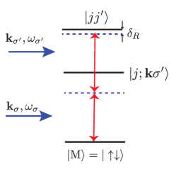
Figure 4: (Color online) A schematic illustration of the mechanism converting a molecule from the condensate into a pair of atoms in the optical lattice via two successive off-resonant Raman transitions. The first Raman transition changes the internal state of a constituent atom in the molecule ($|\text{M}\rangle=|\uparrow\downarrow\rangle$), from $\mid\downarrow(\uparrow)\rangle$ to $|3\rangle$. As a result, the molecule is broken into one atom trapped in the lattice site $j$ and one unpaired $\mid\uparrow(\downarrow)\rangle$ atom with momenta $\mathbf{k}$. This unpaired atom is transferred into the lattice after the second Raman transition, which changes its internal state from $\mid\uparrow(\downarrow)\rangle$ to $|3\rangle$. The overall process of transferring a molecule $|\text{M}\rangle$ in the reservoir into a pair of atoms in the lattice $|jj^{\prime}\rangle$ via absorbing two Raman photons is nearly resonant, with a small two-photon detunning $\delta_{R}$ determined by the resonant condition in Eq. (84).

The action of $H_{\text{R}}$ on a molecule, according to Eq. (76), flips the internal state of one of the constituent atom from $|\sigma\rangle\rightarrow|3\rangle$, thereby generating processes where a molecule breaks into an atom in the internal state $|3\rangle$ and an atom in the internal state $|\sigma\rangle$, in particular, the process where the generated $|3\rangle$ atom is trapped in the lattice. The Hamiltonian describing the transfer of a molecule into an atom in the wire and a unpaired atom in the internal state $|\sigma\rangle$ moving in the reservoir (and vice versa) reads

$$\!\!\!\!H_{\text{R}}^{\text{M}}=\!\!\frac{1}{\sqrt{V}}\!\!\sum_{\mathbf{k},j}\!\Big{[}\Omega_{\uparrow}\!e^{-i\omega_{\uparrow}t}e^{i(\frac{\mathbf{q}}{2}\!+\!\mathbf{k}\!+\!\mathbf{k}_{\uparrow})\cdot\mathbf{r}_{j}}M_{\frac{\mathbf{q}}{2}\!+\!\mathbf{k}\!+\!\mathbf{k}_{\uparrow}}^{\ast}\varphi_{\mathbf{k}}\hat{a}_{j}^{{\dagger}}\hat{c}_{\frac{\mathbf{q}}{2}\!-\!\mathbf{k}\downarrow}^{{\dagger}}\hat{b}_{\mathbf{q}}\!-\!\Omega_{\downarrow}e^{-i\omega_{\downarrow}t}e^{i(\frac{\mathbf{q}}{2}-\mathbf{k}+\mathbf{k}_{\downarrow})\cdot\mathbf{r}_{j}}M_{\frac{\mathbf{q}}{2}\!-\!\mathbf{k}\!+\!\mathbf{k}_{\downarrow}}^{\ast}\varphi_{\mathbf{k}}\hat{a}_{j}^{{\dagger}}\hat{c}_{\frac{\mathbf{q}}{2}\!+\!\mathbf{k}\uparrow}^{{\dagger}}\hat{b}_{\mathbf{q}}\!+\!\text{h.c.}\Big{]}.$$ (83)

Then, in the second Raman process, the unpaired $|\sigma\rangle$ atom in the reservoir can be further transferred into the internal state $|3\rangle$ and trapped in the lattice. Overall, after two successive Raman processes, a transfer of a molecule in the reservoir into a pair of atoms in the wire is achieved, corresponding to $\hat{b}^{{\dagger}}\rightarrow\hat{a}_{j}^{{\dagger}}\hat{c}_{\mathbf{p}\sigma}^{{\dagger}}\rightarrow\hat{a}_{j}^{{\dagger}}\hat{a}_{j^{\prime}}^{{\dagger}}$, and vice versa.

Let us state the main conditions under which the two continuous Raman processes lead to a resonant transfer of a molecule from the BEC into a pair of atoms in the optical lattice (and vice versa), but keeping the transfer of a single atom from the reservoir to the lattice off-resonant. To this end, let us first briefly summarize the hierarchy of relevant energy levels. A Feshbach molecule with a size $a_{s}$ in the BEC has an energy $\epsilon_{\text{mol}}+\epsilon_{\text{MM}}$, where $\epsilon_{\text{MM}}=g_{\text{M}}n_{\text{M}}$ describes the interaction between molecules in the BEC ($g_{\text{a{M}}}=3\pi\hbar^{2}a_{\text{a{M}}}/m$ with $a_{\text{M}}\approx 0.6a_{s}$ and $m$ being the mass of an atom). On the other hand, the average energy of a pair of atoms in a wire can be written as $2(\epsilon_{3}^{\prime}-\frac{1}{2}\delta_{\text{R}}+\epsilon_{\text{aM}})$, where $\delta_{\text{R}}$ is the two-photon detuning (see Fig. 4) and $\epsilon_{\text{aM}}=g_{\text{aM}}n_{\text{M}}$ is the mean-field interaction between an atom in the wire and surrounding molecules. (For simplicity, we have assumed that the atom-molecule interaction is independent of the internal state of an atom, and thereby consider $g_{\text{aM}}=3\pi\hbar^{2}a_{\text{aM}}/m$ with $a_{\text{aM}}\approx 1.2a_{s}$ being the atom-molecule scattering length.) As a result, a nearly resonant transfer between a molecule in the BEC and a pair of atoms in the wire is achieved when the two Raman photons provide an energy satisfying the energy conservation reading

$$\hbar\omega_{\uparrow}+\hbar\omega_{\downarrow}=2(\epsilon_{3}-\frac{\delta_{\text{R}}}{2}+\epsilon_{\text{aM}})-(\epsilon_{\text{ mol}}+\epsilon_{\text{MM}}),$$ (84)

where $\delta_{\text{R}}$ is a small detuning associated with the two-photon Raman processes. In terms of $\delta_{\sigma}=\hbar\omega_{\sigma}+\epsilon_{\sigma}-(\epsilon_{3}^{\prime}-\frac{1}{2}\delta_{\text{R}})$ defined in the main text and assuming $\delta_{\uparrow}\approx\delta_{\downarrow}$, the resonance condition in Eq. (84) can be recast as $\delta_{\sigma}=\delta_{0}$ with

$$\delta_{0}=\epsilon_{\text{aM}}+\frac{1}{2}E_{b}-\frac{1}{2}\epsilon_{\text{MM}}.$$ (85)

Meanwhile, note that the energy cost for breaking a molecule into an atom in the wire and an atom moving in the reservoir is

$$\Delta E_{\sigma} =[\epsilon_{3}^{\prime}+(\epsilon_{\sigma}+\epsilon_{\mathbf{p}}^{0})+2\epsilon_{\text{aM}}]-[{\epsilon}_{\text{mol}}+\epsilon_{\text{MM}}-\hbar\omega_{\sigma}]$$

$$=\epsilon_{\mathbf{p}}^{0}+\delta_{0},$$ (86)

where $\epsilon_{\mathbf{p}}^{0}$ is the kinetic energy of an unpaired atom in the reservoir. Under the resonance condition in Eq. (85), it is obvious that $\Delta E_{\sigma}\neq 0$, and therefore, the state in which an atom is generated in the wire and an atom remains unpaired in the BEC is energetically prohibited, and serves as an intermediate state for the ultimate realization of pair transfer.

Now, we are readily to derive the amplitude $K_{jj^{\prime}}(\mathbf{r})$ in Eq. (82) for converting a molecule in the reservoir (labeled by the state $|\text{M}\rangle$ ) into a pair of atoms at site $j$ and $j^{\prime}$ in the wire (labeled by the state $|jj^{\prime}\rangle$). By straightforwardly applying the second-order perturbation theory, together with Eqs. (85) and (86), we obtain

$$K_{jj^{\prime}}(\mathbf{q})=-\sum_{k,\sigma}\frac{\langle jj^{\prime}|H_{\text{R}}|\mathbf{k}\sigma;j^{\prime}\rangle\langle\mathbf{k}\sigma;j^{\prime}|H^{\text{M}}_{\text{R}}|\text{M}\rangle}{\epsilon_{\mathbf{k}}^{0}+\delta_{0}}.$$ (87)

Substituting Eqs. (78) and (83) into Eq. (87), we find

$$K_{jj^{\prime}}(\mathbf{q})=-\frac{16i}{V}\Omega\sin\left(\frac{\mathbf{k}_{d}\mathbf{r}_{jj^{\prime}}}{2}\right)e^{i(\mathbf{q}+\mathbf{k}_{c})\cdot\mathbf{R}_{jj^{\prime}}}M_{c}^{*}\left(\mathbf{q}+\mathbf{k}_{c}\right)\times\frac{1}{a_{s}^{2}}\sum_{\mathbf{k}}\frac{\varphi_{k}e^{-\tilde{k}_{x}^{2}\sigma_{x}^{2}-\tilde{k}_{\perp}^{2}\sigma_{\perp}^{2}}e^{i\mathbf{k}\cdot\mathbf{r}_{jj^{\prime}}}}{k^{2}+1/l_{0}^{2}}.$$ (88)

with

$$l^{2}_{0}=\frac{\hbar^{2}}{2m\delta_{0}}.$$ (89)

In Eq. (88), $\Omega=\Omega_{\uparrow}\Omega_{\downarrow}/E_{b}$ is the effective Rabi frequency for pair transfer, $\mathbf{k}_{d}=\mathbf{k}_{\uparrow}-\mathbf{k}_{\downarrow}$, $\mathbf{k}_{c}=\mathbf{k}_{\uparrow}+\mathbf{k}_{\downarrow}$, $\mathbf{R}_{jj^{\prime}}=(\mathbf{r}_{j}+\mathbf{r}_{j^{\prime}})/2=\frac{(j+j^{\prime})a}{2}\mathbf{e}_{x}+y_{0}\mathbf{e}_{y}+z_{0}\mathbf{e}_{z}$, and $\mathbf{r}_{jj^{\prime}}=\mathbf{r}_{j}-\mathbf{r}_{j^{\prime}}=(j-j^{\prime})a\mathbf{e}_{x}$, $M_{c}^{*}(\mathbf{q})=\exp[q_{x}^{2}\sigma_{x}^{2}/4-(q_{y}^{2}+q_{z}^{2})\sigma_{\perp}^{2}/4]$, $\tilde{\mathbf{k}}=\mathbf{k}+\mathbf{k}_{d}/2$ and $\tilde{k}_{\perp}^{2}=\tilde{k}_{y}^{2}+\tilde{k}_{z}^{2}$. Note that for a molecule of a size $a_{s}\sim a$, the dominant contribution to the sum in Eq. (88) comes from $k\sim 1/a_{s}$, and therefore under the condition $\sigma_{\perp}\ll\sigma_{x}\ll a$ imposed previously, one has $k\sigma_{x(\perp)}\ll 1$. Also taking into account $\mathbf{k}_{d}\sim 1/a$, we can thus simplify Eq. (88) by approximating $\exp[-\sigma_{x(\perp)}^{2}\tilde{k}_{x(\perp)}^{2}]\approx 1$. Consequently, after transforming back to the real space using $K_{jj^{\prime}}(\mathbf{r})=\int K_{jj^{\prime}}(\mathbf{q})e^{-i\mathbf{q}\cdot\mathbf{r}}d\mathbf{q}$, we obtain the amplitude $K_{jj^{\prime}}(\mathbf{r})$ in the Hamiltonian (82) as

$$K_{jj^{\prime}}(\mathbf{r})=i\Omega F(\mathbf{r}-\mathbf{R}_{jj^{\prime}})e^{i\mathbf{k}_{c}\cdot\mathbf{R}_{jj^{\prime}}}\sin\left(\frac{\mathbf{k}_{d}\mathbf{r}_{jj^{\prime}}}{2}\right)\frac{2a_{s}}{|\mathbf{r}_{jj^{\prime}}|}\frac{e^{-|\mathbf{r}_{jj^{\prime}}|/l_{0}}-e^{-|\mathbf{r}_{jj^{\prime}}|/a_{s}}}{1-a_{s}^{2}/l_{0}^{2}}.$$ (90)

with $F(\mathbf{r})=8\sqrt{2/\pi a_{s}^{3}}e^{-x^{2}/\sigma_{x}^{2}-(y^{2}+z^{2})/\sigma_{\perp}^{2}}$. In the weak interaction regime $[n_{\text{M}}a_{s}^{3}\ll 1]$ under consideration,

$$a_{s}/l_{0}\approx 1+3\pi n_{\text{M}}a_{s}^{3}.$$ (91)

Thus to the leading order of $n_{\text{M}}a_{s}^{3}$, we obtain

$$K_{jj^{\prime}}(\mathbf{r})=i\Omega\sin(\frac{\mathbf{k}_{d}\mathbf{r}_{jj^{\prime}}}{2})F(\mathbf{r}-\mathbf{R}_{jj^{\prime}})e^{i\mathbf{k}_{c}\cdot\mathbf{R}_{jj^{\prime}}-|r_{jj^{\prime}}|/a_{s}},$$ (92)

where $\Omega=\Omega_{\uparrow}\Omega_{\downarrow}/E_{b}$ is the effective Rabi frequency for pair transfer, $F\left(\mathbf{r}\right)=8\sqrt{2/\pi a_{s}^{3}}\exp[-x^{2}/\sigma_{x}^{2}-(y^{2}+z^{2})/\sigma_{\perp}^{2}]$, $\mathbf{k}_{d}=\mathbf{k}_{\uparrow}-\mathbf{k}_{\downarrow}$, $\mathbf{k}_{c}=\mathbf{k}_{\uparrow}+\mathbf{k}_{\downarrow}$, $\mathbf{R}_{jj^{\prime}}=(\mathbf{r}_{j}+\mathbf{r}_{j^{\prime}})/2=\frac{(j+j^{\prime})a}{2}\mathbf{e}_{x}+y_{0}\mathbf{e}_{y}+z_{0}\mathbf{e}_{z}$, and $\mathbf{r}_{jj^{\prime}}=\mathbf{r}_{j}-\mathbf{r}_{j^{\prime}}=(j-j^{\prime})a\mathbf{e}_{x}$.

Equation (92) shows that, in order to engineer a $p$-wave pairing, the condition $\mathbf{k}_{\uparrow}\neq\mathbf{k}_{\downarrow}$ must be fulfilled, such that the amplitude $K_{jj^{\prime}}$ is antisymmetric, $K_{jj^{\prime}}=-K_{j^{\prime}j}$. In addition, $K_{jj^{\prime}}$ is in general complex: $K_{jj^{\prime}}=|K_{jj^{\prime}}|e^{i\theta_{jj^{\prime}}}$ with $\theta_{jj^{\prime}}=\frac{\pi}{2}+\mathbf{k}_{c}\mathbf{R}_{jj^{\prime}}$. We can, however engineer a homogeneous phase $\theta_{jj^{\prime}}$ along the $x$-direction (direction of the lattice) by choosing $\mathbf{k}_{c}$,  say, along the $y$-axis, $\mathbf{k}_{c}=k_{c}\mathbf{e}_{y}$, such that $\theta_{jj^{\prime}}=\frac{\pi}{2}+k_{c}y_{0}$ depends only on the wire position in $y$-direction. Taking into account the exponential fall-off $K_{jj^{\prime}}\sim e^{-|r_{jj^{\prime}}|/a_{s}}$ and $a_{s}\sim a$, we will consider $K_{jj^{\prime}}$ to be nonzero only for the nearest-neighbor sites $\left|j-j^{\prime}\right|=1$ with $K_{j,j+1}=K_{j}$.

A.3 Raman-induced hopping

Apart from inducing the pair transfer, the Raman processes also contribute to the correction to the hopping term in Eq. (74) via the reservoir-mediated intermediated processes, corresponding to a Hamiltonian

$$H_{\mathrm{J}}=\sum_{j,j^{\prime}}\delta J_{jj^{\prime}}\hat{a}_{j}^{{\dagger}}\hat{a}_{j^{\prime}}+\text{h.c.}.$$

As will be seen below, there are two processes (labeled as process $a$ and process $b$, respectively) that contribute to $\delta J_{jj^{\prime}}$ (see Fig. 5):

$$\delta J_{jj^{\prime}}=\delta J_{jj^{\prime}}^{a}+\delta J_{jj^{\prime}}^{b},$$ (93)

where the process $a$ involves only single-atom states, while the process $b$ also involves molecules in the reservoir. In what follows, we derive the hopping amplitude $\delta J_{jj^{\prime}}^{a(b)}$ in detail, respectively.

(i) In the process $a$ (see Fig. 5(a)),

Figure 5: (Color online) Two Raman-induced processes contributing to the correction in the hopping amplitude $\delta J_{jj^{\prime}}$. In the process (a), an optically trapped atom at the lattice site $j$ hops to the lattice site $j^{\prime}$ via an intermediate single-atom process, in which the atom changes its internal state to $|\sigma\rangle$ and untrapped from the lattice (and vice versa) under the Raman drive. (b) describes a molecule-mediated hopping, where the intermediate process involves breaking of a molecule $|\text{M}\rangle$ into an atom on the lattice site and an unpaired $|\sigma^{\prime}\rangle$ atom with momenta $\mathbf{k}$, and vice versa.

an atom in the wire, say, at the lattice site $\mathbf{r}_{j^{\prime}}$ labeled as $|j^{\prime}\rangle$, when acted under the Hamiltonian $H_{\text{R}}$, flips its internal state from $|3\rangle$ to $|\sigma\rangle$ and transfers into a unpaired atom moving in the BEC, labeled as $|\mathbf{k}\sigma\rangle$. Such single-atom transfer costs an energy

$$\Delta E^{(a)}=\epsilon_{\sigma}+\epsilon_{\mathbf{k}}^{0}+\hbar\omega_{\sigma}-\epsilon_{3}^{\prime}=\epsilon_{\mathbf{k}}^{0}+\delta_{0}\neq 0,$$

and is thereby off-resonant. Then, via the second Raman transition $H_{\text{R}}$, the atom in the state $|\mathbf{k}\sigma\rangle$ can be transferred back into an atom in the wire, but at position $\mathbf{r}_{j}$, labeled as $|j\rangle$. Overall, one realizes a process $\hat{a}_{j}^{{\dagger}}a_{j^{\prime}}$ (and vice versa) with the second-order hopping amplitude given by

$$\delta J_{jj^{\prime}}^{(a)}=-\sum_{\sigma}\sum_{\mathbf{k}}\frac{\langle j|H_{\text{R}}|\mathbf{k}\sigma\rangle\langle\mathbf{k}\sigma|H_{\text{R}}|{j^{\prime}}\rangle}{\epsilon_{k}^{0}+\delta_{0}}.$$ (94)

The matrix element in Eq. (94) can be straightforwardly evaluated with Eq. (78), and after some calculation, we obtain

$$\delta J_{jj^{\prime}}^{(a)}=-\frac{16\pi^{3/2}\Omega_{J}}{a_{s}^{2}}\frac{\sigma_{x}\sigma_{\perp}^{2}}{V}\sum_{\mathbf{k}}\frac{e^{-\sigma_{x}^{2}\tilde{k}_{x}^{2}-\sigma_{\perp}^{2}\tilde{k}_{\perp}^{2}+i(\mathbf{k}+\mathbf{k}_{c})\cdot\mathbf{r}_{jj^{\prime}}}}{k^{2}+1/l_{0}^{2}},$$ (95)

with

$$\Omega_{J}=\frac{\Omega_{\uparrow}^{2}e^{i\mathbf{k}_{d}\mathbf{r}_{jj^{\prime}}/2}+\Omega_{\downarrow}^{2}e^{-i\mathbf{k}_{d}\mathbf{r}_{jj^{\prime}}/2}}{E_{b}}.$$

Having in mind $\tilde{k}_{x(\perp)}\sigma_{x(\perp)}\ll 1$ under the condition $\sigma_{\perp}\ll\sigma_{x}\ll a$, we evaluate Eq. (95 ) as

$$\delta J_{jj^{\prime}}^{(a)}=-\Omega_{J}\frac{4\pi^{1/2}\sigma_{x}\sigma_{\perp}^{2}}{a_{s}^{3}}\frac{e^{-|\mathbf{r}_{jj^{\prime}}|/l_{0}}}{|\mathbf{r}_{jj^{\prime}}|/a_{s}}e^{i\frac{\mathbf{k}_{c}}{2}\cdot\mathbf{r}_{jj^{\prime}}}.$$ (96)

For weak interaction ($n_{\text{M}}a_{s}^{3}\ll 1$), we submit the expansion (91) into Eq. (96), and obtain in the first order in $n_{\text{M}}a_{s}^{3}$ (we set $\mathbf{k}_{c}=y_{0}\mathbf{e}_{y}$ such that $\mathbf{k}_{c}\cdot\mathbf{r}_{jj^{\prime}}=0$ as in the main text)

$$\delta J_{jj^{\prime}}^{(a)} =-\Omega_{J}\frac{4\pi^{1/2}\sigma_{x}\sigma_{\perp}^{2}}{a_{s}^{3}}\frac{e^{-|\mathbf{r}_{jj^{\prime}}|/a_{s}}}{|\mathbf{r}_{jj^{\prime}}|/a_{s}}$$

$$\times(1-\frac{|\mathbf{r}_{jj^{\prime}}|}{a_{s}}3\pi n_{M}a_{s}^{3}).$$ (97)

It follows from Eq. (97) that $|\mathbf{r}_{jj^{\prime}}|\sim a_{s}$ because of the exponential decay $\exp(-|\mathbf{r}_{jj^{\prime}}|/a_{s})$, and as a result, the contribution $\frac{|\mathbf{r}_{jj^{\prime}}|}{a_{s}}n_{\text{M}}a_{s}^{3}\ll 1$.

(ii) The process $b$ (see Fig. 5 (b)) involves simultaneously an atom at lattice site $\mathbf{r}_{j^{\prime}}$ and a molecule in the BEC, labeled as $|j^{\prime};\text{M}\rangle$. The action of $H_{\text{R}}^{\text{M}}$ on the state $|j^{\prime};\text{M}\rangle$ leads to an intermediate state where two atoms are in the wire and one unpaired atom moves in the BEC, labeled as $|jj^{\prime};\mathbf{p}\sigma\rangle$, with an energy cost given by

$$\Delta E^{(b)} =[2\epsilon_{3}^{\prime}+\epsilon_{\sigma}+\epsilon_{\mathbf{p}}^{0}+2\epsilon_{\text{aM}}]-[\epsilon_{3}^{\prime}+\epsilon_{\text{mol}}+\epsilon_{\text{MM}}+\hbar\omega_{\sigma^{\prime}}]$$

$$=\epsilon_{\mathbf{p}}^{0}+\delta_{0}.$$ (98)

Then, the action of $H_{\text{R}}^{\text{M}}$ on the intermediate state $|jj^{\prime};\mathbf{p}\sigma\rangle$ generates a process where a molecule is created in the BEC and an atom remains at the lattice site $\mathbf{r}_{j}$ in the wire, labeled as $|j;\text{M}\rangle$. The overall amplitude between the initial state $|j^{\prime};\text{M}\rangle$ and the final state $|j;\text{M}\rangle$ is given by

$$\delta J_{jj^{\prime}}^{(b)}=\sum_{\mathbf{k}}\frac{\langle j;{\text{M}}|H^{\text{M}}_{\text{R}}|jj^{\prime};\mathbf{p}\sigma\rangle\langle jj^{\prime};\mathbf{p}\sigma|H^{\text{M}}_{\text{R}}|j^{\prime};{\text{M}}\rangle}{\epsilon_{k}^{0}+\delta_{0}}.$$ (99)

It follows from Eq. (83) that the matrix element of $H^{\text{M}}_{\text{R}}$ between the intermediate state $|jj^{\prime};\mathbf{p}\sigma\rangle$ and the state $|j^{\prime};{\text{M}}\rangle$ is derived as

$$\langle\mathbf{p}\uparrow;jj^{\prime}|H^{\text{M}}_{\text{R}}|j^{\prime};\text{M}\rangle =-\frac{\Omega_{\downarrow}}{\sqrt{V}}M^{*}_{\mathbf{p}+\mathbf{k}_{\downarrow}}e^{i(\mathbf{p}+\mathbf{k}_{\downarrow})\cdot\mathbf{r}_{j^{\prime}}}\varphi_{\mathbf{k}}\sqrt{n_{\text{M}}}\delta_{\mathbf{p},\frac{\mathbf{q}}{2}-\mathbf{k}},$$

$$\langle\mathbf{p}\downarrow;jj^{\prime}|H^{\text{M}}_{\text{R}}|j^{\prime};\text{M}\rangle =\frac{\Omega_{\uparrow}}{V}M^{*}_{\mathbf{p}+\mathbf{k}_{\uparrow}}e^{i(\mathbf{p}+\mathbf{k}_{\downarrow})\cdot\mathbf{r}_{j^{\prime}}}\varphi_{\mathbf{k}}\sqrt{n_{\text{M}}}\delta_{\mathbf{p},\frac{\mathbf{q}}{2}+\mathbf{k}},$$ (100)

where $n_{\text{M}}$ is the condensate density of molecular BEC. Substituting Eq. (100) into Eq. (99), and after straightforward calculation, we obtain (to the first order of $n_{\text{M}}a_{s}^{3}\ll 1$),

$$\delta J_{jj^{\prime}}^{(b)}\approx\Omega_{J}\left(\pi n_{\text{M}}a_{s}^{3}\right)\frac{4\sqrt{\pi}\sigma_{x}\sigma_{\perp}^{2}}{a_{s}^{3}}e^{-\frac{|\mathbf{r}_{jj^{\prime}}|}{a_{s}}}\left(1+\frac{|\mathbf{r}_{jj^{\prime}}|}{a_{s}}\right).$$ (101)

Consequently, combination of Eqs. (96) and (101) yields (in the limit $n_{\text{M}}a_{s}^{3}\ll 1$)

$$\delta J_{jj^{\prime}}=(4\sqrt{\pi})(\sigma_{x}\sigma_{\perp}^{2}/a_{s}^{3})e^{i\mathbf{k}_{c}\mathbf{r}_{jj^{\prime}}/2}\Omega_{J}\frac{e^{-|\mathbf{r}_{jj^{\prime}}|/a_{s}}}{|\mathbf{r}_{jj^{\prime}}|/a_{s}}\left[1-\pi n_{\text{M}}a_{s}^{3}\frac{|\mathbf{r}_{jj^{\prime}}|}{a_{s}}\left(4+\frac{|\mathbf{r}_{jj^{\prime}}|}{a_{s}}\right)\right].$$ (102)

Note that by tuning $\mathbf{k}_{c}=k_{c}\mathbf{e}_{y}$, the phase factor $\exp(i\mathbf{k}_{c}\mathbf{r}_{jj^{\prime}}/2)$ in Eq. (102) vanishes, and $\delta J_{jj^{\prime}}$ can be made real by choosing $\Omega_{1}=\Omega_{2}$. Similar to the pair transfer amplitude, $\delta J_{jj^{\prime}}$ also decays exponentially with increasing $\left|j-j^{\prime}\right|$, and therefore, we will take into account only the nearest-neighbor contribution $\delta J_{jj+1}$. As a result, the nearest-neighbour hopping amplitude $J_{0}$ in Eq. (3) will be renormalized to

$$J=J_{0}+\delta J_{j,j+1}.$$ (103)

Collecting above results, it is clear that after elimination of the Raman processes, we arrive at the effective Hamiltonian (1) in the main text for the setup. There, the renormalized chemical potential for a fermionic atom in the wire is given by $\mu_{0}=\epsilon_{3}^{\prime}-\delta_{\text{R}}/2$.

A.4 Reservoir in the regime of BEC-BCS crossover

In above derivations, we note that when $n_{\text{M}}a_{s}^{3}$ approaches unity, $n_{\text{M}}a_{s}^{3}<1$, the intermediate processes involving molecules in the BEC plays increasingly important role compared to single-particle process, and previous expansions in terms of $n_{M}a_{s}^{3}$ are no longer valid. In order to evaluate the Raman-induced pairing amplitude $K_{j,j^{\prime}}(\mathbf{r})$ and hopping amplitude $\delta J_{j,j^{\prime}}$ in this case, we use the theory of BCS-BEC crossover Ketterle08 , which corresponds to considering a reservoir in the molecular side of the BCS-BEC crossover regime.

We begin with writing the particle operator $\hat{c}_{\mathbf{k}\sigma}$ introduced in Eq. (75) in terms of the Bogoliubov quasi-particle operators $\hat{\gamma}_{\mathbf{k}\sigma}$:

$$\hat{\gamma}_{\mathbf{k}\uparrow} =u_{\mathbf{k}}\hat{c}_{\mathbf{k}\uparrow}-\upsilon_{\mathbf{k}}\hat{c}_{-\mathbf{k}\downarrow}^{{\dagger}},$$

$$\hat{\gamma}_{-\mathbf{k}\downarrow}^{{\dagger}} =u_{\mathbf{k}}\hat{c}_{-\mathbf{k}\downarrow}^{{\dagger}}+\upsilon_{\mathbf{k}}\hat{c}_{\mathbf{k}\uparrow}^{{\dagger}},$$ (104)

where $u_{\mathbf{k}}$ and $\upsilon_{\mathbf{k}}$ are the standard wave functions of the Bogoliubov quasi-particles, and $E_{k}$ is the corresponding excitation energy given by

$$E_{k}=\sqrt{\Delta_{b}^{2}+(\epsilon_{k}^{0}-\mu_{b})^{2}},$$

where $\epsilon_{\mathbf{k}}^{0}$ is the kinetic energy of a free atom, while $\mu_{b}$ and $\Delta_{b}$ are the chemical potential and the gap of the superconducting reservoir, respectively. In the BCS-BEC crossover regime, both $\mu_{b}$ and $\Delta_{b}$ are self-consistently determined from the gap equation and the number equation (see Ref. Ketterle08 for expressions and the derivations). While subsequent derivations apply to the whole crossover regime, for our purpose, here we will limit ourselves to the molecular side of the crossover.

Substituting Eqs. (104) into Eqs. (78) and (83), and using, as before, the second-order perturbation theory, we obtain the paring amplitude

$$K_{jj^{\prime}}\left(\mathbf{r}\right)=-16i\Omega\sin\left(\frac{\mathbf{k}_{d}\cdot\mathbf{r}_{jj^{\prime}}}{2}\right)F\left(\mathbf{r}\!-\mathbf{R}_{jj^{\prime}}\right)e^{i\mathbf{k}_{c}\cdot\mathbf{R}_{jj^{\prime}}}\frac{E_{b}}{2V}\sum_{k}\frac{\Delta_{\text{b}}}{E_{k}^{2}}e^{i\mathbf{k}\cdot\mathbf{r}_{jj^{\prime}}},$$ (105)

and the hopping amplitude

$$\delta J_{jj^{\prime}}=\Omega_{J}\left(8\pi^{3/2}\sigma_{x}\sigma_{\perp}^{2}\right)\frac{E_{b}}{V}\sum_{\mathbf{k}}\frac{\epsilon_{\mathbf{k}}^{0}-\mu_{b}}{E_{k}^{2}}e^{i\mathbf{k}\cdot\mathbf{r}_{jj^{\prime}}}.$$ (106)

After performing the summations in $\mathbf{k}$ in Eqs. (105) and ( 106), respectively, we arrive at

$$K_{jj^{\prime}}\left(\mathbf{r}\right) =i\frac{4\Omega}{\pi}\sin\left(\frac{\mathbf{k}_{d}\mathbf{r}_{jj^{\prime}}}{2}\right)\frac{M\left(\frac{|\mathbf{r}_{jj^{\prime}}|}{a_{s}}\right)}{\sqrt{n_{\text{M}}a_{s}^{3}}}F\left(\mathbf{r}-\mathbf{R}_{jj^{\prime}}\right)e^{i\mathbf{k}_{c}\cdot\mathbf{R}_{jj^{\prime}}},$$ (107)

$$\delta J_{jj^{\prime}} =4\pi^{1/2}\Omega_{\text{J}}\frac{\sigma_{x}\sigma_{\perp}^{2}}{a_{s}^{3}}Q\left(\frac{|\mathbf{r}_{jj^{\prime}}|}{a_{s}}\right),$$ (108)

where we have introduced the functions

$$M(d)=\frac{e^{-d\sqrt{\rho}\sin\frac{\theta}{2}}}{d}\sin\left[d\sqrt{\rho}\cos\frac{\theta}{2}\right],$$

$$Q(d)=\frac{e^{-d\sqrt{\rho}\sin\frac{\theta}{2}}}{d}\cos\left[d\sqrt{\rho}\cos\frac{\theta}{2}\right],$$

with

$$\rho=\frac{\sqrt{\mid\mu_{b}\mid^{2}+\mid{\Delta}_{b}\mid^{2}}}{E_{F}};$$

$$\sin^{2}\left(\frac{\theta}{2}\right)=\frac{1}{2}\left[1-\frac{\mu_{b}}{\sqrt{\mid\mu_{b}\mid^{2}+\mid{\Delta}_{b}\mid^{2}}}\right];$$

$$\cos^{2}\left(\frac{\theta}{2}\right)=\frac{1}{2}\left[1+\frac{\mu_{b}}{\sqrt{\mid\mu_{b}\mid^{2}+\mid{\Delta}_{b}\mid^{2}}}\right].$$

Here, $E_{F}={\hbar^{2}(6\pi^{2}n_{\text{M}})^{2/3}}/{2m}$ is the Fermi energy of the reservoir.

A.5 Optimal conditions for Majorana edge states

We now look for the optimal conditions, under which (1) the overlap between the two Majorana edge modes are minimized, i.e. the Majoranas modes ares strongly localized at the edges; (2) the gap in the bulk spectrum is as large as possible. This can be achieved by tuning $J\sim|\Delta|$ and $\mu_{f}\sim 0$ in Eq. (8) in the main text (here we drop the subscript in $\Delta_{\phi_{0}}$ for clarity), corresponding to the realization of a nearly ideal Kitaev chain. The chemical potential $\mu_{f}\approx 0$ can be realized via a fine control of the two-photon detuning $\delta_{R}$, as described earlier. On the other hand, the hopping amplitude $J$ [see Eqs. ( 103) and (108)] and pairing amplitude $|\Delta|$ [see Eqs. (9) and (107) ] depend on characteristic parameters for the reservoir (e.g. molecular size $a_{s}$, density $n_{M}$) and for the wire (e.g. lattice depth $V_{x}$, lattice constant $a$). In order to find the optimal ratio $a/a_{s}$ between the lattice constant $a$ and the molecule size $a_{s}$, we scan $|\Delta|$ and $J$ as a function of $a/a_{s}$ while fixing other parameters in Eqs. (107) and (108), as illustrated in Fig. 6. There, for typical parameters $\sigma_{x}\sigma_{\perp}^{2}/a^{3}=0.03$ and $n_{\text{M}}a_{s}^{3}=0.01$, we find a maximum gap arising at $a_{s}\sim a/3$. Then, we fix the molecular size at $a_{s}=a/3$, and scan $|\Delta|$ and $J$ as a function of the lattice depth $V_{x}$, respectively, as shown in Fig. 7. We see that the condition $J\sim|\Delta|$ can be achieved for $V_{x}\sim 10E_{r}$ with $E_{r}=\hbar^{2}/2m\lambda^{2}$ denoting the recoil energy, which is well in reach in current experiment facilities.

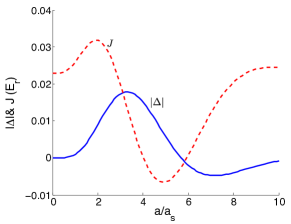
Figure 6: (Color online) The pairing amplitude $|\Delta|$ (solid line) and the hopping parameter $J$ (dashed line) in the Kitaev Hamiltonian in the units of the recoil energy as a function of the ratio $a/a_{s}$ between the lattice constant $a$ and the molecular size $a_{s}$, based on Eqs. (9) and (107) for $|\Delta|$ and Eqs. (103) and (108) for $J$. Other parameters are $\sigma_{x}\sigma_{\perp}^{2}/a^{3}=0.03$, and $n_{\text{M}}a_{s}^{3}=0.01$. The maximal value for the pairing amplitude $|\Delta|\sim 0.02E_{r}$ occurs for $a/a_{s}\sim 3$.

Figure 7: (Color online) The pairing amplitude $|\Delta|$ (solid line) and the hopping amplitude $J$ (dashed line) in the Kitaev Hamiltonian in units of the recoil energy as a function of the lattice depth $V_{x}$ for $a_{s}/a=1/3$ and $n_{\text{M}}a_{s}^{3}=0.01$. The optimal condition $|\Delta|\approx J$ for the localization of the Majorana modes is achieved for $V_{x}\sim 10E_{r}$.

Appendix B Majorana edge states in a finite Kitaev wire

We present in this Appendix a detailed derivation of the analytical expressions for the wave function and eigenenergy of the Majorana edge states in a finite Kitaev chain of $L$ sites with open boundary conditions, described by the Hamiltonian

$$H_{K}=\sum_{j=1}^{L-1}[-J\hat{a}_{j}^{{\dagger}}\hat{a}_{j+1}+\Delta\hat{a}_{j}\hat{a}_{j+1}+\text{h.c.}]-\sum_{j=1}^{L}\mu\hat{a}_{j}^{{\dagger}}\hat{a}_{j}.$$

Without loss of generality, we consider the hopping amplitude $J$ and the gap parameter $\Delta$ as real and positive. Our starting point is the Bogoliubov-de Gennes equations for the Bogoliubov amplitudes $u_{j,n}$ and $v_{j,n}$ at sites $j=1,...,L$,

$$-J(u_{j+1,n}+u_{j-1,n})-\mu u_{j,n}+\Delta(\upsilon_{j-1,n}-\upsilon_{j+1,n}) =E_{n}u_{j,n},$$

$$-J(\upsilon_{j+1,n}+\upsilon_{j-1,n})-\mu\upsilon_{j,n}+\Delta\left(u_{j-1,n}-u_{j+1,n}\right) =-E_{n}\upsilon_{j,n},$$ (109)

supplemented with the open boundary conditions

$$u_{0,n}=\upsilon_{0,n}=u_{L+1,n}=\upsilon_{L+1,n}=0.$$ (110)

Here, the definition of $u_{j,n}$ and $v_{j,n}$ has been formally extended to the sites $j=0$ and $j=L+1$. Next, we will look for the edge states $(u_{j,M},\upsilon_{j,M})$ with the energy $E_{M}$ that satisfy the BdG equations (109) under the boundary condition in Eq. (110), in the regime $|\mu|<2J$.

To this end, let us introduce new functions

$$f_{\pm,j}=u_{jM}\pm\upsilon_{jM}.$$ (111)

In terms of $f_{\pm,j}$, the BdG equations (109) is transformed into (for $j=1,...,L$)

$$-J\left(f_{+,j+1}\!+\!f_{+,j-1}\right)-\mu f_{+,j}+\Delta(f_{+,j-1}-f_{+,j+1}) =E_{M}f_{-,j},$$

$$-J\left(f_{-,j+1}\!+\!f_{-,j-1}\right)-\mu f_{-,j}-\Delta(f_{-,j-1}-f_{-,j+1}) =E_{M}f_{+,j},$$ (112)

which is supplemented with the corresponding open boundary conditions at $j=0$ and $j=L+1$

$$f_{\pm,0}=0,\hskip 17.07164ptf_{\pm,L+1}=0.$$ (113)

Equations (112) can be solved by the following ansatz

$$f_{+,j}=\alpha z^{j},\hskip 17.07164ptf_{-,j}=\beta z^{j}.$$ (114)

Substitution of Eqs. (114) into Eqs. (112) yields two coupled equations

$$F_{1}(z)\alpha+E_{M}\beta=0,\hskip 5.69054ptE_{M}\alpha+F_{2}(z)\beta=0,$$ (115)

with

$$\!\!\!\!F_{1}(z) =(J+\Delta)z\!+\mu\!+(J-\Delta)/z,$$ (116)

$$\!\!\!\!F_{2}(z) =(J-\Delta)z\!+\mu\!+(J+\Delta)/z\!=\!F_{1}(1/z).$$ (117)

From the condition for the existence of nonzero solutions $(\alpha,\beta)$ to Eq. (115), we immediately obtain

$$F_{1}(z)F_{2}(z)=E_{M}^{2}.$$ (118)

B.1 The case of $L\rightarrow\infty$

First, we consider the limiting case $L\rightarrow\infty$, for which $E_{M}=0$ is exact. Equation (115) can immediately be decoupled into two equations

$$F_{1}(z) =0,$$ (119)

$$F_{2}(z) =0,$$ (120)

which can be easily solved. Denoting the solutions to Eq. (119) as $z_{1},z_{2}$ and that to Eq. (120) as $z_{3},z_{4}$, we find

$$z_{1}=x_{+},\hskip 8.53581ptz_{2}=x_{-},\hskip 8.53581ptz_{3}=x_{+}^{-1},\hskip 8.53581ptz_{4}=x_{-}^{-1},$$

with

$$x_{\pm}=\frac{-\mu\pm\sqrt{\mu^{2}-4(J^{2}-\Delta^{2})}}{2(J+\Delta)}.$$ (121)

In the topological phase of the chain when $|\mu|<2J$, it follows from Eq. (121) that $|x_{\pm}|<1$. As a result, the solutions in Eq. (119), $z_{1,2}^{j}=x_{\pm}^{j}$, decay exponentially with increasing $j$; whereas, the solutions in Eq. (120), $z_{3,4}^{j}=x_{\pm}^{-j}$, decay exponentially with decreasing $j$. Therefore, we see that, for a Kitaev wire with $L\rightarrow\infty$, there exists an exact solution of BdG Eq. (112) corresponding $E_{M}=0$ with $f_{+,j}\sim(x_{+}^{j}-x_{-}^{j})$ and $f_{-.j}\sim(x_{+}^{L+1-j}-x_{-}^{L+1-j})$ that fulfill the boundary condition of Eq. (113).

B.2 The case of finite $L$

Now, we turn to the case when $L$ is finite but large, in which $E_{M}$ is nonzero but exponentially small. Since Eq. (118) cannot be decoupled for $E_{M}\neq 0$, the corresponding four solutions become $E_{M}$-dependent. Let us label these solutions as $z_{i}(E_{M})$ (for $i=1,2,3,4$), so that in the limit $E_{M}\rightarrow 0$ they approaches $z_{i}$ in an infinite wire, i. e. $z_{i}(E_{M}\rightarrow 0)=z_{i}$. Notice that, as $F_{1}(z)=F_{2}(1/z)$ from Eq. (117), we have the relation $z_{3}(E_{M})=1/z_{1}(E_{M})$ and $z_{4}(E_{M})=1/z_{2}(E_{M})$ between the pair of solutions $z_{1,2}(E_{M})$ and $z_{3,4}(E_{M})$. The exact expressions for $z_{i}(E_{M})$ can be found, by casting Eq. (118) into a quadratic equation $(J^{2}-\Delta^{2})y^{2}+4\mu Jy+(4\Delta^{2}+\mu^{2}-E_{M}^{2})=0$ for $y=z+z^{-1}$. However, they are very lengthy and will not be presented here.

Corresponding to each $z_{i}(E_{M})$, Equation (115) allows us to derive the ratio between $\alpha^{(i)}$ and $\beta^{(i)}$. Specifically, for the pair of solutions $z_{1,2}(E_{M})$, by noting $F_{1}\left(x_{\pm}\right)=0$ but $F_{2}\left(x_{\pm}\right)\neq 0$, we use Eq. (118) to obtain $F_{1}\left[z_{1,2}(E_{M})\right]=E_{M}^{2}/F_{2}\left[z_{1,2}(E_{M})\right]$, which is substituted into Eq. (115) to give (for $i=1,2$)

$${\beta}^{(i)}=-\frac{E_{M}}{F_{2}\left[z_{i}(E_{M})\right]}\alpha^{(i)}.$$ (122)

On the other hand, for the pair of solutions $z_{3,4}(E_{M})=1/z_{1,2}(E_{M})$, we recall $F_{2}\left(1/x_{\pm}\right)=0$ but $F_{1}\left(1/x_{\pm}\right)=F_{2}(x_{\pm})\neq 0$, and thus substitute $F_{2}\left[z_{3,4}(E_{M})\right]=E_{M}^{2}/F_{1}\left[z_{3,4}(E_{M})\right]$ into Eq. (115) to obtain (for $i=3,4$)

$${\alpha}^{(i)}=-\frac{E_{M}}{F_{1}\left[z_{i}(E_{M})\right]}{\beta}^{(i)}.$$ (123)

Now, we are readily to find the general solutions to Eq. (112) with Eqs. (114), (122) and (123). Keeping in mind that $z_{3}(E_{M})=1/z_{1}(E_{M})$ and $z_{4}(E_{M})=1/z_{2}(E_{M})$, we can express the general solutions of Eq. (112) as

$$f_{+,j} =\alpha^{(1)}z_{1}^{j}(E_{M})+\alpha^{(2)}z_{2}^{j}(E_{M})+\tilde{\alpha}^{(3)}z_{1}^{L+1-j}(E_{M})+\tilde{\alpha}^{(4)}z_{2}^{L+1-j}(E_{M}),$$

$$f_{-,j} =\beta^{(1)}z_{1}^{j}(E_{M})+\beta^{(2)}z_{2}^{j}(E_{M})+\tilde{\beta}^{(3)}z_{1}^{L+1-j}(E_{M})+\tilde{\beta}^{(4)}z_{2}^{L+1-j}(E_{M}),$$ (124)

with $\tilde{\alpha}^{(3)}={\alpha}^{(3)}/z_{1}^{L+1}$, $\tilde{\alpha}^{(4)}={\alpha}^{(4)}/z_{2}^{L+1}$, $\tilde{\beta}^{(3)}={\beta}^{(3)}/z_{1}^{L+1}$, and $\tilde{\beta}^{(4)}={\beta}^{(4)}/z_{2}^{L+1}$. In the limit $E_{M}\rightarrow 0$, Equations (124) naturally approaches the corresponding expressions in a $L\rightarrow\infty$ chain. After imposing the open boundary conditions in Eq. (110), we obtain the following equations

$$-\frac{E_{M}}{F_{2}\left[z_{1}(E_{M})\right]}\alpha^{(1)}-\frac{E_{M}}{F_{2}\left[z_{2}(E_{M})\right]}\alpha^{(2)}+z_{1}^{L+1}(E_{M})\tilde{\beta}^{(3)}+z_{2}^{L+1}(E_{M})\tilde{\beta}^{(4)} =0,$$ (125)

$$z_{1}^{L+1}(E_{M})\alpha^{(1)}+z_{2}^{L+1}(E_{M})\alpha^{(2)}-\frac{E_{M}}{F_{1}\left[z_{3}(E_{M}\right]}\tilde{\beta}^{(3)}-\frac{E_{M}}{F_{1}\left[z_{4}(E_{M}\right]}\tilde{\beta}^{(4)} =0,$$ (126)

$$\alpha^{(1)}+\alpha^{(2)}-\frac{E_{M}z_{1}^{L+1}(E_{M})}{F_{1}\left[z_{3}(E_{M})\right]}\tilde{\beta}^{(3)}-\frac{E_{M}z_{2}^{L+1}(E_{M})}{F_{1}\left[z_{4}(E_{M})\right]}\tilde{\beta}^{(4)} =0,$$ (127)

$$-\frac{E_{M}z_{1}^{L+1}(E_{M})}{F_{2}\left[z_{1}(E_{M})\right]}\alpha^{(1)}-\frac{E_{M}z_{2}^{L+1}(E_{M})}{F_{2}\left[z_{2}(E_{M}\right]}\alpha^{(2)}+\tilde{\beta}^{(3)}+\tilde{\beta}^{(4)} =0.$$ (128)

The resolutions of Eqs. (125)-(128) and the exact determination of $E_{M}$ are possible but very complicated. For our purpose, it suffices to noting the exponentially smallness of $E_{M}$ and thus seeking approximate solutions in the linear order of $E_{M}$. Keeping in mind $x_{\pm}^{L+1}\approx e^{-La/l_{M}}\sim E_{M}$, we ignore terms $\sim E_{M}^{2}$ and beyond, such that Eqs. (125)-(128) reduce to

$$-\frac{E_{M}}{s_{+}}\alpha^{(1)}-\frac{E_{M}}{s_{-}}\alpha^{(2)}+\tilde{\beta}^{(3)}x_{+}^{L+1}+\tilde{\beta}^{(4)}x_{-}^{L+1} =0,$$

$$\alpha^{(1)}x_{+}^{L+1}\!+\!\alpha^{(2)}x_{-}^{L+1}\!-\!\frac{E_{M}}{s_{+}}\tilde{\beta}^{(3)}\!-\!\frac{E_{M}}{s_{-}}\tilde{\beta}^{(4)} =0,$$

$$\alpha^{(1)}\!+\!\alpha^{(2)}=0,\tilde{\beta}^{(3)}+\tilde{\beta}^{(4)} =0,$$ (129)

where we have introduced $s_{\pm}=F_{2}\left[x_{\pm}\right]=F_{1}\left[x_{\pm}^{-1}\right]$ given by

$$s_{\pm}=\frac{2\Delta\left(\mu\Delta\pm J\sqrt{\mu^{2}-4(J^{2}-\Delta^{2})}\right)}{\Delta^{2}-J^{2}}.$$

Consequently by solving Eq. (129), we can obtain the eigenenergy

$$E_{M}=\Big{|}\frac{\Delta(4J^{2}-\mu^{2})(x_{+}^{L+1}-x_{-}^{L+1})}{J(\Delta+J)(x_{+}-x_{-})}\Big{|},$$ (130)

and the corresponding eigenfunctions

$$f_{+,j} =A\Big{[}x_{+}^{j}-x_{-}^{j}-\frac{E_{M}}{s_{+}}x_{+}^{L+1-j}+\frac{E_{M}}{s_{-}}x_{-}^{L+1-j}\Big{]},$$

$$f_{-,j} =A\Big{[}x_{+}^{L+1-j}\!-\!x_{-}^{L+1-j}\!-\!\frac{E_{M}}{s_{+}}x_{+}^{j}+\frac{E_{M}}{s_{-}}x_{-}^{j}\Big{]}.$$ (131)

We emphasize that $f_{\pm,j}$ in Eq. (131) fulfills the open boundary condition in Eq. (110) approximately (to the order of $\sim E_{M}^{2}$). As is manifest from Eq. (131), for large but finite $L$, $f_{+,j}$ is localized near the left edge but involves small admixture (at the order $\sim E_{M}$) from $x_{\pm}^{L+1-j}$ which decays from the right edge, while $f_{-,j}$ is localized near the right end with small admixtures ($\sim E_{M}$) from $x_{\pm}^{j}$ that decays from the left. The coefficient $A$ in Eq. (131) can be determined from the renormalization condition $\sum_{j}|u_{jM}|^{2}+|\upsilon_{jM}|^{2}=1$ (ignoring terms $\sim E_{M}^{2}$). In this way, we obtain

$$A=\sqrt{\frac{\Delta(4J^{2}-\mu^{2})}{J(\mu^{2}+4\Delta^{2}-4J^{2})}},$$ (132)

for $\mu^{2}-4(J^{2}-\Delta^{2})>0$, when $x_{\pm}$ and $s_{\pm}$ are real; and

$$A=-i\sqrt{\frac{\Delta(4J^{2}-\mu^{2})}{J(4J^{2}-4\Delta^{2}-\mu^{2})}},$$

for $4(J^{2}-\Delta^{2})-\mu^{2}>0$, when $x_{+}=x_{-}^{\star}=(-\mu+i\sqrt{4J^{2}-4\Delta^{2}-\mu^{2}})/2(\Delta+J)$ and $s_{+}^{\ast}=s_{-}$. Consequently, in both regimes, the resulting $f_{\pm,j}$ are real. Having found $f_{\pm,j}$, we can obtain the expressions for $u_{j,M},\upsilon_{j,M}$ ( in the linear order of $E_{M}$) from Eq. (111). The results are

$$u_{jM} = \frac{A}{2}\Big{[}(1-\frac{E_{M}}{s_{+}})(x_{+}^{j}+x_{+}^{L+1-j})-(1-\frac{E_{M}}{s_{-}})(x_{-}^{j}+x_{-}^{L+1-j})\Big{]},$$

$$\upsilon_{jM} = \frac{A}{2}\Big{[}(1-\frac{E_{M}}{s_{+}})(x_{+}^{j}-x_{+}^{L+1-j})-(1-\frac{E_{M}}{s_{-}})(x_{-}^{j}-x_{-}^{L+1-j})\Big{]}.$$ (133)

Now, the Majorana wave functions $f_{L/R,j}$ can be readily derived using Eq. (133) according to the main text. Since $f_{\pm,j}$ can always be made real, we have $f_{L,j}=f_{+,j}$ and $f_{R,j}=f_{-,j}$. Let us illustrate our results in the considered regime $\mu^{2}-4(J^{2}-\Delta^{2})<0$, in which it is more convenient to write $x_{\pm}=\rho e^{\pm i\theta}$ with $\rho=\sqrt{(J-\Delta)/(J+\Delta)}$ and $\theta=\arccos[-\mu/2\sqrt{J^{2}-\Delta^{2}}]$. The Majorana wave function $f_{j,L/R}$ can then be written (in the leading order $E_{M}$) as

$$f_{Lj} =2\left|A\right|\rho^{j}\sin(j\theta),$$

$$f_{Rj} =2\left|A\right|\rho^{L-j+1}\sin[(L-j+1)\theta];$$ (134)

and the energy, Eq. (130), as

$$E_{M} =\Delta\rho^{L}\frac{4J^{2}-\mu^{2}}{J(\Delta+J)}\Big{|}\frac{\sin[(L+1)\theta]}{\sin\theta}\Big{|}$$

$$=\Delta e^{-La/l_{M}}\frac{4J^{2}-\mu^{2}}{J(\Delta+J)}\Big{|}\frac{\sin[(L+1)\theta]}{\sin\theta}\Big{|}.$$ (135)

We thus clearly see that the energy of the edge mode decays exponentially with $L$, and the localization length of the Majorana wave functions near the edges is

$$l_{M}=\frac{a}{\ln\rho^{-1}}=\frac{a}{\ln(\sqrt{(J+\Delta)/(J-\Delta})}.$$

As an example, consider the case of $\mu=0$ and $J\neq\Delta$, when Eq. (135) indicates $E_{M}=0$ when $L$ is odd. In fact, $E_{M}=0$ is an exact result for $\mu=0$ and odd $L$, which can be most easily seen by expressing the Kitaev Hamiltonian in the Majorana basis Kitaev . In this basis, the Hamiltonian matrix $(2L\times 2L)$ For $\mu=0$ can be brought into a a block diagonal form $H_{\mathrm{K}}=H_{1}\oplus H_{2}$, in which $H_{1}$ matrix couples Majorana operators $(c_{4n+1},c_{4n+4})$ and $H_{2}$ matrix couples Majorana operators $(c_{4n+2},c_{4n+3})$, respectively, for $n=0,1,2..$. Both $H_{1}$ and $H_{2}$ matrices are antisymmetric and are of dimension $L$, such that we can immediately infer the existence of the zero energy-eigenvalue when $L$ is odd.

B.3 Bulk correlations

Let us also calculate some correlations functions in the bulk of the wire, which are determined by the gapped modes. In the thermodynamic limit $L\rightarrow\infty$, the bulk gapped modes can be characterized by their quasi-momentum $\hbar k$ from the Brillouin zone (BZ), $k\in[-\pi/a,\pi/a]$, with the corresponding energy $E_{k}=\sqrt{(2J\cos ka+\mu)^{2}+4\Delta^{2}\sin^{2}ka}$. In this case, Eq. (18) takes the form

$$a_{j}^{\prime}=\frac{1}{\sqrt{L}}\sum_{k\in\mathrm{BZ}}(u_{k}\alpha_{k}e^{ikaj}+v_{k}^{\ast}\alpha_{k}^{{\dagger}}e^{-ikaj}),$$ (136)

where

$$u_{k}=\sqrt{\frac{E_{k}+\xi_{k}}{2E_{k}}},\;v_{k}=i\frac{2\Delta\sin ka}{E_{k}+\xi_{k}}u_{k}=\frac{2i\Delta\sin ka}{\sqrt{2E_{k}(E_{k}+\xi_{k})}}$$ (137)

satisfy the condition $u_{k}^{2}+\left|v_{k}\right|^{2}=1$ and $\xi_{k}=-2J\cos ka-\mu$.

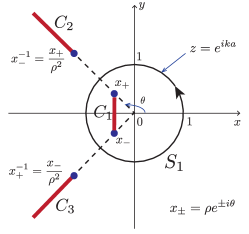
Figure 8: Contour of the integration $\mathrm{S}_{1}$ in the complex $z$-plane, four brancing points $x_{\pm}$ and $x_{\pm}^{-1}$, and three cuts $C_{1}$, $C_{2}$, and $C_{3}$ defining the branch of the function $\sqrt{F_{1}(z)F_{2}(z)}$.

We start with the correlation function $f(r)\equiv\left\langle a_{j+r}^{\prime}a_{j}^{\prime}\right\rangle=-f(-r)$ which can be written as

$$f(r)=\left\langle a_{j+r}^{\prime}a_{j}^{\prime}\right\rangle=\frac{1}{L}\sum_{k\in\mathrm{BZ}}u_{k}v_{k}^{\ast}e^{ikar}=-\int_{-\pi}^{\pi}\frac{d\widetilde{k}}{2\pi}\frac{2i\Delta\sin\widetilde{k}}{2E_{\widetilde{k}}}e^{i\widetilde{k}r},$$

where $\widetilde{k}=ka$. After introducing the complex variable $z=\exp(i\widetilde{k})$, the expression for $f(r)$ can be rewritten as a contour integral over the unit circle S₁ in the complex $z$-plane (see Fig. 8):

$$f(r)=-\frac{\Delta}{2\pi}\oint_{\mathrm{S}_{1}}\frac{dz}{iz}\frac{(z-z^{-1})}{2\sqrt{F_{1}(z)F_{2}(z)}}z^{r}$$

with $F_{1}(z)$ and $F_{2}(z)$ being defined in Eqs. (116) and (117), respectively. Note that the integrand in the above expression has four branching points $x_{+}$, $x_{-}$, $x_{+}^{-1}=x_{-}/\rho^{2}$, and $x_{-}^{-1}=x_{+}/\rho^{2}$ [zeros of $F_{1}(z)$ and $F_{2}(z)$], and the branch of this multivalued function is specified by making three cuts C₁, C₂, and C₃ in the complex plane, see Fig. 8. After simple manipulations, the integral can be rewritten in the form

$$f(r)=-\frac{1}{2\pi}\frac{\alpha}{2\sqrt{1-\alpha^{2}}}\oint_{\mathrm{S}_{1}}\frac{dz}{iz}\frac{(z^{2}-1)}{\sqrt{(z-x_{+})(z-x_{-})(z-x_{+}^{-1})(z-x_{-}^{-1})}}z^{r},$$

where $\alpha=\Delta/J<1$. Without loss of generality, we consider $r>0$ and deform S₁ to the contour around the cut C₁ which connects the points $x_{+}$ and $x_{-}$. To simplify the calculations we consider the case $1-\alpha^{2}\ll 1$, when $\rho=\left|x_{\pm}\right|\ll 1$ and $\left|z\right|\ll 1$ for $z\in$C₁, and, using the approximate expression for $(z-x_{+}^{-1})(z-x_{-}^{-1})\approx(x_{+}x_{-})^{-1}=\rho^{-2}$ for $z\in$C₁, simplify the integral to the form

$$f(r)=\frac{1}{2\pi}\frac{\alpha}{2(1+\alpha)}\oint_{\mathrm{C}_{1}}\frac{dz}{iz}\frac{1}{\sqrt{(z-x_{+})(z-x_{-})}}z^{r}.$$

After writing

$$z(y)=\frac{1}{2}(x_{+}+x_{-})+\frac{y}{2}(x_{+}-x_{-})=\rho(\cos\theta+iy\sin\theta)\in\mathrm{C}_{1},$$

where $y\in[-1,1]$, we find (the value of the function $\sqrt{(z-x_{+})(z-x_{-})}$ is chosen to be positive on the right side of the cut)

$$f(r) = \frac{1}{2\pi}\frac{\alpha}{1+\alpha}\rho^{r-1}\int_{-1}^{1}\frac{dy}{\sqrt{1-y^{2}}}(\cos\theta+iy\sin\theta)^{r-1}$$

$$= \frac{1}{2}\frac{\alpha}{1+\alpha}\rho^{r-1}\mathrm{P}_{r-1}(\cos\theta),$$

where $\mathrm{P}_{n}(x)$ is the Legendre polynomial of degree $n$. The asymptotics of $f(r)$ for large $r,$

$$f(r\gg 1)\approx\frac{1}{2}\frac{\alpha}{1+\alpha}\sqrt{\frac{2}{\pi r\sin\theta}}\rho^{r-1}\cos[(r-1/2)\theta-\pi/4],$$ (139)

shows exponential decay with the characteristic length $\xi_{BCS}=l_{M}=-a\ln\rho$.

The correlation function

$$g(r)=\left\langle a_{j+r}^{\prime{\dagger}}a_{j}^{\prime}\right\rangle=g(-r)=\frac{1}{L}\sum_{k\in\mathrm{BZ}}\left|v_{k}\right|^{2}e^{ikar}=\int_{-\pi}^{\pi}\frac{d\widetilde{k}}{2\pi}\frac{1}{2}\left(1+\frac{\xi_{\widetilde{k}}}{E_{\widetilde{k}}}\right)e^{i\widetilde{k}r}$$ (140)

can be calculated in the same way (we again consider the case $1-\alpha^{2}\ll 1$, that is $\rho\ll 1$): For $r\geq 1$ we obtain

$$g(r)=\frac{1}{2}\frac{1}{1+\alpha}\rho^{r-1}\mathrm{P}_{r-1}(\cos\theta)$$ (141)

or asymptotically

$$g(r\gg 1)\approx\frac{1}{2}\frac{1}{1+\alpha}\sqrt{\frac{2}{\pi r}}\left(\frac{1-\alpha^{2}}{1-\alpha^{2}-\beta^{2}}\right)^{1/4}\rho^{r-1}\cos[(r-1/2)\theta-\pi/4].$$ (142)

Finally, we calculate the correlation function

$$h(r)=\frac{1}{L}\sum_{k\in\mathrm{BZ}}\frac{(u_{k}+v_{k})^{2}\sin^{2}ka}{E_{k}}e^{ikar}$$ (143)

which appears in the temperature-dependent correction to the energy of the Majorana mode, Eq. (62). After using the expressions for $u_{k}$ and $v_{k}$ from Eq. (137) and dimensional variable $\widetilde{k}=ka$, the expression for $h(r)$ reads

$$h(r)=\int_{-\pi}^{\pi}\frac{d\widetilde{k}}{2\pi}\frac{\xi_{\widetilde{k}}+2i\Delta\sin\widetilde{k}}{E_{\widetilde{k}}^{2}}\sin^{2}\widetilde{k}\;e^{i\widetilde{k}r}=\int_{-\pi}^{\pi}\frac{d\widetilde{k}}{2\pi}\frac{\sin^{2}\widetilde{k}}{\xi_{\widetilde{k}}-2i\Delta\sin\widetilde{k}}e^{i\widetilde{k}r},$$

where we use the identity $E_{\widetilde{k}}^{2}=(\xi_{\widetilde{k}}+2i\Delta\sin\widetilde{k})(\xi_{\widetilde{k}}-2i\Delta\sin\widetilde{k})$. The last integral can be transformed into the contour integral in the complex $z$-plane as

$$h(r)=\frac{1}{2\pi}\oint_{\mathrm{S}_{1}}\frac{dz}{iz}\frac{(z-z^{-1})^{2}}{4F_{1}(z)}z^{r}=\frac{1}{4J(1+\alpha)}\oint_{\mathrm{S}_{1}}\frac{dz}{2\pi i}\frac{1}{z^{2}}\frac{(1-z^{2})^{2}}{(z-x_{+})(z-x_{-})}z^{r},$$

and then calculated by deforming the contour of integration and using the Cauchy theorem: For $r<-1$, we deform the contour to infinity with zero result for the integral; for $r\geq-1$, the contour is deformed to zero and the result of the integration is given by the contribution of the poles at $z=x_{+}$, $z=x_{-}$, and $z=0$ (for $r=0$, $\pm 1$). After calculating the corresponding residues we obtain

$$h(r) = \frac{1}{4J}\frac{(1-x_{+}^{2})^{2}x_{+}^{r-2}-(1-x_{-}^{2})^{2}x_{-}^{r-2})}{2i\sqrt{1-\alpha^{2}-\beta^{2}}}$$

$$= \frac{1}{4J(1+\alpha)}\frac{\rho^{r-3}}{\sin\theta}\left\{\sin[(r-2)\theta]-2\rho^{2}\sin(r\theta)+\rho^{4}\sin[(r+2)\theta]\right\},\hskip 5.69054ptr>1$$

$$h(1) = -\frac{1}{4J(1+\alpha)}\left[1+2\frac{1+\alpha-2\beta^{2}}{(1+\alpha)^{2}}\right]=\frac{1}{4J(1+\alpha)}[-2+\rho^{2}(4\cos^{2}\theta-1)],$$

$$h(0) = -\frac{\beta}{2J(1+\alpha)^{2}}=\frac{1}{4J(1+\alpha)}2\rho\cos\theta,$$

$$h(-1) = \frac{1}{4J(1+\alpha)},$$

$$h(r) = 0,\hskip 5.69054ptr<-1,$$ (144)

where we $\alpha=\Delta/J$ and $\beta=\mu/2J$. Note that this correlation function behaves differently for positive and negative $r$ due to the specific analytical structure of the integrand. The replacement of $(u_{k}+v_{k})^{2}$ with $(u_{k}-v_{k})^{2}$ in the $h(r)$ results in the reflected ($r\rightarrow-r$) behavior.

The above expressions for the correlation functions show that the bulk correlation length $\xi_{BCS}$ is identical with the localization length of the Majorana edge states $l_{M}$. Mathematically it follows from the fact that both lengths originates from the zeros $x_{+}$ and $x_{-}$ of $E_{k}$ [or $F_{1}(z)F_{2}(z)$] in the complex plane of $z=\exp(ika)$.

References

(1) F. Wilczek, Nat. Phys. 5, 614 (2009).
(2) C. Nayak, Steven H. Simon, A. Stern, M. Freedman,
and S. Das Sarma, Rev. Mod. Phys. 80, 1083 (2008).
(3) A. Stern, Ann. Phys. 323, 204 (2008).
(4) A. Stern, Nature (London) 464, 187 (2010).
(5) A. Kitaev, Ann. Phys. (Amsterdam) 303, 2 (2003).
(6) M. H. Freedman, A. Kitaev, J. Larsen, and Z. Wang, Bull. Am.
Math. Soc. 40, 31 (2003).
(7) S. Das Sarma, M. Freedman, and C. Nayak, Phys. Rev. Lett.
94, 166802 (2005).
(8) J. K. Pachos, Introduction to Topological Quantum
Computation (Cambridge University Press, Cambridge, England, 2012).
(9) G. Moore and N. Read, Nucl. Phys. B360 , 362
(1991).
(10) N. Read and D. Green, Phys. Rev. B 61, 10267
(2000).
(11) D. A. Ivanov, Phys. Rev. Lett. 86, 268 (2001).
(12) A. Kitaev, Phys. Usp. 44, 131 (2001).
(13) M. Cheng and H. H. Tu, Phys. Rev. B 84, 094503
(2011).
(14) J. Alicea, Rep. Prog. Phys. 75, 076501 (2012)
(15) C. W. J. Beenakker, Annu. Rev. Condens. Matter Phys.
4, 113 (2013)
(16) T. D. Stanescu and S. Tewari, J. Phys.: Condens.
Matter 25, 233201 (2013).
(17) L. Fu and C. L. Kane, Phys. Rev. Lett. 100,
096407 (2008); Phys. Rev. B 79, 161408(R) (2009).
(18) J. D. Sau, R. M. Lutchyn, S. Tewari, and S. Das Sarma,
Phys. Rev. Lett. 104, 040502 (2010).
(19) R. M. Lutchyn, J. D. Sau, and S. Das Sarma, Phys. Rev.
Lett. 105, 077001 (2010).
(20) J. Alicea, Phys. Rev. B 81, 125318 (2010).
(21) Y. Oreg, G. Refael, and F. von Oppen, Phys. Rev. Lett.
105, 177002 (2010).
(22) L. Jiang, T. Kitagawa, J. Alicea, A. R. Akhmerov, D.
Pekker, G. Refael, J. I. Cirac, E. Demler, M. D. Lukin, and P. Zoller, Phys.
Rev. Lett. 106, 220402 (2011).
(23) S. Nascimbene, J. Phys. B: At. Mol. Opt. Phys 46, 134005 (2013).
(24) S. Diehl, E. Rico, M. A. Baranov, and P. Zoller, Nat.
Phys. 7, 971 (2011).
(25) C. V. Kraus, S Diehl, P. Zoller, and M. A. Baranov, New
J. Phys. 14, 113036 (2012).
(26) B. Sundar and E. J. Mueller, Phys. Rev. A 88,
063632 (2013).
(27) A. Bühler, N. Lang, C.V. Kraus, G. Möller, S. D.
Huber, and H.P. Büchler, Nat. Commun. 5, 4504 (2014)
(28) V. Mourik, K. Zuo, S. M. Frolov, S. R. Plissard, E. P. A.
M Bakkers, and L.P. Kouwenhoven, Science 336, 1003 (2012).
(29) M. T. Deng, C. L. Yu, G. Y. Huang, M. Larson, P. Caroff,
and H. Q. Xu, Nano Lett. 12, 6414 (2012).
(30) L. P. Rokhinson, X. Liu, and J. K. Furdyna, Nat. Phys.
8, 795 (2012).
(31) A. Das, Y. Ronen, Y. Most, Y. Oreg, M. Heiblum, and H.
Shtrikman, Nat. Phys. 8, 887 (2012).
(32) H. O. H. Churchill, V. Fatemi, K. Grove-Rasmussen,
M. T. Deng, P. Caroff, H. Q. Xu, and C. M. Marcus, Phys. Rev.
B 87, 241401(R) (2013).
(33) A. D. K. Finck, D. J. Van Harlingen, P. K. Mohseni, K.
Jung, and X. Li, Phys. Rev. Lett. 110, 126406 (2013).
(34) S. Nadj-Perge, I. K. Drozdov, J. Li, H. Chen, Sangjun
Jeon, Jungpil Seo, A. H. MacDonald, B. A.Bernevig, A. Yazdani, Science
346, 602 (2014).
(35) A.A. Zyuzin, D. Rainis, J. Klinovaja, and D. Loss, Phys.
Rev. Lett. 111, 056802 (2013).
(36) I. Bloch, J. Dalibard, and W. Zwerger, Rev.
Mod. Phys. 80, 885 (2008).
(37) D. S. Petrov, C. Salomon, and G. V.
Shlyapnikov, Phys. Rev. Lett. 93, 090404 (2004).
(38) D. S. Petrov, Phys. Rev. A 67, 010703 (2003).
(39) A. L. Fetter and J. D. Walecka, Quantum Theory of
Many-Particle Systems, (McGraw-Hill Book Company, New York, 1971).
(40) C. V. Kraus, P. Zoller, and M. A. Baranov, Phys. Rev.
Lett. 111, 203001 (2013).
(41) C. Laflamme, M. A. Baranov, P. Zoller, and C. V. Kraus
Phys. Rev. A 89, 022319 (2014).
(42) W. Ketterle and M. W. Zwierlein, Rivista del Nuovo
Cimento 31, 247-422 (2008).