A 1.3 cm line survey toward IRC +10216

Abstract

Context. IRC +10216 is the prototypical carbon star exhibiting an extended molecular circumstellar envelope. Its spectral properties are therefore the template for an entire class of objects.

Aims. The main goal is to systematically study the $\lambda$ $\sim$1.3 cm spectral line characteristics of IRC +10216.

Methods. We carried out a spectral line survey with the Effelsberg-100 m telescope toward IRC +10216. It covers the frequency range between 17.8 GHz and 26.3 GHz (K-band).

Results. In the circumstellar shell of IRC +10216, we find 78 spectral lines, among which 12 remain unidentified. The identified lines are assigned to 18 different molecules and radicals. A total of 23 lines from species known to exist in this envelope are detected for the first time outside the Solar System and there are additional 20 lines first detected in IRC +10216. The potential orgin of “U” lines is also discussed. Assuming local thermodynamic equilibrium (LTE), we then determine rotational temperatures and column densities of 17 detected molecules. Molecular abundances relative to H₂ are also estimated. A non-LTE analysis of NH₃ shows that the bulk of its emission arises from the inner envelope with a kinetic temperature of 70$\pm$20 K. Evidence for NH₃ emitting gas with higher kinetic temperature is also obtained, and potential abundance differences between various ¹³C-bearing isotopologues of HC₅N are evaluated. Overall, the isotopic ¹²C/¹³C ratio is estimated to be 49$\pm$9. Finally, a comparison of detected molecules in the $\lambda$ $\sim$1.3 cm range with the dark cloud TMC-1 indicates that silicate-bearing molecules are more predominant in IRC +10216.

1 Introduction

Molecular line surveys are a powerful tool for analyzing both physical and chemical parameters of astronomical objects. In fact, they are the only means of obtaining a complete, unbiased view of the molecular inventory of a given source. However, despite the long history of powerful large radio telescopes, few unbiased frequency surveys have been conducted in the cm-wave regime. A 4.4 GHz bandwidth survey from 17.6 to 22.0 GHz toward the massive star-forming region W51 has been reported by Bell et al. (1993b) showing many previously unidentified lines. The dark cloud TMC-1 has been observed in selected bands from 4-6 and 8-10 GHz (Kalenskii et al. 2004), as well as at 9-50 GHz (Kaifu et al. 2004). More recently, some systematic observations toward the galactic center have also been reported by Remijan et al. (2008) in the course of their GBT PRIMOS project.

Spectroscopic features that are expected at long wavelengths (i.e. in the cm-wave regime) include recombination lines from HI, HeI, and CI, which can be assigned in a straightforward manner. In addition, complex molecules have small rotational constants so that their lowest-energy transitions arise at cm-wavelenths. In this way, emission or absorption features from long carbon-chain molecules can be observed (e.g. HC₃N, HC₅N, HC₇N, HC₉N). Since systematic and highly sensitive surveys at these (low) frequencies that cover different sources have rarely been carried out, one can only speculate as to what else may be observed. The enormous potential of cm-wave astronomy for detecting new molecules in space has been highlighted in the recent past through GBT detections of complex organic molecules such as CH₂CHCHO (propenal), CH₃CH₂CHO (propanal), and CNCHO (cyanoformaldehyde) (Hollis et al. 2004; Remijan et al. 2008).

For this paper, we performed a 1.3 cm line survey toward IRC +10216, which is also known as CW Leonis. It is found to be the brightest object outside the Solar System at 5 $\mu$m (Becklin et al. 1969). It is a well-studied asymptotic giant branch (AGB) carbon star with a high mass loss rate (2.0 $\times\leavevmode\nobreak\ 10^{-5}$M_⊙yr^-1) at a distance of $\sim$130 pc (Crosas & Menten 1997; Menten et al. 2012), which results in a dense circumstellar envelope (CSE). The CSE is the ideal target for studying gas-phase chemistry in a peculiar, namely carbon-rich environment. Existing surveys, summarized in Table 1, cover parts of the frequency range from 4 GHz to 636.5 GHz for IRC +10216. These efforts have resulted in the discovery of over 70 species toward this object, including unusual carbon-chain molecules, metal cyanides such as MgNC, NaCN, and AlNC (Cernicharo et al. 2000a; Ziurys et al. 2002), and even metal halides: NaCl, AlCl, KCl, and AlF (Cernicharo & Guelin 1987). However, the frequency range between 18 and 26 GHz is still largely unexplored. Here, we therefore systematically study the characteristics of IRC+10216 in the important $\lambda$ $\sim$1.3 cm (K-band) spectral range, which is known to contain a number of lines from prominent molecules like H₂O, NH₃, and the cyanopolyynes.

Table 1: Existing line surveys of IRC +10216.

Covered frequencies	Telescope	Reference
IRC +10216
4-6 GHz	Arecibo	Araya et al. (2003)
17.8-26.3 GHz	Effelsberg-100m	This work
28-50 GHz	Nobeyama-45m	Kawaguchi et al. (1995)
72-91 GHz	Onsala-20m	Johansson et al. (1984, 1985)
129-172.5 GHz	IRAM-30m	Cernicharo et al. (2000a)
131.2-160.3 GHz	ARO-12m	He et al. (2008)
215-285 GHz	SMT-10m	Tenenbaum et al. (2010)
219.5-245.5 GHz and 251.5-267.5 GHz	SMT-10m	He et al. (2008)
293.9-354.8 GHz	SMA	Patel et al. (2011)
330-358 GHz	CSO-10m	Groesbeck et al. (1994)
222.4-267.9 GHz and 339.6-364.6 GHz	JCMT-15m	Avery et al. (1992)
554.5-636.5 GHz	Herschel/HIFI	Cernicharo et al. (2010)

2 Observations and data reduction

The observations were carried out in a position-switching mode with the primary focus $\lambda$ = 1.3 cm K-band receiver of the 100-m telescope at Effelsberg/Germany, during 2012 in January, April, and 2013 in January, March, and May. On- and off-source integration times were two minutes per scan. The newly installed Fast Fourier Transform Spectrometer (FFTS) was used as backend. Each spectrometer, covering one of the two orthogonal linear polarizations with a bandwidth of 2 GHz provides 32768 channels, resulting in a channel spacing of 61 kHz, equivalent to 0.7 km s^-1at 26 GHz. The actual frequency and velocity resolutions are coarser by a factor of 1.16 (Klein et al. 2012). Several frequency setups were tuned to cover the entire frequency range from 17.8 GHz to 26.3 GHz with an overlap of at least 100 MHz between two adjacent frequency setups. Across the whole frequency range, the beamsize is 35″-50″($\sim$40″at 23 GHz). The survey encompasses a total of $\sim$ 130 observing hours. The focus was checked every few hours, in particular after sunrise and sunset. Pointing was obtained every hour toward the quasar PG 0851+202 (OJ +287) and was found to be accurate to about 5″. Strong continuum sources (mostly 3C286) were also used to calibrate the spectral line flux according to their standard flux densities (Ott et al. 1994). The typical rms noise is about $1-3$ mJy in $\sim$ 0.7 km s^-1 wide channels. In view of the width of the IRC +10216 spectra, $\sim$ 30 km s^-1, smoothed spectra typically reach rms noise levels of about 1 mJy. The conversion factor from Jy on a flux density scale ($S_{\nu}$) to K on a main beam brightness temperature scale ($T_{\rm mb}$) is $T_{\rm mb}/S_{\nu}\sim 1.5\leavevmode\nobreak\ {\rm K/Jy}$ at 22 GHz.

For the data reduction, the GILDAS software package including CLASS and GREG was employed. During the data reduction, some inevitable defects occured at the edges of the spectra. Therefore 100 channels at each edge were excluded. Fourth- to tenth-order baselines were subtracted from each spectrum with 2000 to 3000 channels to avoid lines being truncated at the edge of subspectra, and then these subspectra were stitched together to resconstruct the complete spectrum. Since some of the subspectra suffer contamination from time variable radio frequency interference (RFI), the channels showing RFI signals have been “flagged”, i.e. discarded from further analysis, resulting in some limited gaps in the averaged spectra. Furthermore, there were a few individual bad channels, which have also been eliminated.

3 Results

3.1 Line identifications

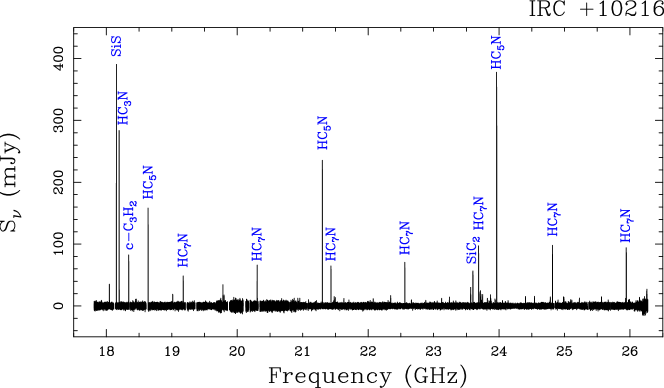
Figure 1: Overview of the 1.3 cm line survey toward IRC +10216 with strong lines marked.

The line identification was performed on the basis of the JPL, CDMS, and splatalogue databases as well as on the online Lovas line list for astronomical spectroscopy (Müller et al. 2005; Pickett et al. 1998; Lovas & Dragoset 2004). A line is identified as real if it is characterized by a signal-to-noise ratio of at least five. Figure 1 presents an overview of our $\lambda\sim$1.3 cm line survey toward IRC +10216. We find 78 spectral lines, among which 12 remain unidentified. The identified lines are assigned to 18 different molecules. Except for SiS and NH₃, they are all C-bearing molecules. Twenty-three lines from already known species are detected for the first time outside the Solar System and there are additional 20 lines first detected in IRC +10216. Details are described in Sect. 3.2.

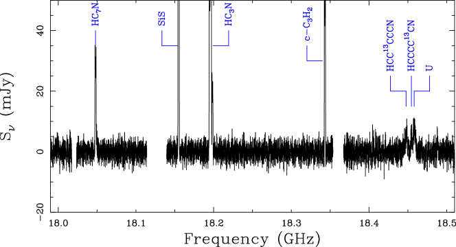
Figure 8: Observed spectrum of IRC $+$10216 from 17.8 to 26.3 GHz.

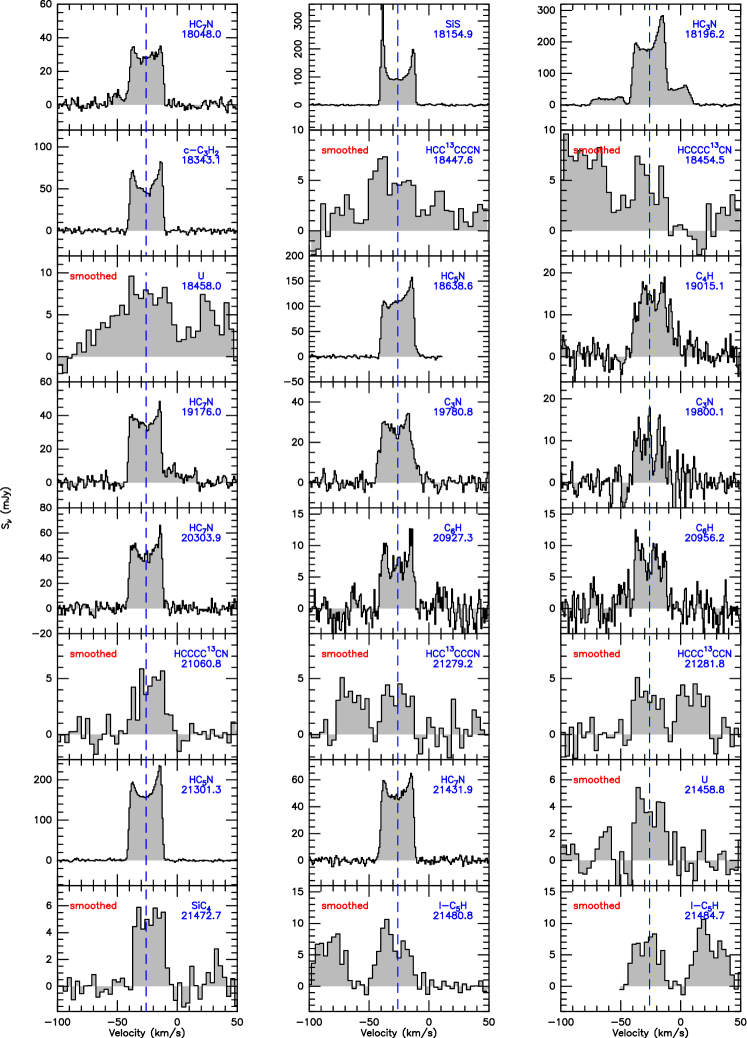
Figure 9: Zoom in all detected and tentative lines. The rest frequency in MHz and the assigned molecule of each line are shown in the upper right of each panel. Weak lines have been smoothed to have a channel width of $\sim$3.3 km s^-1, and they are marked with “smoothed” in the upper left of the corresponding panels. Otherwise, the channel width is $\sim$0.8 km s^-1(see Sect. 3.1). The blue dashed line traces the systemic LSR velocity ($-$26.0 km s^-1) of IRC +10216. In the C₆H 23565.2 MHz panel, the other blue dashed line near $-$50 km s^-1 refers to the C₆H’s hfs component at 23567.2 MHz.

The spectrum is dominated by the strong profiles from six species: SiS, HC₃N, and HC₅N with $S_{\nu}>100$ mJy; HC₇N, c-C₃H₂, and SiC₂ with $S_{\nu}>20$ mJy. Figure 8 shows the observed spectrum in more detail. Each panel covers $\sim$500 MHz of the spectrum. Furthermore, there is a 10 MHz overlap between adjacent panels so that lines truncated in one panel will not be truncated in the other panel. In addition, Fig. 9 shows zoom-in plots of all detected transitions.

We used the SHELL fitting routine in CLASS to derive the line parameters including peak intensity, integrated intensity, and expansion velocity, which is defined as the half-width at zero power. For the lines with hyperfine structure (hfs, like HC₃N, NH₃, etc.), only their main components are fitted with the routine to obtain their expansion velocities. For the lines that are blended or weak, the parameters are estimated directly by integrating the line profiles. The observed properties of the lines are displayed in Table LABEL:Tab:irclines. The fitted lines reveal an expansion velocity of around 14.0 km s^-1, which is consistent with previous studies (e.g., Cernicharo et al. 2000b; He et al. 2008). There are some previously reported narrow lines with expansion velocities of $<$ 10 km s^-1  that are mainly from high-$J$ transitions in the ground vibrational state or from transitions in vibrationally excited states (Patel et al. 2009; He et al. 2008), originating in the innermost, not yet fully accelerated shell. Lines with expansion velocities $<$ 10 km s^-1  are not seen in our study.

3.2 Newly detected lines

In the following, we briefly describe most of the 23 newly detected lines (denoted by an “N” in the last column of Table LABEL:Tab:irclines) and most of the other 20 lines newly detected in IRC +10216 (“NS”), together with related, already detected transitions from the same species. These transitions belong to HC₅N, HC₇N, HC₉N, SiC₄, NH₃, MgNC,  l-C₅H, C₆H, C₆H^-, and C₈H. The ¹³C-bearing isotopologues of HC₅N are also briefly addressed (see also Sect. 4.4).

HC₅N. – There are three transitions of cyanobutadiyne (HC₅N) in our observed frequency range. All of them have been detected, and the HC₅N line intensities rise with increasing frequency. HC₅N (9–8) has been reported by Winnewisser & Walmsley (1978), but their peak intensity is almost twice the peak intensity measured by us even though their data were also obtained at Effelsberg. Significant variations in line intensities measured at submm and far-infrared wavelengths have recently been reported by Cernicharo et al. (2014). However, unpublished HC₅N and HC₇N monitoring observations at Effelsberg about 25 yr ago (C. Henkel, priv. comm) did not reveal time variability in excess of 20%. Furthermore, the $\lambda\sim 3$ mm data of Cernicharo et al. (2014) also show no strong variability. This, as well as other discrepancies outlined below, are therefore very likely caused by narrower bandwidths, lower quality baselines, and noise diodes with a more frequency-dependent output, thus resulting in a less accurate calibration than we have obtained here.

¹³C-bearing HC₅N isotopologues. – We have detected 11 transitions from the ¹³C-bearing isotopologues of HC₅N. Seven of them are first detected outside the Solar System, while four other transitions have already been studied with the NRAO-43m telescope (Bell & Feldman 1991).

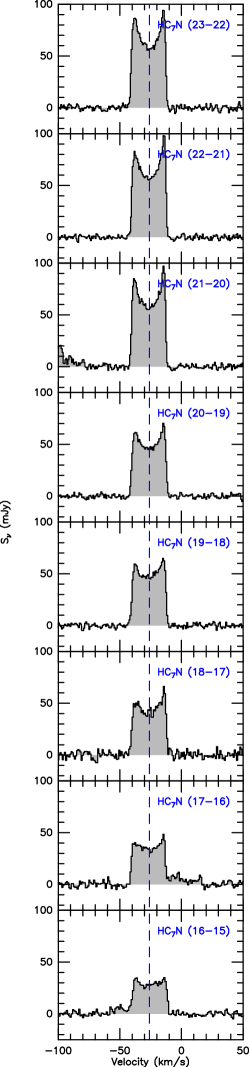
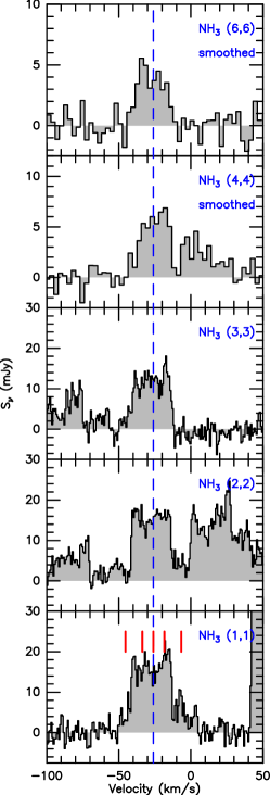
Figure 2: Detected spectra of HC₇N and NH₃ with transitions marked in the upper right of each panel. The NH₃ (4,4) and (6,6) lines have been smoothed to have a channel width of $\sim$3.3 km s^-1, while the channel width of other lines is $\sim$0.8 km s^-1. In the NH₃ (1,1) panel, the positions of the satellites are indicated by red solid lines. The blue dashed line traces the systemic LSR velocity ($-$26.0 km s^-1) of IRC +10216.

HC₇N. – Eight transitions of HC₇N from $J=16-15$ to $J=23-22$ fall in our band and are all detected. From Fig. 2, their line intensities rise with increasing frequency. Furthermore, we find that higher $J$ transitions have deeper dips than lower $J$ transitions in the center of line profiles. This is because the higher angular resolution of the higher $J$ transitions ends up lowering the contribution of emission from the CSE’s outer regions to the line profiles. Apparently, the possible decrease in source size owing to higher excitation requirements of higher $J$ lines is less pronounced than effects caused by the decreasing beam size. HC₇N (21–20) has been reported before (Winnewisser & Walmsley 1978), but the peak intensity also obtained for it with the 100-m telescope is almost twice the peak intensity measured by us.

HC₉N. – There are 14 transitions of HC₉N in our band. Five of them have been reported before (Bell et al. 1992; Truong-Bach et al. 1993). The intensity of HC₉N (43–42) measured by us is roughly twice the intensity reported, also from Effelsberg, by Truong-Bach et al. (1993).

SiC₄. – There are three lines of SiC₄ in this band and two of them are detected. They have lower upper level energies than previously reported transitions that span a frequency range from $\sim 30$ to $\sim 100$ GHz (Kawaguchi et al. 1995; Mauersberger et al. 2004). Although SiC₄ ($6$–$5$) falls into our frequency range as well, it is apparently too weak and remained undetected. This is consistent with the fact that the $J$=$7$–$6$ line is found to be significantly weaker than the $J$=$8$–$7$ line.

NH₃. – We measured the five metastable inversion transitions ($J$, $K$) = (1,1), (2,2), (3,3), (4,4), (6,6) of ammonia (NH₃). The (5,5) line, also inside the measured band, is not seen (the non-detection of NH₃ (5,5) is discussed in Sect. 4.3). NH₃ (1,1) and NH₃ (2,2) have been reported by Nguyen-Q-Rieu et al. (1984) with the 100-m telescope, and their peak intensities are similar to ours. Inspecting Fig. 2 and Table LABEL:Tab:irclines, we find that the metastable inversion lines become slightly narrower with increasing $J$. Furthermore, we do not find clear evidence for hfs components in the NH₃ lines. For example, the (1,1) transition has one main and four satellite groups of hfs components, the centroid velocities of the groups of hfs components are symmetrically spaced by $\approx\pm 7.6$ km s^-1  and $\pm 19.4$ km s^-1  from the main group (Kukolich 1967). Had the satellite groups appreciable optical depths this would lead to a significant (and symmetrical) broadening of this line. Assuming that all components of NH₃ (1,1) have the same excitation temperature, the limits on integrated intensity ratios ($>$8) between the main component and the hyperfine structure components indicate that the optical depth of NH₃ (1,1) is very low and might even depart from local thermodynamic equilibrium (LTE ratios on the order of 4). Meanwhile, there are no non-metastable NH₃ lines ($J$$>$$K$) detected. Non-metastable NH₃ lines require extreme densities (spontaneous radiative decay for rotational lines is $\sim 10^{5}$ times faster than for pure inversion transitions) or radiation fields to get excited and thus should only originate in the innermost shell. Any emission from this region would suffer from significant beam dilution effects.

MgNC. – The radical’s higher $J$ transitions have already been studied before (Kawaguchi et al. 1995; Guelin et al. 1993). This confirms our assignment about the $N$=2–1, $J$=5/2–3/2 transition of MgNC at 23875.0 MHz while the $N$=2–1, $J$=3/2–1/2 transition, also located within our frequency range, remains undetected. This is expected, since its integrated intensity may be $\sim$90 mJy km s^-1  (corresponding to a peak intensity of 3 mJy assuming an expansion velocity of 14 km s^-1  and a flat-topped line profile) according to the expected intensity ratio between $N$=2–1, $J$=5/2–3/2 and $N$=2-1, $J$=3/2–1/2 lines under conditions of LTE and optically thin emission (see Sect. 4) and there are large uncertainties related to weak transitions.

l-C₅H. – Five lines are detected in this survey, and they are from both the ${}^{2}\Pi_{1/2}$ and ${}^{2}\Pi_{3/2}$ ladders. Transitions of l-C₅H at higher frequencies have already been reported from IRC +10216 (Kawaguchi et al. 1995; Cernicharo et al. 1986).

C₆H. – The first identification of the C₆H radical toward IRC +10216 has been reported by Guelin et al. (1987). Six lines of C₆H are observed here, stemming from both the ${}^{2}\Pi_{1/2}$ and the ${}^{2}\Pi_{3/2}$ ladders.

C₆H^-. – C₆H^- was the first detected interstellar anion, and its identification has been confirmed by observations toward IRC +10216 and TMC-1 (McCarthy et al. 2006). Three transitions of C₆H^- fall into our band, and two of them are detected. C₆H^- (7–6) is also inside the frequency range covered by this survey, but is expected to be weaker than C₆H^- (8–7).

C₈H. – C₈H is the longest C_2nH molecule detected so far. It was first discovered toward IRC +10216 by Cernicharo & Guelin (1996). Four lines of C₈H are detected in this survey, all from the ${}^{2}\Pi_{3/2}$ ladder. Their hfs is not resolved. C₈H $J$=39/2–37/2 has been detected in IRC +10216 by Remijan et al. (2007), and the intensity agrees well with our measurement.

3.3 Unidentified lines

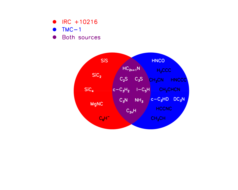
Figure 7: Schematic diagram of detected molecules in the same $\lambda\sim$ 1.3 cm spectral range toward IRC +10216 and TMC-1. Molecules in the red, blue, and purple regions indicate that they are detected in IRC +10216, TMC-1, and both sources, respectively. The molecules in black indicate that they have been seen in both sources but are not detected toward the other source in the $\lambda\sim$ 1.3 cm spectral range (see Sect. 4.5).

We do not see the 22.2 GHz line of water vapor (see Melnick et al. 2001; Cherchneff 2011; Neufeld et al. 2011, 2013, for detections of higher frequency transitions). This may be due to a coherent gain path of insufficient length or incorrect density-temperature combinations. For the 22.2 GHz line to mase, $T_{\rm kin}\sim$ 400 K and $10^{8}\leavevmode\nobreak\ \rm{cm^{-3}}<n<10^{9}\leavevmode\nobreak\ \rm{cm^{-3}}$ may be required (e.g., Kylafis & Norman 1991). This could be met in the inner envelope. If the density were too high in the $T\sim$ 400 K region, the maser action would be quenched. However, in that case, thermal emission would be expected. Assuming optically thick emission at $T_{\rm kin}=$ 600 K for the 22.2 GHz line and an emitting region of ten stellar radii or 0.8″  (roughly consistent with the $T_{\rm kin}$-radius profile in Fig. 7 of Crosas & Menten 1997), we get in our 43″ beam (Sect. 2) $T_{\rm mb}$ = 600$\times$ 10³ $\times$ (1.6/43)² mK, which gives an approximate $T_{\rm mb}\sim$ 800 mK. We clearly do not see this at a 5 $\sigma$ noise level of $T_{\rm mb}\sim$ 10 mK and conclude that the assumption of optically thick emission must be incorrect. This is consistent (E. Gonzalez-Alfonson, priv. comm) with the model that reproduces the H₂O data from Herschel, published by Neufeld et al. (2011). The C₅S lines are also not seen in our K-band spectral range (see Agúndez et al. 2014, for a report about the discovery of C₅S in IRC +10216) while Bell et al. (1993a) claimed detecting one C₅S line at 23990.2 MHz with a peak flux density of almost 20 mJy. With expected rotational temperatures of $18-44$ K and expected column densities of $(2-14)\times 10^{12}$ cm^-2 (Agúndez et al. 2014), we can estimate the peak intensity of the C₅S 23990.2 MHz line by assuming a low opacity, a flat-topped line profile, an expansion velocity of 14 km s^-1, a source size of 30″  and a beamsize of 40″. The derived peak intensity is estimated to be $0.3-4$ mJy, corresponding to an integrated intensity of 8.4–112 mJy km s^-1, where its electric dipole moment is taken to be 5.12 D (Botschwina 2003). Thus, our non-detection of the C₅S lines is expected and the detection reported by Bell et al. (1993a) remains unconfirmed.

When referring to detected spectral features, we find 12 unidentified lines in this survey that cannot be assigned to any transitions in the spectroscopic catalogs available to us. Their high percentage ($\sim$15% of the total number of lines) is probably due to the high sensitivity of the survey since their peak intensities are all less than 10 mJy. All of them show U-shaped or flat-topped profiles so they may represent isotopologues of well-known molecules or vibrationally excited lines or new species, and are marked with “U” in Table LABEL:Tab:irclines. The frequencies of unidentified lines are determined by eye assuming a source velocity of $V_{\rm lsr}=-$26.0 km s^-1. The accuracy of the frequencies of the U lines is estimated to lie within $\sim$180 kHz which is equivalent to three raw channels. The “U” line at 24901.4 MHz is close to C₄H (${}^{2}\Pi_{1/2}$) ($\nu_{7}=1$, $J=5/2-3/2$, $l=e$), and their frequency difference is 454 kHz, corresponding to $\sim$5.5 km s^-1. Another “U” line at 25111.8 MHz is close to CH₂CHCN (10_1,9–10_1,10) with a rest frequency at 25111.4 MHz, but this line as observed would not be expected from this molecule because its fitted expansion velocity is about 19 km s^-1, if we use a single component to fit it. This is higher than the typical expansion velocity deduced from other detected transitions of CH₂CHCN in IRC +10216 (Agúndez et al. 2008). Furthermore, the integrated intensity of CH₂CHCN (10_1,9–10_1,10) is expected to be around 0.3 mJy km s^-1  under the LTE assumption and assuming the column density and rotational temperature determined by Agúndez et al. (2008) , which is much less than that of this “U” line.

Among the “U” lines, we find that there are three doublets, at 22304.854 MHz and 22323.3 MHz (pair-1, 18.5 MHz apart), at 25094.3 MHz and 25111.8 MHz (pair-2, 17.5 MHz apart), and at 25976.2 MHz and 25992.8 MHz (pair-3, 16.6 MHz apart). Their separations (16 MHz to 19 MHz) could be caused by hfs or different ¹³C substitutions. Estimates of their carrier’s rotational constant ($B$) and centrifugal stretching constant ($D$) can help to make guesses about their identity. Assuming that two or three of them are from the same linear molecule, $B$ and $D$ can be derived via the formula (Wilson et al. 2009)

$$\nu(J)=2B(J+1)-4D(J+1)^{3},$$ (1)

where $\nu$ is the rest frequency of the $J$ – ($J-1$) transition. We follow two steps to fit the parameters $B$ and $D$. Firstly, we obtain the number of $J$ with $D=0$. $J$ has to be an integer. Secondly, $B$ and $D$ can be derived with $J$ fixed. We find that the three doublets cannot be attributed to one species. If they belonged to one species, the three doublets would have to be assigned to the $J$, $J+3$, and $J+4$ levels but the $J+1$ and $J+2$ levels are not detected in our band. Furthermore, the fitted $D$ would be negative. Thus, we assume that two of them belong to the $J$ and $J+1$ levels of one species to derive the parameters $J$, $B$, and $D$. Since $D$ is usually a very small number, results are dismissed when the derived $D$ is larger than 0.5 MHz. The results are given in Table. 2.

We find that the derived rotational constants are very small, which indicates a heavy molecule. When we assume that pair-1 and pair-2 come from the same species, the derived rotational constants are similar to that (1391.2 MHz) of C₆H. We note, however, that these rotational constants allow us to predict additional lower $J$ lines within our surveyed frequency range, which are not seen. It is probably because the lower $J$ level transitions are weaker than higher ones and cannot be detected by this survey.

4 Discussion

4.1 Rotational temperatures and column densities

Line shapes can be used to evaluate the optical depth of individual transitions in IRC +10216. Parabolic lines arise from optically thick emission like that of CO (1–0), while flat-topped and U-shaped lines arise from optically thin spatially unresolved and resolved emission, respectively (Olofsson et al. 1982; Kahane et al. 1988). We find no lines that show parabolic profiles among the identified spectral features in this survey. Also, lines with hfs should allow for estimates of their optical depth, if the hfs components are sufficiently displaced from each other (see the case of NH₃ discussed above). For such lines in our survey (NH₃, HC₃N, C₃N, etc.), we find low opacities. Thus, it is reasonable to assume optically thin emission for all the lines detected in this work. Assuming LTE, we use rotational diagrams to roughly estimate rotational temperatures and column densities. The standard formula used here is

$${\rm ln}(\frac{3kW}{8\pi^{3}\nu\mu^{2}S})\leavevmode\nobreak\ =\leavevmode\nobreak\ {\rm ln}(\frac{N_{\rm tot}}{Q(T_{\rm rot})})-\frac{E_{\rm u}}{kT_{\rm rot}},$$ (2)

where $k$ is the Boltzmann constant, $W$ the integrated intensity, $S$ the transition’s intrinsic strength, $\mu$ the permanent dipole moment, $N_{\rm tot}$ the total column density, $T_{\rm rot}$ the rotational temperature, $Q$ the partition function, and $E_{\rm u}$ the upper level energy of the transition. The values of $Q$ and $\mu$ are taken from the CDMS and JPL catalogs.

At least two transitions of the same molecule with significant energy differences are required to determine rotational temperatures with this method. For those molecules with only one transition detected or without a wide dynamic range in upper level energies, we make use of the 28 GHz to 50 GHz data from Kawaguchi et al. (1995), the C₈H data from Remijan et al. (2007), and the C₃N data from He et al. (2008), because those data have nearly the same resolution ($\sim 40$″) as our observations. The intensities of blended lines have large uncertainties, so are not included. SiS is also excluded, since SiS (1–0) is a maser in IRC +10216 (Grasshoff et al. 1981; Henkel et al. 1983) and the populations must deviate from LTE.

To derive the physical parameters, the intensities should be corrected for beam dilution by dividing by $\theta_{\rm s}^{2}/(\theta_{\rm s}^{2}+\theta_{\rm beam}^{2})$, where $\theta_{\rm s}$ is the source size, and $\theta_{\rm beam}$ is the beam size. Based on previous high resolution mapping of different molecules toward IRC +10216, we take the same source sizes as those listed in Table 3. For species without high resolution mapping, their sizes are taken to be the same as chemically related species (details are described in the notes of Table 3). We also used different source sizes $\theta_{\rm s}=15\arcsec,18\arcsec,30\arcsec,50\arcsec$ to study the influence on the derived rotational temperatures and column densities of these molecules. It turns out that the uncertainties of the total column densities vary within a factor of four while the rotational temperatures nearly remain the same.

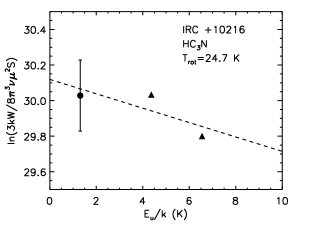
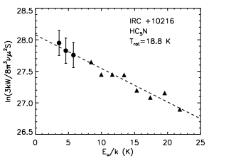
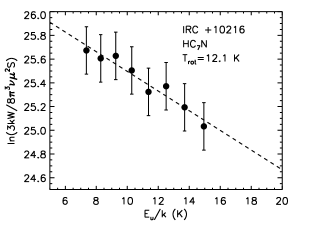
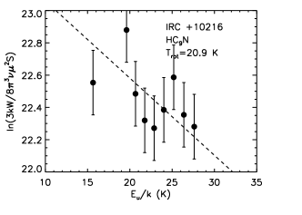
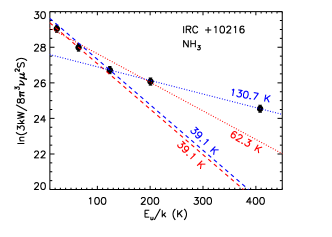
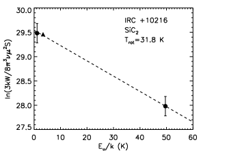
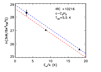
Figure 3: Rotational diagrams for the observed molecules in IRC +10216. For lines with hfs, all observed components have been taken into account. The circles with error bars are from our Effelsberg-100 m observations, where in addition to uncertainties in the fit to the integrated line intensities, a calibration error of 20% has also been included. Filled and open symbols indicate signal-to-noise ratios that are larger than or less than five, respectively. The triangles without error bars are obtained from Kawaguchi et al. (1995). The pentagrams with error bars for C₈H are obtained from Remijan et al. (2007), and the squares for C₃N are from He et al. (2008). Their values have been corrected for beam dilution. The molecules and their corresponding rotational temperatures, obtained from unweighted linear fits, are given in the upper right corner of each panel. Black dashed lines represent linear least-squares fit to the rotational diagram accounting for data presented by filled symbols, and the black dot-dashed lines represent the fit when the open circles are included. The red and blue dashed lines represent fits for the para and ortho states of NH₃ and c-C₃H₂ and the ${}^{2}\Pi_{1/2}$ and ${}^{2}\Pi_{1/2}$ state of l-C₅H and C₆H, respectively. Specifically for NH₃, the red dashed line shows the fit to the ($J,K$) = (1,1) and (2,2) para-lines, the blue dashed line uses the resulting excitation temperature (39.1 K) and the ortho-(3,3) line, the dotted red line represents a fit to the para-(1,1), (2,2), and (4,4) transitions and the blue dotted line fits the ortho-(3,3) and (6,6) transitions.

We carried out linear least-square fits to the rotational diagrams of 17 species and four ¹³C isotopologues of HC₅N, which are shown in Fig. 3. For these fits, only data with signal-to-noise ratios higher than five are taken. The figures show that a few lines from the literature are outliers. In particular, SiC₄ (16–15) at $E_{\rm u}/k$= 20.0 K is much weaker than expected, and the data of C₆H (${}^{2}\Pi_{3/2}$) from Kawaguchi et al. (1995) show significant scatter. This is due to weak lines with signal-to-noise ratios less than five, which, as mentioned above, have not been included in the fits. Therefore, only data points with higher signal-to-noise ratios than five are taken into account if there are enough points for the fits. Otherwise, data points with lower signal-to-noise ratios are also included and the fit to the data is represented not by a dashed but by a dash-dotted line. For example, those data points with signal-to-noise ratios less than five are used for the fits of ¹³C isotopologues of HC₅N and C₈H. The quality of the calibration of our observations is indicated by the fact that the data points for the HC₇N transitions show very little scatter about the fitted line in Fig. 3, while their frequencies cover nearly the entire frequency range surveyed by us. For l-C₅H (${}^{2}\Pi_{3/2}$), we only detect one line that cannot be fitted with the data from Kawaguchi et al. (1995), because this would result in a negative excitation temperature. We therefore use the rotational temperature derived from their data and our measured transition to obtain its column density (see the lower dashed line in the respective panel of Fig. 3; the upper dashed line refers solely to the data of Kawaguchi et al. 1995).

HC₉N shows large scatter, which may result from uncertainties related to its low line intensities. The HC₉N transitions from Kawaguchi et al. (1995) are not included since they show an even larger scatter. For NH₃ and c-C₃H₂, we fit their para and ortho states individually. If we only take NH₃ (1,1), (2,2), and (3,3) into account, the ortho/para ratio of NH₃ is estimated to be 1.3$\pm$0.6 in IRC +10216, which roughly agrees with the fact that the ortho/para abundance ratio approaches the statistical ratio of unity if NH₃ was formed in a medium with a kinetic temperature higher than $\sim$40 K (Takano et al. 2002). Including the NH₃ (4,4) and NH₃ (6,6) lines yields a higher rotational temperature and a lower ortho column density (see Table 3). The ortho/para abundance ratio then becomes $0.6\pm 0.2$. The derived ortho/para ratio of c-C₃H₂ is about 1.4$\pm$0.3, which is much less than the expected theoretical value of 3. We only have two points to fit the rotational temperature, and para and ortho $T_{\rm rot}$ values are assumed to be the same. We also fit the ${}^{2}\Pi_{1/2}$ and ${}^{2}\Pi_{3/2}$ states, separately, for l-C₅H and C₆H. However, the fits for l-C₅H (${}^{2}\Pi_{3/2}$) shown in Fig. 3 are tentative and should have large uncertainties because the data used here have an energy range ($\Delta E/k$) less than 10 K.

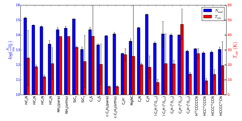
Figure 4: Comparison of the column densities and rotational temperatures of different molecules. The labels for column densities are blue on the left side, while those for rotational temperatures are red on the right side. Here, a $T_{\rm rot}$ of 39.1 K has been taken for para and ortho NH₃ (see Sect. 4.1 and Table 3)

The derived rotational temperatures ($T_{\rm rot}$) and column densities ($N$), together with results from the literature, are listed in Table 3. MgNC and C₂S show the largest uncertainties in the rotational temperature, which is due to the narrow energy ranges covered. From Table 3, we find that the derived column densities agree roughly with previous studies. From Fig. 4, taking $T_{\rm rot}=39.1\pm 10.5$ K for the bulk of the para and ortho NH₃, we find rotational temperatures ranging from 5.5 to 47.2 K and molecular column densities ranging from 5.2$\times 10^{12}$ to 2.4$\times 10^{15}$ cm^-2. C₆H (${}^{2}\Pi_{3/2}$) has the highest rotational temperature, while c-C₃H₂ has the lowest rotational temperatures indicating that they should be present in the cold outer molecular envelope. C₄H, SiC₂ and HC₃N are found to be the most abundant carbon-bearing molecules in our survey while C₆H^-, C₈H, and the ¹³C substitutions of HC₅N have the lowest column densities (see Table 3). The column densities of all these species are spread over two orders of magnitude, and more complex molecules tend to be less abundant.

4.2 Fractional abundances relative to H₂

To obtain molecular abundances relative to H₂, one has to know the H₂ column density. Kendall et al. (2002) employed optical absorption spectroscopy toward background stars lying behind the envelope and found that the H+2H₂ column density at an offset of 37″ from IRC +10216 is $\sim$2$\times 10^{21}$ cm^-2. Based on the optically thin lines of ¹³CO (1–0), (2–1), and (3–2), Groesbeck et al. (1994) determined a beam-averaged ($\sim$20″) CO column density of $\sim$2$\times 10^{18}$ cm^-2 toward IRC +10216 by taking ¹²C/¹³C to be 44. Previous studies have shown the fractional abundance CO/H₂ to be $6\times 10^{-4}$ in IRC +10216 (Kwan & Linke 1982; Huggins et al. 1988), resulting in an H₂ column density of 3.3$\times 10^{21}$ cm^-2. Furthermore, the average H₂ column density can also be calculated from the mass loss rate via the formula

$$N_{\rm H_{2}}=\frac{\dot{M}R/V_{\rm exp}}{\pi R^{2}m_{\rm H_{2}}}=\frac{\dot{M}}{\pi RV_{\rm exp}\,\mu m_{\rm H}}\leavevmode\nobreak\ ,$$ (3)

where $\dot{M}$ is the mass loss rate which is believed to be 2.0$\times 10^{-5}M_{\odot}$yr^-1 (Crosas & Menten 1997); $R$ is the radius; $V_{\rm exp}$ is the expansion velocity of the CSE which is equal to 14 km s^-1; $\mu$ is the mean molecular weight, which we assume to be equal to 2.8; and $m_{\rm H}$ is the mass of a hydrogen atom. Of course, reference H₂ column densities to be used for abundance calculations depend on the location of their emission region in the CSE (see Formula 3). For example, if we take $R$ as the CO radius (100″; Fong et al. 2006) and the HC₃N radius of 15″(Table 3), the H₂ average column densities inside these radii are 3.2$\times 10^{20}$ cm^-2 and 2.1$\times 10^{21}$ cm^-2, respectively. While each line has a different distribution and therefore an individual $N_{\rm H_{2}}$, the choice of a specific $N_{\rm H_{2}}$ for all molecules is needed for a meaningful comparison with other studies. Thus, we use the H₂ average column density (2.1$\times 10^{21}$ cm^-2) within a typical radius of 15″ to calculate molecular fractional abundances relative to H₂. The uncertainty of the average H₂ column density is within a factor of two since most detected molecules have a characteristic radius ranging from 7.5″  to 30″  in IRC +10216. The results are given in the fourth column of Table 3. We find the fractional abundances relative to H₂ range for K-band detected species from 2.5$\times$10^-9 to $1.1\times$10^-6 in IRC +10216.

4.3 The RADEX non-LTE modeling for NH₃: the kinetic temperature

Here we present a non-LTE analysis of NH₃ to determine the envelope’s kinetic temperature using the RADEX expanding sphere code for IRC +10216 (van der Tak et al. 2007). NH₃ is well suited to temperature determinations even with the limited frequency range covered by our survey, since its transitions arise from a wide range of energies above the ground state. Moreover, the metastable inversion lines are widely used as a galactic and extragalactic molecular temperature tracer (e.g., Walmsley & Ungerechts 1983; Ho & Townes 1983; Mauersberger et al. 2003).

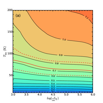
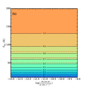
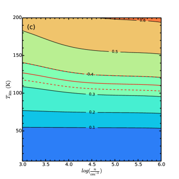
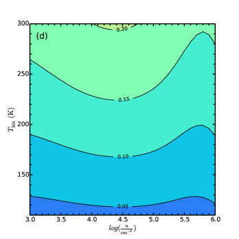
Figure 5: RADEX non-LTE modeling for NH₃. (a) the integrated intensity ratio $\frac{\rm NH_{3}(2,2)}{\rm NH_{3}(1,1)}$ as a function of $n_{\rm H_{2}}$ and $T_{\rm kin}$ for a given para-NH₃ abundance per velocity gradient [X]/(d$v$/d$r$) of $4.4\times 10^{-11}$ pc (km s^-1)^-1. (b) the integrated intensity ratio $\frac{\rm NH_{3}(2,2)}{\rm NH_{3}(1,1)}$ as a function of [X]/(d$v$/d$r$) and $T_{\rm kin}$ for a given density of 10⁵ cm^-3. In both panels, the levels go from 0.1 to 1 by 0.1. (c) the integrated intensity ratio $\frac{\rm NH_{3}(4,4)}{\rm NH_{3}(2,2)}$ as a function of $n_{\rm H_{2}}$ and $T_{\rm kin}$ for a given para-NH₃ abundance per velocity gradient [X]/(d$v$/d$r$) of $4.4\times 10^{-11}$ pc (km s^-1)^-1. The levels start from 0.1 to 0.6 by 0.1. The red solid line and the dashed lines represent the observed line ratio as well as its lower and upper limit in Fig. 5a, b and c. (d) the integrated intensity ratio $\frac{\rm NH_{3}(6,6)}{\rm NH_{3}(3,3)}$ and as a function of $n_{\rm H_{2}}$ and $T_{\rm kin}$ for a given ortho-NH₃ abundance per velocity gradient [X]/(d$v$/d$r$) of $5.6\times 10^{-11}$ pc (km s^-1)^-1. The levels start from 0.05 to 0.2 by 0.05. The observed line ratio $\frac{\rm NH_{3}(6,6)}{\rm NH_{3}(3,3)}$ = (0.28$\pm$0.08) is beyond the modeled range, indicating that the kinetic temperature is either higher than 300 K or that NH₃ (6,6) is affected by population inversion.

Assuming that NH₃ has a typical expanding velocity of 14 km s^-1and a size of 18″ (see Sect. 4.1), we obtain a velocity gradient of about 2468 km s^-1 pc^-1. Adopting a fixed para-NH₃ abundance of 1.1$\times 10^{-7}$ (see Table 3 and, for chemical considerations, Menten et al. (2010)) and a velocity gradient of 2500 km s^-1 pc^-1, we arrive at a para-NH₃ abundance per velocity gradient $[X]/(dv/dr)$ of $4.4\times 10^{-11}$ pc (km s^-1)^-1. The modeled kinetic temperatures range from 10 to 300 K with a step size of 5 K. The H₂ number density log($\frac{n(\rm{H}_{2})}{\rm cm^{-3}}$) varies from 2.0 to 7.0 with a step size of 0.1. For an adopted size of the NH₃ region of 18″, the density is around 10⁵ cm^-3 according to the density profile toward IRC +10216 (Groenewegen et al. 1997). We modeled the integrated intensity ratios $\frac{\rm NH_{3}(2,2)}{\rm NH_{3}(1,1)}$ in this study, which are shown in Fig. 5a, because (a) the ratio between NH₃ (1,1) and NH₃ (2,2) is not affected by an ortho-to-para abundance ratio, because (b) NH₃ rotation temperatures provide lower limits to the kinetic temperature (e.g., Walmsley & Ungerechts 1983) with the ($J$,$K$) = (1,1), (2,2), and (3,3) transitions revealing the lowest $T_{\rm rot}$ values, and because (c) beam-filling factors (the (1,1) and (2,2) frequencies are less than 30 MHz apart) should not play a role. Assuming that both lines arise from the same source, we obtain a kinetic temperature of 70$\pm$20 K for NH₃ in the density range from $10^{4.5}$ to $10^{5.5}$ cm^-3 with an integrated intensity ratio $\frac{\rm NH_{3}(2,2)}{\rm NH_{3}(1,1)}$ of $0.73\pm 0.1$ (see Fig. 5a).

The value of the para-NH₃ abundance per velocity gradient $[X]/(dv/dr)$, which was given at the start of the previous paragraph, may have a large uncertainty, potentially also leading to a significant error bar in our $T_{\rm kin}$ estimate. Thus, we carried out a non-LTE analysis with a fixed density of $10^{5}$ cm^-3 (see previous paragraph) and the para-NH₃ abundance per velocity gradient $[X]/(dv/dr)$ ranging from $1.0\times 10^{-13}$ to $1.0\times 10^{-9}$ pc (km s^-1)^-1. The result is shown in Fig. 5b. We find that the kinetic temperature does not depend on the para-NH₃ abundance per velocity gradient $[X]/(dv/dr)$ in the range of 10^-13 to 10^-9 pc (km s^-1)^-1, because the lines are optically thin. Therefore, the kinetic temperature of 70$\pm$20 K derived from the integrated intensity ratio $\frac{\rm NH_{3}(2,2)}{\rm NH_{3}(1,1)}$ is reasonable for the NH₃ environment in IRC +10216.

At the same time, we also modeled the integrated intensity ratios $\frac{\rm NH_{3}(4,4)}{\rm NH_{3}(2,2)}$ and $\frac{\rm NH_{3}(6,6)}{\rm NH_{3}(3,3)}$ (see Figs. 5c and 5d). While modeling the integrated intensity ratios $\frac{\rm NH_{3}(6,6)}{\rm NH_{3}(3,3)}$, an ortho-NH₃ abundance per velocity gradient $[X]/(dv/dr)$ of $5.6\times 10^{-11}$ pc (km s^-1)^-1 is used with the same velocity gradient as for para-NH₃. With the observed integrated intensity ratio $\frac{\rm NH_{3}(4,4)}{\rm NH_{3}(2,2)}=(0.36\pm 0.04)$ and the assumption that NH₃ (2,2) and (4,4) arise from the same region, we obtain a kinetic temperature of 120${}^{+10}_{-5}$ K in the density range from $10^{4.5}$ to $10^{5.5}$ cm^-3. We note that NH₃ (4,4) might be blended (see Fig. 9) by a feature of unknown origin, in which case the derived kinetic temperature would be slightly overestimated. In any case, the derived kinetic temperature is higher than obtained from the observed integrated intensity ratio $\frac{\rm NH_{3}(2,2)}{\rm NH_{3}(1,1)}$, which indicates a kinetic temperature gradient with NH₃ (4,4) originating in a warmer region.

For ortho-NH₃, the observed line ratio $\frac{\rm NH_{3}(6,6)}{\rm NH_{3}(3,3)}$ = (0.28$\pm$0.08) is beyond the modeled range, which indicates that NH₃ (6,6) may arise from a very hot region with a kinetic temperature larger than 300 K. Alternatively, the (6,6) emission may be affected by population inversion and an optical depth not far below unity. Such NH₃ (6,6) masers have already been found in NGC 6334I (Beuther et al. 2007), W51–IRS2 (Henkel et al. 2013), and perhaps even in the nearby galaxy IC 342 (Lebrón et al. 2011), all of which are sources where a strong infrared radiation field may significantly contribute to the molecule’s excitation. The inner parts of IRC+10216’s envelope also possess this strong a radiation field. On the other hand, NH₃ (5,5) is not detected in this survey. Adopting $T_{\rm rot}$= 62.3 K from a fit to the (1,1), (2,2), and (4,4) para-NH₃ lines, the integrated intensity of NH₃ (5,5) is predicted to be 35 mJy km s^-1 , which is too weak to be detected. The non-detection of the (5,5) and (7,7) lines does not provide evidence for NH₃ formation pumping, which has recently been suggested for a variety of molecules in star-forming regions (Lis et al. (2014), see also Wilson et al. (2006) for a particularly compelling observational candidate).

4.4 Abundance differences among ¹³C isotopologues of HC₅N and the ¹²C/¹³C ratio in IRC +10216

Chemical fractionation of ¹³C-bearing species has been observed toward low-temperature regions. Takano et al. (1998) reported chemical fractionation between the ¹³C isotopologues of HC₃N toward TMC-1. Sakai et al. (2007) report a C¹³CS/¹³CCS ratio of 4.2$\pm$2.3 (3$\sigma$) in TMC-1. Sakai et al. (2010) also find the C¹³CH /¹³CCH abundance ratios to be 1.6$\pm$0.4 (3$\sigma$) and 1.6$\pm$0.1 (3$\sigma$) for TMC-1 and L1527. Finally, Sakai et al. (2013) find abundance differences among ¹³C isotopologues of C₃S and C₄H in TMC-1, which are believed to be caused by different formation processes or ¹³C isotope exchange reactions. However, in IRC +10216, ¹³C isotope fractionation is still not very well studied.

In our band, the ¹³C isotopologues of HC₃N, HC₅N, C₂S, C₃S, and C₄H can be used to address this issue. However, H¹³CCCN (2–1) at 17633.7 MHz lies outside of our frequency range. The bands related to the (2–1) transition of HC¹³CCN and HCC¹³CN at 18120.8 MHz and 18119.0 MHz are flagged. Meanwhile, the ¹³C isotopologues of C₂S, C₃S, and C₄H are too weak to be detected in this survey. However, many of the ¹³C-bearing isotopologues of HC₅N have been measured (see Sect. 3.2) and are thus used to investigate potential abundance differences among the ¹³C species toward IRC +10216. The $J$=9–8 transitions of the ¹³C-bearing isotopologues are the strongest in our band, so we compare their integrated intensities, except for HC¹³CCCCN ($9-8$), which is blended with C₆H at 23719.4 MHz. With the four other $J$=9–8 transitions, the integrated line intensity ratios, applying a factor $\nu^{2}$ correction between H¹³CCCCCN, HCC¹³CCCN, HCCC¹³CCN, and HCCCC¹³CN, are estimated to be 1.00:(1.07$\pm$0.08):(1.28$\pm$0.09):(1.02$\pm$0.07). The errors represent 1$\sigma$. Therefore, the results suggest that the abundances of the ¹³C isotopologues of HC₅N may not be all the same in IRC +10216. He et al. (2008) may also have found an abundance differentiation among the ¹³C isotopologues of HC₃N in IRC +10216 by obtaining the integrated line intensity ratios H¹³CCCN:HC¹³CCN:HCC¹³CN=1.00:(1.19$\pm$0.14):(1.31$\pm$0.15), applying mm-wave spectroscopy. Thus, we suggest that abundance differences possibly exist between the ¹³C isotopologues of HC₅N, but this has to be further checked by deeper integrations.

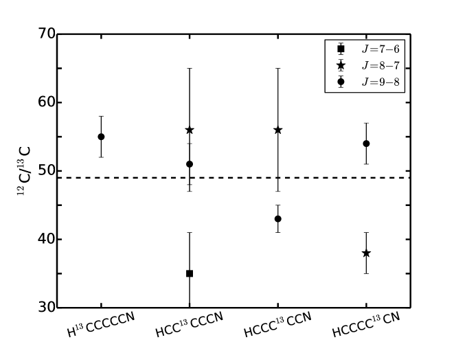
Figure 6: ¹²C/¹³C isotopic abundance ratios from HC₅N. The ratios are based on the integrated intensity of the transitions of HC₅N and its ¹³C isotopologues. The ratios derived from the $J$=7–6, $J$=8–7, and $J$=9–8 transitions are denoted with filled squares, pentagrams, and circles, respectively. The dashed line denotes the unweighted average ¹²C/¹³C value.

The ¹²C/¹³C ratio is an important tool for tracing processes of stellar nucleosynthesis (Wilson & Rood 1994). Here the carbon isotope ratio is based on the ratios between the same $J$ transitions from HC₅N and its ¹³C isotopologues. (The blended lines are not included.) The transitions of HC₅N and its ¹³C substitutions are optically thin as mentioned in Sect. 4.1. Thus, the isotopic ratio can be directly obtained from their integrated intensity ratio. Figure 6 shows the ¹²C/¹³C ratios determined with eight pairs of unblended transitions from HC₅N and its ¹³C isotopologues. The derived ¹²C/¹³C ratios are $35\pm 6$ from $J=7-6$, $56\pm 9$, $56\pm 9$, and $38\pm 3$ from $J$=8–7, and $55\pm 3$, $51\pm 3$, $43\pm 2$, and $54\pm 3$ from $J=9-8$. The unweighted average ¹²C/¹³C ratio is $49\pm 9$, where the error is the standard deviation of the mean. This is greater than was derived from [SiCC]/[Si¹³CC] ($34.7\pm 4.3$) by He et al. (2008) and less than the 71 obtained from [¹²CO]/[¹³CO] by Ramstedt & Olofsson (2014), but these results may suffer from opacity effects. Our value agrees well with the 47${}^{+6}_{-5}$ of Kahane et al. (1988) derived from HC₃N, CS, HNC, CCH, SiCC, and their isotopologues. Therefore, we confirm that the ¹²C/¹³C ratio in IRC +10216 is much smaller than the terrestrial ratio (89) and is also smaller than the value found for the local interstellar medium ($\sim$70) (Wilson & Rood 1994).

4.5 Comparison of the IRC +10216 and TMC-1 chemistry

IRC +10216 and TMC-1, the dark cloud in the Taurus region, are the two prototypical sources for detailed studies of carbon chain molecules in outer space. Seen at distances of $D$ $\sim$ 130 pc (Sect. 1) and 140 pc (e.g., Pratap et al. 1997), respectively, they can be studied with similar linear resolution and sensitivity. Kaifu et al. (2004) carried out a line survey toward the cyanopolyyne peak of the dark cloud TMC-1 that includes the frequency range (17.8-26.3 GHz) discussed in this work. This allows us to compare chemical compositions between two physically different, prototypical astronomical environments characterized by large amounts of carbon chain molecules. We note that such a comparison may be biased by (1) the use of different telescopes, (2) by different source morphologies, and (3) by differences in line shapes, which all will affect relative sensitivities. While the TMC-1 study, carried out with the Nobeyama 45-m telescope, is characterized by a larger beam size, emission from TMC-1 is more extended than from IRC +10216, so that our Effelsberg 100-m data may actually suffer from smaller beam-filling factors. On the other hand, lines from IRC +10216, affected by an expansion velocity of $\sim$14 km s^-1, are much broader than those from TMC-1, thus allowing us to smooth contiguous channels and to compensate for this disadvantage. This implies that sensitivities match each other by a factor of a few. Below, we constrain ourselves mainly to K-band data, but referring also to lines from other spectral ranges if needed.

Comparing the detected molecules in the same $\lambda$ $\sim$1.3 cm spectral range (see Fig. 7), we find that five molecules are only detected in IRC +10216, nine molecules are only detected in TMC-1, and 13 molecules are detected in both sources. The five K-band molecules only detected in IRC +10216 are SiS, SiC₂, SiC₄, MgNC, and C₆H^-. While C₆H^- is not detected in the Nobeyama survey (Kaifu et al. 2004) toward TMC-1, it has been reported in later studies (e.g. McCarthy et al. 2006; Brünken et al. 2007). In contrast, MgCN could not be detected in a more recent sensitive study with the Green Bank 100-m telescope (Turner et al. 2005). This also holds for Si-bearing molecules (Ziurys et al. 1989). The nine K-band molecules only detected in TMC-1 are HNCO, HNCCC, CH₃CN, CH₂CHCN, c-C₃HD, HCCNC, CH₂CN, H₂CCC, and DC₃N. While HNCCC, CH₃CN, CH₂CHCN, HCCNC, CH₂CN, and H₂CCC are not detected in our survey, they have been reported by other studies (e.g., Gensheimer 1997; Agúndez et al. 2008; Cernicharo et al. 2000a). The other K-band molecules, HC_2n+1N (n = 1, 2, 3, 4), C_2nH (n = 2, 3, 4), c-C₃H₂, l-C₅H, C₃N, C₂S, C₃S, and NH₃, are detected in both sources which indicates, as already mentioned, that the two targets are both effective in forming long carbon-chain molecules. The ratio $\frac{\rm NH_{3}(2,2)}{\rm NH_{3}(1,1)}$ is less than 0.1 in TMC-1, indicating that the NH₃ emitting region in TMC-1 is much colder ($\sim$ 10 K) than in IRC +10216, consistent with its more pronounced deuteration of molecules. The cyanopolyyne abundance ratios are estimated to be HC₅N:HC₇N:HC₉N=(18.4$\pm$10.3):(14.8$\pm$8.4):1 in IRC +10216 while they are HC₅N:HC₇N:HC₉N=13.1:4.8:1 in TMC-1 (Sakai et al. 2008). The difference is probably related to different physical conditions or time scales for the formation and destruction of the cyanopolyynes in IRC +10216 and TMC-1. Meanwhile, there is no trend of the rotational temperatures of the cyanopolyynes increasing with the C-chain length that is found in TMC-1 (Bell et al. 1998). This indicates that the cyanopolyynes are probably emitting line photons from nearly the same region in IRC +10216. In IRC +10216, our C₆H^-/C₆H ratio is estimated to be (3.6$\pm$0.8)%. (The C₆H column density is the sum of the column densities of the ${}^{2}\Pi_{1/2}$ and the ${}^{2}\Pi_{3/2}$ states.) The value is lower than the 8.6%  derived in a previous study of IRC +10216 (Kasai et al. 2007), because they obtained a higher rotational temperature (33 K) for C₆H, resulting in a lower column density. To summarize, both C₆H^-/C₆H ratios in IRC +10216 are at least as high as the value (2.5%) reported for TMC-1 (McCarthy et al. 2006).

5 Summary and conclusions

We performed a 1.3 cm line survey toward IRC +10216 using the 100-m telescope at Effelsberg. In total, 78 spectral lines were detected, among which 12 remain unidentified. The identified lines are assigned to 18 different molecules and radicals. No new species was found, but 23 lines from already known species were detected for the first time outside the Solar System and there are an additional 20 lines first detected in IRC +10216. We also discuss the origin of the “U” lines.

Assuming LTE, we derived rotational temperatures and column densities of 17 detected molecules. Their rotational temperatures range from 5.5 to 39.1 K, and molecular column densities range from 5.2$\times 10^{12}$ to 2.4$\times 10^{15}$ cm^-2. Molecular abundances relative to H₂ range between 2.5$\times 10^{-9}$ and 1.1$\times 10^{-6}$. A non-LTE analysis of NH₃ shows that its (1,1) and (2,2) emission arises from the inner envelope with a kinetic temperature of 70$\pm$20 K, but there may be warmer gas as is indicated by the detected (4,4) line. The (6,6) inversion line shows surprisingly strong emission and might indicate inverted populations and an optical depth not far below unity. Comparing transitions from the ¹³C isotopologues of HC₅N, we find there might be abundance differences between them. The isotopic ¹²C/¹³C ratio is estimated to be 49$\pm$9 from the integrated intensity ratios of transitions from HC₅N and its ¹³C isotopologues. Finally, we compare the chemical compositions of IRC +10216 and TMC-1 in the $\lambda$ $\sim$1.3 cm spectral range. Apparently, Si-bearing molecules are favored in IRC +10216.

Table 2: Fitted results for the “U” line doublets.

$\nu(J-1)$	$\nu(J)$	$B$	$D$	$J$
(MHz)	(MHz)	(MHz)	($10^{-3}$MHz)
pair-1/pair-2
22304.9	25094.3	1395.605	3.101	8
pair-1/pair-3
22304.9	25976.2	1867.854	126.620	6
22323.3	25992.9	1870.374	140.234	6
pair-2/pair-3
25094.3	25976.2	451.506	2.164	28

Table 3: Column densities and rotational temperatures of the molecules in IRC +10216.

	This work						Other study
	$T_{\rm rot}$	$N$	X($N/N_{\rm H_{2}}$)	$\theta_{\rm s}$			$T_{\rm rot}$	$N$
Species	(K)	(cm-2 )		(″)	Note		(K)	(cm-2 )	Ref.
HC3N	24.7$\pm$18.5	$(1.4\pm 0.2)\times 10^{15}$	$6.7\times 10^{-7}$	30	1		28	$8.0\times 10^{14}$	10
							26	$1.7\times 10^{15}$	11
							12.7	$7.9\times 10^{14}$	14
HC5N	18.8$\pm$1.3	$(4.6\pm 0.2)\times 10^{14}$	$2.2\times 10^{-7}$	30	1		29	$2.3\times 10^{14}$	11
HC7N	12.1$\pm$1.3	$(3.7\pm 0.4)\times 10^{14}$	$1.8\times 10^{-7}$	30	2		26	$1.29\times 10^{14}$	11
HC9N	20.9$\pm$10.7	$(2.5\pm 1.4)\times 10^{13}$	$1.2\times 10^{-8}$	30	2		23	$2.7\times 10^{13}$	11
							12	$4.0\times 10^{13}$	17
NH3 (para)	39.1$\pm$10.5	$(2.3\pm 0.8)\times 10^{14}$	$1.1\times 10^{-7}$	18	3		133	$4.2\times 10^{13}$	20
NH3 (para)	62.3$\pm$5.9	$(2.7\pm 0.5)\times 10^{14}$	$1.3\times 10^{-7}$	18	3
NH3 (ortho)	39.1$\pm$10.5	$(2.9\pm 0.9)\times 10^{14}$	$1.4\times 10^{-7}$	18	3
NH3 (ortho)	130.7$\pm$17.0	$(1.5\pm 0.4)\times 10^{14}$	$7.1\times 10^{-8}$	18	3
SiC2	31.8$\pm$0.9	$(1.2\pm 0.0)\times 10^{15}$	$5.7\times 10^{-7}$	27	4		16	$2.2\times 10^{14}$	11
							96	$2.35\times 10^{15}$	10
							14	$9.5\times 10^{14}$	16
							60	$1.9\times 10^{15}$	16
SiC4	22.3$\pm$17.5	$(1.1\pm 0.4)\times 10^{13}$	$5.2\times 10^{-9}$	27	5		15	$7\times 10^{12}$	12
C2S	39.2$\pm$135.3	$(2.3\pm 0.8)\times 10^{14}$	$1.1\times 10^{-7}$	30	2		14	$1.5\times 10^{14}$	13
C3S	20.4$\pm$13.7	$(2.2\pm 0.4)\times 10^{13}$	$1.0\times 10^{-8}$	30	2		33	$4.9\times 10^{13}$	11
							17	$3.6\times 10^{13}$	14
c-C3H2 (para)	5.5$\pm$0.6	$(8.9\pm 0.5)\times 10^{13}$	$4.2\times 10^{-8}$	30	6		8	$1.22\times 10^{14}$	10
c-C3H2 (ortho)	5.5$\pm$0.6	$(1.2\pm 0.3)\times 10^{14}$	$5.7\times 10^{-8}$	30	6		5.7	$4.82\times 10^{14}$	10
C6H-	26.9$\pm$4.0	$(5.8\pm 0.5)\times 10^{12}$	$2.8\times 10^{-9}$	30	7			$4\times 10^{12}$	15
							30	$(6.1-8.0)\times 10^{12}$	21
MgNC	25.8$\pm$54.9	$(3.9\pm 1.5)\times 10^{13}$	$1.9\times 10^{-8}$	30	8		15	$2.5\times 10^{13}$	11
							8.6	$7.8\times 10^{13}$	10
C3N	20.2$\pm$1.1	$(3.1\pm 0.3)\times 10^{14}$	$1.5\times 10^{-7}$	36	9		35	$4.54\times 10^{14}$	10
							15	$4.1\times 10^{14}$	11
							20	$2.5\times 10^{14}$	18
C4H	18.5$\pm$7.6	$(2.4\pm 0.2)\times 10^{15}$	$1.1\times 10^{-6}$	30	6		53	$8.1\times 10^{15}$	10
							35	$3.0\times 10^{15}$	18
							48	$5.6\times 10^{15}$	16
							15	$2.4\times 10^{15}$	11
l-C5H (${}^{2}\Pi_{1/2}$)	8.3$\pm$2.0	$(2.9\pm 0.6)\times 10^{13}$	$1.4\times 10^{-8}$	30	6		27	$2.9\times 10^{14}$	11
l-C5H (${}^{2}\Pi_{3/2}$)	20.9$\pm$19.9	$(1.2\pm 2.3)\times 10^{14}$	$5.7\times 10^{-8}$	30	6		39	$2.0\times 10^{14}$	11
							25	$4.4\times 10^{13}$	18
C6H (${}^{2}\Pi_{1/2}$)	20.7$\pm$2.4	$(1.0\pm 0.2)\times 10^{14}$	$4.8\times 10^{-8}$	30	6		46	$1.13\times 10^{14}$	11
C6H (${}^{2}\Pi_{3/2}$)	47.2$\pm$10.3	$(1.0\pm 0.1)\times 10^{14}$	$4.8\times 10^{-8}$	30	6		35	$1.65\times 10^{14}$	11
							35	$5.5\times 10^{13}$	18
C8H (${}^{2}\Pi_{3/2}$)	13.9$\pm$1.3	$(8.4\pm 1.4)\times 10^{12}$	$4.0\times 10^{-9}$	30	6		13	$8\times 10^{12}$	19
							52	$1.0\times 10^{13}$	18
H13CCCCCN	27.6$\pm$3.5	$(1.2\pm 0.1)\times 10^{13}$	$5.7\times 10^{-8}$	30	2
HCC13CCCN	9.4$\pm$1.6	$(6.4\pm 1.1)\times 10^{12}$	$3.0\times 10^{-9}$	30	2
HCCC13CCN	13.7$\pm$3.2	$(7.2\pm 1.3)\times 10^{12}$	$3.4\times 10^{-9}$	30	2
HCCCC13CN	19.6$\pm$16.1	$(1.1\pm 0.4)\times 10^{13}$	$5.2\times 10^{-8}$	30	2

Fig. 3. — Continued.

Fig. 3. — Continued.

Appendix A Observed lines in this survey

Table 4: Lines detected in the survey of IRC+10216.

Frequency	Species	Transition	$V_{\rm exp}$	$S_{\nu}$	$\int S_{\nu}dv$	$\sigma$
(MHz)			(km s-1)	(mJy)	(mJy km s-1)	(mJy km s-1)	Notes
18048.0	HC7N	$J$=16–15	14.2$\pm$0.1	33.6	862.5	11.6	NS
18154.9	SiS	$J$=1–0	14.5$\pm$0.0	301.2	3928.1	11.6	1
18196.2	HC3N	$J$=2–1	14.1$\pm$0.1	275.0	5759.1	13.8
18343.1	c-C3H2	$J_{K_{\rm a},K_{\rm c}}$=11,0–10,1	14.0$\pm$0.0	82.1	1652.4	13.8
18447.6	HCC13CCCN	$J$=7–6		6.5	92.3	14.8	N
18454.5	HCCCC13CN	$J$=7–6		6.5	$<$631.6	14.8	2, N
18458.0	U			9.9	$<$631.6	13.8
18638.6	HC5N	$J$=7–6	14.0$\pm$0.1	154.1	3271.4	16.9	NS
19015.1	C4H	$N$=2–1,$J$=5/2–3/2	13.9$\pm$0.3	17.2	456.1	14.8	NS
19176.0	HC7N	$J$=17–16	13.8$\pm$0.1	45.7	1030.2	14.8	NS
19780.8	C3N	$N$=2–1,$J$=5/2–3/2	14.0$\pm$0.2	34.1	773.6	17.7
19800.1	C3N	$N$=2–1,$J$=3/2–1/2	12.4$\pm$1.0	16.6	272.7	17.7
20303.9	HC7N	$J$=18–17	14.2$\pm$0.1	60.9	1325.5	20.1	NS
20927.3	C6H(${}^{2}\Pi_{1/2}$)	$J$=15/2–13/2, $l=f$	14.7$\pm$0.2	11.4	237.8	15.4	N
20956.2	C6H(${}^{2}\Pi_{1/2}$)	$J$=15/2–13/2, $l=e$	13.4$\pm$0.2	11.3	217.9	15.4	N
21090.8	HCCCC13CN	$J$=8–7	17.8$\pm$1.0	5.7	129.3	11.8	N
21279.2	HCC13CCCN	$J$=8–7		5.0	90.5	14.2	N
21281.8	HCCC13CCN	$J$=8–7		5.0	88.2	14.2	N
21301.3	HC5N	$J$=8–7	13.8$\pm$0.0	228.4	4963.3	11.8	NS
21431.9	HC7N	$J$=19–18	13.8$\pm$0.0	64.2	1459.3	13.0	NS
21458.8	U			4.6	107.2	13.0
21472.7	SiC4	$J$=7–6	13.7$\pm$0.2	6.8	142.0	13.0	N
21480.8	l-C5H(${}^{2}\Pi_{1/2}$)	$J$=9/2–7/2, $F$= 5–4, $l=e$	13.3$\pm$2.2	12.1	242.5	14.2	3, NS
21481.3	l-C5H(${}^{2}\Pi_{1/2}$)	$J$=9/2–7/2, $F$= 4–3, $l=e$
21484.7	l-C5H(${}^{2}\Pi_{1/2}$)	$J$=9/2–7/2, $F$= 5–4, $l=f$	15.4$\pm$0.4	10.0	194.6	14.2	3, NS
21485.1	l-C5H(${}^{2}\Pi_{1/2}$)	$J$=9/2–7/2, $F$= 4–3, $l=f$
21498.2	HC9N	$J$=37–36	14.5$\pm$0.2	11.9	254.0	13.0	NS
21628.5	l-C5H(${}^{2}\Pi_{3/2}$)	$J$=9/2–7/2, $F$= 4–3, $l=f$	16.2$\pm$0.3	8.8	241.7	13.0	3,N
21628.6	l-C5H(${}^{2}\Pi_{3/2}$)	$J$=9/2–7/2, $F$= 4–3, $l=e$
21629.6	l-C5H(${}^{2}\Pi_{3/2}$)	$J$=9/2–7/2, $F$= 5–4, $l=f$
21629.7	l-C5H(${}^{2}\Pi_{3/2}$)	$J$=9/2–7/2, $F$= 5–4, $l=e$
21706.6	C8H(${}^{2}\Pi_{3/2}$)	$J$=37/2–35/2, $F$=19–18, $l=e$	14.2$\pm$2.1	6.1	125.1	13.0	3,N
21706.6	C8H(${}^{2}\Pi_{3/2}$)	$J$=37/2–35/2, $F$=18–17, $l=e$
21706.8	C8H(${}^{2}\Pi_{3/2}$)	$J$=37/2–35/2, $F$=19–18, $l=f$
21706.8	C8H(${}^{2}\Pi_{3/2}$)	$J$=37/2–35/2, $F$=18–17, $l=f$
22029.7	C6H-	$J$=8–7	14.2$\pm$0.3	6.4	175.6	14.2	NS
22079.2	HC9N	$J$=38–37	13.9$\pm$0.2	10.3	187.0	14.2	NS
22304.9	U			7.4	182.1	11.8
22323.3	U			4.4	85.3	11.8
22344.0	C2S	$J_{N}$= 21– 10	13.7$\pm$0.1	15.4	318.1	11.8	NS
22559.9	HC7N	$J$=20–19	13.9$\pm$0.0	75.1	1501.0	11.8	NS
22660.2	HC9N	$J$=39–38	13.9$\pm$0.2	9.1	172.8	13.0
22879.9	C8H($\Pi_{3/2}$)	$J$=39/2–37/2, $F$=20–19, $l=e$	13.6$\pm$0.3	5.2	115.2	11.8	3
22879.9	C8H($\Pi_{3/2}$)	$J$=39/2–37/2, $F$=19–18, $l=e$
22880.1	C8H($\Pi_{3/2}$)	$J$=39/2–37/2, $F$=20–19, $l=f$
22880.1	C8H($\Pi_{3/2}$)	$J$=39/2–37/2, $F$=19–18, $l=f$
23123.0	C3S	$J$=4–3	13.9$\pm$0.1	10.5	237.1	11.8
23241.2	HC9N	$J$=40–39	15.9$\pm$0.1	9.0	178.9	13.0
23340.1	H13CCCCCN	$J$=9–8	13.2$\pm$0.3	7.7	136.5	13.0	N
23565.2	C6H(${}^{2}\Pi_{3/2}$)	$J$=17/2–15/2, $l=e$		29.5	768.1	14.2	3, NS
23567.2	C6H(${}^{2}\Pi_{3/2}$)	$J$=17/2–15/2, $l=f$
23600.2	SiC2	$J_{K_{\rm a},K_{\rm c}}$=10,1–00,0	13.9$\pm$0.0	55.9	1185.0	13.0
23687.9	HC7N	$J$=21–20	13.9$\pm$0.1	93.6	1922.2	13.0
23694.5	NH3	($J$,$K$)=(1,1)	14.5$\pm$0.3	19.8	474.4	13.0
23718.3	HC13CCCCN	$J$=9–8		$<$20.7	$<$693.5	13.0	4
23719.4	C6H(${}^{2}\Pi_{1/2}$)	$J$=17/2–15/2, $l=f$		$<$20.7	$<$693.5	13.0	N
23722.6	NH3	($J$,$K$)=(2,2)	13.9$\pm$0.1	17.6	345.9	13.0
23727.2	HCCCC13CN	$J$=9–8	15.1$\pm$0.5	9.8	138.6	13.0
23732.7	U			5.5	135.1	11.8
23748.6	C6H(${}^{2}\Pi_{1/2}$)	$J$=17/2–15/2, $l=e$	13.9$\pm$0.1	16.7	277.3	13.0	N
23822.3	HC9N	$J$=41–40	13.9$\pm$0.2	10.6	217.2	13.0
23846.3	U			5.5	118.1	11.8
23870.1	NH3	($J$,$K$)=(3,3)	13.4$\pm$0.2	16.2	338.8	11.8	NS
23875.1	MgNC	$N$=2–1, $J$=5/2–3/2	13.6$\pm$0.2	10.2	171.0	11.8	N
23939.0	HCC13CCCN	$J$=9–8	13.4$\pm$0.2	10.7	145.9	13.0
23942.0	HCCC13CCN	$J$=9–8	13.4$\pm$0.3	8.1	175.1	13.0
23963.9	HC5N	$J$=9–8	13.8$\pm$0.0	366.8	7494.0	13.0
24053.2	C8H(${}^{2}\Pi_{3/2}$)	$J$=41/2–39/2, $F$=21–20, $l=e$	16.6$\pm$0.5	6.1	209.1	11.8	3,N
24053.2	C8H(${}^{2}\Pi_{3/2}$)	$J$=41/2–39/2, $F$=20–19, $l=e$
24053.5	C8H(${}^{2}\Pi_{3/2}$)	$J$=41/2–39/2, $F$=21–20, $l=f$
24053.5	C8H(${}^{2}\Pi_{3/2}$)	$J$=41/2–39/2, $F$=20–19, $l=f$
24139.4	NH3	($J$,$K$)=(4,4)		6.8	$<$125.0	11.8	5, NS
24403.3	HC9N	$J$=42–41	14.3$\pm$0.1	13.5	287.3	11.8
24540.2	SiC4	$J$=8–7	13.5$\pm$0.1	14.2	282.8	15.4	N
24783.4	C6H-	$J$=9–8	13.8$\pm$0.1	12.3	253.6	11.8	N
24815.9	HC7N	$J$=22–21	14.0$\pm$0.0	97.7	1950.1	13.0	NS
24862.7	U			5.1	112.5	11.8
24901.4	U			7.9	146.4	11.8
24984.3	HC9N	$J$=43–42	14.1$\pm$0.1	13.5	245.6	11.8
24991.3	SiC2	$J_{K_{\rm a},K_{\rm c}}$=82,6–82,7	13.7$\pm$0.1	13.7	268.5	11.8
25056.0	NH3	($J$,$K$)=(6,6)		5.5	95.2	11.8	NS
25094.3	U			9.2	158.5	13.0
25111.8	U			8.7	191.5	13.0
25226.5	C8H(${}^{2}\Pi_{3/2}$)	$J$=43/2–41/2, $F$=22–21, $l=e$	16.1$\pm$0.3	10.6	249.2	13.0	3,N
25226.5	C8H(${}^{2}\Pi_{3/2}$)	$J$=43/2–41/2, $F$=21–20, $l=e$
25226.8	C8H(${}^{2}\Pi_{3/2}$)	$J$=43/2–41/2, $F$=22–21, $l=f$
25226.8	C8H(${}^{2}\Pi_{3/2}$)	$J$=43/2–41/2, $F$=21–20, $l=f$
25565.3	HC9N	$J$=44–43	13.8$\pm$0.2	13.0	245.6	13.0	N
25933.4	H13CCCCCN	$J$=10–9	14.5$\pm$0.2	9.7	189.4	15.4	N
25943.9	HC7N	$J$=23–22	14.1$\pm$0.0	90.8	1998.5	15.4	NS
25976.2	U			6.4	162.2	17.7
25992.8	U			7.4	246.4	17.7
26146.3	HC9N	$J$=45–44	13.5$\pm$0.2	12.7	216.1	17.7	N
26254.8	l-C5H(${}^{2}\Pi_{1/2}$)	$J$=11/2–9/2, $F$= 6–5, $l=e$	13.1$\pm$0.3	23.0	377.4	27.2	3,N
26255.2	l-C5H(${}^{2}\Pi_{1/2}$)	$J$=11/2–9/2, $F$= 5–4, $l=e$
26258.7	l-C5H(${}^{2}\Pi_{1/2}$)	$J$=11/2–9/2, $F$= 6–5, $l=f$	15.1$\pm$0.4	24.2	477.6	27.2	3,N
26259.1	l-C5H(${}^{2}\Pi_{1/2}$)	$J$=11/2–9/2, $F$= 5–4, $l=f$

Table 4: continued.

Appendix B Zoom-in plots of observed spectra

Fig. 8. — Continued.

Fig. 8. — Continued.

Fig. 8. — Continued.

Fig. 8. — Continued.

Fig. 8. — Continued.

Fig. 9. — Continued.

Fig. 9. — Continued.

Fig. 9. — Continued.

References

- Agúndez et al. (2014) Agúndez, M., Cernicharo, J., & Guélin, M. 2014, ArXiv e-prints
- Agúndez et al. (2008) Agúndez, M., Fonfría, J. P., Cernicharo, J., Pardo, J. R., & Guélin, M. 2008, A&A, 479, 493
- Araya et al. (2003) Araya, E., Hofner, P., Goldsmith, P., Slysh, S., & Takano, S. 2003, ApJ, 596, 556
- Avery et al. (1992) Avery, L. W., Amano, T., Bell, M. B., et al. 1992, ApJS, 83, 363
- Becklin et al. (1969) Becklin, E. E., Frogel, J. A., Hyland, A. R., Kristian, J., & Neugebauer, G. 1969, ApJ, 158, L133
- Bell et al. (1993a) Bell, M. B., Avery, L. W., & Feldman, P. A. 1993a, ApJ, 417, L37
- Bell et al. (1992) Bell, M. B., Avery, L. W., MacLeod, J. M., & Matthews, H. E. 1992, ApJ, 400, 551
- Bell et al. (1993b) Bell, M. B., Avery, L. W., & Watson, J. K. G. 1993b, ApJS, 86, 211
- Bell & Feldman (1991) Bell, M. B. & Feldman, P. A. 1991, ApJ, 367, L33
- Bell et al. (1998) Bell, M. B., Watson, J. K. G., Feldman, P. A., & Travers, M. J. 1998, ApJ, 508, 286
- Beuther et al. (2007) Beuther, H., Walsh, A. J., Thorwirth, S., et al. 2007, A&A, 466, 989
- Bieging & Tafalla (1993) Bieging, J. H. & Tafalla, M. 1993, AJ, 105, 576
- Botschwina (2003) Botschwina, P. 2003, Phys. Chem. Chem. Phys., 5, 3337
- Brünken et al. (2007) Brünken, S., Gupta, H., Gottlieb, C. A., McCarthy, M. C., & Thaddeus, P. 2007, ApJ, 664, L43
- Cernicharo & Guelin (1987) Cernicharo, J. & Guelin, M. 1987, A&A, 183, L10
- Cernicharo & Guelin (1996) Cernicharo, J. & Guelin, M. 1996, A&A, 309, L27
- Cernicharo et al. (2000a) Cernicharo, J., Guélin, M., & Kahane, C. 2000a, A&AS, 142, 181
- Cernicharo et al. (2000b) Cernicharo, J., Guélin, M., & Kahane, C. 2000b, A&AS, 142, 181
- Cernicharo et al. (1986) Cernicharo, J., Kahane, C., Gomez-Gonzalez, J., & Guelin, M. 1986, A&A, 167, L5
- Cernicharo et al. (1987) Cernicharo, J., Kahane, C., Guelin, M., & Hein, H. 1987, A&A, 181, L9
- Cernicharo et al. (2014) Cernicharo, J., Teyssier, D., Quintana-Lacaci, G., et al. 2014, ArXiv e-prints
- Cernicharo et al. (2010) Cernicharo, J., Waters, L. B. F. M., Decin, L., et al. 2010, A&A, 521, L8
- Cherchneff (2011) Cherchneff, I. 2011, A&A, 526, L11
- Cordiner & Millar (2009) Cordiner, M. A. & Millar, T. J. 2009, ApJ, 697, 68
- Crosas & Menten (1997) Crosas, M. & Menten, K. M. 1997, ApJ, 483, 913
- Fong et al. (2006) Fong, D., Meixner, M., Sutton, E. C., Zalucha, A., & Welch, W. J. 2006, ApJ, 652, 1626
- Gensheimer (1997) Gensheimer, P. D. 1997, Ap&SS, 251, 199
- Grasshoff et al. (1981) Grasshoff, M., Tiemann, E., & Henkel, C. 1981, A&A, 101, 238
- Groenewegen et al. (1997) Groenewegen, M. A. T., van der Veen, W. E. C. J., Lefloch, B., & Omont, A. 1997, A&A, 322, L21
- Groesbeck et al. (1994) Groesbeck, T. D., Phillips, T. G., & Blake, G. A. 1994, ApJS, 94, 147
- Guelin et al. (1987) Guelin, M., Cernicharo, J., Kahane, C., Gomez-Gonzalez, J., & Walmsley, C. M. 1987, A&A, 175, L5
- Guelin et al. (1993) Guelin, M., Lucas, R., & Cernicharo, J. 1993, A&A, 280, L19
- He et al. (2008) He, J. H., Dinh-V-Trung, Kwok, S., et al. 2008, ApJS, 177, 275
- Henkel et al. (1983) Henkel, C., Matthews, H. E., & Morris, M. 1983, ApJ, 267, 184
- Henkel et al. (2013) Henkel, C., Wilson, T. L., Asiri, H., & Mauersberger, R. 2013, A&A, 549, A90
- Ho & Townes (1983) Ho, P. T. P. & Townes, C. H. 1983, ARA&A, 21, 239
- Hollis et al. (2004) Hollis, J. M., Jewell, P. R., Lovas, F. J., Remijan, A., & Møllendal, H. 2004, ApJ, 610, L21
- Huggins et al. (1988) Huggins, P. J., Olofsson, H., & Johansson, L. E. B. 1988, ApJ, 332, 1009
- Johansson et al. (1985) Johansson, L. E. B., Andersson, C., Elder, J., et al. 1985, A&AS, 60, 135
- Johansson et al. (1984) Johansson, L. E. B., Andersson, C., Ellder, J., et al. 1984, A&A, 130, 227
- Kahane et al. (1988) Kahane, C., Gomez-Gonzalez, J., Cernicharo, J., & Guelin, M. 1988, A&A, 190, 167
- Kaifu et al. (2004) Kaifu, N., Ohishi, M., Kawaguchi, K., et al. 2004, PASJ, 56, 69
- Kalenskii et al. (2004) Kalenskii, S. V., Slysh, V. I., Goldsmith, P. F., & Johansson, L. E. B. 2004, ApJ, 610, 329
- Kasai et al. (2007) Kasai, Y., Kagi, E., & Kawaguchi, K. 2007, ApJ, 661, L61
- Kawaguchi et al. (1995) Kawaguchi, K., Kasai, Y., Ishikawa, S.-I., & Kaifu, N. 1995, PASJ, 47, 853
- Kendall et al. (2002) Kendall, T. R., Mauron, N., McCombie, J., & Sarre, P. J. 2002, A&A, 387, 624
- Klein et al. (2012) Klein, B., Hochgürtel, S., Krämer, I., et al. 2012, A&A, 542, L3
- Kukolich (1967) Kukolich, S. G. 1967, Physical Review, 156, 83
- Kwan & Linke (1982) Kwan, J. & Linke, R. A. 1982, ApJ, 254, 587
- Kylafis & Norman (1991) Kylafis, N. D. & Norman, C. A. 1991, ApJ, 373, 525
- Lebrón et al. (2011) Lebrón, M., Mangum, J. G., Mauersberger, R., et al. 2011, A&A, 534, A56
- Lis et al. (2014) Lis, D. C., Schilke, P., Bergin, E. A., et al. 2014, ApJ, 785, 135
- Lovas & Dragoset (2004) Lovas, F. J. & Dragoset, R. A. 2004, J. Phys. Chem. Ref. Data, 33, 177
- Lucas et al. (1995) Lucas, R., Guélin, M., Kahane, C., Audinos, P., & Cernicharo, J. 1995, Ap&SS, 224, 293
- Mauersberger et al. (2003) Mauersberger, R., Henkel, C., Weiß, A., Peck, A. B., & Hagiwara, Y. 2003, A&A, 403, 561
- Mauersberger et al. (2004) Mauersberger, R., Ott, U., Henkel, C., Cernicharo, J., & Gallino, R. 2004, A&A, 426, 219
- McCarthy et al. (2006) McCarthy, M. C., Gottlieb, C. A., Gupta, H., & Thaddeus, P. 2006, ApJ, 652, L141
- Melnick et al. (2001) Melnick, G. J., Neufeld, D. A., Ford, K. E. S., Hollenbach, D. J., & Ashby, M. L. N. 2001, Nature, 412, 160
- Menten et al. (2012) Menten, K. M., Reid, M. J., Kamiński, T., & Claussen, M. J. 2012, A&A, 543, A73
- Menten et al. (2010) Menten, K. M., Wyrowski, F., Alcolea, J., et al. 2010, A&A, 521, L7
- Müller et al. (2005) Müller, H. S. P., Schlöder, F., Stutzki, J., & Winnewisser, G. 2005, Journal of Molecular Structure, 742, 215
- Neufeld et al. (2011) Neufeld, D. A., González-Alfonso, E., Melnick, G., et al. 2011, ApJ, 727, L29
- Neufeld et al. (2013) Neufeld, D. A., Tolls, V., Agúndez, M., et al. 2013, ApJ, 767, L3
- Nguyen-Q-Rieu et al. (1984) Nguyen-Q-Rieu, Graham, D., & Bujarrabal, V. 1984, A&A, 138, L5
- Ohishi et al. (1989) Ohishi, M., Kaifu, N., Kawaguchi, K., et al. 1989, ApJ, 345, L83
- Olofsson et al. (1982) Olofsson, H., Johansson, L. E. B., Hjalmarson, A., & Nguyen-Quang-Rieu. 1982, A&A, 107, 128
- Ott et al. (1994) Ott, M., Witzel, A., Quirrenbach, A., et al. 1994, A&A, 284, 331
- Patel et al. (2009) Patel, N. A., Young, K. H., Brünken, S., et al. 2009, ApJ, 692, 1205
- Patel et al. (2011) Patel, N. A., Young, K. H., Gottlieb, C. A., et al. 2011, ApJS, 193, 17
- Pickett et al. (1998) Pickett, H. M., Poynter, R. L., Cohen, E. A., et al. 1998, J. Quant. Spec. Radiat. Transf., 60, 883
- Pratap et al. (1997) Pratap, P., Dickens, J. E., Snell, R. L., et al. 1997, ApJ, 486, 862
- Ramstedt & Olofsson (2014) Ramstedt, S. & Olofsson, H. 2014, A&A, 566, A145
- Remijan et al. (2007) Remijan, A. J., Hollis, J. M., Lovas, F. J., et al. 2007, ApJ, 664, L47
- Remijan et al. (2008) Remijan, A. J., Hollis, J. M., Lovas, F. J., et al. 2008, ApJ, 675, L85
- Sakai et al. (2007) Sakai, N., Ikeda, M., Morita, M., et al. 2007, ApJ, 663, 1174
- Sakai et al. (2008) Sakai, N., Sakai, T., Hirota, T., & Yamamoto, S. 2008, ApJ, 672, 371
- Sakai et al. (2010) Sakai, N., Saruwatari, O., Sakai, T., Takano, S., & Yamamoto, S. 2010, A&A, 512, A31
- Sakai et al. (2013) Sakai, N., Takano, S., Sakai, T., et al. 2013, Journal of Physical Chemistry A, 117, 9831
- Takano et al. (1998) Takano, S., Masuda, A., Hirahara, Y., et al. 1998, A&A, 329, 1156
- Takano et al. (2002) Takano, S., Nakai, N., & Kawaguchi, K. 2002, PASJ, 54, 195
- Tenenbaum et al. (2010) Tenenbaum, E. D., Dodd, J. L., Milam, S. N., Woolf, N. J., & Ziurys, L. M. 2010, ApJS, 190, 348
- Truong-Bach et al. (1993) Truong-Bach, Graham, D., & Nguyen-Q-Rieu. 1993, A&A, 277, 133
- Turner et al. (2005) Turner, B. E., Petrie, S., Dunbar, R. C., & Langston, G. 2005, ApJ, 621, 817
- van der Tak et al. (2007) van der Tak, F. F. S., Black, J. H., Schöier, F. L., Jansen, D. J., & van Dishoeck, E. F. 2007, A&A, 468, 627
- Walmsley & Ungerechts (1983) Walmsley, C. M. & Ungerechts, H. 1983, A&A, 122, 164
- Wilson et al. (2006) Wilson, T. L., Henkel, C., & Hüttemeister, S. 2006, A&A, 460, 533
- Wilson et al. (2009) Wilson, T. L., Rohlfs, K., & Hüttemeister, S. 2009, Tools of Radio Astronomy (Springer-Verlag)
- Wilson & Rood (1994) Wilson, T. L. & Rood, R. 1994, ARA&A, 32, 191
- Winnewisser & Walmsley (1978) Winnewisser, G. & Walmsley, C. M. 1978, A&A, 70, L37
- Ziurys et al. (1989) Ziurys, L. M., Friberg, P., & Irvine, W. M. 1989, ApJ, 343, 201
- Ziurys et al. (2002) Ziurys, L. M., Savage, C., Highberger, J. L., et al. 2002, ApJ, 564, L45