Riemannian Geometry: Definitions, Pictures, and Results
 

Abstract

A pedagogical but concise overview of Riemannian geometry is provided, in the context of usage in physics. The emphasis is on defining and visualizing concepts and relationships between them, as well as listing common confusions, alternative notations and jargon, and relevant facts and theorems. Special attention is given to detailed figures and geometric viewpoints, some of which would seem to be novel to the literature. Topics are avoided which are well covered in textbooks, such as historical motivations, proofs and derivations, and tools for practical calculations. As much material as possible is developed for manifolds with connection (omitting a metric) to make clear which aspects can be readily generalized to gauge theories. The presentation in most cases does not assume a coordinate frame or zero torsion, and the coordinate-free, tensor, and Cartan formalisms are developed in parallel.

1 Introduction

Riemannian geometry is fundamental to general relativity, and is also the foundational inspiration for gauge theories. This bifurcation has led to many presentations tending towards either the specific (e.g. presented in tensor notation assuming a coordinate frame and zero torsion) or the abstract (e.g. using the language of fiber bundles). Here we attempt to cover the material in a way that makes clear the relationships between different approaches and notations, while emphasizing intuitive geometric meanings.

In the presentation we try to take an approach which is useful both as a learning tool complementary to other resources, and as a reference which concisely covers the relevant topics. This ends up consisting mainly of clear definitions along with related results. We also attempt to “take pictures seriously,” by making explicit the assumptions being made and the quantities being depicted. Thus the three main components are definitions, pictures, and results.

A series of appendices are included which cover relevant material referred to in the presentation. These appendices can either be read before the main presentation or referred to as necessary.

Throughout the paper, warnings concerning a common confusion or easily misunderstood concept are separated from the core material by boxes, as are intuitive interpretations or heuristic views that help in understanding a particular concept. Quantities are written in bold when first mentioned or defined.

2 Parallel transport

2.1 The parallel transporter

By definition, for a vector $w$ at a point $p$ of an $n$-dimensional manifold $M$, parallel transport assigns a vector $\parallel_{C}\left(w\right)$ at another point $q$ that is dependent upon a specific path $C$ in $M$ from $p$ to $q$.

To see that this dependence upon the path matches our intuition, we can consider a vector transported in what we might consider to be a “parallel” fashion along the edges of an eighth of a sphere. In this example, the sphere is embedded in $\mathbb{R}^{3}$ and the concept of “parallel” corresponds to incremental vectors along the path having a projection onto the original tangent plane that is parallel to the original vector.

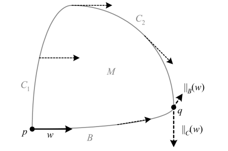
Figure 2.1: A vector $w$ transported in what we intuitively consider to be a “parallel” way along two different paths ($B$ and $C=C_{1}+C_{2}$) on a surface results in two different vectors.

The parallel transporter is therefore a map

$$\parallel_{C}\colon T_{p}M\to T_{q}M,$$ (2.1)

where $C$ is a curve in $M$ from $p$ to $q$ and $T_{p}M$ is the tangent space at $p$ (see Section B.2). To match our intuition we also require that this map be linear (i.e. parallel transport is assumed to preserve the vector space structure of the tangent space); that it be the identity for vanishing $C$; that if $C=C_{1}+C_{2}$ then $\parallel_{C}=\parallel_{C_{2}}\parallel_{C_{1}}$; and that the dependence on $C$ be smooth (this is most easily defined in the context of fiber bundles, which we will not cover here). If we then choose a frame on $U\subset M$, we have bases for each tangent space that provide isomorphisms $T_{p}U\cong\mathbb{R}^{n}$, $T_{q}U\cong\mathbb{R}^{n}$. Thus the parallel transporter can be viewed as a map

$$\parallel^{\lambda}{}_{\mu}\colon\left\{C\right\}\to GL\left(n,\mathbb{R}\right)$$ (2.2)

from the set of curves on $U$ to the Lie group $GL\left(n,\mathbb{R}\right)$ of general linear transformations on $\mathbb{R}^{n}$; however, it is important to note that the values of $\parallel^{\lambda}{}_{\mu}$ depend upon the choice of frame.

2.2 The covariant derivative

Having defined the parallel transporter, we can now consider the covariant derivative

$$\nabla_{v}w \equiv\underset{\varepsilon\rightarrow 0}{\textrm{lim}}\frac{1}{\varepsilon}\left(w\left|{}_{p+\varepsilon v}\right.-\parallel_{C}\left(w\left|{}_{p}\right.\right)\right)$$ (2.3)

$$=\underset{\varepsilon\rightarrow 0}{\textrm{lim}}\frac{1}{\varepsilon}\left(\parallel_{-C}\left(w\left|{}_{p+\varepsilon v}\right.\right)-w\left|{}_{p}\right.\right),$$

where $C$ is an infinitesimal curve starting at $p$ with tangent $v$. At a point $p$, $\nabla_{v}w$ compares the value of $w$ at $p+\varepsilon v$ to its value at $p$ after being parallel transported to $p+\varepsilon v$, or equivalently in the limit $\varepsilon\rightarrow 0$, the value of $w$ at $p$ to its value at $p+\varepsilon v$ after being parallel transported back to $p$. (see Section B.2 on how $p+\varepsilon v$ is well-defined in the limit $\varepsilon\rightarrow 0$).

Figure 2.2: The covariant derivative $\nabla_{v}w$ is the difference between a vector field $w$ and its parallel transport in the direction $v$.

☼ In this and future depictions of vector derivatives, the situation is simplified by focusing on the change in the vector field $w$ while showing the “transport” of $w$ as a parallel displacement. This has the advantage of highlighting the equivalency of defining the derivative at either 0 or $\varepsilon$ in the limit $\varepsilon\rightarrow 0$. Depicting $\parallel_{C}\left(w\left|{}_{p}\right.\right)$ as a non-parallel vector at $p+\varepsilon v$ would be more accurate, but would obscure this fact. We also will follow the picture here in using words to characterize derivatives: namely, “the difference” is short for “the difference per unit $\varepsilon$ to order $\varepsilon$ in the limit $\varepsilon\rightarrow 0$.”

Two properties of $\nabla_{v}w$ that are easy to verify are that is is linear in $v$, and that for a function $f$ on $M$ it obeys the rule

$$\nabla_{v}\left(fw\right) =v\left(f\right)w+f\nabla_{v}\left(w\right)$$ (2.4)

$$=\mathrm{d}f\left(v\right)w+f\nabla_{v}\left(w\right).$$

As we will see in Section 3.1, this is the Leibniz rule (see Appendix C.1) for the covariant derivative generalized to the tensor algebra. See Section B.6 for a review of the differential $\mathrm{d}$ and the relation $v(f)=\mathrm{d}f(v)$. Note that $\nabla_{v}w$ is a directional derivative, i.e. it depends only upon the value of $v$ at $p$; $v$ is in effect used only to choose a direction. In contrast, the Lie derivative $L_{v}w$ (see Section C.2) requires $v$ to be a vector field, since $w$ is in this case compared to its value after being “transported” by the local flow of $v$, and so depends on the derivative of $v$ at $p$.

$\triangle$ It is important to remember that there is no way to “transport” a vector on a manifold without introducing some extra structure.

Instead of parallel transport, one can consider the covariant derivative as the fundamental structure being added to the manifold. In this case it is useful to define the covariant derivative along a smooth parametrized curve $C(t)$ by using the tangent to the curve as the direction, i.e.

$$\frac{\mathrm{D}}{\mathrm{d}t}w\equiv\mathrm{D}_{t}w\equiv\nabla_{\dot{C}(t)}w,$$ (2.5)

where $\dot{C}(t)$ is the tangent to $C$ at $t$. $\mathrm{D}_{t}w$ is sometimes called the absolute derivative (AKA intrinsic derivative) and its definition only requires that $w$ be defined along the curve $C(t)$. We can then define the parallel transport of $w\left|{}_{p}\right.$ along $C(t)$ as the vector field $w$ that satisfies $\mathrm{D}_{t}w=0$.

$\triangle$ The notation for the absolute derivative is potentially confusing since the implicitly referenced curve $C(t)$ does not appear in the expression $\mathrm{D}_{t}w$.

2.3 The connection

If we view $\nabla$ as a map from two vector fields $v$ and $w$ to a third vector field $\nabla_{v}w$, it is called an affine connection. Note that since no use has been made of coordinates or frames in the definition of $\nabla$, it is a frame-independent quantity (see Appendix B for a review of coordinates and frames).

Since $\nabla_{v}$ is linear in $v$, and depends only on its local value, we can regard $\nabla$ as a 1-form on $M$. If we choose a frame $e_{\mu}$ on $M$ with corresponding dual frame $\beta^{\mu}$, we can define the connection 1-form

$$\Gamma^{\lambda}{}_{\mu}\left(v\right)\equiv\beta^{\lambda}\left(\nabla_{v}e_{\mu}\right).$$ (2.6)

$\Gamma^{\lambda}{}_{\mu}\left(v\right)$ is the $\lambda^{\textrm{th}}$ component of the difference between the frame $e_{\mu}$ and its parallel transport in the direction $v$.

From its definition, it is clear that $\Gamma^{\lambda}{}_{\mu}$ is a frame-dependent object, and additionally it is not local since it is formed from the derivative of the frame; therefore it cannot be viewed as the components of a tensor (see Appendix A for a review of tensors and forms).

At a point $p$, the value of $\Gamma^{\lambda}{}_{\mu}\left(v\right)$ is an infinitesimal linear transformation on $T_{p}M$, i.e. $\Gamma^{\lambda}{}_{\mu}$ is a frame-dependent 1-form whose values sit in the Lie algebra $gl\left(n,\mathbb{R}\right)$. Using the notation for algebra- and vector-valued forms defined in Section A.9, we can then write

$$\check{\Gamma}\left(v\right)\vec{w}\equiv\Gamma^{\lambda}{}_{\mu}\left(v\right)w^{\mu}e_{\lambda}=\left(\nabla_{v}e_{\mu}\right)w^{\mu},$$ (2.7)

where we view $\vec{w}$ as a $\mathbb{R}^{n}$-valued 0-form. The vector $\check{\Gamma}\left(v\right)\vec{w}$ measures the difference between the frame and its parallel transport in the direction $v$, weighted by the components of $w$.

$\triangle$ It is important to remember that $\check{\Gamma}\left(v\right)\vec{w}$ is related to the difference between the frame and its parallel transport, while $\nabla_{v}w$ measures the difference between $w$ and its parallel transport; thus unlike $\nabla_{v}w$, $\check{\Gamma}\left(v\right)\vec{w}$ depends only upon the local value of $w$, but takes values that are frame-dependent.

$\triangle$ Since we have used the frame to view $\check{\Gamma}$ as a $gl\left(n,\mathbb{R}\right)$-valued 1-form, i.e. a matrix-valued 1-form, $\vec{w}$ must be viewed as a frame-dependent column vector of components. We could instead view $\check{\Gamma}$ as a $gl\left(\mathbb{R}^{n}\right)$-valued 1-form and $\vec{w}$ as a frame-independent intrinsic vector. In this case the action of $\check{\Gamma}$ on $\vec{w}$ would be frame-independent, but the value of $\check{\Gamma}$ itself would remain frame-dependent. We choose to use matrix-valued forms due to the need below to take the exterior derivative of component functions, but the abstract viewpoint is important to keep in mind when generalizing to fiber bundles.

2.4 The covariant derivative in terms of the connection

$\nabla_{v}w$ can be written in terms of $\check{\Gamma}$ by using the Leibniz rule from Section 2.2 with $w^{\mu}$ as frame-dependent functions:

$$\nabla_{v}w =\nabla_{v}\left(w^{\mu}e_{\mu}\right)$$ (2.8)

$$=v\left(w^{\mu}\right)e_{\mu}+w^{\mu}\nabla_{v}\left(e_{\mu}\right)$$

$$=\mathrm{d}w^{\mu}\left(v\right)e_{\mu}+\check{\Gamma}\left(v\right)\vec{w}$$

$$\equiv\mathrm{d}\vec{w}\left(v\right)+\check{\Gamma}\left(v\right)\vec{w}$$

Here we again view $\vec{w}$ as a $\mathbb{R}^{n}$-valued 0-form, so that $\mathrm{d}\vec{w}\left(v\right)\equiv\mathrm{d}w^{\mu}\left(v\right)e_{\mu}$. Thus $\mathrm{d}\vec{w}\left(v\right)$ is the change in the components of $w$ in the direction $v$, making it frame-dependent even though $w$ is not. Note that although $\nabla_{v}w$ is a frame-independent quantity, both terms on the right hand side are frame-dependent. This is depicted in the following figure.

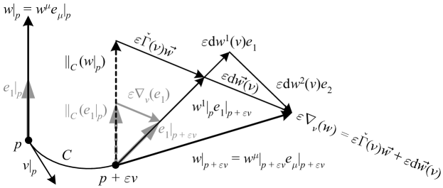
Figure 2.3: Relationships between the frame, parallel transport, covariant derivative, and connection for a vector $w$ parallel to $e_{1}$ at a point $p$.

$\sun$ The relation $\nabla_{v}w=\check{\Gamma}\left(v\right)\vec{w}+\mathrm{d}\vec{w}\left(v\right)$ can be viewed as roughly saying that the change in $w$ under parallel transport is equal to the change in the frame relative to its parallel transport plus the change in the components of $w$ in that frame.

If the 1-form $\Gamma^{\lambda}{}_{\mu}\left(v\right)$ itself is written using component notation, we arrive at the connection coefficients

$$\Gamma^{\lambda}{}_{\mu\sigma}\equiv\Gamma^{\lambda}{}_{\mu}\left(e_{\sigma}\right)=\beta^{\lambda}\left(\nabla_{e_{\sigma}}e_{\mu}\right).$$ (2.9)

$\Gamma^{\lambda}{}_{\mu\sigma}$ thus measures the $\lambda^{\mathrm{th}}$ component of the difference between $e_{\mu}$ and its parallel transport in the direction $e_{\sigma}$.

$\triangle$ This notation is potentially confusing, as it makes $\Gamma^{\lambda}{}_{\mu\sigma}$ look like the components of a tensor, which it is not: it is a derivative of the component of the frame indexed by $\mu$, and therefore is not only locally frame-dependent but also depends upon values of the frame at other points, so that it is not a multilinear mapping on its local arguments. Similarly, $\mathrm{d}\vec{w}$ looks like a frame-independent exterior derivative, but it is not: it is the exterior derivative of the frame-dependent components of $w$.

$\triangle$ The ordering of the lower indices of $\Gamma^{\lambda}{}_{\mu\sigma}$ is not consistent across the literature (e.g. [9] vs [7]). This is sometimes not remarked upon, possibly due to the fact that in typical circumstances in general relativity (a coordinate frame and zero torsion, to be defined in Section 3.4), the connection coefficients are symmetric in their lower indices.

It is common to extend abstract index notation (see Section A.4) to be able to express the covariant derivative in terms of the connection coefficients as follows:

$$\nabla_{e_{\mu}}w =\mathrm{d}w^{\lambda}\left(e_{\mu}\right)e_{\lambda}+\Gamma^{\lambda}{}_{\sigma}\left(e_{\mu}\right)w^{\sigma}e_{\lambda}$$ (2.10)

$$\Rightarrow\nabla_{a}w^{b}\equiv\left(\nabla_{e_{a}}w\right)^{b} =e_{a}\left(w^{b}\right)+\Gamma^{b}{}_{ca}w^{c}$$

$$\Rightarrow\nabla_{a}w^{b} =\partial_{a}w^{b}+\Gamma^{b}{}_{ca}w^{c}$$

Here we have also defined $\partial_{a}f\equiv\partial_{e_{a}}f=\mathrm{d}f(e_{a})=e_{a}(f)$, which is then extended to $\partial_{v}f\equiv v^{a}\partial_{a}f$. This notation is also sometimes supplemented to use a comma to indicate partial differentiation and a semicolon to indicate covariant differentiation, so that the above becomes

$$w^{b}{}_{;a}=w^{b}{}_{,a}+\Gamma^{b}{}_{ca}w^{c}.$$ (2.11)

The extension of index notation to derivatives has several potentially confusing aspects:

• $\nabla_{a}$ and $\partial_{a}$ written alone are not 1-forms

• Greek indices indicate only that a specific basis (frame) has been chosen ([9] pp. 23-26), but do not distinguish between a general frame, where $\partial_{\mu}f\equiv\mathrm{d}f(e_{\mu})$, and a coordinate frame, where $\partial_{\mu}f\equiv\partial f/\partial x^{\mu}$

• $\nabla_{a}w^{b}\equiv(\nabla_{e_{a}}w)^{b}$, so since $\nabla_{v}w$ is linear in $v$, $\nabla_{a}w^{b}$ is in fact a tensor of type $\left(1,1\right)$; a more accurate notation might be $(\nabla w)^{b}{}_{a}$

• $w^{b}$ in the expression $\partial_{a}w^{b}\equiv\mathrm{d}w^{b}(e_{a})$ is not a vector, it is a set of frame-dependent component functions labeled by $b$ whose change in the direction $e_{a}$ is being measured

• The above means that, consistent with the definition of the connection coefficients, we have $\nabla_{a}e_{b}=0+e_{c}\Gamma^{c}{}_{ba}$, since the components of the frame itself by definition do not change

• When using a coordinate frame based on curvilinear coordinates in Euclidean space, parallel transport is implicit in taking partial derivatives of vectors, resulting in the above being expressed as $\partial_{\mu}e_{\lambda}=e_{\sigma}\Gamma^{\sigma}{}_{\lambda\mu}$

• As previously noted, neither $\Gamma^{b}{}_{ca}$ nor $\Gamma^{b}{}_{ca}w^{c}$ are tensors

We will nevertheless use this notation for many expressions going forward, as it is frequently used in general relativity.

$\triangle$ It is important to remember that expressions involving $\nabla_{a}$, $\partial_{a}$, and $\Gamma^{c}{}_{ba}$ must be handled carefully, as none of these are consistent with the original concept of indices denoting tensor components.

$\triangle$ Some texts will distinguish between the labels of basis vectors and abstract index notation by using expressions such as $(e_{i})^{a}$. We will not follow this practice, as it makes difficult the convenient method of matching indexes in expressions such as $\partial_{a}w^{b}\equiv\mathrm{d}w^{b}(e_{a})$.

$\triangle$ If we choose coordinates $x^{\mu}$ and use a coordinate frame so that $\partial_{\mu}\equiv\partial/\partial x^{\mu}$, we have the usual relation $\partial_{\mu}\partial_{\nu}f=\partial_{\nu}\partial_{\mu}f$. However, this is not necessarily implied by the Greek indices alone, which only indicate that a particular frame has been chosen. For index notation in general, mixed partials do not commute, since $\partial_{a}\partial_{b}f-\partial_{b}\partial_{a}f=e_{a}(e_{b}(f))-e_{b}(e_{a}(f))=[e_{a},e_{b}](f)=[e_{a},e_{b}]^{c}\partial_{c}f$, which only vanishes in a holonomic frame.

2.5 The parallel transporter in terms of the connection

We can also consider the parallel transport of a vector $w$ along an infinitesimal curve $C$ with tangent $v$. Referring to Fig. 2.3, we see that to order $\varepsilon$ the components $w^{\mu}$ transform according to

$$\parallel^{\lambda}{}_{\mu}\left(C\right)w^{\mu}=w^{\lambda}-\varepsilon\Gamma^{\lambda}{}_{\mu}\left(v\right)w^{\mu},$$ (2.12)

where $v$ is tangent to the curve $C$, and these components are with respect to the frame at the new point after infinitesimal parallel transport. Using this relation, we can build up a frame-dependent expression for the parallel transporter for finite $C$ by multiplying terms $\left(1-\varepsilon\Gamma\left|{}_{p}\right.\right)$ where $\Gamma\left|{}_{p}\right.$ is used to denote the matrix $\Gamma^{\lambda}{}_{\mu}\left(v\left|{}_{p}\right.\right)$ evaluated on the tangent $v\left|{}_{p}\right.$ at successive points $p$ along $C$. The limit of this process is the path-ordered exponential

$$\parallel^{\lambda}{}_{\mu}\left(C\right) =\underset{\varepsilon\rightarrow 0}{\textrm{lim}}\left(1-\varepsilon\Gamma\left|{}_{q-\varepsilon}\right.\right)\left(1-\varepsilon\Gamma\left|{}_{q-2\varepsilon}\right.\right)\dotsm\left(1-\varepsilon\Gamma\left|{}_{p+\varepsilon}\right.\right)\left(1-\varepsilon\Gamma\left|{}_{p}\right.\right)$$ (2.13)

$$\equiv P\textrm{exp}\left(-\underset{C}{\int}\Gamma^{\lambda}{}_{\mu}\right),$$

whose definition is based on the expression for the exponential

$$e^{x}=\underset{n\rightarrow\infty}{\textrm{lim}}\left(1+\frac{x}{n}\right)^{n}=\underset{\varepsilon\rightarrow 0}{\textrm{lim}}\left(1+\varepsilon x\right)^{1/\varepsilon}.$$ (2.14)

Note that the above expression for $\parallel^{\lambda}{}_{\mu}\left(C\right)$ exponentiates frame-dependent values in $gl\left(n,\mathbb{R}\right)$ to yield a frame-dependent value in $GL\left(n,\mathbb{R}\right)$.

2.6 Geodesics and normal coordinates

Following the example of the Lie derivative (see Section C.2), we can consider parallel transport of a vector $v$ in the direction $v$ as generating a local flow. More precisely, for any vector $v$ at a point $p\in M$, there is a curve $\phi_{v}(t)$, unique for some $-\varepsilon<t<\varepsilon$, such that $\phi_{v}(0)=p$ and $\dot{\phi}_{v}\left(t\right)=\parallel_{\phi}(v)$, the last expression indicating that the tangent to $\phi_{v}$ at $t$ is equal to the parallel transport of $v$ along $\phi_{v}$ from $\phi_{v}(0)$ to $\phi_{v}(t)$. This curve is called a geodesic, and its tangent vectors are all parallel transports of each other. This means that for all tangent vectors $v$ to the curve, $\nabla_{v}v=0$, so that geodesics are “the closest thing to straight lines” on a manifold with parallel transport.

Expressing a geodesic as a parametrized curve $C^{\mu}(t)$ with tangent $v^{\mu}\left(t\right)\equiv\dot{C}^{\mu}\left(t\right)$ in given coordinates, we can write

$$\nabla_{v}v =v^{\lambda}\left(\partial_{\lambda}v^{\mu}+\Gamma^{\mu}{}_{\sigma\lambda}v^{\sigma}\right)$$ (2.15)

$$=\partial_{v}\left(v^{\mu}\right)+\Gamma^{\mu}{}_{\sigma\lambda}v^{\sigma}v^{\lambda}$$

$$=\frac{\mathrm{d}}{\mathrm{d}t}\left(\frac{\mathrm{d}C^{\mu}}{\mathrm{d}t}\right)+\Gamma^{\mu}{}_{\sigma\lambda}\frac{\mathrm{d}C^{\sigma}}{\mathrm{d}t}\frac{\mathrm{d}C^{\lambda}}{\mathrm{d}t}$$

$$=\frac{\mathrm{d}^{2}C^{\mu}}{\mathrm{d}t^{2}}+\Gamma^{\mu}{}_{\sigma\lambda}\frac{\mathrm{d}C^{\sigma}}{\mathrm{d}t}\frac{\mathrm{d}C^{\lambda}}{\mathrm{d}t}=0,$$

where the last line is called the geodesic equation, and in the third line we use the fact that the change of the 0-form $v^{\mu}$ in the $v$ direction is equal to the derivative of the function $v^{\mu}\left(t\right)$ with respect to $t$.

Now we can define the exponential map at $p$ to be $\mathrm{exp}(v)\equiv\phi_{v}(1)$, which will be well-defined for values of $v$ around the origin that map to some $U\subset M$ containing $p$. Finally, choosing a basis for $T_{p}U$ provides an isomorphism $T_{p}U\cong\mathbb{R}^{n}$, allowing us to define geodesic normal coordinates (AKA normal coordinates) $\mathrm{exp}^{-1}\colon U\to\mathbb{R}^{n}$. It can be shown (see [6] Vol. 1 pp148-149) that in a coordinate frame at the origin $p$ of geodesic normal coordinates, we have $\Gamma^{\lambda}{}_{\mu\sigma}=-\Gamma^{\lambda}{}_{\sigma\mu}$; this implies that for zero torsion (to be defined in Section 3.4), the connection coefficients vanish at $p$.

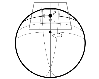
Figure 2.4: Geodesic normal coordinates at $p$ map points on a manifold to vectors at $p$ tangent to the geodesic passing through both points. In the figure $\mathrm{exp}(2v)=\phi_{v}(2)$, so the coordinate of the point $\phi_{v}(2)\in M$ is $2v\in T_{p}M$.

2.7 Summary

In general, a “manifold with connection” is one with an additional structure that “connects” the different tangent spaces of the manifold to one another in a linear fashion. Specifying any one of the above connection quantities, the covariant derivative, or the parallel transporter equivalently determines this structure. The following tables summarize the situation.

Construct	Argument(s)	Value	Dependencies
$\parallel_{C}$	$v\in T_{p}M$	$\parallel_{C}\left(v\right)\in T_{q}M$	Path $C$ from $p$ to $q$
$\parallel^{\lambda}{}_{\mu}$	Path $C$	$\parallel^{\lambda}{}_{\mu}\left(C\right)\in GL$	Frame on $M$
$\nabla_{v}$	$w\in TM$	$\nabla_{v}w\in T_{p}M$	$v\in T_{p}M$
$\nabla$	$v\in T_{p}M$, $w\in TM$	$\nabla_{v}w\in T_{p}M$	None
$\Gamma^{\lambda}{}_{\mu}$	$v\in T_{p}M$	$\Gamma^{\lambda}{}_{\mu}\left(v\right)\in gl$	Frame on $M$
$\check{\Gamma}\left(v\right)$	$\vec{w}\in T_{p}M$	$\check{\Gamma}\left(v\right)\vec{w}\in T_{p}M$	Frame on $M$, $v\in T_{p}M$
$\Gamma^{\lambda}{}_{\mu\sigma}$	None	Connection coefficient	Frame on $M$

Table 2.1: Constructions related to the connection. Each construct above is considered at a point $p$; to determine a manifold with connection it must be defined for every point in $M$.

Below we review the intuitive meanings of the various vector derivatives.

Vector derivative	Meaning
$L_{v}w\equiv\underset{\varepsilon\rightarrow 0}{\textrm{lim}}\left(w\left|{}_{p+\varepsilon v}\right.-\mathrm{d}\Phi_{\varepsilon}\left(w\left|{}_{p}\right.\right)\right)/\varepsilon$	The difference between $w$ and its transport by the local flow of $v$.
$\nabla_{v}w\equiv\underset{\varepsilon\rightarrow 0}{\textrm{lim}}\left(w\left|{}_{p+\varepsilon v}\right.-\parallel_{C}\left(w\left|{}_{p}\right.\right)\right)/\varepsilon$	The difference between $w$ and its parallel transport in the direction $v$.
$\frac{\mathrm{D}}{\mathrm{d}t}w\equiv\mathrm{D}_{t}w\equiv\nabla_{\dot{C}(t)}w$	The difference between $w$ and its parallel transport in the direction tangent to $C(t)$.
$\Gamma^{\lambda}{}_{\mu}\left(v\right)\equiv\beta^{\lambda}\left(\nabla_{v}e_{\mu}\right)$	The $\lambda^{\textrm{th}}$ component of the difference between $e_{\mu}$ and its parallel transport in the direction $v$.
$\check{\Gamma}\left(v\right)\equiv\nabla_{v}\left(T_{p}M\right)$	The infinitesimal linear transformation on the tangent space that takes the parallel transported frame to the frame in the direction $v$.
$\check{\Gamma}\left(v\right)\vec{w}\equiv\Gamma^{\lambda}{}_{\mu}\left(v\right)w^{\mu}e_{\lambda}=\left(\nabla_{v}e_{\mu}\right)w^{\mu}$	The difference between the frame and its parallel transport in the direction $v$, weighted by the components of $w$.
$\Gamma^{\lambda}{}_{\mu\sigma}\equiv\Gamma^{\lambda}{}_{\mu}\left(e_{\sigma}\right)=\beta^{\lambda}\left(\nabla_{\sigma}e_{\mu}\right)$	The $\lambda^{\textrm{th}}$ component of the difference between $e_{\mu}$ and its parallel transport in the direction $e_{\sigma}$.
$\mathrm{d}\vec{w}\left(v\right)\equiv\mathrm{d}w^{\mu}\left(v\right)e_{\mu}$	The change in the frame-dependent components of $w$ in the direction $v$.
$\partial_{a}w^{b}\equiv\mathrm{d}w^{b}(e_{a})$	The change in the $b^{\mathrm{th}}$ frame-dependent component of $w$ in the direction $e_{a}$.
$\nabla_{a}w^{b}\equiv(\nabla_{e_{a}}w)^{b}$	The $b^{\mathrm{th}}$ component of the difference between $w$ and its parallel transport in the direction $e_{a}$.

Table 2.2: Definitions and meanings of vector derivatives.

Other quantities in terms of the connection:

• $\nabla_{v}w=\mathrm{d}\vec{w}\left(v\right)+\check{\Gamma}\left(v\right)\vec{w}$

• $\nabla_{a}w^{b}=\partial_{a}w^{b}+\Gamma^{b}{}_{ca}w^{c}$

• $\parallel^{\lambda}{}_{\mu}\left(C\right)w^{\mu}=w^{\mu}-\varepsilon\Gamma^{\lambda}{}_{\mu}\left(v\right)w^{\mu}$   (for infinitesimal $C$ with tangent $v$)

• $\parallel^{\lambda}{}_{\mu}\left(C\right)w^{\mu}=P\textrm{exp}\left(-\int_{C}\Gamma^{\lambda}{}_{\mu}\right)w^{\mu}$

3 Manifolds with connection

All of the above constructs used to define a manifold with connection manipulate vectors, which means they can be naturally extended to operate on arbitrary tensor fields on $M$. This is the usual approach taken in general relativity; however, one can alternatively focus on $k$-forms on $M$, an approach that generalizes more directly to gauge theories in physics. This viewpoint is sometimes called the Cartan formalism. We will cover both approaches.

$\triangle$ Note that a manifold with connection includes no concept of length or distance (a metric). It is important to remember that unless noted, nothing in this section depends upon this extra structure.

3.1 The covariant derivative on the tensor algebra

If we define the covariant derivative of a function to coincide with the normal derivative, i.e. $\nabla_{a}f\equiv\partial_{a}f$, then we can use the Leibniz rule to define the covariant derivative of a 1-form. This is sometimes described as making the covariant derivative “commute with contractions,” where for a 1-form $\varphi$ and a vector $v$ we require

$$\nabla_{a}\left(\varphi_{b}v^{b}\right) \equiv\left(\nabla_{a}\varphi_{b}\right)v^{b}+\varphi_{b}\left(\nabla_{a}v^{b}\right)$$ (3.1)

$$=\left(\nabla_{a}\varphi_{b}\right)v^{b}+\varphi_{b}\left(\partial_{a}v^{b}+\Gamma^{b}{}_{ca}v^{c}\right).$$

At the same time, choosing a frame and treating $\varphi_{b}$ and $v^{b}$ as frame-dependent functions on $M$, we have

$$\nabla_{a}\left(\varphi_{b}v^{b}\right) \equiv\partial_{a}\left(\varphi_{b}v^{b}\right)$$ (3.2)

$$=\left(\partial_{a}\varphi_{b}\right)v^{b}+\varphi_{b}\left(\partial_{a}v^{b}\right),$$

so that equating the two we arrive at

$$\nabla_{a}\varphi_{b}\equiv\partial_{a}\varphi_{b}-\Gamma^{c}{}_{ba}\varphi_{c}.$$ (3.3)

As with vectors, the partial derivative $\partial_{a}\varphi_{b}$ acts upon the frame-dependent components of the 1-form.

We can then extend the covariant derivative to be a derivation on the tensor algebra (see Section C.1) by following the above logic for each covariant and contravariant component:

$$\nabla_{a}T^{b_{1}\ldots b_{m}}{}_{c_{1}\ldots c_{n}} \equiv\partial_{a}T^{b_{1}\ldots b_{m}}{}_{c_{1}\ldots c_{n}}$$ (3.4)

$$\phantom{{}=}+\underset{j=1}{\overset{m}{\sum}}\Gamma^{b_{j}}{}_{da}T^{b_{1}\ldots b_{j-1}db_{j+1}\ldots b_{m}}{}_{c_{1}\ldots c_{n}}$$

$$\phantom{{}=}-\underset{j=1}{\overset{n}{\sum}}\Gamma^{d}{}_{c_{j}a}T^{b_{1}\ldots b_{m}}{}_{c_{1}\ldots c_{j-1}dc_{j+1}\ldots c_{n}}$$

Note that since the covariant derivative of a 0-form is $\nabla_{a}f=\partial_{a}f=\partial_{e_{a}}f=e_{a}(f)$, we then have $\nabla_{v}f=v^{a}\nabla_{a}f=v^{a}e_{a}(f)=v(f)$.

The concept of parallel transport along a curve $C$ can be extended to the tensor algebra as well, by parallel transporting all vector arguments backwards to the starting point of $C$, applying the tensor, then parallel transporting the resulting vectors forward to the endpoint of $C$. So for example the parallel transport of a tensor $T^{a}{}_{b}$ is defined as

$$\parallel_{C}\left(T^{a}{}_{b}\right) \equiv?\parallel^{a}{}_{c}?\left(C\right)?T^{c}{}_{d}??\parallel^{d}{}_{b}?\left(-C\right)$$ (3.5)

$$=\left(1-\varepsilon?\Gamma^{a}{}_{c}?\left(v\right)\right)?T^{c}{}_{d}?\left(1+\varepsilon?\Gamma^{d}{}_{b}?\left(v\right)\right),$$

where for infinitesimal $C$ with tangent $v$ we have $\parallel_{C}^{-1}=\parallel_{-C}=1+\varepsilon\check{\Gamma}\left(v\right)$ since $\parallel_{C}=1-\varepsilon\check{\Gamma}\left(v\right)$.

Figure 3.1: The parallel transport of a tensor can be defined by parallel transporting all vector arguments backwards to the starting point, applying the tensor, then parallel transporting the resulting vectors forward to the endpoint.

With this definition, the covariant derivative $\nabla_{a}T$ can be viewed as “the difference between $T$ and its parallel transport in the direction $e_{a}$.”

$\triangle$ It can sometimes be confusing when using the extended covariant derivative as to what type of tensor it is being applied to. For example, $w^{b}$ in the expression $\partial_{a}w^{b}$ is not a vector, it is a set of frame-dependent functions labeled by $b$; yet this expression can in theory also be written $\nabla_{a}w^{b}$, in which case there is no indication that the covariant derivative is acting on these functions instead of the vector $w^{b}$.

$\triangle$ When the covariant derivative is used as a derivation on the tensor algebra, care must be taken with relations, since their forms can change considerably based upon what arguments are applied and whether index notation is used. In particular, $(\nabla_{a}\nabla_{b}-\nabla_{b}\nabla_{a})f=\nabla_{a}(\partial_{b}f)-\nabla_{b}(\partial_{a}f)$ is not a “mixed partials” expression, since $(\partial_{a}f)$ is a 1-form. And as we will see, $(\nabla_{a}\nabla_{b}-\nabla_{b}\nabla_{a})f$ is a different construction than $(\nabla_{a}\nabla_{b}-\nabla_{b}\nabla_{a})w^{c}$, which is different from $(\nabla_{u}\nabla_{v}-\nabla_{v}\nabla_{u})w$. It is important to realize that an expression such as $\nabla_{a}\nabla_{b}-\nabla_{b}\nabla_{a}$ without context has no unambiguous meaning.

$\triangle$ It is important to remember that since expressions like $\partial_{a}w^{b}$ and $\Gamma^{c}{}_{ba}$ are not tensors, applying $\nabla_{d}$ to them is not well-defined (unless we consider them as arrays of functions and are applying $\nabla_{d}=\partial_{d}$).

3.2 The exterior covariant derivative of vector-valued forms

A vector field $w$ on $M$ can be viewed as a vector-valued 0-form. As noted previously, the covariant derivative $\nabla_{v}w$ is linear in $v$ and depends only on its local value, and so can be viewed as a vector-valued 1-form $\mathrm{D}\vec{w}(v)\equiv\nabla_{v}w$. $\mathrm{D}\vec{w}$ is called the exterior covariant derivative of the vector-valued 0-form $\vec{w}$. This definition is then extended to vector-valued $k$-forms $\vec{\varphi}$ by following the example of the exterior derivative $\mathrm{d}$ (see Section C.5):

$$\mathrm{D}\vec{\varphi}\left(v_{0},\dotsc,v_{k}\right)$$ (3.6)

$$\equiv\underset{j=0}{\overset{k}{\sum}}\left(-1\right)^{j}\nabla_{v_{j}}\left(\vec{\varphi}\left(v_{0},\dotsc,v_{j-1},v_{j+1},\dotsc,v_{k}\right)\right)$$

$$\phantom{{}=}+\underset{i<j}{\sum}\left(-1\right)^{i+j}\vec{\varphi}\left(\left[v_{i},v_{j}\right],v_{0},\dotsc,v_{i-1},v_{i+1},\dotsc,v_{j-1},v_{j+1},\dotsc,v_{k}\right)$$

For example, if $\vec{\varphi}$ is a vector-valued 1-form,

$$\mathrm{D}\vec{\varphi}\left(v,w\right)\equiv\nabla_{v}\vec{\varphi}\left(w\right)-\nabla_{w}\vec{\varphi}\left(v\right)-\vec{\varphi}\left(\left[v,w\right]\right).$$ (3.7)

So while the first term of $\mathrm{d}\varphi$ takes the difference between the scalar values of $\varphi(w)$ along $v$, the first term of $\mathrm{D}\vec{\varphi}$ takes the difference between the vector values of $\vec{\varphi}(w)$ along $v$ after parallel transporting them to the same point (which is required to compare them). At a point $p$, $\mathrm{D}\vec{\varphi}\left(v,w\right)$ can thus be viewed as the “sum of $\vec{\varphi}$ on the boundary of the surface defined by its arguments after being parallel transported back to $p$,” and if we use $\|_{\varepsilon v}$ to denote parallel transport along an infinitesimal curve with tangent $v$, we can write

$$\varepsilon^{2}\mathrm{D}\vec{\varphi}\left(v,w\right) =\|_{-\varepsilon v}\vec{\varphi}\left(\varepsilon w\left|{}_{p+\varepsilon v}\right.\right)-\vec{\varphi}\left(\varepsilon w\left|{}_{p}\right.\right)$$ (3.8)

$$-\|_{-\varepsilon w}\vec{\varphi}\left(\varepsilon v\left|{}_{p+\varepsilon w}\right.\right)+\vec{\varphi}\left(\varepsilon v\left|{}_{p}\right.\right)$$

$$-\vec{\varphi}\left(\varepsilon^{2}\left[v,w\right]\right).$$

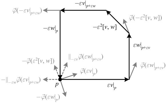
Figure 3.2: The exterior covariant derivative $\mathrm{D}\vec{\varphi}\left(v,w\right)$ sums the vectors $\vec{\varphi}$ along the boundary of the surface defined by $v$ and $w$ by parallel transporting them to the same point. Note that the “completion of the parallelogram” $[v,w]$ is already of order $\varepsilon^{2}$, so its parallel transport has no effect to this order.

From its definition, it is clear that $\mathrm{D}\vec{\varphi}$ is a frame-independent quantity. In terms of the connection, we must consider $\vec{w}$ as a frame-dependent $\mathbb{R}^{n}$-valued 0-form, so that

$$\mathrm{D}\vec{w}\left(v\right)=\nabla_{v}w=\mathrm{d}\vec{w}\left(v\right)+\check{\Gamma}\left(v\right)\vec{w}.$$ (3.9)

For a $\mathbb{R}^{n}$-valued $k$-form $\vec{\varphi}$ we find that

$$\mathrm{D}\vec{\varphi}=\mathrm{d}\vec{\varphi}+\check{\Gamma}\wedge\vec{\varphi},$$ (3.10)

where the exterior derivative is defined to apply to the frame-dependent components, i.e. $\mathrm{d}\vec{\varphi}(v_{0}\ldots v_{k})\equiv\mathrm{d}\varphi^{\mu}(v_{0}\ldots v_{k})e_{\mu}$. Recall that $\check{\Gamma}$ is a $gl(n,\mathbb{R})$-valued 1-form, so that for example if $\vec{\varphi}$ is a $\mathbb{R}^{n}$-valued 1-form then

$$(\check{\Gamma}\wedge\vec{\varphi})\left(v,w\right) \equiv\check{\Gamma}\left(v\right)\vec{\varphi}\left(w\right)-\check{\Gamma}\left(w\right)\vec{\varphi}\left(v\right)$$ (3.11)

$$=?\Gamma^{\lambda}{}_{\mu}?\left(v\right)\varphi^{\mu}\left(w\right)-?\Gamma^{\lambda}{}_{\mu}?\left(w\right)\varphi^{\mu}\left(v\right).$$

$\triangle$ As with the covariant derivative, it is important to remember that $\mathrm{D}\vec{\varphi}$ is frame-independent while $\mathrm{d}\vec{\varphi}$ and $\check{\Gamma}$ are not.

The set of vector-valued forms can be viewed as an infinite-dimensional algebra by defining multiplication via the vector field commutator; it turns out that $\mathrm{D}$ does not satisfy the Leibniz rule in this algebra and so is not a derivation (see Appendix C.1). However, following the above reasoning one can extend the definition of $\mathrm{D}$ to the algebra of tensor-valued forms, or the subset of anti-symmetric tensor-valued forms; $\mathrm{D}$ then is a derivation with respect to the tensor product in the former case and a graded derivation with respect to the exterior product in the latter case. We will not pursue either of these two generalizations.

3.3 The exterior covariant derivative of algebra-valued forms

Recalling from Section 3.1 the definition of parallel transport of a tensor, we can view a $gl(n,\mathbb{R})$-valued 0-form $\check{\Theta}$ as a tensor of type $\left(1,1\right)$, so that the infinitesimal parallel transport of $\check{\Theta}$ along $C$ with tangent $v$ is

$$\parallel_{C}(\check{\Theta})=\left(1-\varepsilon\check{\Gamma}\left(v\right)\right)\check{\Theta}\left(1+\varepsilon\check{\Gamma}\left(v\right)\right).$$ (3.12)

We can now follow the reasoning used to define the covariant derivative of a vector in terms of the connection

$$\nabla_{v}w \equiv\underset{\varepsilon\rightarrow 0}{\textrm{lim}}\frac{1}{\varepsilon}\left(w\left|{}_{p+\varepsilon v}\right.-\parallel_{C}w\left|{}_{p}\right.\right)$$ (3.13)

$$=\underset{\varepsilon\rightarrow 0}{\textrm{lim}}\frac{1}{\varepsilon}\left(\vec{w}\left|{}_{p+\varepsilon v}\right.-\left(1-\varepsilon\check{\Gamma}\left(v\right)\right)\vec{w}\left|{}_{p}\right.\right)$$

$$=\underset{\varepsilon\rightarrow 0}{\textrm{lim}}\frac{1}{\varepsilon}\left(w^{\mu}\left|{}_{p+\varepsilon v}\right.-w^{\mu}\left|{}_{p}\right.+\varepsilon?\Gamma^{\mu}{}_{\lambda}?\left(v\right)w^{\lambda}\left|{}_{p}\right.\right)e_{\mu}\left|{}_{p+\varepsilon v}\right.$$

$$=\mathrm{d}\vec{w}\left(v\right)+\check{\Gamma}\left(v\right)\vec{w}$$

to give the covariant derivative of a $gl(n,\mathbb{R})$-valued 0-form

$$\nabla_{v}\check{\Theta} \equiv\underset{\varepsilon\rightarrow 0}{\textrm{lim}}\frac{1}{\varepsilon}\left(\check{\Theta}\left|{}_{p+\varepsilon v}\right.-\parallel_{C}\left(\check{\Theta}\left|{}_{p}\right.\right)\right)$$ (3.14)

$$=\underset{\varepsilon\rightarrow 0}{\textrm{lim}}\frac{1}{\varepsilon}\left(\check{\Theta}\left|{}_{p+\varepsilon v}\right.-\left(1-\varepsilon\check{\Gamma}\left(v\right)\right)\check{\Theta}\left|{}_{p}\right.\left(1+\varepsilon\check{\Gamma}\left(v\right)\right)\right)$$

$$=\mathrm{d}\check{\Theta}\left(v\right)+\check{\Gamma}\left(v\right)\check{\Theta}-\check{\Theta}\check{\Gamma}\left(v\right)$$

$$=\mathrm{d}\check{\Theta}\left(v\right)+\left[\check{\Gamma},\check{\Theta}\right]\left(v\right)$$

$$=\mathrm{d}\check{\Theta}\left(v\right)+\left(\check{\Gamma}[\wedge]\check{\Theta}\right)\left(v\right).$$

Here we have only kept terms to order $\varepsilon$, followed previous convention to define $\mathrm{d}\check{\Theta}\left(v\right)\equiv\mathrm{d}?\Theta^{\mu}{}_{\lambda}?\beta^{\lambda}e_{\mu}$, and defined the Lie commutator $[\check{\Gamma},\check{\Theta}]$ in terms of the multiplication of the $gl(n,\mathbb{R})$-valued forms $\check{\Gamma}$ and $\check{\Theta}$, which (see Section A.9 for notation) as a 1-form is equivalent to $\check{\Gamma}[\wedge]\check{\Theta}$. $\nabla_{v}\check{\Theta}$ is then “the difference between the linear transformation $\check{\Theta}$ and its parallel transport in the direction $v$.”

The above definition of the covariant derivative can then be extended to arbitrary $gl(n,\mathbb{R})$-valued $k$-forms by defining

$$\mathrm{D}\check{\Theta}\equiv\mathrm{d}\check{\Theta}+\check{\Gamma}[\wedge]\check{\Theta},$$ (3.15)

which can be shown to be equivalent to the construction used for $\mathbb{R}^{n}$-valued $k$-forms in Section 3.2. For example, for a $gl(n,\mathbb{R})$-valued 1-form $\check{\Theta}$, we have

$$\mathrm{D}\check{\Theta}\left(v,w\right)\equiv\nabla_{v}\check{\Theta}\left(w\right)-\nabla_{w}\check{\Theta}\left(v\right)-\check{\Theta}\left(\left[v,w\right]\right),$$ (3.16)

with the covariant derivatives acting on the value of $\check{\Theta}$ as a tensor of type $\left(1,1\right)$. So at a point $p$, $\mathrm{D}\check{\Theta}\left(v,w\right)$ can be viewed as the “sum of $\check{\Theta}$ on the boundary of the surface defined by its arguments after being parallel transported back to $p$.” With respect to the set of $gl(n,\mathbb{R})$-valued forms under the exterior product using the Lie commutator $[\wedge]$, $\mathrm{D}$ is a graded derivation and for a $gl(n,\mathbb{R})$-valued $k$-form $\check{\Theta}$ satisfies the Leibniz rule

$$\mathrm{D}(\check{\Theta}[\wedge]\check{\Psi})=\mathrm{D}\check{\Theta}[\wedge]\check{\Psi}+\left(-1\right)^{k}\check{\Theta}[\wedge]\mathrm{D}\check{\Psi}.$$ (3.17)

3.4 Torsion

Given a frame $e_{\mu}$, we can view the dual frame $\beta^{\mu}$ as a vector-valued 1-form that simply returns its vector argument:

$$\vec{\beta}\left(v\right)\equiv\beta^{\mu}\left(v\right)e_{\mu}=v.$$ (3.18)

Clearly this is a frame-independent object. The torsion is then defined to be the exterior covariant derivative

$$\vec{T}\equiv\mathrm{D}\vec{\beta}.$$ (3.19)

In terms of the connection, we must consider $\vec{\beta}$ as a frame-dependent $\mathbb{R}^{n}$-valued 1-form, which gives us the torsion as a $\mathbb{R}^{n}$-valued 2-form

$$\vec{T}=\mathrm{d}\vec{\beta}+\check{\Gamma}\wedge\vec{\beta}.$$ (3.20)

This definition of $\vec{T}$ is sometimes called Cartan’s first structure equation.

In terms of the covariant derivative, the torsion 2-form is

$$\vec{T}\left(v,w\right) \equiv\nabla_{v}\left(\vec{\beta}\left(w\right)\right)-\nabla_{w}\left(\vec{\beta}\left(v\right)\right)-\vec{\beta}\left(\left[v,w\right]\right)$$ (3.21)

$$=\nabla_{v}w-\nabla_{w}v-\left[v,w\right].$$

For a torsion-free connection in a holonomic frame, we then have $\nabla_{\sigma}e_{\mu}=\nabla_{\mu}e_{\sigma}$, which means that the connection coefficients are symmetric in their lower indices, i.e.

$$?\Gamma^{\lambda}{}_{\mu\sigma}?\equiv\beta^{\lambda}\left(\nabla_{\sigma}e_{\mu}\right)=\beta^{\lambda}\left(\nabla_{\mu}e_{\sigma}\right)=?\Gamma^{\lambda}{}_{\sigma\mu}?.$$ (3.22)

For this reason, a torsion-free connection is also called a symmetric connection.

From the definition in terms of the exterior covariant derivative, we can view the torsion as the “sum of the boundary vectors of the surface defined by its arguments after being parallel transported back to $p$,” i.e. the torsion measures the amount by which the boundary of a loop fails to close after being parallel transported. From the definition in terms of the covariant derivative, we arrive in the figure below at another interpretation where, like the Lie derivative $L_{v}w$ (see Section C.2), $\vec{T}(v,w)$ “completes the parallelogram” formed by its vector arguments, but this parallelogram is formed by parallel transport instead of local flow. Note however that the torsion vector has the opposite sign as the Lie derivative.

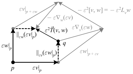
Figure 3.3: The torsion vector $\vec{T}\left(v,w\right)$, constructed above starting at the point $q$, “completes the parallelogram” formed by parallel transport. $\|_{\varepsilon v}$ denotes parallel transport along an infinitesimal curve with tangent $v$.

Zero torsion then means that moving infinitesimally along $v$ followed by the parallel transport of $w$ is the same as moving infinitesimally along $w$ followed by the parallel transport of $v$. Non-zero torsion signifies that “a loop made of parallel transported vectors is not closed.”

As this geometric interpretation suggests, and as is evident from the expression $\vec{T}\equiv\mathrm{D}\vec{\beta}$, one can verify algebraically that despite being defined in terms of derivatives $\vec{T}(v,w)$ in fact only depends on the local values of $v$ and $w$, and thus can be viewed as a tensor of type $\left(1,2\right)$:

$$?T^{c}{}_{ab}?v^{a}w^{b}\equiv v^{a}\nabla_{a}w^{c}-w^{a}\nabla_{a}v^{c}-[v,w]^{c}$$ (3.23)

Another relation can be obtained for the torsion tensor by applying its vector value to a function $f$ before moving into index notation:

$$\vec{T}\left(v,w\right)(f) \equiv\left(\nabla_{v}w\right)(f)-\left(\nabla_{w}v\right)(f)-\left[v,w\right](f)$$ (3.24)

$$\Rightarrow?T^{c}{}_{ab}?v^{a}w^{b}\nabla_{c}f =\left(v^{a}\nabla_{a}w^{b}\right)\nabla_{b}f-\left(w^{b}\nabla_{b}v^{a}\right)\nabla_{a}f$$

$$\phantom{{}=}-\left[v^{a}\nabla_{a}\left(w^{b}\nabla_{b}f\right)-w^{b}\nabla_{b}\left(v^{a}\nabla_{a}f\right)\right]$$

$$\Rightarrow?T^{c}{}_{ab}?\nabla_{c}f =\nabla_{b}\nabla_{a}f-\nabla_{a}\nabla_{b}f$$

Here we have used the Leibniz rule and recalled that $v(f)=\nabla_{v}f=v^{a}\nabla_{a}f$ and $[v,w](f)=v(w(f))-w(v(f))$ (see Section B.2). In terms of the connection coefficients $\Gamma^{c}{}_{ab}=\beta^{c}\nabla_{b}e_{a}$ we have

$$?T^{c}{}_{ab}? =\beta^{c}\vec{T}\left(e_{a},e_{b}\right)$$ (3.25)

$$=\beta^{c}\nabla_{a}e_{b}-\beta^{c}\nabla_{b}e_{a}-\beta^{c}[e_{a},e_{b}]$$

$$=\Gamma^{c}{}_{ba}-\Gamma^{c}{}_{ab}-[e_{a},e_{b}]^{c}.$$

$\triangle$ Note that zero torsion thus always means that $\nabla_{a}\nabla_{b}f=\nabla_{b}\nabla_{a}f$ (and $[v,w]=L_{v}w=\nabla_{v}w-\nabla_{w}v$), but it only means $?\Gamma^{\lambda}{}_{\mu\sigma}?=?\Gamma^{\lambda}{}_{\sigma\mu}?$ in a holonomic frame.

In the above figure, the failure of the parallel transported vectors to meet can be viewed as either due to their lengths changing or due to their being rotated out of the plane of the figure. As we will see, the latter interpretation is more relevant for Riemannian manifolds, where parallel transport leaves lengths invariant. In Einstein-Cartan theory in physics, non-zero torsion is associated with spin in matter. A suggestive example along these lines that highlights the rotation aspect of torsion is Euclidean $\mathbb{R}^{3}$ with parallel transport defined by translation, except in the $x$ direction where parallel transport rotates a vector clockwise by an angle proportional to the distance transported. As we will see in the next section, this parallel transport has torsion but no curvature.

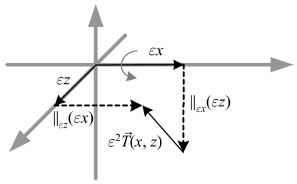
Figure 3.4: An example of non-zero torsion suggestive of spin.

The zero torsion expression $[v,w]=\nabla_{v}w-\nabla_{w}v$ means that we can replace partial with covariant derivatives in the usual expression for the Lie derivative of a vector field:

$$\left(L_{v}w\right)^{a} =\left[v,w\right]^{a}$$ (3.26)

$$=v^{b}\partial_{b}w^{a}-w^{b}\partial_{b}v^{a}$$

$$\overset{\cancel{T}}{=}v^{b}\nabla_{b}w^{a}-w^{b}\nabla_{b}v^{a}$$

This can be extended to the Lie derivative of a general tensor, so that in the case of zero torsion we have

$$L_{v}?T^{a_{1}\dots a_{m}}{}_{b_{1}\dots b_{n}}? =v^{c}\nabla_{c}?T^{a_{1}\dots a_{m}}{}_{b_{1}\dots b_{n}}?$$ (3.27)

$$-\sum_{j=1}^{m}\left(\nabla_{c}v^{a_{j}}\right)?T^{a_{1}\dots a_{j-1}ca_{j+1}\dots a_{m}}{}_{b_{1}\dots b_{n}}?$$

$$+\sum_{j=1}^{n}\left(\nabla_{b_{j}}v^{c}\right)?T^{a_{1}\dots a_{m}}{}_{b_{1}\dots b_{j-1}cb_{j+1}\dots b_{n}}?.$$

3.5 Curvature

The exterior covariant derivative $\mathrm{D}$ parallel transports its values on the boundary before summing them, and therefore we do not expect it to mimic the property $\mathrm{d}^{2}=0$ (see Section C.4). Indeed it does not; instead, for a vector field $w$ viewed as a vector-valued 0-form $\vec{w}$, we have

$$\left(\mathrm{D}^{2}\vec{w}\right)(u,v)\equiv\check{R}\left(u,v\right)\vec{w}=\nabla_{u}\nabla_{v}w-\nabla_{v}\nabla_{u}w-\nabla_{\left[u,v\right]}w,$$ (3.28)

which defines the curvature 2-form $\check{R}$, which is $gl(\mathbb{R}^{n})$-valued. From its definition, $\check{R}\vec{w}$ is a frame-independent quantity, and thus if $\vec{w}$ is considered as a vector-valued 0-form, $\check{R}$ is frame-independent as well. In the (more common) case that we view $\vec{w}$ as a frame-dependent $\mathbb{R}^{n}$-valued 0-form, $\check{R}$ must be considered to be $gl(n,\mathbb{R})$-valued, and is thus a frame-dependent matrix. A connection with zero curvature is called flat, as is any region of $M$ with a flat connection.

For a general $\mathbb{R}^{n}$-valued form $\vec{\varphi}$ it is not hard to arrive at an expression for $\check{R}$ in terms of the connection:

$$\mathrm{D}^{2}\vec{\varphi}=\left(\mathrm{d}\check{\Gamma}+\check{\Gamma}\wedge\check{\Gamma}\right)\wedge\vec{\varphi}\equiv\check{R}\wedge\vec{\varphi}$$ (3.29)

Note that $\mathrm{D}\check{\Gamma}=\mathrm{d}\check{\Gamma}+\check{\Gamma}[\wedge]\check{\Gamma}$ is a similar but distinct construction, since e.g.

$$(\check{\Gamma}\wedge\check{\Gamma})\left(v,w\right)=\check{\Gamma}\left(v\right)\check{\Gamma}\left(w\right)-\check{\Gamma}\left(w\right)\check{\Gamma}\left(v\right),$$ (3.30)

while

$$(\check{\Gamma}[\wedge]\check{\Gamma})\left(v,w\right) =[\check{\Gamma}\left(v\right),\check{\Gamma}\left(w\right)]-[\check{\Gamma}\left(w\right),\check{\Gamma}\left(v\right)]$$ (3.31)

$$=2(\check{\Gamma}\wedge\check{\Gamma})\left(v,w\right).$$

Thus we have

$$\check{R} \equiv\mathrm{d}\check{\Gamma}+\check{\Gamma}\wedge\check{\Gamma}$$ (3.32)

$$=\mathrm{d}\check{\Gamma}+\frac{1}{2}\check{\Gamma}[\wedge]\check{\Gamma}.$$

The definition of $\check{R}$ in terms of $\check{\Gamma}$ is sometimes called Cartan’s second structure equation. An immediate property from the definition of $\check{R}$ is

$$\check{R}(u,v)=-\check{R}(v,u),$$ (3.33)

which allows us to write e.g. for a vector-valued 1-form $\vec{\varphi}$

$$\left(\mathrm{D}^{2}\vec{\varphi}\right)(u,v,w) \equiv\left(\check{R}\wedge\vec{\varphi}\right)\left(u,v,w\right)$$ (3.34)

$$=\check{R}\left(u,v\right)\vec{\varphi}(w)+\check{R}\left(v,w\right)\vec{\varphi}(u)+\check{R}\left(w,u\right)\vec{\varphi}(v).$$

Constructing the same picture as can be done for the double exterior derivative (see Section C.4), we put

$$\mathrm{D}^{2}\vec{w}\equiv\mathrm{D}\vec{\varphi},$$

where

$$\vec{\varphi}(v)\equiv\mathrm{D}\vec{w}(v)=\nabla_{v}w.$$

Expanding both derivatives in terms of parallel transport, we find in the following figure that as we sum values around the boundary of the surface defined by its arguments, $\mathrm{D}^{2}$ fails to cancel the endpoint and starting point at the far corner. Examining the values of these non-canceling points, we can view the curvature as “the difference between $w$ when parallel transported around the two opposite edges of the boundary of the surface defined by its arguments.”

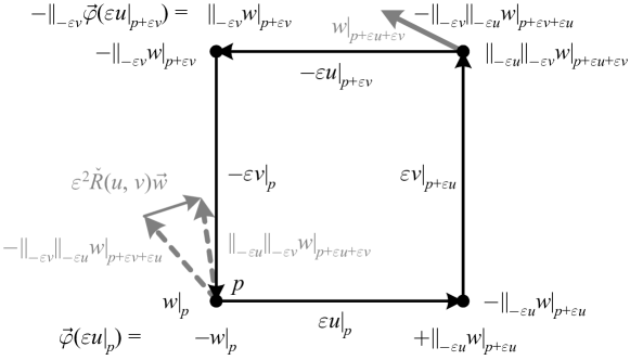
Figure 3.5: $\check{R}\left(u,v\right)\vec{w}=\left(\mathrm{D}^{2}\vec{w}\right)(u,v)$ is “the difference between $w$ when parallel transported around the two opposite edges of the boundary of the surface defined by its arguments.” In the figure we assume vanishing Lie bracket for simplicity, so that $v\left|{}_{p+\varepsilon u+\varepsilon v}\right.=v\left|{}_{p+\varepsilon v+\varepsilon u}\right.$.

In terms of the connection, we can use the path integral formulation to examine the parallel transporter around the closed path $L\equiv\partial S$ defined by the surface $S\equiv\left(\varepsilon u\wedge\varepsilon v\right)$ to order $\varepsilon^{2}$. This calculation after some work (see [4] pp. 51-53) yields

$$\parallel_{L}(w) =P\textrm{exp}\left(-\int_{L}\check{\Gamma}\right)\vec{w}$$ (3.35)

$$=w-\int_{S}\left(\mathrm{d}\check{\Gamma}+\check{\Gamma}\wedge\check{\Gamma}\right)\vec{w}$$

$$=w-\varepsilon^{2}\check{R}\left(u,v\right)\vec{w},$$

where we have dropped the indices since $L$ is a closed path and thus $\parallel_{L}$ is basis-independent. Thus the curvature can be viewed as “the difference between $w$ and its parallel transport around the boundary of the surface defined by its arguments.”

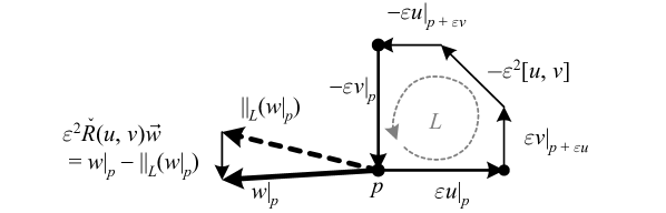
Figure 3.6: $\check{R}\left(u,v\right)\vec{w}$ is “the difference between $w$ and its parallel transport around the boundary of the surface defined by its arguments.”

As this picture suggests, one can verify algebraically that the value of $\check{R}\left(u,v\right)\vec{w}$ at a point $p$ only depends upon the value of $w$ at $p$, even though it can be defined in terms of $\nabla w$, which depends upon nearby values of $w$. Similarly, $\check{R}\left(u,v\right)\vec{w}$ at a point $p$ only depends upon the values of $u$ and $v$ at $p$, even though it can be defined in terms of $[u,v]$, which depends upon their vector field values (note that $\nabla_{u}\nabla_{v}w$ depends upon the vector field values of both $v$ and $w$). Finally, $\check{R}$ (as a $gl(\mathbb{R}^{n})$-valued 2-form) is frame-independent, even though it can be defined in terms of $\check{\Gamma}$, which is not. Thus the curvature can be viewed as a tensor of type $\left(1,3\right)$, called the Riemann curvature tensor (AKA Riemann tensor, curvature tensor, Riemann–Christoffel tensor):

$$?R^{c}{}_{dab}?u^{a}v^{b}w^{d} \equiv u^{a}\nabla_{a}\left(v^{b}\nabla_{b}w^{c}\right)-v^{b}\nabla_{b}\left(u^{a}\nabla_{a}w^{c}\right)-[u,v]^{d}\nabla_{d}w^{c}$$ (3.36)

$$=u^{a}v^{b}\nabla_{a}\nabla_{b}w^{c}-u^{a}v^{b}\nabla_{b}\nabla_{a}w^{c}+?T^{d}{}_{ab}?u^{a}v^{b}\nabla_{d}w^{c}$$

$$\Rightarrow?R^{c}{}_{dab}?w^{d} =\left(\nabla_{a}\nabla_{b}-\nabla_{b}\nabla_{a}+?T^{d}{}_{ab}?\nabla_{d}\right)w^{c}$$

Here we have used the Leibniz rule and recalled that $[u,v]^{d}=u^{a}\nabla_{a}v^{d}-v^{b}\nabla_{b}u^{d}-?T^{d}{}_{ab}?u^{a}v^{b}$.

To obtain an expression in terms of the connection coefficients, we first examine the double covariant derivative, recalling that $\nabla_{b}w^{c}$ is a tensor:

$$\nabla_{a}\left(\nabla_{b}w^{c}\right) =\partial_{a}\nabla_{b}w^{c}+\Gamma^{c}{}_{fa}\nabla_{b}w^{f}-\Gamma^{f}{}_{ba}\nabla_{f}w^{c}$$ (3.37)

$$=\partial_{a}\partial_{b}w^{c}+\partial_{a}(\Gamma^{c}{}_{fb}w^{f})$$

$$\phantom{{}=}+\Gamma^{c}{}_{fa}\partial_{b}w^{f}+\Gamma^{c}{}_{fa}\Gamma^{f}{}_{gb}w^{g}-\Gamma^{f}{}_{ba}\nabla_{f}w^{c}$$

$$=\partial_{a}\partial_{b}w^{c}+\partial_{a}\Gamma^{c}{}_{fb}w^{f}$$

$$\phantom{{}=}+\Gamma^{c}{}_{fb}\partial_{a}w^{f}+\Gamma^{c}{}_{fa}\partial_{b}w^{f}$$

$$\phantom{{}=}+\Gamma^{c}{}_{fa}\Gamma^{f}{}_{gb}w^{g}-\Gamma^{f}{}_{ba}\nabla_{f}w^{c}.$$

When we subtract the same expression with $a$ and $b$ reversed, we recognize that for the functions $w^{c}$ we have $\partial_{a}\partial_{b}w^{c}-\partial_{b}\partial_{a}w^{c}=[e_{a},e_{b}]^{d}\partial_{d}w^{c}$, that the second line $\Gamma^{c}{}_{fb}\partial_{a}w^{f}+\Gamma^{c}{}_{fa}\partial_{b}w^{f}$ vanishes, and that $\Gamma^{f}{}_{ba}-\Gamma^{f}{}_{ab}=[e_{a},e_{b}]^{f}+?T^{f}{}_{ab}?$, so that

$$\left(\nabla_{a}\nabla_{b}-\nabla_{b}\nabla_{a}\right)w^{c} =[e_{a},e_{b}]^{d}\partial_{d}w^{c}+\partial_{a}\Gamma^{c}{}_{fb}w^{f}-\partial_{b}\Gamma^{c}{}_{fa}w^{f}$$ (3.38)

$$\phantom{{}=}+\Gamma^{c}{}_{fa}\Gamma^{f}{}_{gb}w^{g}-\Gamma^{c}{}_{fb}\Gamma^{f}{}_{ga}w^{g}$$

$$\phantom{{}=}-\left([e_{a},e_{b}]^{f}+?T^{f}{}_{ab}?\right)\nabla_{f}w^{c},$$

and thus relabeling dummy indices to obtain an expression in terms of $w^{d}$, we arrive at

$$?R^{c}{}_{dab}?w^{d} =\left(\nabla_{a}\nabla_{b}-\nabla_{b}\nabla_{a}+?T^{d}{}_{ab}?\nabla_{d}\right)w^{c}$$ (3.39)

$$=\left(\partial_{a}\Gamma^{c}{}_{db}-\partial_{b}\Gamma^{c}{}_{da}+\Gamma^{c}{}_{fa}\Gamma^{f}{}_{db}-\Gamma^{c}{}_{fb}\Gamma^{f}{}_{da}-[e_{a},e_{b}]^{f}\Gamma^{c}{}_{df}\right)w^{d}.$$

This expression follows much more directly from the expression $\check{R}\equiv\mathrm{d}\check{\Gamma}+\check{\Gamma}\wedge\check{\Gamma}$, but the above derivation from the covariant derivative expression is included here to clarify other presentations which are sometimes obscured by the quirks of index notation for covariant derivatives.

$\triangle$ The derivation above makes clear how the expression for the curvature in terms of the covariant derivative simplifies to $?R^{c}{}_{dab}?w^{d}=\left(\nabla_{a}\nabla_{b}-\nabla_{b}\nabla_{a}\right)w^{c}$ for zero torsion but is unchanged in a holonomic frame, while in contrast the expression in terms of the connection coefficients is unchanged for zero torsion but in a holonomic frame simplifies to omit the term $[e_{a},e_{b}]^{f}\Gamma^{c}{}_{df}w^{d}$.

$\triangle$ Note that the sign and the order of indices of $R$ as a tensor are not at all consistent across the literature.

3.6 First Bianchi identity

If we take the exterior covariant derivative of the torsion, we get

$$\mathrm{D}\vec{T}=\mathrm{DD}\vec{\beta}=\check{R}\wedge\vec{\beta}.$$ (3.40)

This is called the first (AKA algebraic) Bianchi identity. Using the antisymmetry of $\check{R}$, we can write the first Bianchi identity explicitly as

$$\mathrm{D}\vec{T}(u,v,w)=\check{R}(u,v)\vec{w}+\check{R}(v,w)\vec{u}+\check{R}(w,u)\vec{v}.$$ (3.41)

In the case of zero torsion, this identity becomes $\check{R}\wedge\vec{\beta}=0$, which in index notation can be written $?R^{c}{}_{[dab]}?=0$.

We can find a geometric interpretation for this identity by first constructing a variant of our picture of $\check{R}(u,v)\vec{w}$ as the change in $\vec{w}$ after being parallel transported in opposite directions around a loop. Taking advantage of our previous result that $\check{R}(u,v)\vec{w}$ only depends upon the local values of $u$ and $v$, we are free to construct their vector field values such that $[u,v]=0$. We then examine the difference between $\vec{w}$ being parallel transported in each direction halfway around the loop. For infinitesimal parallel transport from a point $p$ along a curve $C$ with tangent $v$ we have $\parallel_{\varepsilon v}(w\left|{}_{p}\right.)\equiv\parallel_{C}(w\left|{}_{p}\right.)=w\left|{}_{p+\varepsilon v}\right.-\varepsilon\nabla_{v}w\left|{}_{p}\right.$. Therefore we find that

$$\parallel_{\varepsilon u}\parallel_{\varepsilon v}(w\left|{}_{p}\right.) =\parallel_{u}\left(w\left|{}_{p+\varepsilon v}\right.-\varepsilon\nabla_{v}w\left|{}_{p}\right.\right)$$ (3.42)

$$=w\left|{}_{p+\varepsilon v+\varepsilon u}\right.-\varepsilon\nabla_{v}w\left|{}_{p+\varepsilon u}-\varepsilon\nabla_{u}w\left|{}_{p+\varepsilon v}\right.+\varepsilon^{2}\nabla_{u}\nabla_{v}w\left|{}_{p},\right.\right.$$

so that

$$\parallel_{\varepsilon u}\parallel_{\varepsilon v}(w\left|{}_{p}\right.)-\parallel_{\varepsilon v}\parallel_{\varepsilon u}(w\left|{}_{p}\right.) =\varepsilon^{2}\nabla_{u}\nabla_{v}w\left|{}_{p}\right.-\varepsilon^{2}\nabla_{v}\nabla_{u}w\left|{}_{p}\right.$$ (3.43)

$$=\varepsilon^{2}\check{R}(u,v)\vec{w},$$

since $[u,v]=0$ means that $w\left|{}_{p+\varepsilon v+\varepsilon u}\right.=w\left|{}_{p+\varepsilon u+\varepsilon v}\right.$. In the case of zero torsion, we can further take advantage of our freedom in choosing the vector field values of $u$ and $v$ by requiring them to equal their parallel transports, i.e. $v\left|{}_{p+\varepsilon u}\right.\equiv\parallel_{\varepsilon u}(v\left|{}_{p}\right.)$ and $u\left|{}_{p+\varepsilon v}\right.\equiv\parallel_{\varepsilon v}(u\left|{}_{p}\right.)$, preserving the property $[u,v]=0$ due to the vanishing torsion.

Figure 3.7: A slight variant of $\check{R}\left(u,v\right)\vec{w}$ viewed as “the difference between $w$ when parallel transported around the two opposite edges of the boundary of the surface defined by its arguments.” In the case of zero torsion, the boundary can be built from parallel transports instead of vector field values.

Thus, still assuming zero torsion, we can construct a cube from the parallel transports of $u$, $v$, and $w$. This construction reveals that the first Bianchi identity corresponds to the fact that the three curvature vectors form a triangle, i.e. their sum is zero.

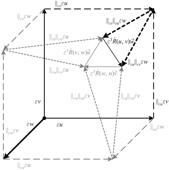
Figure 3.8: The first Bianchi identity reflects the fact that for zero torsion, the far corners of a cube made of parallel transported vectors do not meet, and their separation is made up of the differences in parallel transport via opposite edges of each face. Note that the corners of the triangle are points since vanishing torsion means that e.g. $\varepsilon u+\parallel_{\varepsilon u}(\varepsilon w)=\varepsilon w+\parallel_{\varepsilon w}(\varepsilon u)$, so that the top point of the triangle reflects this equality parallel transported by $\varepsilon v$.

3.7 Second Bianchi identity

If we take the exterior covariant derivative of the curvature, we get

$$\mathrm{D}\check{R}=0.$$ (3.44)

This is called the second Bianchi identity, and can be verified algebraically from the definition $\check{R}\equiv\mathrm{d}\check{\Gamma}+\check{\Gamma}\wedge\check{\Gamma}$. We can write this identity more explicitly as

$$0 =\mathrm{D}\check{R}(u,v,w)\vec{a}$$ (3.45)

$$=\nabla_{u}\check{R}(v,w)\vec{a}+\nabla_{v}\check{R}(w,u)\vec{a}+\nabla_{w}\check{R}(u,v)\vec{a}$$

$$\phantom{{}=}-\check{R}([u,v],w)\vec{a}-\check{R}([v,w],u)\vec{a}-\check{R}([w,u],v)\vec{a},$$

where we have used the antisymmetry of $\check{R}$ and the covariant derivative acts on the value of $\check{R}$ as a tensor of type $\left(1,1\right)$. Working this expression into tensor notation and using the tensor expression for the torsion in terms of the commutator, we find that

$$0 =\nabla_{e}?R^{c}{}_{dab}?+\nabla_{a}?R^{c}{}_{dbe}?+\nabla_{b}?R^{c}{}_{dea}?$$ (3.46)

$$\phantom{{}=}-?R^{c}{}_{dfe}??T^{f}{}_{ab}?-?R^{c}{}_{dfa}??T^{f}{}_{be}?-?R^{c}{}_{dfb}??T^{f}{}_{ea}?,$$

or

$$?R^{c}{}_{d[ab;e]}?=?R^{c}{}_{df[e}??T^{f}{}_{ab]}?,$$ (3.47)

and in the case of zero torsion, $?R^{c}{}_{d[ab;e]}?=0$.

Geometrically, the second Bianchi identity can be seen as reflecting the same “boundary of a boundary” idea as that of $\mathrm{d}^{2}=0$ in Fig. C.8, except that here we are parallel transporting a vector $\vec{a}$ around each face that makes up the boundary of the cube. As in the previous section, we can take advantage of the fact that $\check{R}(v,w)\vec{a}$ only depends upon the local value of $\vec{a}$, constructing its vector field values such that e.g. $\vec{a}\left|{}_{p+\varepsilon u}\right.=\parallel_{\varepsilon u}(\vec{a}\left|{}_{p}\right.)$, giving us

$$\varepsilon\nabla_{u}\check{R}(v,w)\vec{a} =\check{R}(v\left|{}_{p+\varepsilon u}\right.,w\left|{}_{p+\varepsilon u}\right.)\vec{a}\left|{}_{p+\varepsilon u}\right.-\parallel_{\varepsilon u}\check{R}(v,w)\parallel_{\varepsilon u}^{-1}\vec{a}\left|{}_{p+\varepsilon u}\right.$$ (3.48)

$$=\check{R}(v\left|{}_{p+\varepsilon u}\right.,w\left|{}_{p+\varepsilon u}\right.)\parallel_{\varepsilon u}\vec{a}-\parallel_{\varepsilon u}\check{R}(v,w)\vec{a}.$$

The first term parallel transports $\vec{a}$ along $\varepsilon u$ and then around the parallelogram defined by $v$ and $w$ at $p+\varepsilon u$, while the second parallel transports $\vec{a}$ around the parallelogram defined by $v$ and $w$ at $p$, then along $\varepsilon u$. Thus in the case of vanishing Lie commutators (e.g. a holonomic frame), we construct a cube from the vector fields $u$, $v$, and $w$, and find that the second Bianchi identity reflects the fact that $\mathrm{D}\check{R}(u,v,w)\vec{a}$ parallel transports $\vec{a}$ along each edge of the cube an equal number of times in opposite directions, thus canceling out any changes.

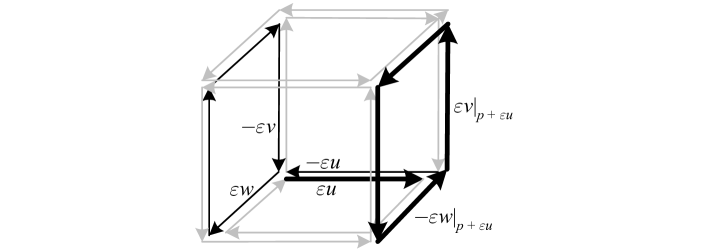
Figure 3.9: The second Bianchi identity reflects the fact that for vanishing Lie commutators, $\mathrm{D}\check{R}(u,v,w)\vec{a}$ parallel transports $\vec{a}$ along each edge of the cube made of the three vector field arguments an equal number of times in opposite directions, thus canceling out any changes. Above, $\varepsilon\nabla_{u}\check{R}(v,w)\vec{a}=\check{R}(v\left|{}_{p+\varepsilon u}\right.,w\left|{}_{p+\varepsilon u}\right.)\parallel_{\varepsilon u}\vec{a}-\parallel_{\varepsilon u}\check{R}(v,w)\vec{a}$ is highlighted by the bold arrows representing the path along which $\vec{a}$ is parallel transported in the first term, and by the remaining dark arrows representing the path along which $\vec{a}$ is parallel transported in the second term.

In the case of non-vanishing torsion, where there is a non-vanishing commutator $\vec{T}(u,v)=-[u,v]\neq 0$, we find that the cube gains a “shaved edge,” and that the extra non-vanishing term $-\check{R}([u,v],w)\vec{a}$ in $\mathrm{D}\check{R}$ maintains the “boundary of a boundary” logic by adding a loop of parallel transports of $\vec{a}$ in the proper direction around the new “face” created.

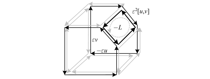
Figure 3.10: In the case of non-vanishing torsion and thus commutator, the extra term $-\check{R}([u,v],w)\vec{a}$ in $\mathrm{D}\check{R}$ maintains the cancellation of face boundaries by adding a loop $L$ around the new “shaved edge” created.

4 Introducing the metric

4.1 The Riemannian metric

A (pseudo) metric tensor (see Section A.4) is a (pseudo) inner product $\left\langle v,w\right\rangle$ on a vector space $V$ that can be represented by a symmetric tensor $g_{ab}$, and thus can be used to lower and raise indices on tensors. A (pseudo) Riemannian metric (AKA metric) is a (pseudo) metric tensor field on a manifold $M$, making $M$ a (pseudo) Riemannian manifold.

A metric defines the length (norm) of tangent vectors, and can thus be used to define the length $L$ of a curve $C$ via parametrization and integration:

$$L(C) \equiv\int\left\|\dot{C}(t)\right\|\mathrm{d}t$$ (4.1)

$$=\int\sqrt{\left\langle\dot{C}(t),\dot{C}(t)\right\rangle}\mathrm{d}t$$

This also turns any (non-pseudo) Riemannian manifold into a metric space, with distance function $d(x,y)$ defined to be the minimum length curve connecting the two points $x$ and $y$; this curve is called a (Riemannian) geodesic, and it locally minimizes the distance between any of its points. With a pseudo-Riemannian metric the distance may be instead maximized, and this extremal distance is only locally valid since e.g. the curve may eventually self-intersect as the equator on a sphere does. It can be shown that for any tangent vector $v$ on a Riemannian manifold there is a unique geodesic $C_{v}(d)$ parametrized by distance whose tangent is $v$; one can then define the exponential map by $\mathrm{exp}(v)\equiv C_{v}(1)$.

☼ With a metric, our intuitive picture of a manifold loses its “stretchiness” via the introduction of length and angles; but having only intrinsically defined properties, the manifold can still be e.g. rolled up like a piece of paper if imagined as flat and embedded in a larger space.

If the coordinate frame of $x^{\mu}$ is orthonormal at a point $p\in M^{n}$ in a Riemannian manifold, for arbitrary coordinates $y^{\mu}$ we can consider the components of the metric tensor in the two coordinate frames to find that

$$g_{\mu\nu}\mathrm{d}y^{\mu}\mathrm{d}y^{\nu} =\delta_{\lambda\sigma}\mathrm{d}x^{\lambda}\mathrm{d}x^{\sigma}$$ (4.2)

$$=\delta_{\lambda\sigma}\frac{\partial x^{\lambda}}{\partial y^{\mu}}\mathrm{d}y^{\mu}\frac{\partial x^{\sigma}}{\partial y^{\nu}}\mathrm{d}y^{\nu}$$

$$=\left[J_{x}(y)\right]^{T}\left[J_{x}(y)\right]\mathrm{d}y^{\mu}\mathrm{d}y^{\nu}$$

$$\Rightarrow\mathrm{det}\left(g_{\mu\nu}\right) =\left[\mathrm{det}\left(J_{x}\left(y\right)\right)\right]^{2},$$

where $J_{x}(y)$ is the Jacobian matrix (see Section B.6) and we have used the fact that $\mathrm{det}(A^{T}A)=[\mathrm{det}(A)]^{2}$. Thus the volume of an region $U\in M^{n}$ corresponding to $R\in\mathbb{R}^{n}$ in the coordinates $x^{\mu}$ is

$$V(U)=\int_{R}\sqrt{\mathrm{det}(g)}\mathrm{d}x^{1}\ldots\mathrm{d}x^{n},$$ (4.3)

where $\mathrm{det}(g)$ is the determinant of the metric tensor as a matrix in the coordinate frame $\partial/\partial x^{\mu}$. In the context of a pseudo-Riemannian manifold $\mathrm{det}(g)$ can be negative, and the integrand

$$\mathrm{d}V\equiv\sqrt{\left|\mathrm{det}(g)\right|}\mathrm{d}x^{1}\ldots\mathrm{d}x^{n}$$ (4.4)

is called the volume element, or when written as a form $\mathrm{d}V\equiv\sqrt{\left|\mathrm{det}(g)\right|}\mathrm{d}x^{1}\wedge\cdots\wedge\mathrm{d}x^{n}$ it is called the volume form. In physical applications $\mathrm{d}V$ usually denotes the volume pseudo-form, which gives a positive value regardless of orientation. Note that if the coordinate basis is orthonormal then $\left|\mathrm{det}(g)\right|=1$; thus these definitions are consistent with those typically defined on $\mathbb{R}^{n}$. Sometimes one defines a volume form on a manifold without defining a metric; in this case the metric (and connection) is not uniquely determined.

$\triangle$ The symbol $g$ is frequently used to denote $\mathrm{det}(g)$, and sometimes $\sqrt{\left|\mathrm{det}(g)\right|}$, in addition to denoting the metric tensor itself.

We can use the inner product to define an orthonormal frame on $M$. In four dimensions an orthonormal frame is also called a tetrad (AKA vierbein). Any frame on a manifold can be defined to be an orthonormal frame, which is equivalent to defining the metric (which in the orthonormal frame is $g_{ab}=\eta_{ab}$). An orthonormal holonomic frame exists on a region of $M$ if and only if that region is flat. Thus in general, given a set of coordinates on $M$, we have to choose between using either a non-coordinate orthonormal frame or a non-orthonormal coordinate frame.

The Hopf-Rinow theorem says that a connected Riemannian manifold $M$ is complete as a metric space (or equivalently, all closed and bounded subsets are compact) if and only if it is geodesically complete, meaning that the exponential map is defined for all vectors at some $p\in M$. If $M$ is geodesically complete at $p$, then it is at all points on the manifold, so this property can also be used to state the theorem. This theorem is not valid for pseudo-Riemannian manifolds; any (pseudo) Riemannian manifold that is geodesically complete is called a geodesic manifold.

As noted previously, a Riemannian metric can be defined on any differentiable manifold. In general, not every manifold admits a pseudo-Riemannian metric, and in particular not every 4-manifold admits a Minkowski metric, but 4-manifolds that are noncompact, parallelizable, or compact, connected and of Euler characteristic 0 all do.

In the same way that differentiable manifolds are equivalent if they are related by a diffeomorphism, Riemannian manifolds are equivalent if they are related by an isometry, a diffeomorphism $\Phi\colon M\to N$ that preserves the metric, i.e. $\forall v,w\in TM$, $\left\langle v,w\right\rangle\left|{}_{p}\right.=\left\langle\mathrm{d}\Phi_{p}(v),\mathrm{d}\Phi_{p}(w)\right\rangle\left|{}_{\Phi(p)}\right.$. Also like diffeomorphisms, the isometries of a manifold form a group; for example, the group of isometries of Minkowski space is the Poincaré group. A vector field whose one-parameter diffeomorphisms are isometries is called a Killing field, also called a Killing vector since it can be shown ([8] pp. 188-189) that a Killing field is determined by a vector at a single point along with its covariant derivatives. A Killing field thus satisfies $L_{v}g_{ab}=0$, which using eq. (3.27) for a Levi-Civita connection (see next section) is equivalent to

$$\nabla_{a}v_{b}+\nabla_{b}v_{a}=0,$$ (4.5)

called the Killing equation (AKA Killing condition).

We can then consider isometric immersions and embeddings, and ask whether every Riemannian manifold can be embedded in some $\mathbb{R}^{n}$. The Nash embedding theorem provides an affirmative answer, and it can also be shown that every pseudo-Riemannian manifold can be isometrically embedded in some $\mathbb{R}^{n}$ with some signature while maintaining arbitrary differentiability of the metric.

4.2 The Levi-Civita connection

A connection on a Riemannian manifold $M$ is called a metric connection (AKA metric compatible connection, isometric connection) if its associated parallel transport respects the metric, i.e. it preserves lengths and angles. More precisely, $\forall v,w\in TM$, we require that

$$\left\langle\parallel_{C}(v),\parallel_{C}(w)\right\rangle=\left\langle v,w\right\rangle$$ (4.6)

for any curve $C$ in $M$.

In terms of the metric, this can be written $g_{ab}\parallel_{C}v^{a}\parallel_{C}w^{b}=g_{ab}v^{a}w^{b}$. But recalling that the parallel transport of tensors just transports the arguments, we also have $\left(\parallel_{-C}g_{ab}\right)v^{a}w^{b}=g_{ab}\parallel_{C}v^{a}\parallel_{C}w^{b}$, so that we must have $\parallel_{-C}g_{ab}=g_{ab}$, or $\nabla_{c}g_{ab}=0$. Using the Leibniz rule for the covariant derivative over the tensor product, we can derive a Leibniz rule over the inner product:

$$\nabla_{c}\left(g_{ab}v^{a}w^{b}\right) =0+g_{ab}\nabla_{c}v^{a}w^{b}+g_{ab}v^{a}\nabla_{c}w^{b}$$ (4.7)

$$\Rightarrow\nabla_{u}\left\langle v,w\right\rangle =\left\langle\nabla_{u}v,w\right\rangle+\left\langle v,\nabla_{u}w\right\rangle$$

Requiring this relationship to hold is an equivalent way to define a metric connection. In terms of the connection coefficients, a metric connection then satisfies

$$\nabla_{c}g_{ab} =\partial_{c}g_{ab}-\Gamma^{d}{}_{ac}g_{db}-\Gamma^{d}{}_{bc}g_{ad}=0.$$ (4.8)

$$\Rightarrow\partial_{c}g_{ab} =\Gamma{}_{abc}+\Gamma{}_{bac},$$

where we write $\Gamma{}_{abc}\equiv\Gamma^{d}{}_{bc}g_{ad}$, which again it is important to note is not tensor. By considering $\partial_{c}\left(g^{ad}g_{df}\right)=\partial_{c}\left(\delta^{a}{}_{f}\right)=0$, we arrive at the complementary expression

$$\partial_{c}g^{ab} =-g^{ad}g^{bf}\partial_{c}g_{df}$$ (4.9)

$$=-\left(\Gamma^{ab}{}_{c}+\Gamma^{ba}{}_{c}\right).$$

The Levi-Civita connection (AKA Riemannian connection, Christoffel connection) is then the torsion-free metric connection on a (pseudo) Riemannian manifold $M$. The fundamental theorem of Riemannian geometry states that for any (pseudo) Riemannian manifold the Levi-Civita connection exists and is unique. On the other hand, an arbitrary connection can only be the Levi-Civita connection for some metric if it is torsion-free and preserves lengths; moreover, this metric is unique only up to a scaling factor (excepting special cases, e.g. if the manifold is a product space there can be a scaling factor for each factor space; in physics, this corresponds to a choice of units).

For a metric connection, the curvature then must take values that are infinitesimal rotations, i.e. $\check{R}$ is $o(r,s)$-valued. Thus if we eliminate the influence of the signature by lowering the first index, the first two indices of the curvature tensor are anti-symmetric:

$$R_{cdab}=-R{}_{dcab}$$ (4.10)

Using the anti-symmetry of the other indices and the first Bianchi identity, this leads to another commonly noted symmetry

$$R_{cdab}=R{}_{abcd}.$$ (4.11)

The Leibniz rule for the covariant derivative over the inner product along with the zero torsion relation $\nabla_{v}w=\nabla_{w}v+\left[v,w\right]$ can be used to derive an expression called the Koszul formula:

$$2\left\langle\nabla_{u}v,w\right\rangle= \nabla_{u}\left\langle v,w\right\rangle+\nabla_{v}\left\langle w,u\right\rangle-\nabla_{w}\left\langle u,v\right\rangle$$ (4.12)

$$-\left\langle u,[v,w]\right\rangle+\left\langle v,[w,u]\right\rangle+\left\langle w,[u,v]\right\rangle$$

Substituting in the frame vector fields and eliminating the metric tensor from the left hand side, we arrive at an expression for the connection in terms of the metric:

$$2\Gamma^{c}{}_{ba}=g^{cd}( \partial_{a}g_{bd}+\partial_{b}g_{da}-\partial_{d}g_{ab}$$ (4.13)

$$-g_{af}[e_{b},e_{d}]^{f}+g_{bf}[e_{d},e_{a}]^{f}+g_{df}[e_{a},e_{b}]^{f})$$

On a (pseudo) Riemannian manifold, the connection coefficients for the Levi-Civita connection in a coordinate basis $\Gamma^{\lambda}{}_{\mu\sigma}$ are called the Christoffel symbols, and are sometimes denoted $\{\begin{subarray}{c}\lambda\\ \mu\sigma\end{subarray}\}$ or $\{\begin{subarray}{c}\mu\sigma\\ \lambda\end{subarray}\}$. At a point $p\in U\subset M$, an orthonormal basis for $T_{p}U$ can be used to form geodesic normal coordinates, which are then called Riemann normal coordinates. Recalling from Section 2.6 that with zero torsion the connection coefficients vanish at $p$, we can apply the covariant derivative to the metric tensor to conclude that the partial derivatives of the metric $g_{\mu\nu}=\eta_{\mu\nu}$ all also vanish at $p$.

☼ The vanishing of the Christoffel symbols at the origin of Riemann normal coordinates is frequently used to simplify the derivation of tensor relations which are then, being frame-independent, seen to be true in any coordinate system or frame (and if the origin was chosen arbitrarily, at any point). In particular, the covariant and partial derivatives are equivalent at the origin of Riemann normal coordinates.

4.3 Independent quantities and dependencies

From their definitions, the parallel transport and connection in general determine each other. It can be shown that every manifold admits a connection, and every other connection can be obtained by adding a frame-independent $gl\left(\mathbb{R}^{n}\right)$-valued 1-form (tensor field of type $(1,2)$) to it. If the curvature is given over $M$, there is at most one metric (apart from special cases, up to a scaling factor, and for $n>2$) whose Levi-Civita connection yields this curvature.

If we choose coordinate charts and use coordinate frames on $M^{n}$, we can calculate the number of independent functions and equations associated with the various quantities and relations we have covered, and use them to verify the associated dependencies.

Quantity / relation	Viewpoint	Count
Metric	Symmetric matrix of functions	$n(n+1)/2$
Coordinate frame	Fixed	0
Connection	$gl$-valued (matrix-valued) 1-form	$n^{3}$
Metric condition	Derivative of metric	$n^{2}(n+1)/2$
Torsion-free condition	Vector-valued 2-form	$n^{2}(n-1)/2$

Table 4.1: Independent function and equation counts in a coordinate frame.

The choice of coordinates determines the frame, leaving the geometry of the Riemannian manifold defined by the $n(n+1)/2$ functions of the metric. A torsion-free connection consists of $n^{3}-n^{2}(n-1)/2=n^{2}(n+1)/2$ functions. The metric condition is exactly this number of equations, allowing us in general to solve for the connection if the metric is known, or vice-versa (up to a constant scaling factor).

Alternatively, we can look at things in a orthonormal frame:

Quantity / relation	Viewpoint	Count
Metric	Fixed	0
Orthonormal frame	$n$ vector fields	$n^{2}$
Change of orthonormal frame	$SO$-valued 0-form	$n(n-1)/2$
Connection	$so$-valued 1-form	$n^{2}(n-1)/2$
Metric condition	Automatically satisfied	0
Torsion-free condition	Vector-valued 2-form	$n^{2}(n-1)/2$

Table 4.2: Independent function and equation counts in an orthonormal frame.

Here the metric is fixed, defined by the frame, which consists of $n^{2}$ functions, but is determined only up to a change of orthonormal frame (rotation); this yields $n^{2}-n(n-1)/2=n(n+1)/2$ functions, consistent with the metric function count above. The torsion-free condition is the same number of equations as the connection has functions, so that in general the torsion-free connection can be determined by the orthonormal frame.

4.4 The divergence and conserved quantities

The divergence of a vector field $u$ (see Section C.5) can be generalized to a pseudo-Riemannian manifold of signature $\left(r,s\right)$ by defining

$$\mathrm{div}(u)\equiv(-1)^{s}*\mathrm{d}(*(u^{\flat})).$$ (4.14)

Using the relations $i_{u}\Omega=*(u^{\flat})$ (see Section C.6) and $(-1)^{s}A=(*A)\Omega$ for $A\in\Lambda^{n}M^{n}$ (see Section A.10), we have

$$\mathrm{d}(i_{u}\Omega) =\mathrm{d}(*(u^{\flat}))$$ (4.15)

$$=(-1)^{s}*\mathrm{d}(*(u^{\flat}))\Omega$$

$$=\mathrm{div}(u)\Omega.$$

Using $i_{u}\mathrm{d}+\mathrm{d}i_{u}=L_{u}$ we then arrive at $\mathrm{div}(u)\Omega=L_{u}\Omega$, or as it is more commonly written

$$\mathrm{div}(u)\mathrm{d}V=L_{u}\mathrm{d}V.$$ (4.16)

Thus we can say that $\mathrm{div}(u)$ is “the fraction by which a unit volume changes when transported by the flow of $u$,” and if $\mathrm{div}(u)=0$ then we can say that “the flow of $u$ leaves volumes unchanged.” Expanding the volume element in coordinates $x^{\lambda}$ we can obtain an expression for the divergence in terms of these coordinates,

$$\mathrm{div}(u)=\frac{1}{\sqrt{\left|\mathrm{det}(g)\right|}}\partial_{\lambda}\left(u^{\lambda}\sqrt{\left|\mathrm{det}(g)\right|}\right).$$ (4.17)

Note that both this metric-dependent expression and the expression $\nabla_{a}u^{a}$ (sometimes called the covariant divergence) in terms of the Levi-Civita connection are coordinate-independent and equal to $\partial_{a}u^{a}$ in Riemann normal coordinates, confirming our expectation that for zero torsion we have

$$\mathrm{div}(u)=\nabla_{a}u^{a}.$$ (4.18)

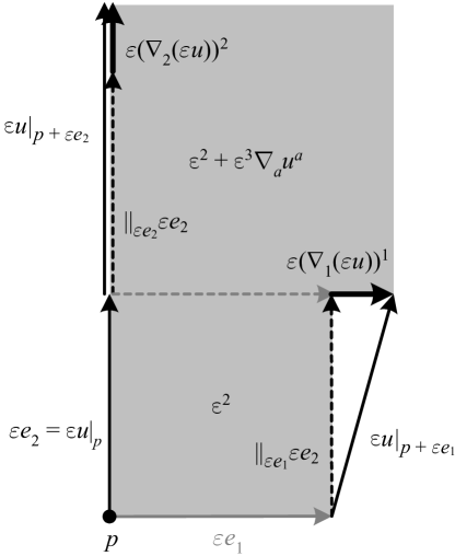
Figure 4.1: The divergence measures the change in volume due to the flow. Here we assume zero torsion, and that the vector field $u$ has unit length at point $p$, and choose an orthonormal frame which aligns $e_{2}$ with $u$. Each covariant derivative extends a face of the volume, with their sum being proportional to the total change in volume. Note that the upper right corner is of order $\varepsilon^{4}$ and so can be neglected, and e.g. any component of $\nabla_{1}u$ orthogonal to $e_{1}$ leaves the volume unchanged, since a more accurate depiction would include the volume with edge $-\varepsilon e_{1}$, where by linearity this component would be in the opposite direction and thus cancel the volume change. Also note that non-zero torsion would reduce the top edge $\parallel_{\varepsilon e_{2}}\varepsilon e_{1}$ by $\varepsilon^{2}?T^{1}{}_{1b}?u^{b}$, which must be added back by subtracting this component, matching the algebraic result.

Using the relation $\mathrm{div}(u)\Omega=\mathrm{d}(i_{u}\Omega)$ from eq. (4.15), along with Stokes’ theorem, we recover the classical divergence theorem

$$\int_{V}\mathrm{div}(u)\mathrm{d}V =\int_{\partial V}i_{u}\mathrm{d}V$$ (4.19)

$$=\int_{\partial V}\left\langle u,n\right\rangle\mathrm{d}S,$$

where $V$ is an $n$-dimensional compact submanifold of $M^{n}$, $n$ is the unit normal vector to $\partial V$, and $\mathrm{d}S\equiv i_{n}\mathrm{d}V$ is the induced volume element (“surface element”) for $\partial V$. In the case of a Riemannian metric, this can be thought of as reflecting the intuitive fact that “the change in a volume due to the flow of $u$ is equal to the net flow across that volume’s boundary.” If $\mathrm{div}(u)=0$ then we can say that “the net flow of $u$ across the boundary of a volume is zero.” We can also consider an infinitesimal $V$, so that the divergence at a point measures “the net flow of $u$ across the boundary of an infinitesimal volume.”

In physics, one considers the divergence of the current vector (AKA current density, flux, flux density) $j\equiv\rho u$ of a physical flow in space at a moment in time, where $\rho$ is the density of the physical quantity $Q$ and $u$ is thus a velocity field; e.g. in $\mathbb{R}^{3}$, $j$ has units $Q/(\mathrm{length})^{2}(\mathrm{time})$. For a flat Riemannian metric on the manifold representing space, the continuity equation (AKA equation of continuity) is

$$\frac{\mathrm{d}q}{\mathrm{d}t}=\Sigma-\int_{\partial V}\left\langle j,\hat{n}\right\rangle\mathrm{d}S,$$ (4.20)

where $q$ is the amount of $Q$ contained in $V$, $t$ is time, and $\Sigma$ is the rate of $Q$ being created within $V$. The continuity equation thus states the intuitive fact that the change of $Q$ within $V$ equals the amount generated less the amount which passes through $\partial V$.

Using the divergence theorem, we can then obtain the differential form of the continuity equation

$$\frac{\partial\rho}{\partial t}=\sigma-\mathrm{div}(j),$$ (4.21)

where $\sigma$ is the amount of $Q$ generated per unit volume per unit time. This equation then states the intuitive fact that at a point, the change in density of $Q$ equals the amount generated less the amount that moves away. Positive $\sigma$ is referred to as a source of $Q$, and negative $\sigma$ a sink. If $\sigma=0$ then we say that $Q$ is a conserved quantity and refer to the continuity equation as a (local) conservation law.

Under a flat Lorentzian metric, we can combine $\rho$ and $j$ into the four-current

$$J\equiv(\rho,j^{\mu}),$$ (4.22)

and express the continuity equation with $\sigma=0$ as

$$\mathrm{div}(J)=0,$$ (4.23)

whereupon $J$ is called a conserved current. Note that if any curvature is present (but no torsion), when we split out the time component we recover a Riemannian divergence but introduce a source due to the non-zero Christoffel symbols

$$\nabla_{\mu}J^{\mu} =\partial_{\mu}J^{\mu}+?\Gamma^{\mu}{}_{\nu\mu}?J^{\nu}$$ (4.24)

$$=\partial_{t}\rho+\nabla_{i}j^{i}+\left(?\Gamma^{\mu}{}_{t\mu}?\rho+?\Gamma^{t}{}_{it}?j^{i}\right),$$

where $t$ is the negative signature component and the index $i$ goes over the remaining positive signature components. Thus, since the Christoffel symbols are coordinate-dependent, in the presence of curvature there is in general no coordinate-independent conserved quantity associated with a vanishing Lorentzian divergence. A conserved current nevertheless means that the quantity is conserved in finite volumes of spacetime, in the sense that $\int_{\partial V}\left\langle J,\hat{n}\right\rangle\mathrm{d}S=0$ over any spacetime volume $V$, and the continuity equation holds for the components of the coordinate-dependent quantity $\mathfrak{J}\equiv J\sqrt{\left|\mathrm{det}(g)\right|}$, since

$$\partial_{\mu}\mathfrak{J}^{\mu} =\partial_{t}\mathfrak{J}^{t}+\partial_{i}\mathfrak{J}^{i}$$ (4.25)

$$=\partial_{t}\mathfrak{J}^{t}+\nabla_{i}\mathfrak{J}^{i}=0.$$

☼ Noether’s theorem derives conserved currents from transformations (“symmetries”) on the variables of an expression called the action that leave it unchanged.

4.5 Ricci and sectional curvature

The Ricci curvature tensor (AKA Ricci tensor) is formed by contracting two indices in the Riemann curvature tensor:

$$?R_{ab}? \equiv?R^{c}{}_{acb}?$$ (4.26)

$$\mathrm{Ric}(v,w) \equiv?R{}_{ab}?v^{a}w^{b}$$

Using the symmetries of the Riemann tensor for a metric connection along with the first Bianchi identity for zero torsion, it is easily shown that the Ricci tensor for the Levi-Civita connection is symmetric. A pseudo-Riemannian manifold is said to have constant Ricci curvature, or to be an Einstein manifold, if the Ricci tensor is a constant multiple of the metric tensor.

Since the Ricci tensor is symmetric for zero torsion, by the spectral theorem it can be diagonalized on a Riemannian manifold and thus is determined by

$$\mathrm{Ric}(v)\equiv\mathrm{Ric}(v,v),$$ (4.27)

which is called the Ricci curvature function (AKA Ricci function). Note that the Ricci function is not a 1-form since it is not linear in $v$. Choosing a basis that diagonalizes $R_{ab}$ is equivalent to choosing our basis vectors to line up with the directions that yield extremal values of the Ricci function on the unit vectors $\mathrm{Ric}(\hat{v},\hat{v})$ (or equivalently, the principal axes of the ellipsoid / hyperboloid $\mathrm{Ric}(v,v)=1$).

Finally, if we raise one of the indices of the Ricci tensor and contract we arrive at the Ricci scalar (AKA scalar curvature):

$$R \equiv g^{ab}R_{ab}$$ (4.28)

For a Riemannian manifold $M^{n}$, the Ricci scalar can thus be viewed as $n$ times the average of the Ricci function on the set of unit tangent vectors.

$\triangle$ The Ricci function and Ricci scalar are sometimes defined as averages instead of contractions (sums), introducing extra factors in terms of the dimension $n$ to the above definitions.

The Ricci function in terms of the curvature 2-form in an orthonormal frame $e_{\mu}$ (dropping the hats to avoid clutter) on a pseudo-Riemannian manifold $M^{n}$ naturally splits into terms which each also measure curvature:

$$\mathrm{Ric}(e_{\mu})=\sum_{i\neq\mu}g_{ii}\left\langle\check{R}(e_{i},e_{\mu})\vec{e}_{\mu},e_{i}\right\rangle$$ (4.29)

The term $i=\mu$ vanishes due to the anti-symmetry of $\check{R}$. The $(n-1)$ non-zero terms are each called a sectional curvature, which in general is defined as

$$K(v,w) \equiv\frac{\left\langle\check{R}(v,w)\vec{w},v\right\rangle}{\left\langle v,v\right\rangle\left\langle w,w\right\rangle-\left\langle v,w\right\rangle^{2}}$$ (4.30)

$$\Rightarrow K(e_{i},e_{j}) =g_{ii}g_{jj}\left\langle\check{R}(e_{i},e_{j})\vec{e}_{j},e_{i}\right\rangle$$

$$\Rightarrow\mathrm{Ric}(e_{\mu}) =\sum_{i\neq\mu}g_{\mu\mu}K(e_{i},e_{\mu})$$

$$\Rightarrow R =\sum_{j}g_{jj}\mathrm{Ric}(e_{j})$$

$$=\sum_{i\neq j}K(e_{i},e_{j})$$

$$=2\sum_{i<j}K(e_{i},e_{j}).$$

Note that the sectional curvature is not a 2-form since it is not linear in its arguments; in fact it is constructed to only depend on the plane defined by them, and therefore is symmetric and defined to vanish for equal arguments. Thus for a Riemannian manifold, the Ricci function of a unit vector $\mathrm{Ric}(\hat{v})$ can be viewed as $(n-1)$ times the average of the sectional curvatures of the planes that include $\hat{v}$, and the Ricci scalar can be viewed as $n$ times the average of all the Ricci functions. For a pseudo-Riemannian manifold, the Ricci scalar is twice the sum of all sectional curvatures, or $n(n-1)$ times the average of all sectional curvatures, whose count is the binomial coefficient $n$ choose 2 or $n(n-1)/2$.

The sectional curvatures completely determine the Riemann tensor, but in general the Ricci tensor alone does not for manifolds of dimension greater than 3. However, the Riemann tensor is determined by the Ricci tensor together with the Weyl curvature tensor (AKA Weyl tensor, conformal tensor), whose definition (not reproduced here) removes all contractions of the Riemann tensor, so that it is the “trace-free part of the curvature” (i.e. all of its contractions vanish). The Weyl tensor is only defined and non-zero for dimensions $n>3$.

The Einstein tensor is defined as

$$G(v,w) \equiv\mathrm{Ric}(v,w)-\frac{R}{2}g(v,w)$$ (4.31)

$$G_{ab} =R_{ab}-\frac{R}{2}g_{ab}.$$

If we define $G\equiv g^{ab}G_{ab}$ then we find that $R_{ab}=G_{ab}-Gg_{ab}/(n-2)$, so that the Einstein tensor vanishes iff the Ricci tensor does. Now, for zero torsion the Einstein tensor is symmetric, and by the spectral theorem can be diagonalized at a given point in an orthonormal basis, which also diagonalizes the Ricci tensor. In terms of the sectional curvature, we have

$$G(e_{\mu},e_{\mu}) =-g_{\mu\mu}\sum_{\begin{subarray}{c}i<j\\ i,j\neq\mu\end{subarray}}K(e_{i},e_{j}).$$ (4.32)

Thus for a Riemannian manifold, the Einstein tensor $G(\hat{v},\hat{v})$ applied to a unit vector twice can be viewed as $-\left\langle\hat{v},\hat{v}\right\rangle(n-1)(n-2)/2$ times the average of the sectional curvatures of the planes orthogonal to $\hat{v}$. Using the second Bianchi identity with zero torsion it can be shown ([3] pp. 80-81) that the Einstein tensor is also “divergenceless,” i.e.

$$\nabla_{a}G^{ab}=0.$$ (4.33)

For each value of $b$ in an orthonormal frame, this relation expressed in terms of the Riemann curvature tensor can be seen to be equivalent to the second Bianchi identity. Recall that unless the metric is flat, there is no conserved quantity which can be associated with this vanishing “divergence” for a Lorentzian metric.

$\triangle$ Frequent references to the divergencelessness of the Einstein tensor being related to a conserved quantity usually refer to some kind of particular context; one simple one is that in the limit of zero curvature or infinitesimal volume, there is a set of conserved quantities due to the above equation.

4.6 Curvature and geodesics

Geometrically, the Ricci function $\mathrm{Ric}(v)$ at a point $p\in M^{n}$ can be seen to measure the extent to which the area defined by the geodesics emanating from the $(n-1)$-surface perpendicular to $v$ changes in the direction of $v$. Considering the three dimensional case in an orthonormal frame (and again dropping the hats in $\hat{e}_{i}$ to avoid clutter), we have

$$\mathrm{Ric}(e_{2}) =\left\langle\check{R}(e_{1},e_{2})\vec{e}_{2},e_{1}\right\rangle+\left\langle\check{R}(e_{3},e_{2})\vec{e}_{2},e_{3}\right\rangle$$ (4.34)

$$=K(e_{1},e_{2})+K(e_{3},e_{2}).$$

If we form a cube made from parallel transported vectors as we did for the first Bianchi identity, we can see that each sectional curvature term in $\mathrm{Ric}(e_{2})$ takes an edge of the cube and measures the length of the difference between the cube-aligned component of its parallel transport in the $e_{2}$ direction and the edge of the cube at a point parallel transported in the $e_{2}$ direction.

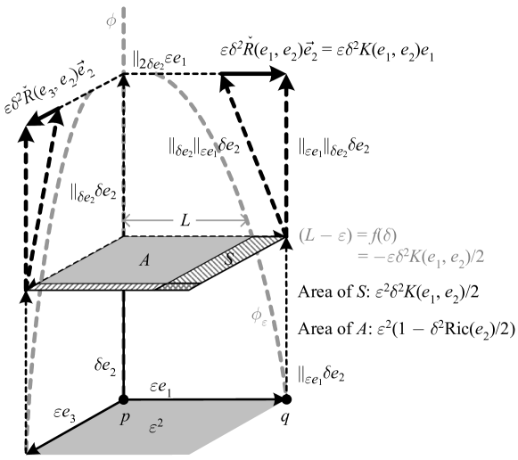
Figure 4.2: Each sectional curvature measures the convergence of geodesics, while their sum forms the Ricci curvature function, which measures the change in the area of the $(n-1)$-surface formed by geodesics perpendicular to its argument. In the figure we assume without loss of generality (see below) that $\check{R}(e_{1},e_{2})\vec{e}_{2}$ is parallel to $e_{1}$.

The figure above details the sectional curvature $K(e_{1},e_{2})=\beta^{1}\check{R}(e_{1},e_{2})\vec{e}_{2}$ assuming that $\check{R}(e_{1},e_{2})\vec{e}_{2}$ is parallel to $e_{1}$, so that $\left\langle\check{R}(e_{1},e_{2})\vec{e}_{2},e_{1}\right\rangle=\left\|\check{R}(e_{1},e_{2})\vec{e}_{2}\right\|$. The parallel transport of $e_{2}$ along itself is depicted as parallel, so that the geodesic parametrized by arclength $\phi(t)$ is a straight line in the figure. The vector $\parallel_{\delta e_{2}}\parallel_{\varepsilon e_{1}}\delta e_{2}$ is the parallel transport of $\parallel_{\varepsilon e_{1}}\delta e_{2}$ by $\delta$ in the direction parallel to $e_{2}$, and therefore the geodesic $\phi_{\varepsilon}(t)$ tangent to $\parallel_{\varepsilon e_{1}}\delta e_{2}$ at $q$ has tangent $\parallel_{\delta e_{2}}\parallel_{\varepsilon e_{1}}\delta e_{2}$ after moving a distance $\delta$. If we consider the function $f(t)$ whose value at $t=\delta$ is the quantity $(L-\varepsilon)$ in the figure (i.e. $f(t)$ measures the offset of the geodesic from the right edge of the stack of parallel cubes), its derivative is the slope of the tangent, so that to lowest order in $t$ we have

$$\dot{f}(t) =-\varepsilon t^{2}K(e_{1},e_{2})/t$$ (4.35)

$$=-\varepsilon tK(e_{1},e_{2})$$

$$\Rightarrow f(t) =-\varepsilon t^{2}K(e_{1},e_{2})/2.$$

We can generalize this logic to arbitrary unit vectors $\hat{v}$ and $\hat{w}$ to conclude that $K(\hat{v},\hat{w})/2$ is the “fraction by which the geodesic parallel to $\hat{w}$ with separation direction $\hat{v}$ bends towards $\hat{w}$.” More precisely, in terms of the distance function and the exponential map, to order $\varepsilon$ and $\delta^{2}$ we have

$$d\left(\mathrm{exp}(\delta\hat{w}),\mathrm{exp}(\delta\parallel_{\varepsilon\hat{v}}\hat{w})\right)=\varepsilon\left(1-\frac{\delta^{2}}{2}K(\hat{v},\hat{w})\right).$$ (4.36)

In the general case $L$ in the figure is the distance between two geodesics infinitesimally separated in the $\hat{v}$ direction, so if we define $L(t)$ as this distance at any point along the parametrized geodesic tangent to $\hat{w}$, the above becomes

$$L(t) =L(0)\left(1-\frac{t^{2}}{2}K(\hat{v},\hat{w})\right)$$ (4.37)

$$\Rightarrow\left.\frac{\ddot{L}}{L}\right|_{t=0} =-K(\hat{v},\hat{w}),$$

where the double dots indicate the second derivative with respect to $t$. Thus $K(\hat{v},\hat{w})$ is “the acceleration of two parallel geodesics in the $\hat{w}$ direction with initial separation $\hat{v}$ towards each other as a fraction of the initial gap.”

Now, the distance $\left|\varepsilon-L\right|=\varepsilon\delta^{2}K(e_{1},e_{2})/2$ defines a strip $S$ bordering the surface orthogonal to $e_{2}$ a distance $\delta$ in the $e_{2}$ direction. This strip thus has an area $\varepsilon^{2}\delta^{2}K(e_{1},e_{2})/2$. If we sum this with the other strip of area $\varepsilon^{2}\delta^{2}K(e_{3},e_{2})/2$, to order $\varepsilon^{2}$ and $\delta^{2}$ we measure the extent to which the area $A$ defined by the geodesics emanating from the surface perpendicular to $e_{2}$ changes in the direction of $e_{2}$. But the sum of sectional curvatures is just the Ricci function, so that in general $\mathrm{Ric}(v)/2$ is the “fraction by which the area defined by the geodesics emanating from the $(n-1)$-surface perpendicular to $v$ changes in the direction of $v$.” More precisely, we can follow the same logic as above, defining the “infinitesimal geodesic $(n-1)$-area” $A(t)$ along a parametrized geodesic tangent to $v$, so that to order $\varepsilon^{2}$ and $t^{2}$ we have

$$A(t) =\varepsilon^{2}\left(1-\frac{t^{2}}{2}\mathrm{Ric}(v)\right)$$ (4.38)

$$\Rightarrow\left.\frac{\ddot{A}}{A}\right|_{t=0} =-\mathrm{Ric}(v).$$

Thus $\mathrm{Ric}(v)$ is “the acceleration of the parallel geodesics emanating from the $(n-1)$-surface perpendicular to $v$ towards each other as a fraction of the initial surface.” Note that if our previous assumption that $\check{R}(e_{1},e_{2})\vec{e}_{2}$ is parallel to $e_{1}$ is dropped, the only impact is that of an $e_{3}$ component on the area calculation; to address this, a more accurate picture would be to extend the area to include all four quadrants defined by both negative and positive values of $e_{1}$ and $e_{3}$, in which case any change in area due to an $e_{3}$ component cancels. In the case of a pseudo-Riemannian manifold, “areas” and “volumes” become less geometric concepts; however, we have a clear picture in the case of a Lorentzian manifold that the Ricci function applied to a time-like vector $v\equiv\partial/\partial x^{0}=\partial/\partial t$ tells us how the infinitesimal space-like volume $V$ of free-falling particles (i.e. following geodesics) changes over time according to

$$\left.\frac{\ddot{V}}{V}\right|_{t=0} =-\mathrm{Ric}(v)$$ (4.39)

$$=-R_{00}$$

$$=-R^{\mu}{}_{0\mu 0}.$$

4.7 Jacobi fields and volumes

Now let us consider a vector field $J(t)$ along the geodesic $\phi(t)$ such that $J(0)\equiv J\left|{}_{p}\right.=J\left|{}_{\phi(0)}\right.=e_{1}$ and $J(\delta)\equiv J\left|{}_{\phi(\delta)}\right.=(L/\varepsilon)\parallel_{\delta e_{2}}e_{1}$, i.e. $J$ is the vector field “between adjacent geodesics.”

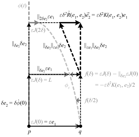
Figure 4.3: A Jacobi field is the vector field between adjacent geodesics, whose construction creates a relationship between the covariant derivative and the sectional curvature.

Then the function

$$f(t) =-\varepsilon t^{2}K(e_{1},e_{2})/2$$ (4.40)

$$=-\varepsilon t^{2}K(J,\dot{\phi})/2$$

is the difference between $J$ and its parallel transport in the direction tangent to $\phi$, i.e. it is the value of the covariant derivative along $\phi$. Since this difference is of order $t^{2}$, at $t=0$ we have

$$\mathrm{D}_{t}^{2}J=-K(J,\dot{\phi}),$$ (4.41)

or dropping the assumption that $\check{R}(e_{1},e_{2})\vec{e}_{2}$ is parallel to $e_{1}$,

$$\frac{\mathrm{D}^{2}J}{\mathrm{d}t^{2}}+\check{R}(J,\dot{\phi})\vec{\dot{\phi}}=0.$$ (4.42)

Considered as an equation for all $J(t)$, this is called the Jacobi equation, with the vector field $J(t)$ that satisfies it called a Jacobi field. A more precise way to generalize our construction of $J$ is to define a one-parameter family of geodesics $\phi_{s}(t)$, so that

$$J(t)=\left.\frac{\partial\phi_{s}(t)}{\partial s}\right|_{s=0}.$$ (4.43)

If $M$ is complete then every Jacobi field can be expressed in this way for some family of geodesics.

If we then consider the Jacobi fields $J_{v}(t)$ corresponding to the geodesics $\phi_{v}(t)$ of tangent vectors $\left\|v\right\|=1$ parametrized by arclength and such that to order $t$ we have $\left\|J_{v}(1)\right\|=1$, it can be shown ([1] pp. 114-115) that to order $t^{3}$ we have $\left\|J_{v}(t)\right\|=t(1-t^{2}K(J_{v},\dot{\phi}_{v})/6)$.

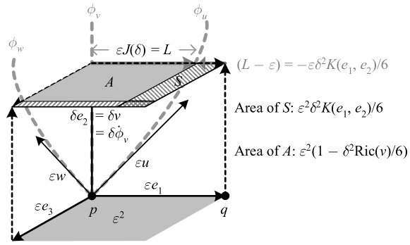
Figure 4.4: The infinitesimal geodesic area element derived from the Jacobi field between radial geodesics.

This means that if we apply the previous reasoning for parallel geodesics to these radial geodesics we have an “infinitesimal geodesic $(n-1)$-area element” $A(t)=t^{2}(1-t^{2}\mathrm{Ric}(v)/6)$. Integrating this over all values of $v$ gives for small $t=\varepsilon$ the surface area of a geodesic $n$-ball of radius $\varepsilon$, which we denote $\partial B_{\varepsilon}(M^{n})$. But this integral just averages the values of the Ricci function, which is the Ricci scalar over the dimension $n$, so that to order $\varepsilon^{2}$ we have

$$\frac{\partial B_{\varepsilon}(M^{n})}{\partial B_{\varepsilon}(\mathbb{R}^{n})}=1-\frac{\varepsilon^{2}}{6n}R,$$ (4.44)

and integrating over the radius we find (see [5]) a similar relation for the volume of a geodesic sphere compared to a Euclidean one of

$$\frac{B_{\varepsilon}(M^{n})}{B_{\varepsilon}(\mathbb{R}^{n})}=1-\frac{\varepsilon^{2}}{6(n+2)}R.$$ (4.45)

Thus $\varepsilon^{2}R/6n$ is “the fraction by which the surface area of a geodesic $n$-ball of radius $\varepsilon$ is smaller than it would be under a flat metric,” and $\varepsilon^{2}R/6(n+2)$ is “the fraction by which the volume of a geodesic $n$-ball of radius $\varepsilon$ is smaller than it would be under a flat metric.”

Alternatively, we can use Riemann normal coordinates to express $v$ in our “infinitesimal geodesic $(n-1)$-area element,” whereupon following similar logic to the above we find that, at points close to the origin of our coordinates, to order $\left\|x\right\|^{2}$ the volume element is

$$\mathrm{d}V=\left(1-\frac{1}{6}R_{\mu\nu}x^{\mu}x^{\nu}\right)\mathrm{d}x^{1}\cdots\mathrm{d}x^{n},$$ (4.46)

or using the expression of the volume element in terms the square root of the determinant of the metric, again to order $\left\|x\right\|^{2}$ we find that

$$g_{\mu\nu}=\delta_{\mu\nu}-\frac{1}{3}R_{\mu\lambda\nu\sigma}x^{\lambda}x^{\sigma}.$$ (4.47)

As is apparent from their definitions, the Ricci tensor and function do not depend on the metric. We can attempt to find a metric-free geometric interpretation by considering the concept of a parallel volume form. This is defined as a volume form which is invariant under parallel transport. We immediately see that it is only possible to define such a form if parallel transport around a loop does not alter volumes, i.e. that $\check{R}$ must be $o(r,s)$-valued. This means that the connection is metric compatible, so we can define one if we wish; but if we do not, and assume zero torsion so that the Ricci tensor is symmetric, then our logic for volumes remains valid and we can still take a metric-free view of the expression for $\mathrm{d}V$ above as expressing the geodesic volume as measured by the parallel volume form. Note that unlike the Ricci tensor and function, the definitions here of the individual sectional curvatures and scalar curvature do depend upon the metric.

4.8 Summary

Below, we review the intuitive meanings of the various relations we have defined on a Riemannian manifold.

Relation	Meaning
$\mathrm{div}(u)\mathrm{d}V=L_{u}\mathrm{d}V$	$\mathrm{div}(u)$ is the fraction by which a unit volume changes when transported by the flow of $u$.
$\begin{aligned} \int_{V}\mathrm{div}(u)\mathrm{d}V&=\int_{\partial V}i_{u}\mathrm{d}V\\ &=\int_{\partial V}\left\langle u,n\right\rangle\mathrm{d}S\end{aligned}$	The change in a volume due to transport by the flow of $u$ is equal to the net flow of $u$ across that volume’s boundary.
$\mathrm{div}(u)=0$	$u$ having zero divergence means the flow of $u$ leaves volumes unchanged, or the net flow of $u$ across the boundary of a volume is zero.
$j\equiv\rho u$, $\rho$ is the density of $Q$	The current vector $j$ is the vector whose length is the amount of $Q$ per unit time crossing a unit area perpendicular to $j$
$\begin{aligned} \frac{\mathrm{d}q}{\mathrm{d}t}&=\Sigma-\int_{\partial V}\left\langle j,n\right\rangle\mathrm{d}S\end{aligned}$	The change in $q$ (the amount of $Q$ within $V$) equals the amount generated less the amount which passes through $\partial V$.
$\begin{aligned} \frac{\partial\rho}{\partial t}&=\sigma-\mathrm{div}(j)\end{aligned}$	The change in the density of $Q$ at a point equals the amount generated less the amount that moves away.

Table 4.3: Divergence and continuity relations and their intuitive meanings.

Relation	Meaning
$R\equiv g^{ab}R_{ab}$	The Ricci scalar is $n$ times the average of the Ricci function on the set of unit tangent vectors.
$\mathrm{Ric}(e_{\mu})=\underset{i\neq\mu}{\sum}g_{\mu\mu}K(e_{i},e_{\mu})$	The Ricci function of a unit vector is $(n-1)$ times the average of the sectional curvatures of the planes that include the vector.
$R=\underset{j}{\sum}g_{jj}\mathrm{Ric}(e_{j})$	The Ricci scalar is $n$ times the average of all the Ricci functions.
$R=2\underset{i<j}{\sum}K(e_{i},e_{j})$	The Ricci scalar is $n(n-1)$ times the average of all sectional curvatures.
$\begin{aligned} G(e_{\mu},e_{\mu})&=-g_{\mu\mu}\sum_{\begin{subarray}{c}i<j\\ i,j\neq\mu\end{subarray}}K(e_{i},e_{j})\end{aligned}$	The Einstein tensor applied to a unit vector $\hat{v}$ twice is $-\left\langle\hat{v},\hat{v}\right\rangle(n-1)(n-2)/2$ times the average of the sectional curvatures of the planes orthogonal to the vector.
$\begin{aligned} d\left(\mathrm{exp}(\delta\hat{w}),\mathrm{exp}(\delta\parallel_{\varepsilon\hat{v}}\hat{w})\right)\\ =\varepsilon\left(1-\frac{\delta^{2}}{2}K(\hat{v},\hat{w})\right)\end{aligned}$	$K(\hat{v},\hat{w})/2$ is the fraction by which the geodesic parallel to $\hat{w}$ starting $\hat{v}$ away bends towards $\hat{w}$.
$\left.\frac{\ddot{L}}{L}\right|_{t=0}=-K(\hat{v},\hat{w})$	$K(\hat{v},\hat{w})$ is the acceleration of two parallel geodesics in the $\hat{w}$ direction with initial separation direction $\hat{v}$ towards each other as a fraction of the initial gap.
$\left.\frac{\ddot{A}}{A}\right|_{t=0}=-\mathrm{Ric}(v)$	$\mathrm{Ric}(v)/2$ is the fraction by which the area defined by the geodesics emanating from the $(n-1)$-surface perpendicular to $v$ changes in the direction of $v$. $\mathrm{Ric}(v)$ is the acceleration of the parallel geodesics emanating from the $(n-1)$-surface perpendicular to $v$ towards each other as a fraction of the initial surface.
$\begin{aligned} \frac{\partial B_{\varepsilon}(M^{n})}{\partial B_{\varepsilon}(\mathbb{R}^{n})}&=1-\frac{\varepsilon^{2}}{6n}R\end{aligned}$	$\varepsilon^{2}R/6n$ is the fraction by which the surface area of a geodesic $n$-ball of radius $\varepsilon$ is smaller than it would be under a flat metric.
$\begin{aligned} \frac{B_{\varepsilon}(M^{n})}{B_{\varepsilon}(\mathbb{R}^{n})}&=1-\frac{\varepsilon^{2}}{6(n+2)}R\end{aligned}$	$\varepsilon^{2}R/6(n+2)$ is the fraction by which the volume of a geodesic $n$-ball of radius $\varepsilon$ is smaller than it would be under a flat metric.

Table 4.4: Relations defined on a Riemannian manifold $M^{n}$ and their intuitive meanings.

Appendices

Appendix A Tensors and forms

It is assumed the reader is familiar with vector spaces and inner products, as well as the tensor product and the exterior product (AKA wedge product, Grassmann product). In the following, we will limit our discussion to finite-dimensional real vector spaces $V=\mathbb{R}^{n}$; generalization to complex scalars is straightforward.

A.1 The structure of the dual space

Given a finite-dimensional vector space $V$, the dual space $V^{*}$ is defined to be the set of linear mappings from $V$ to the scalars (AKA the linear functionals on $V$). The elements of $V^{*}$ can be added together and multiplied by scalars, so $V^{*}$ is also a vector space, with the same dimension as $V$.

$\triangle$ Note that in general, the word “dual” is used for many concepts in mathematics; in particular, the dual space has no relation to the Hodge dual (defined below).

An element $\varphi\colon V\to\mathbb{R}$ of $V^{*}$ is called a 1-form. Given a pseudo inner product on $V$, we can construct an isomorphism between $V$ and $V^{*}$ defined by

$$v\mapsto\left\langle v,\;\right\rangle,$$ (A.1)

i.e. $v\in V$ is mapped to the element of $V^{*}$ which maps any vector $w\in V$ to $\left\langle v,w\right\rangle$. This isomorphism then induces a corresponding pseudo inner product on $V^{*}$ defined by

$$\left\langle\left\langle v,\;\right\rangle,\left\langle w,\;\right\rangle\right\rangle\equiv\left\langle v,w\right\rangle.$$ (A.2)

An equivalent way to set up this isomorphism is to choose a basis $e_{\mu}$ of $V$, and then form the dual basis $\beta^{\nu}$ of $V^{*}$, defined to satisfy $\beta^{\lambda}(e_{\mu})=?\delta^{\lambda}{}_{\mu}?$. The isomorphism between $V$ and $V^{*}$ is then defined by the correspondence

$$v=v^{\mu}e_{\mu}\mapsto(\eta_{\mu\lambda}v^{\mu})\beta^{\lambda}\equiv v_{\lambda}\beta^{\lambda},$$ (A.3)

which is identical to the isomorphism induced by the pseudo inner product on $V$ that makes $e_{\mu}$ orthonormal. Here we have used the Einstein summation convention, i.e. a repeated index implies summation. Note that if $\left\langle e_{\mu},e_{\mu}\right\rangle=-1$ then $e_{\mu}\mapsto-\beta^{\mu}$. This isomorphism and its inverse (usually in the context of Riemannian manifolds) are called the musical isomorphisms, where if $v=v^{\mu}e_{\mu}$ and $\varphi=\varphi_{\mu}\beta^{\mu}$ we write

$$v^{\flat} \equiv\left\langle v,\;\right\rangle$$ (A.4)

$$=\left(\eta_{\mu\lambda}v^{\lambda}\right)\beta^{\mu}$$

$$=v_{\mu}\beta^{\mu}$$

$$\varphi^{\sharp} \equiv\left\langle\varphi,\;\right\rangle$$

$$=\left(\eta^{\mu\lambda}\varphi_{\lambda}\right)e_{\mu}$$

$$=\varphi^{\mu}e_{\mu}$$

and call the $v^{\flat}$ the flat of the vector $v$ and $\varphi^{\sharp}$ the sharp of the 1-form $\varphi$.

$\triangle$ It is important to remember that when the inner product is not positive definite, the signs of components may change under these isomorphisms. If the components are in terms of an arbitrary (non-orthonormal) basis, then as we will see in Section A.4, the components change their values as well, since $\eta_{\lambda\mu}$ is replaced by the metric tensor in the above analysis.

Note that since $\beta^{\lambda}(e_{\mu})=?\delta^{\lambda}{}_{\mu}?$ and $\left\langle e_{\mu},e_{\lambda}\right\rangle=\eta_{\mu\lambda}$ we have

$$\varphi(v) =\varphi_{\lambda}\beta^{\lambda}(v^{\mu}e_{\mu})$$ (A.5)

$$=\varphi_{\mu}v^{\mu}$$

$$=\eta_{\mu\lambda}\varphi^{\lambda}v^{\mu}$$

$$=\left\langle\varphi^{\sharp},v\right\rangle.$$

A 1-form acting on a vector can thus be viewed as yielding a projection. Specifically, with a positive definite inner product, $\varphi(v)/\left\|\varphi^{\sharp}\right\|$ is the length of the projection of $v$ onto the ray defined by $\varphi^{\sharp}$. If we then define

$$\varphi^{\Uparrow}\equiv\varphi^{\sharp}/\left\|\varphi^{\sharp}\right\|^{2},$$ (A.6)

the length of this projection as a multiple of $\left\|\varphi^{\Uparrow}\right\|$ is

$$\left\langle\varphi^{\Uparrow},v\right\rangle/\left\|\varphi^{\Uparrow}\right\|=\varphi(v).$$ (A.7)

We can therefore represent a 1-form $\varphi$ as a “receptacle” $\varphi^{\Uparrow}$ which when applied to a vector “arrow” argument $v$ yields the number of receptacles covered by the projection of $v$ onto $\varphi^{\sharp}$, which is the value of $\varphi(v)$. The advantage of this approach is that values can be calculated from a figure absent a length scale. Another common graphical device is to represent $\varphi$ as a density of “surfaces” where the value of $\varphi(v)$ is the number of surfaces “pierced” by the arrow. Figure A.1 covers some non-intuitive aspects of these visualizations.

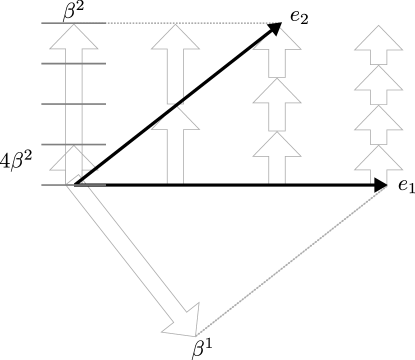
Figure A.1: Depicting a 1-form $\varphi$ as the associated vector $\varphi^{\Uparrow}$ or as a density of surfaces has consequences that can be non-intuitive. When orthogonality corresponds to right angles in a figure, an orthonormal basis and its dual basis appear as identical arrows; in the figure, we see that for a non-orthonormal basis, the dual basis does not appear to either be parallel to the basis or to have identical lengths. We also see that quadrupling the value of the 1-form means quartering its length in the figure, or equivalently quadrupling the density of surfaces pierced by arrows. This means that when depicting a linearly changing 1-form as above, the length $L$ of the associated vector changes like $L\mapsto L/(1+r\varepsilon)$ for some scaling factor $r$, which doesn’t appear linear as a vector representation would, whose length changes like $L\mapsto L(1+r\varepsilon)$.

$\triangle$ It is important to remember that the practice of depicting a 1-form $\varphi$ as the associated vector $\varphi^{\Uparrow}$ or as a density of surfaces has consequences that can be non-intuitive.

It is important to note that there is no canonical isomorphism between $V$ and $V^{*}$, i.e. we cannot uniquely associate a 1-form with a given vector without introducing extra structure, namely an inner product or a preferred basis. Either structure will do: a choice of basis is equivalent to the definition of the unique inner product on $V$ that makes this basis orthonormal, which then induces the same isomorphism as that induced by the dual basis.

In contrast, a canonical isomorphism $V\cong V^{**}$ can be made via the association $v\in V\leftrightarrow\xi\in V^{**}$ with $\mathbb{\xi}\colon V^{*}\to\mathbb{R}$ defined by $\xi\left(\varphi\right)\equiv\varphi\left(v\right)$. Thus $V$ and $V^{**}$ can be completely identified (for a finite-dimensional vector space), and we can view $V$ as the dual of $V^{*}$, with vectors regarded as linear mappings on 1-forms.

Vector components are often viewed as a column vector, which means that 1-forms act on vector components as row vectors (which then are acted on by matrices from the right). Under a change of basis we then have the following relationships:

	Index notation	Matrix notation
Basis	$e_{\mu}^{\prime}=A^{\lambda}{}_{\mu}e_{\lambda}$	$e^{\prime}=eA$
Dual basis	$\beta^{\prime\mu}=(A^{-1})^{\mu}{}_{\lambda}\beta^{\lambda}$	$\beta^{\prime}=A^{-1}\beta$
Vector components	$\left(v^{\mu}\right)^{\prime}=(A^{-1})^{\mu}{}_{\lambda}v^{\lambda}$	$v^{\prime}=A^{-1}v$
1-form components	$\left(\varphi_{\mu}\right)^{\prime}=A^{\lambda}{}_{\mu}\varphi_{\lambda}$	$\varphi^{\prime}=\varphi A$

Table A.1: Transformations under a change of basis.

Notes: We notationally distinguish between a changed vector $e_{\mu}^{\prime}$ and an unchanged vector with changed components $\left(v^{\mu}\right)^{\prime}$. A 1-form will sometimes be viewed as a column vector, i.e. as the transpose of the row vector (which is the sharp of the 1-form under a Riemannian signature). Then we have $(\varphi^{\prime})^{T}=(\varphi A)^{T}=A^{T}\varphi^{T}$.

A.2 Tensors

A tensor of type (AKA valence) $\left(m,n\right)$ is defined to be an element of the tensor space

$$V_{m,n}\equiv\left(V\otimes\dotsb\left(m\>\textrm{times}\right)\dotsb\otimes V\right)\otimes\left(V^{*}\otimes\dotsb\left(n\>\textrm{times}\right)\dotsb\otimes V^{*}\right).$$ (A.8)

A pure tensor (AKA simple or decomposable tensor) of type $\left(m,n\right)$ is one that can be written as the tensor product of $m$ vectors and $n$ 1-forms; thus a general tensor is a sum of pure tensors. The integer $\left(m+n\right)$ is called the order (AKA degree, rank) of the tensor, while the tensor dimension is that of $V$. Vectors and 1-forms are then tensors of type $\left(1,0\right)$ and $\left(0,1\right)$. The rank (sometimes used to refer to the order) of a tensor is the minimum number of pure tensors required to express it as a sum. In “tensor language” vectors $v\in V$ are called contravariant vectors and 1-forms $\varphi\in V^{*}$ are called covariant vectors (AKA covectors). A tensor of type $\left(k,0\right)$ is then called a contravariant tensor, with covariant tensors being of type $\left(0,k\right)$, and other tensor types being called mixed tensors. Scalars can be considered tensors of type $\left(0,0\right)$.

$\triangle$ As noted above, the meanings of tensor rank and order are often swapped in the literature. Another potential source of confusion is that a mixed tensor is not the opposite of a pure tensor.

The infinite direct sum of the tensor spaces of every type forms an associative algebra. This algebra is also called the “tensor algebra,” and “tensor” sometimes refers to the general elements of this algebra, in which case tensors as defined above are called homogeneous tensors. In this book, we will always use the term “tensor” to mean homogeneous tensor, while for “tensor algebra” the inclusion of powers of the dual space will depend upon context.

A.3 Tensors as multilinear mappings

There is an obvious multiplication of two 1-forms: the scalar multiplication of their values. The resulting object $\varphi\psi\colon V\times V\to\mathbb{R}$ is a nondegenerate bilinear form on $V$. Viewed as an “outer product” on $V^{*}$, multiplication is trivially seen to be a bilinear operation, i.e. $a\left(\varphi+\psi\right)\xi=a\varphi\xi+a\psi\xi$. Thus the product of two 1-forms is isomorphic to their tensor product.

We can extend this to any tensor by viewing vectors as linear mappings on 1-forms, and forming the isomorphism

$$\bigotimes\varphi_{i}\mapsto\prod\varphi_{i}.$$ (A.9)

Note that this isomorphism is not unique, since for example any real multiple of the product would yield a multilinear form as well. However it is canonical, since the choice does not impose any additional structure, and is also consistent with considering scalars as tensors of type $\left(0,0\right)$.

We can thus consider tensors to be multilinear mappings on $V^{*}$ and $V$. In fact, we can view a tensor of type $\left(m,n\right)$ as a mapping from $i<m$ 1-forms and $j<n$ vectors to the remaining $\left(m-i\right)$ vectors and $\left(n-j\right)$ 1-forms.

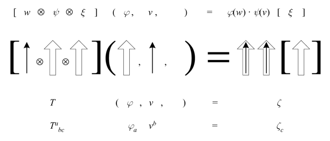
Figure A.2: Different ways of depicting a pure tensor of type $\left(1,2\right)$. The first line explicitly shows the tensor as a mapping from a 1-form $\varphi$ and a vector $v$ to a 1-form $\xi$. The second line visualizes vectors as arrows, and 1-forms as receptacles that when matched to an arrow yield a scalar. The third line combines the constituent vectors and 1-forms of the tensor into a single symbol $T$ while merging the scalars into $\xi$ to define $\zeta$, and the last line adds indices (covered in the next section).

A general tensor is a sum of pure tensors, so for example a tensor of the form $\left(u\otimes\varphi\right)+\left(v\otimes\psi\right)$ can be viewed as a linear mapping that takes $\xi$ and $w$ to the scalar $\xi\left(u\right)\cdot\varphi\left(w\right)+\xi\left(v\right)\cdot\psi\left(w\right)$. Since the roles of mappings and arguments can be reversed, we can simplify things further by viewing the arguments of a tensor as another tensor:

$$\left(u\otimes\varphi\right)\left(\xi\otimes w\right) \equiv\left(u\otimes\varphi\right)\left(\xi,w\right)$$ (A.10)

$$=\left(\xi\otimes w\right)\left(u,\varphi\right)$$

$$=\xi\left(u\right)\cdot\varphi\left(w\right)$$

A.4 Abstract index notation

Abstract index notation uses an upper Latin index to represent each contravariant vector component of a tensor, and a lower index to represent each covariant vector (1-form) component. We can see from the preceding figure that this notation is quite compact and clearly indicates the type of each tensor while re-using letters to indicate what “slots” are to be used in the mapping.

The tensor product of two tensors $?S^{a}{}_{b}?\otimes?T^{c}{}_{d}?$ is simply denoted $?S^{a}{}_{b}??T^{c}{}_{d}?$, and in this form the operation is sometimes called the tensor direct product. We may also consider a contraction

$$?T^{ab}{}_{bc}?=?T^{a}{}_{c}?,$$ (A.11)

where two of the components of a tensor operate on each other to create a new tensor with a reduced number of indices. For example, if $?T^{ab}{}_{c}?=v^{a}\otimes w^{b}\otimes\varphi_{c}$, then $?T^{ab}{}_{b}?=\varphi(w)\cdot v^{a}$. Taking the tensor direct product of two tensors and then contracting all opposite indices is also called the contraction of the two tensors, i.e. the contraction of $?S^{ab}{}_{c}?$ and $?T_{def}?$ is $?C_{cf}?=?S^{ab}{}_{c}??T{}_{abf}?$. The contraction of any two symmetric indices with any two anti-symmetric indices vanishes, e.g. if the (first) second tensor is (anti) symmetric in the first two indices then

$$S^{abc}T_{abd}=-S^{bac}T_{bad}=-S^{abc}T_{abd},$$ (A.12)

where in the last step we relabel “dummy” indices summed over. Similarly, any tensor with overlapping anti-symmetric and symmetric indices vanishes, e.g. if the (first) second two indices are (anti) symmetric then

$$T^{abc}=-T^{bac}=-T^{bca}=T^{cba}=T^{cab}=-T^{acb}=-T^{abc}.$$ (A.13)

A (pseudo) inner product on $V$ is a symmetric bilinear mapping, and thus corresponds to a symmetric tensor $g_{ab}$ called the (pseudo) metric tensor. The isomorphism $v\in V\mapsto v^{\flat}\in V^{*}$ induced by this pseudo inner product is then defined by

$$v^{a}\mapsto v_{a}\equiv g_{ab}v^{b},$$ (A.14)

and is called index lowering. The dual metric tensor (AKA conjugate metric tensor) is the corresponding pseudo inner product on $V^{*}$ and is denoted $g^{ab}$, which provides a consistent index raising operation since we immediately obtain $g^{ab}g_{ac}g_{bd}=g_{cd}$. We also have the relation $v^{a}=g^{ab}v_{b}=g^{ab}g_{bc}v^{c}\Rightarrow g^{ab}g_{bc}=?g^{a}{}_{c}?=?\delta^{a}{}_{c}?$, the identity mapping; thus $g^{ab}g_{ab}$ is equal to the dimension of $V$. The inner product of two tensors of the same type is then the contraction of their tensor direct product after index lowering/raising, e.g. $\left\langle T^{ab},S^{cd}\right\rangle=T^{ab}S_{ab}=T^{ab}g_{ac}g_{bd}S^{cd}$.

$\triangle$ It is important to remember that if $v$ is a vector, the operation $v_{a}v^{a}$ implies index lowering, which requires an inner product. In contrast, if $\varphi$ is a 1-form, the operation $\varphi_{a}v^{a}$ is always valid regardless of the presence of an inner product.

A symmetric or anti-symmetric tensor can be formed from a general tensor by adding or subtracting versions with permuted indices. For example, the combination $\left(T_{ab}+T_{ba}\right)/2$ is the symmetrized tensor of $T$, i.e. exchanging any two indices leaves it invariant. The anti-symmetrized tensor $\left(T_{ab}-T_{ba}\right)/2$ changes sign upon the exchange of any two indices, and (only for tensors of order 2) yields the original tensor $T_{ab}$ when added to the symmetrized tensor. The following notation is common for tensors with $n$ indices, with the sums over all permutations of indices:

$$\textrm{Symmetrization:}\;T_{\left(a_{1}\dots a_{n}\right)}\equiv\frac{1}{n!}\underset{\pi}{\sum}T_{a_{\pi\left(1\right)}\dots a_{\pi\left(n\right)}}$$ (A.15)

$$\textrm{Anti-symmetrization:}\;T_{\left[a_{1}\dots a_{n}\right]}\equiv\frac{1}{n!}\underset{\pi}{\sum}\textrm{sign}\left(\pi\right)T_{a_{\pi\left(1\right)}\dots a_{\pi\left(n\right)}}$$ (A.16)

This operation can be performed on any subset of indices in a tensor, as long as they are all covariant or all contravariant. Skipping indices is denoted with vertical bars, as in $T_{\left(a|b|c\right)}=\left(T_{abc}+T_{cba}\right)/2$; however, note that vertical bars alone are sometimes used to denote a sum of ordered permutations, as in $T_{\left|abc\right|}=T_{abc}+T_{bca}+T_{cab}$.

A.5 Tensors as multi-dimensional arrays

In a given basis, a pure tensor of type $(m,n)$ can be written using component notation in the form

$$v^{1}\otimes\dotsb\otimes v^{m}\otimes\varphi_{1}\otimes\dotsb\otimes\varphi_{n}\equiv?T^{\mu_{1}\dots\mu_{m}}{}_{\lambda_{1}\dots\lambda_{n}}?e_{\mu_{1}}\otimes\dotsb\otimes e_{\mu_{m}}\otimes\beta^{\lambda_{1}}\otimes\dotsb\otimes\beta^{\lambda_{n}},$$ (A.17)

where the Einstein summation convention is used in the second expression. Note that the collection of terms into $T$ is only possible due to the defining property of the tensor product being linear over addition. The tensor product between basis elements is often dropped in such expressions. Also note that this means that in terms of the tensor as a multilinear mapping we have

$$?T^{\mu_{1}\dots\mu_{m}}{}_{\lambda_{1}\dots\lambda_{n}}?=T\left(\beta^{\mu_{1}},\dotsb,\beta^{\mu_{m}},e_{\lambda_{1}},\dotsb,e_{\lambda_{n}}\right).$$ (A.18)

A general tensor is a sum of such pure tensor terms, so that any tensor $T$ can be represented by a $\left(m+n\right)$-dimensional array of scalars. For example, any tensor of order 2 is a matrix, and type $(1,1)$ tensors are linear mappings operating on vectors or forms via ordinary matrix multiplication if they are all expressed in terms of components in the same basis. Basis-independent quantities from linear algebra such as the trace and determinant are then well defined on such tensors.

$\triangle$ It is important to remember that a tensor $T^{\mu\nu}$ or $T_{\mu\nu}$ can be written as a matrix of scalars, but linear algebra operations only are valid for linear operators $?T^{\mu}{}_{\nu}?$. A similar source of potential confusion is that the (anti-)symmetry of $T^{\mu\nu}$ or $T_{\mu\nu}$ is basis independent, while that of $?T^{\mu}{}_{\nu}?$ is not.

$\triangle$ A potentially confusing aspect of component notation is the basis vectors $e_{\mu}$, which are not components of a 1-form but rather vectors, with $\mu$ a label, not an index. Similarly, the basis 1-forms $\beta^{\lambda}$ should not be confused with components of a vector.

The Latin letters of abstract index notation (e.g. $?T^{ab}{}_{cd}?$) can thus be viewed as placeholders for what would be indices in a particular basis, while the Greek letters of component notation represent an actual array of scalars that depend on a specific basis. The reason for the different notations is to clearly distinguish tensor identities, true in any basis, from equations true only in a specific basis.

$\triangle$ It is common in general relativity and other topics to abuse both abstract and index notation to represent objects that are non-tensorial (see Section 2).

$\triangle$ Note that if abstract index notation is not being used, Latin and Greek indices are often used to make other distinctions, a common one being between indices ranging over three space indices and indices ranging over four space-time indices.

$\triangle$ Note that “rank” and “dimension” are overloaded terms across these constructs: “rank” is sometimes used to refer to the order of the tensor, which is the dimensionality of the corresponding multi-dimensional array; the dimension of a tensor is that of the underlying vector space, and so is the length of a side of the corresponding array (also sometimes called the dimension of the array). However, the rank of a order 2 tensor coincides with the rank of the corresponding matrix.

A.6 Exterior forms as multilinear mappings

An exterior form (AKA $k$-form, alternating form) is defined to be an element of $\Lambda^{k}V^{*}$. Just as we formed the isomorphism $\otimes\varphi_{i}\mapsto\Pi\varphi_{i}$ to view tensors as multilinear mappings on $V$, we can view $k$-forms as alternating multilinear mappings on $V$. Restricting attention to the exterior product of $k$ 1-forms $\bigwedge\varphi_{i}$, we define the isomorphism

$$\bigwedge_{i=1}^{k}\varphi_{i} \mapsto\sum_{\pi}\textrm{sign}\left(\pi\right)\prod_{i=1}^{k}\varphi_{\pi\left(i\right)}$$ (A.19)

$$=\sum_{i_{1},i_{2},\dotsc,i_{k}}\varepsilon^{i_{1}i_{2}\dots i_{k}}\varphi_{i_{1}}\varphi_{i_{2}}\dotsm\varphi_{i_{k}},$$

where $\pi$ is any permutation of the $k$ indices, sign$(\pi)$ is the sign of the permutation, and $\varepsilon$ is the permutation symbol (AKA completely anti-symmetric symbol, Levi-Civita symbol, alternating symbol, $\varepsilon$-symbol), defined to be $+1$ for even index permutations, $-1$ for odd, and $0$ otherwise.

☼ The above isomorphism extends the interpretation of forms acting on vectors as yielding a projection. Specifically, if the parallelepiped $\varphi^{\sharp}=\bigwedge\varphi_{i}^{\sharp}$ has volume $V$, then $\varphi(v_{1},\ldots v_{k})/V$ is the volume of the projection of the parallelepiped $v=\bigwedge v_{i}$ onto $\varphi^{\sharp}$.

Extending this to arbitrary forms $\varphi\in\Lambda^{j}V^{*}$ and $\psi\in\Lambda^{k}V^{*}$, we have

$$\left(\varphi\wedge\psi\right)\left(v_{1},\dotsc,v_{j+k}\right)$$ (A.20)

$$\mapsto\cfrac{1}{j!k!}\sum_{\pi}\textrm{sign}\left(\pi\right)\varphi\left(v_{\pi\left(1\right)},\dotsc,v_{\pi\left(j\right)}\right)\psi\left(v_{\pi\left(j+1\right)},\dotsc,v_{\pi\left(j+k\right)}\right).$$

Just as with tensors, this isomorphism is canonical but not unique; but in the case of exterior forms, other isomorphisms are in common use. The main alternative isomorphism inserts a term $1/k!$ in the first relation above, which results in $1/j!k!$ being replaced by $1/\left(j+k\right)!$ in the second. Note that this alternative is inconsistent with the interpretation of exterior products as parallelepipeds.

$\triangle$ It is important to understand which convention a given author is using. The first convention above is common in physics, and we will adhere to it here.

A.7 Exterior forms as completely anti-symmetric tensors

An immediate result of this view of forms as multilinear mappings is that we can also view forms as completely anti-symmetric tensors under the identification of $\prod\varphi_{i}$ with $\bigotimes\varphi_{i}$. For example, for a 2-form we have the equivalent expressions

$$\left(\varphi\wedge\psi\right)\left(v,w\right) \leftrightarrow\left(\varphi\otimes\psi-\psi\otimes\varphi\right)\left(v,w\right)$$ (A.21)

$$\leftrightarrow\varphi\left(v\right)\psi\left(w\right)-\psi\left(v\right)\varphi\left(w\right).$$

Note however that this identification does not lead to equality of the inner products defined on tensors and exterior forms; instead for two $k$-forms we have

$$\left\langle\bigwedge\varphi_{i},\bigwedge\psi_{j}\right\rangle_{\textrm{form}}=\textrm{det}\left(\left\langle\varphi_{i},\psi_{j}\right\rangle\right),$$ (A.22)

while as tensors we have

$$\left\langle\bigwedge\varphi_{i},\bigwedge\psi_{j}\right\rangle_{\textrm{tensor}}=\left\langle\varepsilon^{I}\varphi_{I},\varepsilon^{J}\varphi_{J}\right\rangle_{\textrm{tensor}}=k!\textrm{det}\left(\left\langle\varphi_{i},\psi_{j}\right\rangle\right).$$ (A.23)

Fortunately, the tensor inner product is almost always expressed explicitly in terms of index contractions, so we will continue to use the $\left\langle\;,\,\right\rangle$ notation for the inner product of $k$-forms.

Also note that this isomorphism between the exterior product and the tensor product can be similarly used to identify the exterior product of vectors with a completely anti-symmetric contravariant tensor. In the following section we identify exterior forms with lower index anti-symmetric arrays; we can similarly identify the exterior product of vectors with upper index anti-symmetric arrays.

A.8 Exterior forms as anti-symmetric arrays

In terms of a basis $\beta^{\mu}$ of $V^{*}$, we can write a $k$-form $\varphi$ as

$$\varphi=\frac{1}{k!}\sum_{\mu_{1},\dotsc,\mu_{k}}\varphi_{\mu_{1}\dots\mu_{k}}\beta^{\mu_{1}}\wedge\dotsb\wedge\beta^{\mu_{k}}.$$ (A.24)

$\triangle$ The above way of writing the components is not unique, and others are in common use, the main alternative omitting the factorial.

The advantage of the expression above is that, with our isomorphism convention, the component array can be identified with the anti-symmetric covariant tensor component array in the same basis:

$$\varphi\mapsto\frac{1}{k!}\varphi_{\mu_{1}\dots\mu_{k}}\sum_{\pi}\textrm{sign}\left(\pi\right)\bigotimes_{i}\beta^{\pi\left(i\right)}=\varphi_{\mu_{1}\dots\mu_{k}}\beta^{\mu_{1}}\otimes\cdots\otimes\beta^{\mu_{k}}$$ (A.25)

Here we have dropped the summation sign in favor of the Einstein summation convention, and the last equality follows from the anti-symmetry of the component array. This means that as with tensors, in terms of the $k$-form as a multilinear mapping we have

$$\varphi_{\mu_{1}\dots\mu_{k}}=\varphi\left(e_{\mu_{1}},\dotsb,e_{\mu_{k}}\right).$$ (A.26)

A.9 Algebra-valued exterior forms

We can extend the view of exterior forms as real-valued linear mappings to define algebra-valued forms. These follow the same construction as in Section A.6 above, starting from an algebra-valued 1-form

$$\check{\Theta}\colon V\to\mathfrak{a},$$ (A.27)

so that general forms are alternating multilinear maps from $k$ vectors to a real algebra $\mathfrak{a}$ whose vector multiplication takes the place of multiplication in $\mathbb{R}$. Since this vector multiplication may not be commutative, we need to be more careful in terms of ordering in the isomorphism to ensure antisymmetry, i.e. for two algebra-valued 1-forms we define

$$(\check{\Theta}\wedge\check{\Psi})(v,w)\equiv\check{\Theta}(v)\check{\Psi}(w)-\check{\Theta}(w)\check{\Psi}(v).$$ (A.28)

An algebra-valued form whose values are defined by matrices is a matrix-valued form. Exterior forms that take values in a matrix group can also be considered as matrix-valued forms, but it must be understood that under addition the values may no longer be in the group. One can also form the exterior product between a matrix-valued form and a vector-valued form. To reduce confusion when dealing with algebra- and vector-valued forms, we will indicate them with (non-standard) decorations, for example in the case of a matrix-valued 1-form acting on a vector-valued 1-form,

$$(\check{\Theta}\wedge\vec{\varphi})(v,w)\equiv\check{\Theta}(v)\vec{\varphi}(w)-\check{\Theta}(w)\vec{\varphi}(v).$$ (A.29)

$\triangle$ Since the elements of an algebra are vectors, algebra-valued forms may be considered as vector-valued forms whose values can be multiplied. We will reserve the term vector-valued forms for forms whose values are acted on by matrix-valued forms.

$\triangle$ An additional distinction can be made between forms that take values which are concrete matrices and column vectors (and thus depend upon the basis of the underlying vector space), and forms that take values which are abstract linear transformations and abstract vectors (and thus are basis-independent). We will attempt to distinguish between these by referring to the specific matrix or abstract group, and by only using “vector-valued” when the value is an abstract vector.

A notational issue arises in the particular case of Lie algebra valued forms, where the related associative algebra in the relation $[\check{\Theta},\check{\Psi}]=\check{\Theta}\check{\Psi}-\check{\Psi}\check{\Theta}$ could also be in use. In this case multiplication of values could use either the Lie commutator or that of the related associative algebra. We will denote the exterior product using the Lie commutator by $\check{\Theta}[\wedge]\check{\Psi}$. Some authors use $[\check{\Theta},\check{\Psi}]$ or $[\check{\Theta}\wedge\check{\Psi}]$, but both can be ambiguous, motivating us to introduce our (non-standard) notation. The expression $\check{\Theta}\wedge\check{\Psi}$ is then reserved for the exterior product using the underlying associative algebra (e.g. that of matrix multiplication if the associative algebra is defined this way). For two Lie algebra-valued 1-forms we then have

$$(\check{\Theta}[\wedge]\check{\Psi})\left(v,w\right) =[\check{\Theta}\left(v\right),\check{\Psi}\left(w\right)]-[\check{\Theta}\left(w\right),\check{\Psi}\left(v\right)]$$ (A.30)

$$=\check{\Theta}\left(v\right)\check{\Psi}\left(w\right)-\check{\Psi}\left(w\right)\check{\Theta}\left(v\right)-\check{\Theta}\left(w\right)\check{\Psi}\left(v\right)+\check{\Psi}\left(v\right)\check{\Theta}\left(w\right)$$

$$=(\check{\Theta}\wedge\check{\Psi}+\check{\Psi}\wedge\check{\Theta})\left(v,w\right).$$

Note that $[\check{\Theta},\check{\Psi}](v,w)=\check{\Theta}(v)\check{\Psi}(w)-\check{\Psi}(v)\check{\Theta}(w)$ is a distinct construction, as is $[\check{\Theta}(v),\check{\Psi}(w)]=\check{\Theta}(v)\check{\Psi}(w)-\check{\Psi}(w)\check{\Theta}(v)$; neither are in general anti-symmetric and thus do not yield forms. Also note that e.g. for two 1-forms $\check{\Theta}[\wedge]\check{\Psi}\neq\check{\Theta}\wedge\check{\Psi}-\check{\Psi}\wedge\check{\Theta}$, and $(\check{\Theta}[\wedge]\check{\Theta})\left(v,w\right)=2[\check{\Theta}\left(v\right),\check{\Theta}\left(w\right)]$ does not in general vanish, so $[\wedge]$ does not act like a Lie commutator in these respects. However, for algebra-valued $j$- and $k$-forms $\check{\Theta}$ and $\check{\Psi}$, the operation $[\wedge]$ does in fact follow a graded commutativity rule

$$\check{\Theta}[\wedge]\check{\Psi}=\left(-1\right)^{jk+1}\check{\Psi}[\wedge]\check{\Theta},$$ (A.31)

and with an algebra-valued $m$-form $\check{\Xi}$ we find a graded Jacobi identity of

$$\left(-1\right)^{jm}(\check{\Theta}[\wedge]\check{\Psi})\left[\wedge\right]\check{\Xi}+\left(-1\right)^{kj}(\check{\Psi}[\wedge]\check{\Xi})\left[\wedge\right]\check{\Theta}+\left(-1\right)^{mk}(\check{\Xi}[\wedge]\check{\Theta})\left[\wedge\right]\check{\Psi}=0.$$ (A.32)

Algebra-valued forms also introduce potentially ambiguous index notation. If a basis is chosen for the algebra $\mathfrak{a}$, the value of an algebra-valued form may be expressed using component notation as $\Theta^{\mu}$; or if the algebra is defined in terms of matrices, an element might be written $?\Theta^{\alpha}{}_{\beta}?$, an expression that has nothing to do with the basis of $\mathfrak{a}$. Then for example an algebra-valued 1-form might be written $?\Theta^{\mu}{}_{\gamma}?$ or $?\Theta^{\alpha}{}_{\beta\gamma}?$.

$\triangle$ In considering algebra-valued forms expressed in index notation, extra care must be taken to identify the type of form in question, and to match each index with the aspect of the object it was meant to represent.

A.10 The Hodge star

A pseudo inner product determines orthonormal bases for $V$, among which we can choose a specific one $\hat{e}_{\mu}$. The ordering of the $\hat{e}_{\mu}$ determines a choice of orientation. This orientation uniquely determines an orthonormal basis (i.e. a unit “length” vector) for the one-dimensional vector space $\Lambda^{n}V$, namely the unit $n$-vector (AKA orientation $n$-vector, volume element)

$$\Omega\equiv\hat{e}_{1}\wedge\dotsb\wedge\hat{e}_{n}.$$ (A.33)

$\triangle$ Many symbols are used in the literature for the unit $n$-vector and related quantities, including $\varepsilon$, $i$, $I$, and $\omega$; to avoid confusion with the other common uses of these symbols, we will use the (non-standard) symbol $\Omega$.

Since $\Lambda^{n}V$ is one-dimensional, every element of $\Lambda^{n}V$ is a real multiple of $\Omega$. Thus $\Omega$ sets up a bijection (dependent upon the inner product and choice of orientation) between $\Lambda^{n}V$ and $\Lambda^{0}V$ = $\mathbb{R}$. In general, $\Lambda^{k}V$ and $\Lambda^{n-k}V$ are vector spaces of equal dimension, and thus we can also set up a bijection between them.

The Hodge star operator (AKA Hodge dual) is defined to be the linear map

$$*\colon\Lambda^{k}V\to\Lambda^{n-k}V$$ (A.34)

that acts on any $A,B\in\Lambda^{k}V$ such that

$$A\wedge*B=\left\langle A,B\right\rangle\Omega.$$ (A.35)

In particular, we immediately obtain

$$A\wedge*A=\left\langle A,A\right\rangle\Omega.$$ (A.36)

☼ These relations allow one to think of the Hodge star $*$ as an operator that that yields the “orthogonal complement with the same magnitude,” or alternatively that “swaps the exterior and inner products.”

The Hodge star operator is dependent upon a choice of inner product and orientation, but beyond that is independent of any particular basis. However, if we choose an orthonormal basis $\hat{e}_{\mu}$ oriented with $\Omega$, we can take $\hat{A}\equiv\hat{e}_{1}\wedge\dotsb\wedge\hat{e}_{k}$ and $\hat{C}\equiv\hat{e}_{k+1}\wedge\dotsb\wedge\hat{e}_{n}$, in which case $*\hat{A}=\left\langle\hat{A},\hat{A}\right\rangle\hat{C}$, i.e. $*\hat{A}$ is constructed from an orthonormal basis for the orthogonal complement of $\hat{A}$; in fact, this relation can be used as an equivalent definition of the Hodge star, and for a pseudo inner product of signature $(r,s)$ results in

$$\left\langle A,B\right\rangle=(-1)^{s}\left\langle*A,*B\right\rangle.$$ (A.37)

Below we list some easily derived facts about the Hodge star operator, where $V$ is $n$-dimensional with unit $n$-vector $\Omega$ and a pseudo inner product of signature $(r,s)$:

• $*\Omega=\left(-1\right)^{s}\Rightarrow\left(*C\right)\Omega=\left(-1\right)^{s}C$ if $C\in\Lambda^{n}V$

• $*1=\Omega\Rightarrow\left\langle*a,\Omega\right\rangle=\left(-1\right)^{s}a$ if $a\in\Lambda^{0}V$

• $**A=\left(-1\right)^{k\left(n-k\right)+s}A=\left(-1\right)^{k\left(n-1\right)+s}A$, where $A\in\Lambda^{k}V$

• $A\wedge*B=B\wedge*A$ if $A,B\in\Lambda^{k}V$

• $*\left(A\wedge*B\right)=\left\langle A\wedge*B,\Omega\right\rangle=(-1)^{s}\left\langle A,B\right\rangle$ if $A,B\in\Lambda^{k}V$

$\triangle$ Some texts (including earlier versions of this paper and the first edition of the book based upon it) instead define the Hodge star by the relation $A\wedge C=\left\langle*A,C\right\rangle\Omega$ for $A\in\Lambda^{k}V$, $C\in\Lambda^{n-k}V$, which prefixes our current Hodge star by the factor $(-1)^{s}$.

Note that $*A$ is not a basis-independent object, since it reverses sign upon changing the chosen orientation. Such an object is prefixed by the word pseudo-, e.g. $*v$ is called a pseudo-vector (AKA axial vector, in which case $v$ is called a polar vector) and $\Omega$ itself is a pseudo-scalar.

$\triangle$ The use of “pseudo” to indicate a quantity that reverses sign upon a change of orientation should not be confused with the use of “pseudo” to indicate an inner product that is not positive-definite. There are also other uses of “pseudo” in use. In particular, in general relativity the term “pseudo-tensor” is sometimes used, where neither of the above meanings are implied; instead this signifies that the tensor (to be defined in A.2) is not in fact a tensor.

Appendix B Differentiable manifolds

Differentiable manifolds allow us to graft calculus onto a topological manifold, which we can think of as a “rubber sheet.” The constructions of coordinates and tangent vectors enable us to define a family of derivatives associated with the concept of how vector fields change on the manifold. The challenge is in defining all these objects without an ambient space, which our intuitive picture normally depends upon.

$\triangle$ Note that a differentiable manifold includes no concept of length or distance (a metric), and no structure that allows tangent vectors at different points to be compared or related to each other (a connection). It is important to remember that nothing in this section depends upon these two extra structures.

When dealing with manifolds, there are two main approaches one can take: express everything in terms of coordinates, or strive to express everything in a coordinate-free fashion. In keeping with our attempt to focus on concepts rather than calculations, we will take the latter approach, but will take pains to carefully express fundamental concepts in terms of coordinates in order to derive a picture of what these coordinate-free tools do.

B.1 Coordinates

A key feature of a topological manifold $M^{n}$ is that every point has an open neighborhood homeomorphic to an open subset of $\mathbb{R}^{n}$. To make this precise we define the following terms.

• Coordinate chart (AKA parameterization, patch, system of coordinates): a homeomorphism $\alpha\colon U\to\mathbb{R}^{n}$ from an open set $U\subset M^{n}$ to an open subset of $\mathbb{R}^{n}$

• Coordinate functions (AKA coordinates): the maps $a^{\mu}\colon U\to\mathbb{R}$ that project $\alpha$ down to one of the canonical Cartesian components

• Atlas: a collection of coordinate charts that cover the manifold

• Coordinate transformation (AKA change of coordinates, transition function): in a region covered by two charts, we can construct the map $\alpha_{2}\circ\alpha_{1}^{-1}\colon\mathbb{R}^{n}\to\mathbb{R}^{n}$

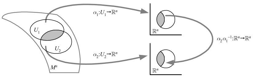
Figure B.1: In the intersection of two coordinate charts we can construct the coordinate transformation, a homeomorphism on $\mathbb{R}^{n}$.

$\triangle$ A coordinate chart is sometimes defined to be the inverse map $\alpha^{-1}\colon\mathbb{R}^{n}\to M$ valid on an open subset of $\mathbb{R}^{n}$, with similar changes to related definitions such as coordinate functions.

The coordinate transformations are simply maps on Euclidean space, so we can require them to be infinitely differentiable (AKA smooth, $C^{\infty}$). An atlas whose charts all have smooth coordinate transformations determines a differentiable structure, which turns the topological manifold into a differentiable manifold (AKA smooth manifold). Two differential structures are considered to be equivalent if the union of their atlases still results in smooth coordinate transformations. Unless otherwise noted, from this point forward “manifold” will mean differentiable manifold.

A complex manifold is defined to have an atlas of charts to $\mathbb{C}^{n}$ whose coordinate transformations are analytic. Complex $n$-manifolds are a subset of real $2n$-manifolds, but atlases are highly constrained since complex analytic functions are much more constrained than smooth functions. By “manifold” we will always mean a real manifold.

With the addition of a differentiable structure, one can define the various tools of calculus on manifolds in a straightforward way. Differentiable functions $f\colon U\to\mathbb{R}$ require the map $f\circ\alpha^{-1}\colon\mathbb{R}^{n}\to\mathbb{R}$ to be differentiable, and differentials $\partial/\partial a^{\mu}$ are defined at a point $p\in U$ by

$$\left.\frac{\partial}{\partial a^{\mu}}\left(f\right)\right|_{p}\equiv\left.\frac{\partial}{\partial x^{\mu}}\left(f\circ\alpha^{-1}\left(x\right)\right)\right|_{x=\alpha(p)}.$$ (B.1)

where $x\in\mathbb{R}^{n}$. All of the usual relations of calculus hold with these definitions.

$\triangle$ To avoid clutter, a common abuse of notation is to use $x^{\mu}$ to denote any or all of three quantities: the point $p\in M$, the coordinate functions $a^{\mu}\colon M\to\mathbb{R}$, and the $\mathbb{R}^{n}$ $n$-tuplet $x^{\mu}=a^{\mu}\left(p\right)$. Similarly, the differential $\partial/\partial a^{\mu}$ is often denoted $\partial/\partial x^{u}$. We will follow these conventions going forward, but when dealing with fundamental definitions or pictures, it is important to distinguish these very different quantities from each other. Another shortcut is to denote differentials by $\partial_{\mu}$; as with basis vectors, it is important to remember that these are labels, not component indices.

B.2 Tangent vectors and differential forms

The tangent space $T_{p}U$ at a point $p\in U$ is defined to be the vector space spanned by the differential operators $\partial/\partial a^{\mu}\mid_{p}$. A tangent vector $v\in T_{p}U$ can then be expressed in tensor component notation as $v=v^{\mu}\partial/\partial a^{\mu}$, so that $v\left(a^{\mu}\right)=v^{\mu}$. The tangent vector $\partial/\partial a^{\mu}\mid_{p}$ applied to a function $f$ can be thought of as “the change of $f$ in the direction of the $\mu^{\textrm{th}}$ coordinate line at $p$.”

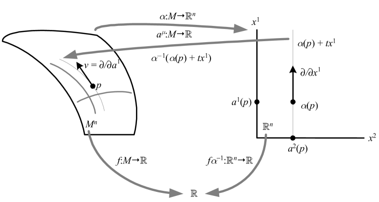
Figure B.2: In a particular coordinate chart, a tangent vector $v$ operates on a function by taking the derivative of the composite function in $\mathbb{R}^{n}$ in the direction of $v^{\mu}\partial/\partial a^{\mu}$.

Thus at a point $p$, we have

$$v^{\mu}\frac{\partial}{\partial a^{\mu}}\left(f\right)=v^{\mu}\frac{\partial}{\partial x^{\mu}}\left(f\circ\alpha^{-1}\left(x\right)\right),$$ (B.2)

where $x=\alpha(p)$. The coordinate line $\alpha^{-1}\left(a^{\mu}\left(p\right)+tv^{\mu}x^{\mu}\right)$ is a parameterized curve on $M$, and thus it and the tangent vector itself are coordinate-independent objects. In this chart, any parametrized curve is defined to have tangent $v$ at $t=0$ if its coordinates are $C^{\mu}\left(t\right)\equiv a^{\mu}+tv^{\mu}$ to first order in $t$; therefore the coordinates of the tangent vector to $C$ at any point may be obtained by

$$v^{\mu}=\frac{\mathrm{d}C^{\mu}}{\mathrm{d}t}.$$ (B.3)

In another coordinate chart, the coordinate line that yields the same operator on functions near $p$ can be seen to correspond to the familiar transformation of vector components

$$v=v^{\mu}\frac{\partial}{\partial a^{\mu}}=\left(v^{\lambda}\frac{\partial b^{\mu}}{\partial a^{\lambda}}\right)\frac{\partial}{\partial b^{\mu}}.$$ (B.4)

We can consider the point “$p$ moved in the direction $v$” by abusing notation to write $p^{\mu}+tv^{\mu}$ in place of $\alpha^{-1}\left(a^{\mu}\left(p\right)+tv^{\mu}x^{\mu}\right)$; this is a coordinate-dependent expression, but in the limit $\varepsilon\rightarrow 0$ we can unambiguously write $p+\varepsilon v$ to refer to the concept “$p$ moved infinitesimally in the direction $v$,” which is coordinate-independent. This allows us to write

$$v(f)=\underset{\varepsilon\rightarrow 0}{\textrm{lim}}\frac{1}{\varepsilon}\left[f_{p+\varepsilon v}-f_{p}\right].$$ (B.5)

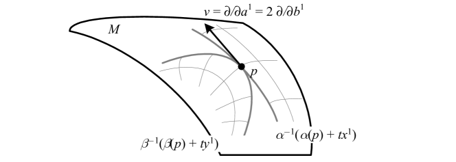
Figure B.3: A tangent vector $v$ in terms of two different coordinate charts. $v^{\mu}=(1,0)$ in chart $\alpha$ with coordinate functions $a^{\mu}\left(p\right)=x^{\mu}$, and $v^{\mu}=\left(2,0\right)$ in chart $\beta$ with coordinate functions $b^{\mu}\left(p\right)=y^{\mu}$. The divergent coordinate lines show that the concept of moving a point “in the direction of $v$” can only be coordinate-independent in the infinitesimal limit.

The set of all tangent spaces in a region $U$ is called the tangent bundle, and is denoted $TU$. A (smooth, contravariant) vector field on $U$ is then a tangent vector defined at each point such that its application to a smooth function on $U$ is again smooth. Similarly, a covariant vector field is a $1$-form defined at each point such that its value on a vector field is a smooth function, and a tensor field is the tensor product of vector fields and covariant vector fields.

$\triangle$ Tensor fields (including vector fields and covariant vector fields) are written using the same notation as tensors, making it important to distinguish the two situations. In particular, one can define a (pseudo) metric tensor field, which is then usually referred to as simply a metric.

Note that a tensor field must remain a tensor locally at any point $p$, i.e. it must be a multi-linear mapping. For example, a covariant tensor field can only depend upon the values of its vector field arguments at $p$, since otherwise one could add a vector field that vanishes at $p$ and obtain a different result. This means that operators such as the derivatives on manifolds we will see in Sections C and 2 cannot usually be viewed as tensors, since they measure the difference between arguments at different points.

Since vectors are operators on functions, we can apply one vector field to another. Following the practice of using $\partial/\partial x^{u}$ to refer to $\partial/\partial a^{\mu}$, this can be used to define the Lie bracket of vector fields

$$\left[v,w\right](f) \equiv v(w(f))-w(v(f))$$ (B.6)

$$\Rightarrow\left[v,w\right] =\left(v^{\mu}\frac{\partial w^{\lambda}}{\partial x^{\mu}}-w^{\mu}\frac{\partial v^{\lambda}}{\partial x^{\mu}}\right)\frac{\partial}{\partial x^{\lambda}}.$$

Here we have used the equality of mixed partials, and can easily verify that $\left[v,w\right]$ is anti-commuting and satisfies the Jacobi identity. Since this expression is coordinate-independent, $\left[v,w\right]$ is a vector field and we can thus view $\textrm{vect}\left(M\right)$, the set of all vector fields on $M$, as the infinite-dimensional Lie algebra of vector fields on $M$, with vector multiplication defined by the Lie bracket.

Having defined vector and tensor fields on manifolds, we can now define a differential form as an alternating covariant tensor field, i.e. an exterior form in $\Lambda\left(T_{p}U\right)$ smoothly defined for every point $p$.

$\triangle$ Just as tensor fields are usually referred to as simply tensors, differential forms are usually referred to as simply forms, and a $k$-form is written simply $\varphi\in\Lambda^{k}M$. It is important to remember that in the context of manifolds, a $k$-form is an exterior form smoothly defined on $k$ elements of the tangent space at each point, i.e. an anti-symmetric covariant $k$-tensor field.

On a differentiable manifold, the existence of $k$-forms makes possible a more concrete definition of orientability: a manifold $M^{n}$ is orientable if there exists a non-vanishing $n$-form. Such a form is called a volume form (AKA volume element), since it gains a Jacobian-like determinant factor under invertible linear transformations.

$\triangle$ The term “volume form” or “volume element” is sometimes defined in physics to reflect the intuitive idea of a form which returns the volume spanned by its argument vectors; however, volume is always positive, so that in this usage we are more accurately referring to a volume pseudo-form whose value is the absolute value of the volume form as we have defined it, and which exists on any differentiable manifold, including those which are non-orientable.

B.3 Frames

A frame $e_{\mu}$ on $U\subset M^{n}$ is defined to be a tensor field of bases for the tangent spaces at each point, i.e. $n$ linearly independent smooth vector fields $e_{\mu}$.

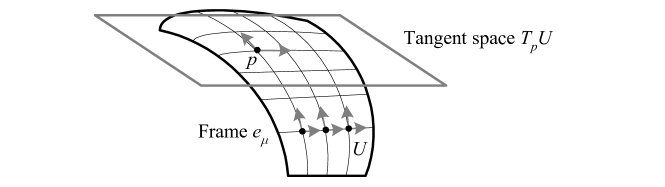
Figure B.4: A frame $e_{\mu}$ is $n$ smooth vector fields that together provide a basis for the tangent space at every point.

The concept of frame has a particularly large number of synonyms, including comoving frame, repère mobile, vielbein, $n$-frame, and $n$-bein (where $n$ is the dimension). The dual frame, the $1$-forms $\beta^{\mu}$ corresponding to a frame $e_{\mu}$, is also often simply called the frame.

When using particular coordinates $x^{\mu}$, the frame $e_{\mu}=\partial/\partial x^{\mu}$ is called the coordinate frame (AKA coordinate basis or associated basis); any other frame is then called a non-coordinate frame. A holonomic frame is a coordinate frame in some coordinates (though perhaps not the ones being used); this condition is equivalent to requiring that $\left[e_{\mu},e_{\nu}\right]=0$, a result which is sometimes called Frobenius’ theorem. An anholonomic frame is then a frame that cannot be derived from any coordinate chart in its region of definition. Using a non-coordinate frame suited to a specific problem is sometimes called the method of moving frames.

$\triangle$ Note that the distinction between holonomic and coordinate frames as defined here is often not made.

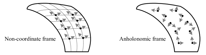
Figure B.5: A non-coordinate frame is not tangent to the coordinate functions being used, while an anholonomic frame cannot be derived from any coordinate chart.

A frame cannot usually be globally defined on a manifold. A simple way to see this is by the example of the 2-sphere $S^{2}$. Any drawing of coordinate functions on a globe will have singularities, such as the north and south poles when using latitude and longitude; these are points where the associated coordinate frame will either be undefined or will vanish. In general, there is no non-zero smooth vector field that can be defined on $S^{n}$ for even $n$ (this is sometimes called the hedgehog theorem, AKA hairy ball theorem, coconut theorem).

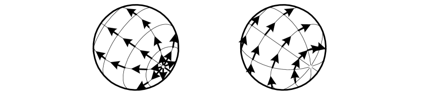
Figure B.6: The hedgehog theorem for $S^{2}$, showing that any attempt to “comb the hair of a hedgehog” yields bald spots, in this case at the poles.

A manifold that can have a global frame defined on it is called parallelizable. Some facts regarding parallelizable manifolds include:

• All parallelizable manifolds are orientable (and therefore have a volume form), but as we saw with $S^{2}$ the converse is not in general true

• Any orientable 3-manifold $M^{3}$ is parallelizable $\Rightarrow$ any 4-manifold $M^{3}\times\mathbb{R}$ is parallelizable (important in the case of the spacetime manifold)

• Of the $n$-spheres, only $S^{1}$, $S^{3}$, and $S^{7}$ are parallelizable (this can be seen to be related to $\mathbb{C}$, $\mathbb{H}$, and $\mathbb{O}$ being the only normed finite-dimensional real division algebras beyond $\mathbb{R}$)

• The torus (with any number of holes) is the only closed orientable surface with a non-zero smooth vector field

B.4 Tangent vectors in terms of frames

It is important to remember that in following our intuitive picture of a Euclidean surface, our central definitions were manifolds $M$ and tangent vectors $v$. These are the “real” intrinsic objects, while their expressions in terms of a particular coordinate chart and frame are arbitrary. Coordinates and frames are “temporary” tools we use to “componentize” points and tangents on a manifold.

In particular, if a manifold is defined in terms of a set of coordinate functions that feature a singularity, this singularity may be due to the coordinates extending outside of their valid chart, telling us nothing about whether the manifold itself has a singularity. Every point of a well-defined differentiable manifold always has a local coordinate chart and tangent vectors.

For example, given the typical spherical coordinate chart for $S^{2}$ the associated frame will be singular at the poles, since they are outside of $U$ for that chart; nevertheless, tangent vectors are well-defined at these points, and can be expressed perfectly normally in a different chart.

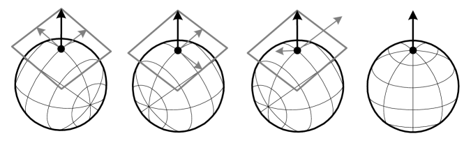
Figure B.7: A manifold and tangent vector expressed in terms of different coordinate functions and frames.

In the above figure, we see the following situations depicted:

• $v=e_{1}+e_{2}=\partial/\partial x^{1}+\partial/\partial x^{2}$ (expressed in a coordinate frame)

• $v=e_{1}^{\prime}-e_{2}^{\prime}=\partial/\partial x^{\prime 1}-\partial/\partial x^{\prime 2}$ (using a different coordinate frame)

• $v=e_{1}^{\prime\prime}+3e_{2}^{\prime\prime}=\partial/\partial x^{\prime 1}-\partial/\partial x^{\prime 2}$ (in a non-coordinate frame)

The final figure depicts coordinate functions that are singular at the point of interest; the manifold and vector are still well-defined, but the tangent space at this point cannot be expressed in terms of this coordinate chart.

$\triangle$ In general, when working with objects on manifolds, it is important to keep clearly in mind whether a given symbol represents a vector, form, or function (0-form); whether any given index is a label, an abstract index or a component index in a particular frame or coordinates; and whether the object is a field with a value at each point, or is only valid at a particular point. Any calculation can always be made explicit by expressing everything in terms of functions and differential operators on them.

B.5 Diffeomorphisms

In the same way that spaces or topological manifolds are equivalent if they are related by a homeomorphism, differentiable manifolds are equivalent if they are related by a diffeomorphism, a homeomorphism that is differentiable along with its inverse. As usual we define differentiability by moving the mapping to $\mathbb{R}^{n}$, e.g. $\Phi\colon M\to N$ is differentiable if $\alpha_{N}\circ\Phi\circ\alpha_{M}^{-1}\colon\mathbb{\mathbb{R}}^{m}\to\mathbb{R}^{n}$ is, where $\alpha_{M}$ and $\alpha_{N}$ are charts for $M$ and $N$. Intuitively, a diffeomorphism like a homeomorphism can be thought of as arbitrary stretching and bending, but it is “nicer” in that it preserves the differentiable structure.

$\triangle$ It is important to distinguish between coordinate transformations, which are locally defined and so may have singularities outside of a given region; and diffeomorphisms, which are globally defined and form a group. One can define a coordinate transformation on a region of a manifold that avoids any resulting singularities, but a diffeomorphism must be smooth on the entire manifold.

B.6 The differential and pullback

If we consider a general mapping between manifolds $\Phi\colon M^{m}\to N^{n}$, we can choose charts $\alpha_{M}\colon M\to\mathbb{R}^{m}$ and $\alpha_{N}\colon N\to\mathbb{R}^{n}$, with coordinate functions $x^{\mu}$ and $y^{\nu}$, so that the mapping $\alpha_{N}\circ\Phi\colon M\to\mathbb{R}^{n}$ can be represented by $n$ functions $\Phi^{\nu}\colon M\to\mathbb{R}$. This allows us to write down an expression for the induced tangent mapping or differential (aka pushforward, derivative) $\mathrm{d}\Phi\colon TM\to TN$ (also denoted $T\Phi$ or $\Phi_{*}$ or sometimes simply $\Phi$ if it is clear the argument is a tangent vector). For a tangent vector $v=v^{\mu}\partial/\partial x^{\mu}$ at a point $p\in M$ we define

$$\left.\mathrm{d}\Phi\left(v\right)\right|_{p}\equiv\left.v^{\mu}\frac{\partial\Phi^{\nu}}{\partial x^{\mu}}\frac{\partial}{\partial y^{\nu}}\right|_{\Phi\left(p\right)}.$$ (B.7)

This definition can be shown to be coordinate-independent and to follow our intuitive expectation that mapped tangent vectors stay tangent to mapped curves. If $M=N$ and $\Phi$ is the identity, $\mathrm{d}\Phi$ is just the vector component transformation in Section B.2. The matrix

$$J_{\Phi}(x)\equiv\frac{\partial\Phi^{\nu}}{\partial x^{\mu}}$$ (B.8)

is called the Jacobian matrix (AKA Jacobian). For the parametrized curve $C\colon\mathbb{R}\to N^{n}$, we define the tangent to the curve at $t\in\mathbb{R}$ to be

$$\dot{C}\left(t\right) \equiv\left.\mathrm{d}C\left(\frac{\partial}{\partial x}\right)\right|_{t}$$ (B.9)

$$=\left.\frac{\partial C^{\lambda}}{\partial x}\frac{\partial}{\partial y^{\lambda}}\right|_{C\left(t\right)},$$

which is also denoted $\frac{\mathrm{d}C\left(t\right)}{\mathrm{d}t}$ and coincides with the Euclidean tangent to a curve if $N=\mathbb{R}^{n}$.

If $\Phi$ is a diffeomorphism, $\mathrm{d}\Phi$ is an isomorphism between the tangent spaces at every point in $M$. The inverse function theorem says that the converse is true locally: if $\mathrm{d}\Phi_{p}$ is an isomorphism at $p\in M$, then $\Phi$ is locally a diffeomorphism. In particular, this means that if in some coordinates the Jacobian matrix is nonsingular, then $\alpha_{N}\circ\Phi\circ\alpha_{M}^{-1}$ represents a locally valid coordinate transformation and $\Phi^{\nu}=y^{\nu}$.

A mapping between manifolds $\Phi\colon M^{m}\to N^{n}$ also can be used to naturally define the pullback of a form $\Phi^{*}\colon\Lambda^{k}N\to\Lambda^{k}M$ by

$$\Phi^{*}\varphi\left(v_{1},\dotsc,v_{k}\right)=\varphi\left(\mathrm{d}\Phi\left(v_{1}\right),\dotsc,\mathrm{d}\Phi\left(v_{k}\right)\right),$$ (B.10)

where the name indicates that a form on $N$ can be “pulled back” to $M$ using $\Phi$. Note that the composition of pullbacks is then

$$\Psi^{*}\Phi^{*}\varphi=(\Phi\Psi)^{*}\varphi.$$ (B.11)

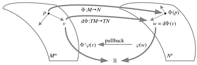
Figure B.8: Forms $\varphi$ on $N$ are pulled back to $M$ by sending argument vectors to $N$ using $\mathrm{d}\Phi$.

Note that for a mapping $f\colon M\to\mathbb{R}$, we have $\mathrm{d}f\colon TM\to T\mathbb{R}\cong\mathbb{R}$, so that $\mathrm{d}f\left(v\right)=v^{\mu}\partial f/\partial x^{\mu}=v\left(f\right)$, the directional derivative of $f$. Let us apply this to the coordinate function $x^{1}\colon M\to\mathbb{R}$. Then we have $\mathrm{d}x^{1}\left(v\right)=v^{\mu}\partial x^{1}/\partial x^{\mu}=v^{1}$, so that in particular $\mathrm{d}x^{\nu}\left(\partial/\partial x^{\mu}\right)=?\delta^{\nu}{}_{\mu}?$, i.e. $\mathrm{d}x^{\mu}$ is in fact the dual frame to $\partial/\partial x^{\mu}$. Thus in a given coordinate system, we can write a general tensor of type $(m,n)$ as

$$T=?T^{\mu_{1}\dots\mu_{m}}{}_{\nu_{1}\dots\nu_{n}}?\frac{\partial}{\partial x^{\mu_{1}}}\otimes\dotsb\otimes\frac{\partial}{\partial x^{\mu_{m}}}\otimes\mathrm{d}x^{\nu_{1}}\otimes\dotsb\otimes\mathrm{d}x^{\nu_{n}}.$$ (B.12)

In particular, the metric tensor is often written

$$\mathrm{d}s^{2}\equiv g=g_{\mu\nu}\mathrm{d}x^{\mu}\mathrm{d}x^{\nu},$$ (B.13)

where the Einstein summation convention is used and the tensor symbol omitted. A general $k$-form $\varphi\in\Lambda^{k}M$ can then be written as

$$\varphi=\underset{\mu_{1}<\dotsb<\mu_{k}}{\sum}\varphi_{\mu_{1}\dots\mu_{k}}\mathrm{d}x^{\mu_{1}}\wedge\dotsb\wedge\mathrm{d}x^{\mu_{k}}.$$ (B.14)

From either the tangent mapping definition or the behavior of the exterior product under a change of basis, we can see that under a change of coordinates we have

$$\mathrm{d}y^{\mu_{1}}\wedge\dotsb\wedge\mathrm{d}y^{\mu_{k}}=\textrm{det}\left(\frac{\partial y^{\nu}}{\partial x^{\mu}}\right)\mathrm{d}x^{\mu_{1}}\wedge\dotsb\wedge\mathrm{d}x^{\mu_{k}}.$$ (B.15)

This is the familiar Jacobian determinant (like the Jacobian matrix, also often called the Jacobian) that appears in the change of coordinates rule for integrals from calculus, and explains the name of the volume form as defined previously in terms of the exterior product.

In summary, the differential $\mathrm{d}$ has a single definition, but is used in several different settings that are not related in an immediately obvious way.

Construct	Argument	Other names	Other symbols
$\mathrm{d}\Phi\colon TM\to TN$	$\Phi\colon M\to N$	Tangent mapping	$T\Phi$, $\Phi_{*}$, $\Phi$
$\mathrm{d}f\colon TM\to\mathbb{R}$	$f\colon M\to\mathbb{R}$	Directional derivative	$v\left(f\right)$, $\mathrm{d}_{v}f$, $\nabla_{v}f$
$\mathrm{d}x^{\mu}\colon TM\to\mathbb{R}$	$x^{\mu}\colon M\to\mathbb{R}$	Dual frame to $\partial/\partial x^{\mu}$	$\beta^{\mu}$

Table B.1: Various uses of the differential on manifolds.

B.7 Immersions and embeddings

We can generalize and make precise the concept of a surface embedded in 3-dimensional space with the following definitions concerning a differentiable map $\Phi\colon M^{m}\to N^{n}$:

• Immersion: $\mathrm{d}\Phi$ is injective for all $p\in M$; intuitively, a smooth mapping that doesn’t collapse the tangent spaces

• Submanifold: an immersion with $\Phi$ injective; intuitively, an immersion that doesn’t intersect itself

• Embedding (AKA imbedding): a submanifold with $\Phi$ a homeomorphism onto $\Phi\left(M\right)$; intuitively, a submanifold that doesn’t have intersecting limit points

Figure B.9: $\mathbb{R}$ immersed in $\mathbb{R}^{2}$; the second immersion approaches a self-intersection in the limit as the line approaches infinity.

The difference in dimension $\left(n-m\right)$ is called the codimension of the embedding. The Whitney embedding theorem states that for positive codimension, any $M^{m}$ can be immersed in $\mathbb{R}{}^{(2m-1)}$ and embedded in $\mathbb{R}^{2m}$. Thus we can view differentiable manifolds as generalized surfaces that we study without making reference to the enclosing Euclidean space. The limiting dimension of this theorem is illustrated by noting that the real projective space $\mathbb{R}\textrm{P}^{m}$ cannot be embedded in $\mathbb{R}^{(2m-1)}$.

Appendix C Derivatives on manifolds

In this section we will introduce various objects that in some way measure how vectors or forms change from point to point on a manifold.

C.1 Derivations

In general, we define a derivation to be a linear map $\mathcal{D}\colon\mathfrak{a}\to\mathfrak{a}$ on an algebra $\mathfrak{a}$ that follows the Leibniz rule (AKA product rule)

$$\mathcal{D}(AB)=(\mathcal{D}A)B+A(\mathcal{D}B).$$ (C.1)

As noted previously in Section B.2, the set $\mathrm{vect}(M)$ of vector fields on a manifold form a Lie algebra; the Lie bracket operation with a fixed vector field $\left[u,\;\right]$ is then a derivation on this algebra, since the Leibniz rule

$$\left[u,\left[v,w\right]\right]=\left[\left[u,v\right],w\right]+\left[v,\left[u,w\right]\right]$$ (C.2)

is just the Jacobi identity.

For a graded algebra, e.g. the exterior algebra, the degree of a derivation is the integer $c$ where $\mathcal{D}\colon\Lambda^{k}M\to\Lambda^{k+c}M$. A graded derivation is defined to follow the graded Leibniz rule, e.g. for a $k$-form $\varphi$,

$$\mathcal{D}\left(\varphi\wedge\psi\right)=\mathcal{D}\varphi\wedge\psi+\left(-1\right)^{kc}\varphi\wedge\mathcal{D}\psi.$$ (C.3)

If $c$ is odd, a graded derivation is sometimes called an anti-derivation (AKA skew-derivation).

C.2 The Lie derivative of a vector field

Without some kind of additional structure, there is no way to “transport” vectors, or compare them at different points on a manifold, and therefore no way to construct a vector derivative. The simplest way to introduce this structure is via another vector field, which leads us to the Lie derivative

$$L_{v}w\equiv\left[v,w\right].$$ (C.4)

As noted above, $L_{v}$ is a derivation due to the Jacobi identity. In this section we define the Lie derivative in terms of infinitesimal vector transport, and explore its geometrical meaning.

Given any vector field $v$ on $M$, it can be shown ([2] pp. 125-127) that there exists a parameterized curve $v_{p}(t)$ at every point $p\in M$ such that $v_{p}(0)=p$ and $\dot{v}_{p}(t)$ is the value of the vector field $v$ at the point $v_{p}(t)$ (the dot indicates the derivative with respect to $t$, which as usual is calculated on the curve mapped to $\mathbb{R}^{n}$ by the coordinate chart). Each curve in this family is in general only well-defined locally, i.e. for $-\varepsilon<t<\varepsilon$, and is thus called the local flow of $v$.

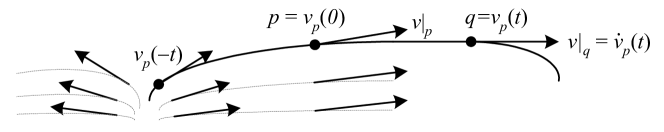
Figure C.1: A depiction of the local flow of a vector field $v$, with details on the local parameterized curve $v_{p}(t)$ at a point $p$.

For a fixed value of $t$, there is some region $U\subset M$ where the map $\Phi_{t}\colon U\to U$ defined by $p\mapsto v_{p}\left(t\right)$ is a diffeomorphism, and within the valid domain of $t$ the maps $\Phi_{t}$ satisfy the abelian group law $\Phi_{t}\circ\Phi_{s}=\Phi_{t+s}$; thus the $\Phi_{t}$ are called a local one-parameter group of diffeomorphisms. This name is somewhat misleading, since due to the limited domain of $t$ the maps $\Phi_{t}$ do not actually form a group; the “local” reflects the fact that the diffeomorphisms are not on all of $M$. In the case that these maps are in fact valid for all of $t$ and $M$, $v$ is called a complete vector field, and the $\Phi_{t}$ are called a one-parameter group of diffeomorphisms. If $M$ is compact, then every vector field is complete; if not, then a vector field is complete if it has compact support (is non-zero on a compact subset of $M$).

The tangent map $\mathrm{d}\Phi$ defined by the vector field $v$ is then the extra structure we need to “transport” vectors. $\mathrm{d}\Phi$ maps a vector tangent to the curve $C$ to a vector tangent to the curve $\Phi\left(C\right)$; it “pushes vectors along the flow of $v$.” We can now define the Lie derivative as a limit

$$L_{v}w \equiv\underset{\varepsilon\rightarrow 0}{\textrm{lim}}\frac{1}{\varepsilon}\left[\mathrm{d}\Phi_{-\varepsilon}\left(w\left|{}_{v_{p}\left(\varepsilon\right)}\right.\right)-w\left|{}_{p}\right.\right]$$ (C.5)

$$=\underset{\varepsilon\rightarrow 0}{\textrm{lim}}\frac{1}{\varepsilon}\left[w\left|{}_{v_{p}\left(\varepsilon\right)}\right.-\mathrm{d}\Phi_{\varepsilon}\left(w\left|{}_{p}\right.\right)\right]$$

$$=\underset{\varepsilon\rightarrow 0}{\textrm{lim}}\frac{1}{\varepsilon}\left[w\left|{}_{p}\right.-\mathrm{d}\Phi_{\varepsilon}\left(w\left|{}_{v_{p}\left(-\varepsilon\right)}\right.\right)\right].$$

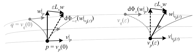
Figure C.2: The Lie derivative $L_{v}w$ is “the difference between $w$ and its transport by the local flow of $v$.”

☼ In this and future depictions of vector derivatives, the situation is simplified by focusing on the change in the vector field $w$ while showing the “transport” of $w$ as a parallel displacement. This has the advantage of highlighting the equivalency of defining the derivative at either 0 or $\varepsilon$ in the limit $\varepsilon\rightarrow 0$. Depicting $L_{v}w$ as a non-parallel vector at $v_{p}\left(t\right)$ would be more accurate, but would obscure this fact. We also will follow the picture here in using words to characterize derivatives: namely, “the difference” is short for “the difference per unit $\varepsilon$ to order $\varepsilon$ in the limit $\varepsilon\rightarrow 0$.”

This definition can be shown to be equivalent to $L_{v}w\equiv\left[v,w\right]$. Another way of depicting the Lie derivative that highlights the anti-commutativity of the Lie bracket is to consider $L_{v}w$ in terms of a loop defined by the flows of $v$ and $w$.

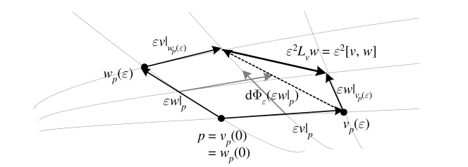
Figure C.3: The Lie derivative $L_{v}w$ can also be pictured as the vector field whose local flow is the “commutator of the flows of $v$ and $w$,” i.e. it is the difference between the local flow of $v$ followed by $w$ and that of $w$ followed by $v$. Thus $L_{v}w$ “completes the parallelogram” formed by the flow lines.

C.3 The Lie derivative of an exterior form

The Lie derivative $L_{v}$ can be applied to a $k$-form $\varphi$ by using the pullback of $\varphi$ by the diffeomorphism $\Phi$ associated with the flow of $v$, i.e. applied to $k$ vectors $w_{1},\ldots,w_{k}$ we define

$$L_{v}\varphi\left(w_{1},\ldots,w_{k}\right)\equiv\underset{\varepsilon\rightarrow 0}{\textrm{lim}}\frac{1}{\varepsilon}\left[\varphi\left(\mathrm{d}\Phi_{\varepsilon}\left(w_{1},\ldots,w_{k}\right)\right)-\varphi\left(w_{1},\ldots,w_{k}\right)\right].$$ (C.6)

$L_{v}\varphi$ thus measures the change in $\varphi$ as its arguments are transported by the local flow of $v$. In the case of a 0-form $f$, this is just the differential or directional derivative $L_{v}f=v(f)=\mathrm{d}f(v)$.

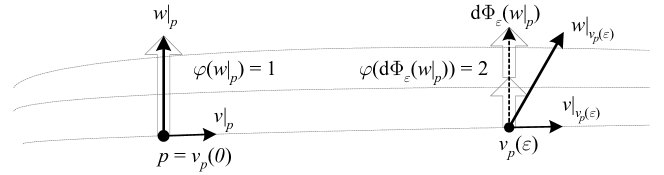
Figure C.4: The Lie derivative illustrated for a 1-form $\varphi$ with $\varepsilon=1$. $L_{v}\varphi$ is “the difference between $\varphi$ applied to $w$ and $\varphi$ applied to $w$ transported by the local flow of $v$,” so above we have $L_{v}\varphi(w)=2-1=1$ (valid in the limit $\varepsilon\rightarrow 0$ if $\varphi$ changes linearly in the range shown).

By using the above definitions of the Lie derivative applied to vectors and 1-forms, and noting that we can derive a Leibniz rule over contraction $L_{v}(\varphi\left(w\right))=\left(L_{v}\varphi\right)(w)+\varphi\left(L_{v}w\right)$, we arrive at an expression for the Lie derivative applied to general tensors, viewed as real-valued mappings on vectors and 1-forms:

$$L_{v}T(\varphi_{1},\ldots,\varphi_{m},w_{1},\ldots,w_{n}) =v\left(T(\varphi_{1},\ldots,\varphi_{m},w_{1},\ldots,w_{n})\right)$$ (C.7)

$$-\sum_{j=1}^{m}T\left(\varphi_{1},\ldots,L_{v}\varphi_{j},\ldots,\varphi_{m},w_{1},\ldots,w_{n}\right)$$

$$-\sum_{j=1}^{n}T\left(\varphi_{1},\ldots,\varphi_{m},w_{1},\ldots,L_{v}w_{j},\ldots,w_{n}\right)$$

In a holonomic frame, this yields an expression for the Lie derivative of a tensor in terms of coordinates

$$L_{v}?T^{\mu_{1}\dots\mu_{m}}{}_{\sigma_{1}\dots\sigma_{n}}? =v^{\lambda}\frac{\partial}{\partial x^{\lambda}}?T^{\mu_{1}\dots\mu_{m}}{}_{\sigma_{1}\dots\sigma_{n}}?$$ (C.8)

$$-\sum_{j=1}^{m}\left(\frac{\partial v^{\mu_{j}}}{\partial x^{\lambda}}\right)?T^{\mu_{1}\dots\mu_{j-1}\lambda\mu_{j+1}\dots\mu_{m}}{}_{\sigma_{1}\dots\sigma_{n}}?$$

$$+\sum_{j=1}^{n}\left(\frac{\partial v^{\lambda}}{\partial x^{\sigma_{j}}}\right)?T^{\mu_{1}\dots\mu_{m}}{}_{\sigma_{1}\dots\sigma_{j-1}\lambda\sigma_{j+1}\dots\sigma_{n}}?.$$

From this we can confirm that the Lie derivative satisfies the Leibniz rule over the tensor product, and therefore is a derivation of degree 0 on both the tensor algebra and the exterior algebra.

C.4 The exterior derivative of a 1-form

The Lie derivative $L_{v}\varphi$ is defined in terms of a vector field $v$, and its value as a “change in $\varphi$” is computed by using $v$ to transport the arguments of $\varphi$. In contrast, recall that the differential $\mathrm{d}$ takes a 0-form $f\colon M\to\mathbb{R}$ to a 1-form $\mathrm{d}f\colon TM\to\mathbb{R}$ with

$$\mathrm{d}f(v)=v(f).$$ (C.9)

Thus $\mathrm{d}$ is a derivation of degree +1 on 0-forms, whose value as a “change in $f$” is computed using the vector field argument of the resulting 1-form.

We would like to generalize $\mathrm{d}$ to $k$-forms by extending this idea of including the “direction argument” by increasing the degree of the form. It turns out that if we also require the property

$$\mathrm{d}\left(\mathrm{d}\left(\varphi\right)\right)=0$$ (C.10)

(or “$\mathrm{d}^{2}=0$”), there is a unique graded derivation of degree +1 that extends $\mathrm{d}$ to general $k$-forms; this derivation is called the exterior derivative. We first explore the exterior derivative of a 1-form.

The exterior derivative of a 1-form is defined by

$$\mathrm{d}\varphi\left(v,w\right)\equiv v\left(\varphi\left(w\right)\right)-w\left(\varphi\left(v\right)\right)-\varphi\left(\left[v,w\right]\right),$$ (C.11)

where e.g.

$$v\left(\varphi\left(w\right)\right)=\underset{\varepsilon\rightarrow 0}{\textrm{lim}}\frac{1}{\varepsilon}\left[\varphi\left(w\left|{}_{v_{p}\left(\varepsilon\right)}\right.\right)-\varphi\left(w\left|{}_{p}\right.\right)\right]$$ (C.12)

measures the change in $\varphi\left(w\right)$ in the direction $v$, so that

$$\mathrm{d}\varphi\left(v,w\right) =\underset{\varepsilon\rightarrow 0}{\textrm{lim}}\frac{1}{\varepsilon^{2}}\left[\left(\varphi\left(\varepsilon w\left|{}_{v_{p}\left(\varepsilon\right)}\right.\right)-\varphi\left(\varepsilon w\left|{}_{p}\right.\right)\right)\right.$$ (C.13)

$$\phantom{{=\underset{\varepsilon\rightarrow 0}{\textrm{lim}}\frac{1}{\varepsilon^{2}}\left[-\right.}}-\left(\varphi\left(\varepsilon v\left|{}_{w_{p}\left(\varepsilon\right)}\right.\right)-\varphi\left(\varepsilon v\left|{}_{p}\right.\right)\right)$$

$$\phantom{{=\underset{\varepsilon\rightarrow 0}{\textrm{lim}}\frac{1}{\varepsilon^{2}}\left[-\right.}}\left.-\varphi\left(\varepsilon^{2}\left[v,w\right]\right)\right].$$

The term involving the Lie bracket “completes the parallelogram” formed by $v$ and $w$, so that $\mathrm{d}\varphi\left(v,w\right)$ can be viewed as the “sum of $\varphi$ on the boundary of the surface defined by its arguments.”

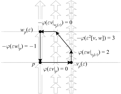
Figure C.5: The exterior derivative of a 1-form $\mathrm{d}\varphi\left(v,w\right)$ is the sum of $\varphi$ along the boundary of the completed parallelogram defined by $v$ and $w$. So if in the diagram $\varepsilon=1$, we have $\mathrm{d}\varphi\left(v,w\right)=\left(2-1\right)-\left(0-0\right)+3=4$. This value is valid in the limit $\varepsilon\rightarrow 0$ if the sum varies like $\varepsilon^{2}$ as depicted in the figure.

The identity $\mathrm{d}^{2}=0$ can then be seen as stating the intuitive fact that the boundary of a boundary is zero. If $\varphi=\mathrm{d}f$, then $\varphi\left(v\right)=\mathrm{d}f\left(v\right)=v\left(f\right)$, the change in $f$ along $v$. Thus e.g. $\varepsilon\varphi\left(v\left|{}_{p}\right.\right)=f\left(v_{p}\left(\varepsilon\right)\right)-f\left(p\right)$, so that the value of $\varphi$ on $v$ is the difference between the values of $f$ on the two points which are the boundary of $v$. Each endpoint will be cancelled by a starting point as we add up values of $\varphi$ along a sequence of vectors, resulting in the difference between the values of $f$ at the boundary of the total path defined by these vectors. $\mathrm{d}\varphi$ is the value of $\varphi$ over the boundary path of the surface defined by its arguments, which has no boundary points and so vanishes.

Figure C.6: $\mathrm{d}^{2}=0$ corresponds to the boundary of a boundary is zero: each term $\varphi(v)=\mathrm{d}f(v)$ is the difference between the values of $f$ on the boundary points of $v$, which cancel as we traverse the boundary of the surface defined by the arguments of $\mathrm{d}\varphi(v,w)$. In the figure we assume a vanishing Lie bracket for simplicity.

Note that $\mathrm{d}\varphi\left(v,w\right)$ measures the interaction between $\varphi$ and the vector fields $v$ and $w$, thus avoiding the need to “transport” vectors. In particular, a non-zero exterior derivative can be pictured as resulting from either the vector fields or $\varphi$ “changing,” i.e. changing with regard to the implied coordinates of our pictures.

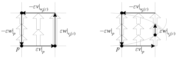
Figure C.7: A non-zero exterior derivative $\mathrm{d}\varphi\left(v,w\right)$ results from changes in $\varphi\left(v\right)$ or $\varphi\left(w\right)$, not changes in either $\varphi$ or the vector fields alone as compared to some transport.

If we calculate $\mathrm{d}\varphi\left(e_{1},e_{2}\right)$ explicitly in a holonomic frame in two dimensions, $\mathrm{d}\left(\varphi_{1}\mathrm{d}x^{1}+\varphi_{2}\mathrm{d}x^{2}\right)=\mathrm{d}\varphi_{1}\wedge\mathrm{d}x^{1}+\mathrm{d}\varphi_{2}\wedge\mathrm{d}x^{2}$, so applying this to the basis vector fields $e_{1}$ and $e_{2}$ we have

$$\mathrm{d}\varphi\left(e_{1},e_{2}\right) =\mathrm{d}\varphi_{1}\left(e_{1}\right)\cdot\mathrm{d}x^{1}\left(e_{2}\right)-\mathrm{d}\varphi_{1}\left(e_{2}\right)\cdot\mathrm{d}x^{1}\left(e_{1}\right)$$ (C.14)

$$\phantom{{}=}+\mathrm{d}\varphi_{2}\left(e_{1}\right)\cdot\mathrm{d}x^{2}\left(e_{2}\right)-\mathrm{d}\varphi_{2}\left(e_{2}\right)\cdot\mathrm{d}x^{2}\left(e_{1}\right)$$

$$=e_{1}\left(\varphi_{2}\right)-e_{2}\left(\varphi_{1}\right)$$

$$=\frac{\partial\varphi_{2}}{\partial x^{1}}-\frac{\partial\varphi_{1}}{\partial x^{2}}.$$

Note that a holonomic dual frame $\beta^{\mu}=\mathrm{d}x^{\mu}$ satisfies $\mathrm{d}\beta^{\mu}=\mathrm{dd}x^{\mu}=0$.

C.5 The exterior derivative of a k-form

The extension of the coordinate-free definition of $\mathrm{d}$ to general $k$-forms gives the expression

$$\mathrm{d}\varphi\left(v_{0},\dotsc,v_{k}\right)$$ (C.15)

$$\equiv\sum_{j=0}^{k}\left(-1\right)^{j}v_{j}\left(\varphi\left(v_{0},\dotsc,v_{j-1},v_{j+1},\dotsc,v_{k}\right)\right)$$

$$\phantom{{}=}+\sum_{i<j}\left(-1\right)^{i+j}\varphi\left(\left[v_{i},v_{j}\right],v_{0},\dotsc,v_{i-1},v_{i+1},\dotsc,v_{j-1},v_{j+1},\dotsc,v_{k}\right).$$

Our picture of $\mathrm{d}^{2}=0$ for 1-forms then can be extended to higher dimensions. For example, assuming vanishing Lie brackets to simplify the picture, the exterior derivative of a 2-form $\mathrm{d}\varphi\left(u,v,w\right)$ can be viewed as the “sum of $\varphi$ on the boundary faces of the cube defined by its arguments.” If $\varphi=\mathrm{d}\psi\left(v,w\right)$ is the boundary of a face, $\mathrm{d}\varphi=\mathrm{d}^{2}\psi$ is the sum of the boundaries of the faces; each edge is then counted by two faces with opposite signs, thus canceling and confirming that $\mathrm{d}^{2}=0$.

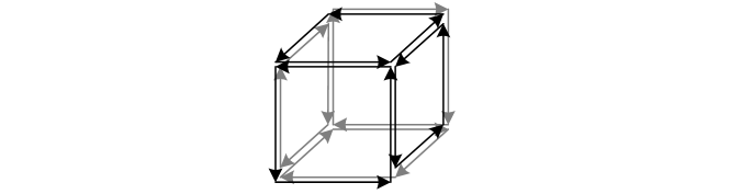
Figure C.8: The 3-form $\mathrm{d}\varphi=\mathrm{d}^{2}\psi$ sums $\psi$ over the edges of the faces of a cube. The sum vanishes since each edge is counted twice with opposite signs.

In a holonomic frame, we can obtain an expression for $\mathrm{d}\varphi$ in terms of coordinates

$$\mathrm{d}\varphi =\sum_{\mu_{0}<\dotsb<\mu_{k}}\left(\sum_{j=0}^{k}\left(-1\right)^{j}\frac{\partial}{\partial x^{\mu_{j}}}\varphi_{\mu_{0}\dots\mu_{j-1}\mu_{j+1}\dots\mu_{k}}\right)\mathrm{d}x^{\mu_{0}}\wedge\dotsb\wedge\mathrm{d}x^{\mu_{k}}$$ (C.16)

$$=\frac{\partial}{\partial x^{\mu_{0}}}\varphi_{\mu_{1}\dots\mu_{k}}\mathrm{d}x^{\mu_{0}}\wedge\dotsb\wedge\mathrm{d}x^{\mu_{k}}$$

$$=\frac{\partial\varphi_{I}}{\partial x^{\mu_{0}}}\mathrm{d}x^{\mu_{0}}\wedge\mathrm{d}x^{I},$$

so that in terms of array components we have

$$\left(\mathrm{d}\varphi\right)_{\mu_{0}\dots\mu_{k}} =\sum_{j=0}^{k}\left(-1\right)^{j}\frac{\partial}{\partial x^{\mu_{j}}}\varphi_{\mu_{0}\dots\mu_{j-1}\mu_{j+1}\dots\mu_{k}}.$$ (C.17)

It is not hard to see that the exterior derivative commutes with the pullback, i.e. $\Phi^{*}\mathrm{d}\varphi=\mathrm{d}\Phi^{*}\varphi$.

$\triangle$ Despite a convenient description using coordinates associated with a holonomic frame, it is important to keep in mind that the exterior derivative of a form is frame- and coordinate-independent.

If we include an inner product, vector calculus can be seen to correspond to exterior calculus on $\mathbb{R}^{3}$, and can thus be generalized to arbitrary dimensions:

• For a function (0-form) $f$, the components of the 1-form $\mathrm{d}f$ correspond to those of the gradient of $f$, i.e. $\left(\mathrm{d}f\right)_{\mu}=(\nabla f)^{\mu}$ or $\nabla f=(\mathrm{d}f)^{\sharp}$; a generalization of the gradient is then the 1-form $\mathrm{d}f$

• For a 1-form with components equal to those of a vector $\varphi_{\mu}=v^{\mu}$, the components of $\mathrm{d}\varphi$ correspond to those of the curl of $v$, i.e. $(\mathrm{d}\varphi)_{\mu}=(\nabla\times v)^{\mu}$ or $(\nabla\times v)=(*\mathrm{d}(v^{\flat}))^{\sharp}$; a generalization of the curl is then the 2-form $\mathrm{d}\varphi$

• For a 2-form with components equal to those of a vector $\psi_{\mu}=(*\varphi)_{\mu}=v^{\mu}$, the value of $\mathrm{d}\psi$ corresponds to the value of the divergence of $v$, i.e. $\mathrm{d}\psi=\nabla\cdot v$ or $\nabla\cdot v=*\mathrm{d}(*(v^{\flat}))$; a generalization of the divergence is then the value $*\mathrm{d}(*\varphi)$

In $\mathbb{R}^{3}$ the relations curl grad = div curl = 0 thus correspond to the property $\mathrm{d}^{2}=0$. Note that we have used the musical isomorphisms on $\mathbb{R}^{3}$, which imply an inner product, as does the Hodge star. The generalizations can be extended to a pseudo inner product with signature $\left(r,s\right)$ by defining the divergence as

$$\mathrm{div}\left(v\right)\equiv(-1)^{s}*\mathrm{d}(*v^{\flat}),$$ (C.18)

which is then independent of both signature and orientation.

Finally, the classical gradient, curl, and divergence integral theorems in vector calculus are generalized to Stokes’ theorem: for an $(n-1)$-form $\varphi$ on a compact oriented manifold $M^{n}$ with boundary $\partial M$,

$$\int_{M}\,\mathrm{d}\varphi=\int_{\partial M}\varphi.$$ (C.19)

This is essentially the integral form of the property $\mathrm{d}^{2}=0$: summing $\mathrm{d}\varphi$ over $M$ can be pictured as summing $\varphi$ over the boundaries of infinitesimal volumes, so that all internal boundaries cancel and what is left is $\varphi$ over the outer boundary $\partial M$.

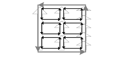
Figure C.9: The integral of $\mathrm{d}\varphi$ over $M$ can be pictured as summing $\varphi$ over the boundaries of infinitesimal volumes, so that all internal boundaries cancel and what is left is $\varphi$ over the outer boundary $\partial M$.

We will not address the details of defining integration on manifolds here, but the basic idea is relatively straightforward: a coordinate chart maps an $n$-dimensional sub-manifold $U$ of $M^{n}$ to $S\in\mathbb{R}^{n}$; an $n$-form $\varphi$ can then be written $f(x_{I})\,\mathrm{d}x^{I}$, and its integral over $U$ is defined to be $\int_{S}f(x_{I})\,\mathrm{d}x^{I}$, which can be shown to be coordinate-independent. Note that without additional structure on the manifold, we cannot integrate functions or other forms over $M^{n}$ besides $n$-forms (or pseudo $n$-forms if $U$ is non-orientable).

We can further generalize the divergence to $k$-forms $\varphi$ by defining the codifferential (AKA coderivative, exterior coderivative)

$$\begin{aligned} \delta\varphi&\equiv(-1)^{k}*^{-1}\mathrm{d}(*\varphi)\\ &=(-1)^{n(k+1)+s+1}*\mathrm{d}(*\varphi)\\ \Rightarrow\mathrm{div}\left(v\right)&=-\delta v^{\flat}.\end{aligned}$$ (C.20)

The map $\delta:\Lambda^{k}M\to\Lambda^{k-1}M$ does not follow the Leibniz rule and so is not a derivation. However, we do have $\delta^{2}=0$, so that we may write $\Delta\equiv\left(\mathrm{d}+\delta\right)^{2}=\mathrm{d}\delta+\delta\mathrm{d}$, which (usually for $s=0$) is called the Laplace-Beltrami operator (AKA Laplace operator, Laplacian, Laplace–de Rham operator); a form on a Riemannian manifold for which it vanishes is called a harmonic form. For $f\in\Lambda^{0}M$ we have $\delta f=0$ and $\Delta f=-\mathrm{div}\left(\nabla f\right)$; despite the sign, this last is often itself written $\Delta f\equiv\nabla^{2}f\equiv\nabla\cdot\nabla f$, except on a flat Lorentzian manifold where it is denoted $\square f=\partial^{\mu}\partial_{\mu}f\equiv-\partial_{t}^{2}f+\Delta f$, where $\square$ is called the d’Alembertian (AKA d’Alembert operator, wave operator, box operator), whose spatial part $\Delta$ is called the Laplacian (AKA Laplace operator). $\Delta f=0$ is then called Laplace’s equation, while a fixed $\rho\in\Lambda^{0}M$ defines Poisson’s equation $\Delta f=\rho$.

$\triangle$ In the mostly minuses signature on a Lorentzian manifold, the operators above may be defined with a negative sign. It is also important to remember that the sign of $\Delta$ may change depending upon whether it is applied to a function or a form.

If $\varphi\in\Lambda^{k}M$ and $\psi\in\Lambda^{k+1}M$ so that $\mathrm{d}\left(\varphi\wedge*\psi\right)\in\Lambda^{n}M$, it is not hard to see that

$$\int_{\partial M}\left(\varphi\wedge*\psi\right) =\int_{M}\left\langle\mathrm{d}\varphi,\psi\right\rangle\Omega-\left\langle\varphi,\delta\psi\right\rangle\Omega,$$ (C.21)

which means that if $\varphi\wedge*\psi$ vanishes on $\partial M$ (or $\partial M=0$) we have $\int_{M}\left\langle\mathrm{d}\varphi,\psi\right\rangle\Omega=\int_{M}\left\langle\varphi,\delta\psi\right\rangle\Omega$. In particular, for $f\in\Lambda^{0}M$ and $v^{\flat}\in\Lambda^{1}M$, we have

$$\int_{\partial M}f\left(*v^{\flat}\right) =\int_{M}\left\langle\nabla f,v\right\rangle\Omega+f\mathrm{div}\left(v\right)\Omega,$$ (C.22)

or for $f=1$ and recalling that $i_{v}\Omega=*(v^{\flat})$,

$$\int_{\partial M}*v^{\flat} =\int_{M}\mathrm{div}\left(v\right)\Omega$$ (C.23)

$$\Rightarrow\int_{M}\mathrm{div}\left(v\right)\Omega =\int_{\partial M}i_{v}\Omega$$ (C.24)

$$=\int_{\partial M}\left\langle v,\hat{n}\right\rangle i_{\hat{n}}\Omega,$$ (C.25)

where $\hat{n}$ is the unit normal vector to $\partial M$, the classical divergence theorem (AKA Gauss’s theorem, Ostrogradsky’s theorem).

C.6 Relationships between derivations

We can define one other derivation on $k$-forms, the interior derivative (AKA inner derivative, inner multiplication), which is the generalization of the interior product to forms on manifolds, i.e. for a given vector $v$ it is the graded degree $-1$ derivation

$$\left(i_{v}\varphi\right)\left(w_{2},\dotsc,w_{k}\right)\equiv\varphi\left(v,w_{2},\dotsc,w_{k}\right)$$ (C.26)

on $k$-forms $\varphi$, which follows the graded Leibniz rule

$$i_{v}\left(\varphi\wedge\psi\right)=(i_{v}\varphi)\wedge\psi+\left(-1\right)^{k}\varphi\wedge(i_{v}\psi).$$ (C.27)

The graded commutativity of forms immediately gives the property $i_{v}i_{w}+i_{w}i_{v}=i_{v}^{2}=0$. We define $i_{v}f\equiv 0$ for a 0-form $f$ and note that $i_{v}\Omega=*(v^{\flat})$.

The interior, exterior, and Lie derivatives then form an infinite-dimensional graded Lie algebra with the following relations:

• $\left[L_{v},L_{w}\right]\equiv L_{v}L_{w}-L_{w}L_{v}=L_{\left[v,w\right]}$

• $\left[i_{v},i_{w}\right]\equiv i_{v}i_{w}+i_{w}i_{v}=0$

• $\left[\mathrm{d},\mathrm{d}\right]\equiv\mathrm{d}^{2}+\mathrm{d}^{2}=0$

• $\left[L_{v},i_{w}\right]\equiv L_{v}i_{w}-i_{w}L_{v}=i_{\left[v,w\right]}$

• $\left[L_{v},\mathrm{d}\right]\equiv L_{v}\mathrm{d}-\mathrm{d}L_{v}=0$

• $\left[i_{v},\mathrm{d}\right]\equiv i_{v}\mathrm{d}+\mathrm{d}i_{v}=L_{v}$

This last relation is sometimes called Cartan’s formula (AKA Cartan’s magic formula).

Appendix D The divergence, currents, and tensor densities

D.1 Coordinate and tensor divergences

Using the results from Section 4.4, we can derive many useful coordinate dependent relations. Adopting the common abbreviation

$$\sqrt{g}\equiv\sqrt{\left|\det\left(g_{\mu\nu}\right)\right|}$$ (D.1)

and including torsion for completeness, we expand both sides of the coordinate divergence expression to get

$$\partial_{\lambda}\sqrt{g}=\sqrt{g}\left(?\Gamma^{\mu}{}_{\lambda\mu}?-?T^{\mu}{}_{\mu\lambda}?\right),$$ (D.2)

which along with the expressions for the metric derivative from Section 4.2 yields

$$\begin{aligned} \partial_{\lambda}\left(\sqrt{g}g^{\mu\nu}\right)&=\sqrt{g}\left(g^{\mu\nu}?\Gamma^{\sigma}{}_{\lambda\sigma}?-g^{\mu\nu}?T^{\sigma}{}_{\sigma\lambda}?-?\Gamma^{\mu\nu}{}_{\lambda}?-?\Gamma^{\nu\mu}{}_{\lambda}?\right)\\ \Rightarrow\partial_{\nu}\left(\sqrt{g}g^{\mu\nu}\right)&=-\sqrt{g}\left(?\Gamma^{\mu\nu}{}_{\nu}?-?T^{\nu\mu}{}_{\nu}?\right).\end{aligned}$$ (D.3)

From $\det\left(\exp\left(g\right)\right)=\exp\left(\mathrm{tr}\left(g\right)\right)\Rightarrow\ln\left(\det\left(g\right)\right)=\mathrm{tr}\left(\ln\left(g\right)\right)$, we can take the derivative of the components upon which it turns out that

$$\frac{1}{\det\left(g\right)}\partial_{\lambda}\left(\det\left(g\right)\right) =\mathrm{tr}\left(g^{-1}\partial_{\lambda}g\right)$$ (D.4)

$$=g^{\mu\nu}\partial_{\lambda}g_{\mu\nu}$$

$$\Rightarrow\partial_{\lambda}\sqrt{g} =\frac{1}{2}\sqrt{g}g^{\mu\nu}\partial_{\lambda}g_{\mu\nu}$$

$$\Rightarrow?\Gamma^{\mu}{}_{\lambda\mu}?-?T^{\mu}{}_{\mu\lambda}? =\frac{1}{2}g^{\mu\nu}\partial_{\lambda}g_{\mu\nu}.$$

By considering the inverse matrix, we see that these expressions are also valid with $g^{\mu\nu}\partial_{\lambda}g_{\mu\nu}\rightarrow-g_{\mu\nu}\partial_{\lambda}g^{\mu\nu}$. The first line above actually applies to any variation; applying it to the Lie derivative and using its coordinate expression gives us

$$\begin{aligned} L_{u}\sqrt{g}&=\sqrt{g}\mathrm{div}\left(u\right)\\ \Rightarrow\mathrm{div}\left(u\right)&=\frac{1}{2}g^{\mu\nu}L_{u}g_{\mu\nu}.\end{aligned}$$ (D.5)

If we consider an anti-symmetric tensor $F^{\mu\nu}$ and a symmetric tensor $G^{\mu\nu}$, it is not hard to see that

$$\begin{aligned} \nabla_{\nu}F^{\mu\nu}-?T^{\lambda}{}_{\lambda\nu}?F^{\mu\nu}&=\frac{1}{\sqrt{g}}\partial_{\nu}\left(\sqrt{g}F^{\mu\nu}\right)-\frac{1}{2}?T^{\mu}{}_{\lambda\nu}?F^{\lambda\nu},\\ \nabla_{\nu}G^{\mu\nu}-?T^{\lambda}{}_{\lambda\nu}?G^{\mu\nu}&=\frac{1}{\sqrt{g}}\partial_{\nu}\left(\sqrt{g}G^{\mu\nu}\right)+?\Gamma^{\mu}{}_{\lambda\nu}?G^{\lambda\nu},\\ \nabla_{\nu}?G_{\mu}{}^{\nu}?-?T^{\lambda}{}_{\lambda\nu}??G_{\mu}{}^{\nu}?&=\frac{1}{\sqrt{g}}\partial_{\nu}\left(\sqrt{g}?G_{\mu}{}^{\nu}?\right)-?\Gamma^{\lambda}{}_{\mu\nu}??G_{\lambda}{}^{\nu}?\\ &=\frac{1}{\sqrt{g}}\partial_{\nu}\left(\sqrt{g}?G_{\mu}{}^{\nu}?\right)-\frac{1}{2}\partial_{\mu}g_{\lambda\nu}G^{\lambda\nu}+?T^{\lambda}{}_{\mu\nu}??G_{\lambda}{}^{\nu}?.\end{aligned}$$ (D.6)

The above expressions are more commonly presented with zero torsion, under which condition we denote the covariant derivative $\overline{\nabla}_{\nu}$; this then defines the “divergence” of the tensor. It can also be shown ([2] p. 365) that the “divergence” of an exterior $k$-form expressed as an anti-symmetric tensor can be written in terms of the hodge star as

$$\begin{aligned} \overline{\nabla}^{\nu}F_{\nu\mu_{2}\cdots\mu_{k}}&\equiv g^{\nu\mu_{1}}\overline{\nabla}_{\nu}F_{\mu_{1}\cdots\mu_{k}}\\ &=-\left(\delta F\right)_{\mu_{2}\cdots\mu_{k}}\\ &=\left(-1\right){}^{n(k+1)+s}\left(*\mathrm{d}\left(*F\right)\right)_{\mu_{2}\cdots\mu_{k}}.\end{aligned}$$ (D.7)

D.2 Coordinate and tensor divergence theorems

The expression for the divergence theorem from Section 4.4 is

$$\int_{V}\mathrm{div}(u)\mathrm{d}V =\int_{\partial V}i_{u}\mathrm{d}V$$ (D.8)

$$=\int_{\partial V}\left\langle u,\hat{n}\right\rangle\mathrm{d}S,$$

where $V$ is an $n$-dimensional compact submanifold of $M^{n}$, $\hat{n}$ is the unit normal vector to $\partial V$, and $\mathrm{d}S\equiv i_{\hat{n}}\mathrm{d}V$ is the induced volume element (“surface element”) for $\partial V$. If we choose an orthonormal frame with $e_{1}=\hat{n}$ on $\partial V$, the divergence theorem can be written

$$\int_{V}\mathrm{div}(u)\mathrm{d}V =\int_{\partial V}u^{1}\mathrm{d}S,$$ (D.9)

and if we can choose coordinates with $x^{1}$ constant on $\partial V$ and normal to it, the divergence theorem can be written

$$\int_{V}\partial_{\lambda}\left(\sqrt{g}u^{\lambda}\right)\mathrm{d}^{n}x =\int_{\partial V}\sqrt{g}\mathrm{d}x^{1}\left(u\right)\mathrm{d}^{n-1}x$$ (D.10)

$$=\int_{\partial V}u^{1}\sqrt{g}\mathrm{d}^{n-1}x,$$

where $\mathrm{d}^{n}x\equiv\mathrm{d}x^{1}\wedge\cdots\wedge\mathrm{d}x^{n}$ and $\mathrm{d}^{n-1}x\equiv\mathrm{d}x^{2}\wedge\cdots\wedge\mathrm{d}x^{n}$.

Since the “divergence” of a tensor $T$ with order greater than 1 is tensor-valued, and the parallel transport of tensors is path-dependent, we cannot in general integrate to get a divergence theorem for tensors. In the case of a flat metric and zero torsion however, we can choose coordinates whose coordinate frame is orthonormal, so that the frame is its own parallel transport, i.e. $\nabla_{v}\left(\beta^{\mu}\right)=0$. For e.g. a tensor $T^{ab}$, we can then define a coordinate-dependent vector $J^{\mu}$ for each index $\mu$

$$J^{\mu} \equiv T\left(\beta^{\mu},\quad\right)$$ (D.11)

$$\Rightarrow\left(J^{\mu}\right)^{b} =T^{\mu b}$$

$$\Rightarrow\overline{\nabla}_{v}J^{\mu} \overset{\cancel{R}}{=}\beta^{\mu}\overline{\nabla}_{v}T$$

$$\Rightarrow\overline{\nabla}_{b}\left(J^{\mu}\right)^{b} \overset{\cancel{R}}{=}\overline{\nabla}_{b}T^{\mu b}$$

$$\Rightarrow\int_{V}\overline{\nabla}_{b}T^{\mu b}\mathrm{d}V \overset{\cancel{R}}{=}\int_{V}\overline{\nabla}_{b}\left(J^{\mu}\right)^{b}\mathrm{d}V$$

$$=\int_{\partial V}T^{\mu}{}_{b}\hat{n}^{b}\mathrm{d}S.$$

For arbitrary coordinates, the components of the coordinate frame are by definition constant, i.e. $\partial_{v}\left(\mathrm{d}x^{\mu}\right)=0$; we can therefore write

$$\sqrt{g}J^{\mu} \equiv\sqrt{g}T\left(\mathrm{d}x^{\mu},\quad\right)$$ (D.12)

$$\Rightarrow\partial_{\nu}\left(\sqrt{g}J^{\mu}\right)^{\nu} =\partial_{\nu}\left(\sqrt{g}T^{\mu\nu}\right)$$

$$\Rightarrow\int_{V}\partial_{\nu}\left(\sqrt{g}T^{\mu\nu}\right)\mathrm{d}^{n}x =\int_{V}\partial_{\nu}\left(\sqrt{g}J^{\mu}\right)^{\nu}\mathrm{d}^{n}x$$

$$=\int_{V}\nabla_{b}\left(J^{\mu}\right)^{b}\mathrm{d}V$$

$$=\int_{\partial V}T^{\mu}{}_{b}\hat{n}^{b}\mathrm{d}S.$$

This relation remains true in the presence of both curvature and torsion, however it is important to note that $\partial_{\nu}\left(\sqrt{g}T^{\mu\nu}\right)$ is not a “divergence” and $T^{\mu b}=\left(J^{\mu}\right)^{b}$ is coordinate-dependent. In the special case of an anti-symmetric tensor under zero torsion, we can write

$$\int_{V}\overline{\nabla}_{\nu}F^{\mu\nu}\mathrm{d}V =\int_{V}\partial_{\nu}\left(\sqrt{g}F^{\mu\nu}\right)\mathrm{d}^{n}x$$ (D.13)

$$=\int_{\partial V}F^{\mu}{}_{b}\hat{n}^{b}\mathrm{d}S.$$

D.3 Current forms and densities

In Section 4.4 we defined the current vector (AKA flux) $j\equiv\rho u$, where $\rho$ is the density of the physical quantity $Q$ and $u$ is a velocity field, and then combined them into the four-current $J\equiv(\rho,j^{\mu})$. There are a number quantities that can be defined around this concept:

Quantity	Definition	Meaning
Current vector	$j\equiv\rho u$	The vector whose length is the amount of $Q$ per unit time crossing a unit area perpendicular to $j$
Current form	$\begin{aligned} \zeta&\equiv i_{j}\mathrm{d}V\\ &=\left\langle j,\hat{n}\right\rangle\mathrm{d}S\end{aligned}$	The $(n-1)$-form which gives the amount of $Q$ per unit time crossing the area defined by the argument vectors
Current density	$\begin{aligned} \mathfrak{j}&\equiv\sqrt{g}\,j\\ \Rightarrow\zeta&=\mathfrak{j}^{1}\mathrm{d}^{2}x\end{aligned}$	The vector whose coordinate length is the amount of $Q$ per unit time crossing a unit coordinate area perpendicular to $j$
Current	$\begin{aligned} I_{S}&\equiv\int_{S}\zeta\\ &=\int_{S}\left\langle j,\hat{n}\right\rangle\mathrm{d}S\\ &=\int_{S}\mathfrak{j}^{1}\mathrm{d}^{2}x\end{aligned}$	The amount of $Q$ per unit time crossing $S$
Four-current	$J\equiv(\rho,j^{\mu})$	Current vector on the spacetime manifold

Table D.1: Quantities related to current.

Notes: $\rho$ is the density of the physical quantity $Q$, $u$ is a velocity field, $\hat{n}$ is the unit normal to a surface $S$, and $\mathrm{d}^{3}x$ are coordinates with $x^{1}$ constant on $S$ and normal to it. The four-current can be generalized to other Lorentzian manifolds, and can also be turned into a form $\xi\equiv i_{J}\mathrm{d}V$ or a density $\mathfrak{J}\equiv\sqrt{g}\,J$.

$\triangle$ Note that the terms flux and current (as well as flux density and current density) are not used consistently in the literature.

D.4 Tensor densities

The current density $\mathfrak{j}$ defined in the previous section is an example of a tensor density, which in general takes the form

$$\mathfrak{T}\equiv\sqrt{g}^{W}T,$$ (D.14)

where $T$ is a tensor and $W$ is called the weight. Note that tensor densities are not coordinate-independent quantities, and $\sqrt{g}$ itself can thus be called a scalar density.

From the expressions in the preceding sections we get

$$\partial_{\lambda}\left(\mathfrak{T}\right) =\sqrt{g}^{W}\partial_{\lambda}T+W\left(?\Gamma^{\mu}{}_{\lambda\mu}?-?T^{\mu}{}_{\mu\lambda}?\right)\mathfrak{T}$$ (D.15)

$$=\sqrt{g}^{W}\partial_{\lambda}T+\frac{W}{2}g^{\mu\nu}\partial_{\lambda}g_{\mu\nu}\mathfrak{T},$$

$$L_{u}\left(\mathfrak{T}\right) =\sqrt{g}^{W}L_{u}T+W\mathrm{div}\left(u\right)\mathfrak{T}$$

$$=\sqrt{g}^{W}L_{u}T+\frac{W}{2}g^{\mu\nu}L_{u}g_{\mu\nu}\mathfrak{T},$$

$$\nabla_{\lambda}\left(\mathfrak{T}\right) =\sqrt{g}^{W}\nabla_{\lambda}T,$$

where the last is due to the covariant derivative of the metric vanishing. In particular, this means that for zero torsion the divergence of a vector density is

$$\overline{\nabla}_{\lambda}\mathfrak{J}^{\lambda} =\sqrt{g}\overline{\nabla}_{\lambda}J^{\lambda}$$ (D.16)

$$=\sqrt{g}\mathrm{div}\left(J\right)$$

$$=\partial_{\lambda}\mathfrak{J}^{\lambda}.$$

$\triangle$ A potential source of confusion is the use of the word “density” to indicate both an amount per unit area or volume and the presence of the coordinate-dependent factor $\sqrt{g}$, which as in the current density typically reflects the volume in question being a unit coordinate volume instead of metric volume.

D.5 Conserved currents and quantities

In Section 4.4 we saw that a Lorentzian conserved current $\mathrm{div}(J)=0$ does not imply a conserved quantity in the presence of curvature. If we are willing to consider coordinate-dependent currents, at any given point we can choose Riemann normal coordinates, which allows us to recover a conserved quantity at that point in those coordinates.

In the integral form, we may also identify a coordinate-dependent conserved quantity for a Lorentzian conserved current by integrating over a space-like volume $S$ with coordinates such that $t\equiv x^{0}$ is constant on $S$ and normal to it, while $x^{1}$ is constant on $\partial S$ and normal to it:

$$0 =\int_{S}\sqrt{g}\mathrm{div}(J)\mathrm{d}^{3}x$$ (D.17)

$$=\int_{S}\partial_{\mu}\mathfrak{J}^{\mu}\mathrm{d}^{3}x$$

$$=\partial_{t}\left(\int_{S}\mathfrak{J}^{t}\mathrm{d}^{3}x\right)+\int_{S}\partial_{i}\mathfrak{J}^{i}\mathrm{d}^{3}x$$

$$=\partial_{t}\left(\int_{S}\mathfrak{J}^{t}\mathrm{d}^{3}x\right)+\int_{\partial S}\mathfrak{J}^{1}\mathrm{d}^{2}x$$

Note that the coordinate-dependent factor $\sqrt{g}$ in $\mathfrak{J}=\sqrt{g}J$ cannot be absorbed into either $\mathrm{d}^{3}x$ or $\mathrm{d}^{2}x$ to yield a coordinate-independent quantity. More specifically, if $\mathfrak{J}$ is either also normal to $S$ or vanishes on $\partial S$, we have $\partial_{t}\left(\int_{S}\mathfrak{J}^{t}\mathrm{d}^{3}x\right)=0$. This also holds if $S$ is infinite and $\mathfrak{J}$ vanishes rapidly enough at spatial infinity.

$\triangle$ A conserved quantity as we have defined it is a quantity whose amount in a volume of space changes in time by the net amount that crosses the volume boundary. This concept is not valid when $\mathrm{div}(J)=0$ in the presence of spacetime curvature, but it is important to remember that this still means that $\int_{\partial V}\left\langle J,\hat{n}\right\rangle\mathrm{d}S=0$, so that the same amount of the quantity enters and exits any finite volume of spacetime; it is in this sense that the current is “conserved.”

With regard to tensors, we can conclude from the divergence theorem variants in Section D.2 that in the case of an orthonormal coordinate frame under a flat metric and the Levi-Civita covariant derivative, we have a coordinate-dependent conserved quantity for each component of a tensor, corresponding to a coordinate-dependent conserved current:

$$\overline{\nabla}_{\nu}T^{\mu\nu} =0$$ (D.18)

$$\Rightarrow\partial_{0}T^{\mu 0} \overset{\cancel{R}}{=}-\overline{\nabla}_{j}T^{\mu j},$$

$$\int_{\partial V}T^{\mu}{}_{b}\hat{n}^{b}\mathrm{d}S \overset{\cancel{R}}{=}0$$

In the special case of an anti-symmetric tensor and the Levi-Civita covariant derivative we also have a divergence theorem, and therefore a coordinate-dependent conserved current for each component:

$$\overline{\nabla}_{\nu}F^{\mu\nu} =0$$ (D.19)

$$\Rightarrow\int_{\partial V}F^{\mu}{}_{b}\hat{n}^{b}\mathrm{d}S =0$$

References

- [1] M. do Carmo, Riemannian Geometry (Birkhäuser Boston, 1992)
- [2] T. Frankel, The Geometry of Physics (Cambridge University Press, 1997)
- [3] T. Frankel, Gravitational Curvature (W H Freeman and Company, 1979)
- [4] M. Göckeler and T. Schücker, Differential Geometry, Gauge Theories, and Gravity (Cambridge University Press, 1987)
- [5] A. Gray, “The volume of a small geodesic ball of a Riemannian manifold,” The Michigan Mathematical Journal 20 (1974), no. 4, 329-344, http://projecteuclid.org/euclid.mmj/1029001150
- [6] S. Kobayashi and K. Nomizu, Foundations of Differential Geometry (John Wiley & Sons, 1963)
- [7] C. Misner, K. Thorne and J. Wheeler, Gravitation (W H Freeman and Company, 1973)
- [8] P. Petersen, Riemannian Geometry (Springer, 2006)
- [9] R. Wald, General Relativity (University of Chicago Press, 1984)