Radiometric Measurements of Electron Temperature and Opacity of Ionospheric Perturbations

Abstract

Changes in the sky noise spectrum are used to characterize perturbations in the ionosphere. Observations were made at the same sidereal time on multiple days using a calibrated broadband dipole and radio spectrometer covering 80 to 185 MHz. In this frequency range, an ionospheric opacity perturbation changes both the electron thermal emission from the ionosphere and the absorption of the sky noise background. For the first time, these changes are confirmed to have the expected spectral signature and are used to derive the opacity and electron temperature associated with the perturbations as a function of local time. The observations were acquired at the Murchison Radio-astronomy Observatory in Western Australia from 18 April 2014 to 6 May 2014. They show perturbations that increase at sunrise, continue during the day, and decline after sunset. Magnitudes corresponding to an opacity of about 1 percent at 150 MHz with a typical electron temperature of about 800 K, were measured for the strongest perturbations.

Gindraft=false ROGERS ET AL. MEASUREMENTS OF ELECTRON TEMPERATURE Corresponding author: A. E. E. Rogers, M.I.T. Haystack Observatory off route 40, Westford, Massachusetts 01886 USA. (arogers@haystack.mit.edu)

1 Introduction

The ionospheric effects on radio propagation, which are fairly small in the VHF frequency band during normal ionospheric conditions, are still significant enough that they need to be taken into account for a ground based measurement of the signature of the epoch of reionization (EoR) [Bowman and Rogers, 2010]. An overview of these ionospheric chromatic effects is given by Vedantham et. al, [2010].

In this study, observational results of ionospheric effects in the 80-185 MHz frequency range are presented, including the first spectrometric detection of ionospheric radio emission, allowing the measurement of electron temperature in addition to ionospheric absorption. Understanding and being able to measure these effects is not only important for future measurements of the spectral signature of the EoR signature, but could also have applications in ionospheric remote sensing. Currently electron temperatures in the ionosphere can be measured either using incoherent scatter radars, or satellite-borne in situ measurements with Langmuir probes.

A riometer [Little and Leinbach, 1959] is an instrument that is used to measure ionospheric absorption. This instrument uses an antenna and a stable radio frontend to measure cosmic radio noise to infer the amount of absorption occurring in the ionosphere. The noise temperature measured by the instrument is equal to the sky noise brightness convolved with the antenna beam. This is a repeatable function of sidereal time if the variable effects of solar radiation, ionospheric absorption, and ionospheric emission are excluded. At frequencies below about 100 MHz, ionospheric absorption dominates. In this case observations of a decrease of the noise power from the maximum sky noise observed at that sidereal time can be used to measure the ionospheric absorption. The ”reference” curve of maximum power as a function of sidereal time can be measured at the night when the ionosphere is at minimum and the radio noise from the Sun is excluded. The receiver used in a riometer needs to be very stable in time, although accurate absolute calibration is not required.

While typically a riometer uses only a single frequency, the measurements reported in this paper were made with a wideband instrument and cover 80 to 185 MHz. This instrument was designed as part of the Experiment to Detect the Global EoR Signature (EDGES) for astronomical observations of the early universe [Bowman and Rogers, 2010; Bowman et al., 2008; Rogers and Bowman, 2008]. Like a riometer, it is very stable and repeatable in time. Further, its frequency response is very well calibrated (see Rogers and Bowman [2012] for details of the calibration method and the instrument) so that observed changes in the spectrum taken at the same time on successive days can be used to measure changes in ionospheric emission as well as absorption.

Observations reported here, which were made using the EDGES instrument deployed at the Murchison Radio-astronomy Observatory (MRO) at $(-26.7^{\circ}N~{},~{}116.6^{\circ}E)$ in Western Australia from 18 April 2014 to 6 May 2014, may not be the first radiometric measurements of the electron temperature in the ionosphere. Pawsey et al. [1951] report emission temperatures in the range 240 to 290 K at 1.6 and 2.0 MHz which could have been from the lower ionosphere. However, while at these low frequencies the emission from sky is completely reflected back into space during daytime, thermal emission from the earth can be propagated via a ground wave or be reflected from the ionosphere and atmospherics from lightning as well as man-made radio frequency interference (RFI). This makes observations at these low frequencies very difficult. A broadband spectrometer, such as the EDGES instrument, has the advantage over a traditional riometer that contaminating changes in the observed sky power due to solar emission, RFI, and the effects of severe weather conditions can be distinguished based on their spectral properties from the absorption and emission due to the ionosphere.

We describe our analysis method in Section 2. In Section 3, we present the data and principal results of the analysis, followed by interpretation and discussion in Section 4 and concluding remarks in Section 5.

2 Method

The noise power temperature from an antenna at a given frequency is equal to the sky noise brightness, $T_{sky}(\vec{\theta},\nu,t)$, convolved with the antenna beam directivity, $D(\vec{\theta},\nu)$,

$$T_{ant}(\nu,t)=T_{sky}(\vec{\theta},\nu,t)\otimes D(\vec{\theta},\nu)$$ (1)

where $\vec{\theta}$ is sky coordinate, $\nu$ is frequency, and $t$ is time [Rogers et al., 2004]. In the absence of the ionosphere, RFI and solar flares the spectrum, $T_{ant}(\nu)$, is a highly repeatable function of sidereal time. Its spectral shape follows the beam averaged power law of the sky brightness provided the beam shape is constant with frequency.

2.1 Ionosphere model

If an opacity change occurs in a region of uniform electron temperature, the change in the spectrum from the theory of radiative transfer [Chandrasekhar, 1960] is approximately

$$(-T_{B}f^{-s}+T_{e})f^{-2}\Delta\tau$$ (2)

where $T_{B}$ is $T_{ant}$ evaluated at 150 MHz, $T_{e}$ is the electron temperature of the perturbed region, $f$ is the normalized frequency given by $\nu/(150$ MHz), $\Delta\tau$ is the change in opacity at 150 MHz, and $s$ is the spectral index of the sky brightness power law spectrum.

This approximation is valid for the small opacity and small changes in the ionosphere expected in the frequency range 80 to 185 MHz. The spectral index is approximately 2.5 in this frequency range [Rogers and Bowman, 2008]. Typical attenuation through the ionosphere at 150 MHz is 0.015 dB at night and 0.1 dB during the day and is inversely proportional to frequency squared (Evans and Hagfors, 1968 and references therein).

2.2 Analysis

Two methods are used to analyze difference spectra for electron temperature and change in opacity. In the first method the average and standard deviation of the weighted electron temperature and average magnitude of the perturbations can be estimated from the difference spectra taken at the same sidereal time on different days. If there are $N$ days of data there will be $N(N-1)/2$ difference spectra that can be analyzed. Each difference spectrum is fitted to the function

$$af^{-2-s}+bf^{-2}$$ (3)

using weighted least squares. The perturbation in opacity and associated electron temperature are then derived from the best fit parameters $a$ and $b$, resulting in

$$\Delta\tau=-aT_{B}^{-1}$$ (4)

and

$$T_{e}=-(b/a)T_{B}.$$ (5)

In order to improve the detection and measurement of weak perturbations, their average magnitude and associated electron temperature can be estimated by conducting incoherent averaging of the coefficients derived from the difference spectra. Squaring equation (4) and multiplying equation (5) by $a$ eliminates the division by $a$ in equation (5) which results in

$$(\Delta\tau)^{2}=a^{2}T_{B}^{-2}$$ (6)

and

$$T_{e}=-abT_{B}/a^{2}.$$ (7)

The bias in $a^{2}$ and $ab$ due to Gaussian noise in the spectra can be removed by subtracting the noise expected in the absence of perturbations,

$$\overline{a^{2}}=\ \langle a^{2}\ -C_{aa}\ \mathrm{rms}^{2}\rangle$$ (8)

and

$$\overline{ab}=\ \langle ab\ -C_{ab}\ \mathrm{rms}^{2}\rangle$$ (9)

where $C_{aa}$ and $C_{ab}$ are the values from the covariance matrix used to fit each difference spectrum and $\mathrm{rms}$ is the root mean square (RMS) residual from the fit used to obtain the values of $a$ and $b$. This method is similar to the method of bias removal used for the incoherent averaging of interferometer correlation amplitudes [Rogers, Doeleman and Moran, 1995].

A sequence of 16 days of data from day 108 to 126 (excluding days 109, 115, 125) was analyzed in half hour integrations at the same sidereal time each day. The 16 days provide up to 120 difference spectra. A weighted average of the noise-corrected values of $\overline{a^{2}}$ and $\overline{ab}$ is made to improve the signal-to-noise ratio (SNR) of the measurement of the magnitude of opacity changes and the associated electron temperature. The average magnitude of the perturbations is computed using

$$\langle|\Delta\tau|\rangle\ =\Big{[}\sum\limits_{i=0}^{M-1}(\overline{{a_{i}}^{2}}T_{B}^{-2})\ /M\Big{]}^{1/2}$$ (10)

and the weighted average electron temperature is computed using

$$\langle T_{e}\rangle\ =-\sum\limits_{i=0}^{M-1}\overline{ab_{i}}T_{B}\ /\sum\limits_{i=0}^{M-1}\overline{{a_{i}}^{2}}$$ (11)

This averaging improves the SNR by approximately $2^{1/2}M^{1/4}$, where $M$ is the number of difference spectra used in equations (10) and (11).

The second method is to take the difference between the spectrum on a given day from the average of the spectra on all the other days at the same sidereal time. In this case the change in opacity and electron temperature are calculated from equations (4) and (5) and errors in these quantities can be estimated from the covariance matrix and the RMS residuals to the weighted least squares fit of the difference spectrum to function (3). The optimal weighting is equal to $1/\sigma^{2}$ where $\sigma$ is the expected noise as a function of frequency.

3 Results

Figures 1 and 2 show the magnitude of the perturbations and the associated electron temperature derived by the first method. The error bars in these figures are computed from the weighted RMS deviation of the noise-corrected values of $\Delta\tau$ and $T_{e}$ obtained from equations (6) and (7) from the mean values derived from equations (10) and (11), divided by $2^{1/2}M^{1/4}$. The incoherent averaging of results from many difference spectra is needed to obtain a sufficient SNR for measurements of the electron temperature during the night.

Examples of these differences for large perturbations are shown in Figure 3 along with the least squares fit to these spectra and the corresponding values of $\Delta\tau$ and electron temperature derived from equation (4) and (5). In this case the SNR for a single difference spectrum is sufficient to obtain the electron temperature with the errors from the least squares analysis of each spectrum.

The second method allows the variation in ionospheric opacity to be shown as a function of time for each day as shown in Figure 4. In this plot only the points with a good fit to the ionosphere are plotted. The missing points correspond to data corrupted by solar emission, RFI, or rain. Each point is from a 15 minute integration from independent data. The high correlation between adjacent points shows that, in most cases, the time scale for opacity changes in the ionosphere is longer than 15 minutes and on average is about an hour.

4 Discussion

The variation of opacity shown in Figure 1 is similar to the variations in the radiometric measurements of Steiger and Warwick [1961] at 18 MHz, who show a plot of attenuation vs local time on 16 December 1958. Their plot shows variations of ionospheric attenuation of about 2 dB, which corresponds to 0.7% at 150 MHz, on what they call a ”typical day”. The plot also shows the attenuation rising sharply at 6 hours local time and declining at 21 hours in a manner similar to that shown in Figure 1. The time scale for the variations is about one hour, consistent with those of Figure 4.

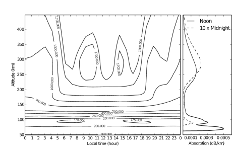
Figure 5: Electron temperature and absorption obtained from the IRI ($>$120 km) and MSIS ($<$120 km) models on on 2014-04-20 for the MRO at $(-26.7^{\circ}N,116.6^{\circ}E)$

The measurements of electron temperature shown in Figure 2 indicate that absorption is occurring at a broad range of altitudes. Figure 5 shows electron temperatures on 2014-04-20 at MRO based on the MSISE-90 model of Hedin [1991] and the IRI 2007 model of Bilitza and Reinisch [2008]. This indicates that the measured electron temperatures during the day time are comparable with model-based F-region electron temperatures.

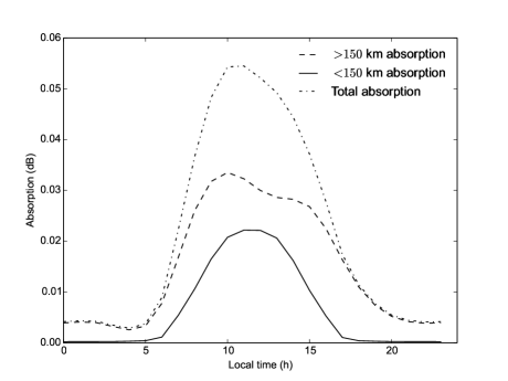
Figure 6: Modeled absorption based on electron densities from the IRI-2007 model, and collision frequencies based on Aggarwal et.al. [1979]. The model shows that during normal quiet geophysical conditions with normal D-region electron density, the F-region has significant absorption.

Figure 6 shows absorption of a single 150 MHz ray at 45^∘ zenith angle. This also supports the conclusion that slightly over half of the absorption occurs at altitudes over 150 km. The shape of the total absorption also agrees relatively well with Figure 1, which is reasonable, assuming that variation of opacity is to first order proportional to opacity. The absorption was computed using a variant of the Appleton-Lassen equation that ignores the magnetic field [Hargreaves, 1969]

$$A=4.6\cdot 10^{-5}\int\frac{N_{e}(h)\nu_{e}(h)}{\nu_{e}(h)^{2}+\omega^{2}}dh,$$ (12)

where $A$ is the attenuation in dB, $N_{e}(h)$ is altitude dependent electron density and $\omega^{2}$ is the angular frequency of the radio wave. Here, $\nu_{e}(h)$ is the electron collision frequency, including not only electron-neutral, but also electron-ion collisions, which are important in the F-region [Mitra and Shain, 1953]. The electron collision frequency height distribution $\nu_{e}=\langle\nu_{\mathrm{ei}}\rangle+\langle\nu_{\mathrm{en}}\rangle$ function shown in Figure 7 of Aggarwal et.al., [1979] was used to derive the attenuation curves plotted in Figure 6.

4.1 Extended Ionosphere model

The simple model of a single layer, considered in Section 2.1 can be extended to include many layers. In this case, if the modeled absorption is small, the spectrum of a ray after passage through layers on the ionosphere, $T(f)$, can be written as,

$$T(f)=T_{B}f^{-s}-T_{B}f^{-s}f^{-2}\sum_{r}L_{r}+f^{-2}\sum_{r}L_{r}T_{e}(r),$$ (13)

where $L_{r}$ is the absorption coefficient for a narrow altitude range interval at range $r$, $T_{B}f^{-s}$, is the spectrum of sky noise above the ionosphere in the direction from which the ray originates and $T_{e}(r)$ is electron temperature at range $r$. The sum is formed across the range of all layers though which the ray propagates. This ignores the change in sky noise spectrum through the ionosphere owing to the small losses involved.

For spectra $T(f)$ and $T^{\prime}(f)$ taken on different days at the same sidereal time, the difference spectrum, $\Delta T(f)$, is given by

$$\Delta T(f)=(-T_{B}f^{-s}f^{-2})\sum_{r}(L_{r}-L_{r}^{\prime})$$

$$+f^{-2}\sum_{r}(L_{r}T_{e}(r)-L^{\prime}_{r}T^{\prime}_{e}(r)).$$ (14)

Here the primed variables correspond to changed quantities in the spectrum $T^{\prime}(f)$. If the temperatures on the two different days are assumed equal $\tilde{T}_{e}=\tilde{T}^{\prime}_{e}$, then equation (14) can be simplified to

$$\Delta T(f)=(-T_{B}f^{-s}f^{-2}+f^{-2}\tilde{T}_{e})\Delta\tau,$$ (15)

In this case for a single ray path

$$\tilde{T}_{e}=\left(\sum_{r}L_{r}-L^{\prime}_{r}\right)^{-1}\sum_{r}(L_{r}-L^{\prime}_{r})T_{e}(r)$$ (16)

and

$$\Delta\tau=\sum_{r}L_{r}-L^{\prime}_{r}$$ (17)

If the day to day perturbations in the F-region dominate, the electron temperature derived from the difference spectrum would be an estimate of the electron temperature in the F-region. Conversely, if the perturbations in the D-region dominate, the electron temperature derived from the difference spectrum would be an estimate of the D-region temperature.

As we currently do not have a way to model the day-to-day variation in absorption, we have attempted to model the observed electron temperatures using the approximation that assumes there is a constant fractional change from day to day in attenuation for each layer, i.e., $L_{r}-L^{\prime}_{r}=cL_{r}$, where $c$ is an arbitrary constant. In this case, the measured electron temperature is the weighted average of electron temperature, weighted with attenuation in each layer. This simplified model, computed for a single $45^{\circ}$ slanted ray going through the ionosphere is shown in Figure 2, overlayed on the measurements. We used values of $N_{e}(r)$ and $T_{e}(r)$ obtained for the MRO location from the IRI-2007 and MSISE-90 models for our computations.

A more complete modeling of the electron temperature from the difference spectra requires estimates of changes in loss for each layer of the ray path, horizontal structure, refraction, as well as convolution over all the ray paths with the beam of the dipole antenna used for the measurements.

While the measurements of electron temperature agree reasonably well with this model during the daytime, the night temperatures are consistently lower in the measurements. The reason for this is unknown, but it could be caused by the model underestimating the D-region electron density or overestimating the F-region electron density during the night.

This study shows a novel method for measuring the electron temperature using a relatively inexpensive passive ground based radio remote sensing method. At present the instrument can only measure the electron temperature of changes in the ionosphere so the results presented here are weighted by the perturbations in the attenuation through the ionosphere. As data is acquired over a full year it will be possible to obtain the electron temperature weighted by the attenuation relative the minimum values observed at each sidereal time but it will require models or data from other instruments to obtain the electron temperature as a function of altitude.

5 Conclusions

The use of a well calibrated broadband spectrometer in the frequency range 80 to 185 MHz allows the radiometric measurement of the electron temperature of ionospheric perturbations in addition to the measurement of the attenuation changes through the ionosphere. The measurements agree relatively well with theory and previously published measurements.

Figure 1: Average magnitude of ionospheric perturbations, $\langle|\Delta\tau|\rangle$, vs local time over the 16 days from 18 April to 6 May 2014. Sunrise and sunset at ground level were at about 6.5 and 17.5 hours localtime respectively. The error bars are $\pm 1\sigma$

Figure 2: Circles represent average electron temperature of the region in which perturbations of ionospheric opacity occur vs local time. The error bars are $\pm 1\sigma$. The electron temperature was not well determined around 5 hours local time because of a combination of small perturbations and large sky noise from the transit of the galactic center at this time. The solid line represents the weighted sum of electron temperatures obtained from the IRI and MSIS model. The sum is weighted with absorption across altitudes 60 and 400 km.

Figure 3: Examples of the difference spectrum of the largest ionospheric perturbations at the Galactic hour angle of 14 hours which corresponds to a local time of about 17.75 hours. The dates of the 2 spectra whose difference was taken are given on the right of the plot along with the change in opacity at 150 MHz in units of parts per thousand and the associated electron temperature and $1~{}\sigma$ error from the best fit to the difference spectrum. An integration of 60 minutes was used with a small amount of data excluded due to RFI. The spectra are offset vertically for clarity.

Figure 4: Plots of the change of opacity vs local time for each day obtained from the difference between the spectrum taken at that local local time an the average spectrum for all days taken at the same sidereal time. The integration time was 15 minutes with some data excluded owing to RFI and weather conditions.

- [1]
- [Aggarwal, K. M., Nath, N., and Setty, C. S. G. K. (1979)] Aggarwal, K. M., Nath, N., and Setty, C. S. G. K. (1979). Collision frequency and transport properties of electrons in the ionosphere, Planetary and Space Science, 27, no. 6, 753-768.
- [Bilitza D., and Reinisch, B. (2008)] Bilitza D., and Reinisch, B. (2008), International Reference Ionosphere 2007: Improvements and new parameters, J. Adv. Space Res., 42, no. 4, 599-609.
- [Bowman, J. D., and Rogers A. E. E. (2010)] Bowman, J. D., and Rogers, A. E. E. (2010), A lower limit of for the duration of the reionization epoch, Nature, 468, no. 7325, 796-798.
- [Bowman J. D., Rogers, A. E. E., and Hewitt, J. N. (2008)] Bowman, J. D., Rogers, A. E. E., and Hewitt, J. N. (2008), Toward Empirical Constraints on the Global Redshifted 21 cm Brightness Temperature During the Epoch of Reionization, The Astrophysical Journal,, 676, 1.
- [Chandrasekhar(1960)] Chandrasekhar, S. (1960). Radiative transfer, Courier Dover Publications.
- [Dalgarno et al.(1967)] Dalgarno, A., Mo Bo McElroy, and Jo CG Walker (1967), The diurnal variation of ionospheric temperatures, Planetary and Space Science 15, no. 2, 331-345.
- [Evans, John V., and Tor Hagfors(1968)] Evans, John V., and Tor Hagfors (1968). Radar astronomy. New York: McGraw-Hill.
- [Hargreaves, J. K.(1969)] Hargreaves, J. K., (1969), Auroral absorption of HF radio waves in the ionosphere: A review of results from the first decade of riometry, Proceedings of the IEEE, 57, no. 8, 1348-1373.
- [Hedin, A. E.(1991)] Hedin, A. E., (1991), Extension of the MSIS Thermospheric Model into the Middle and Lower Atmosphere, J. Geophys. Res., 96, no. 1159.
- [Little and Leinbach (1959)] Little, Charles Gordon, and H. Leinbach (1959), The riometer-a device for the continuous measurement of ionospheric absorption, Proceedings of the IRE 47, no. 2, 315-320.
- [Mitra, A. P., and Shain, C. A. (1953)] Mitra, A. P., and Shain, C. A., (1953), The measurement of ionospheric absorption using observations of 18.3 Mc/s cosmic radio noise, Journal of Atmospheric and Terrestrial Physics, 4 no. 4, 204-218.
- [Pawsey, J. L., McCready L. L., and Gardner F. F. (1951)] Pawsey, J. L., McCready L. L., and Gardner F. F., (1951), Ionospheric thermal radiation at radio frequencies, Journal of Atmospheric and Terrestrial Physics, 1 no. 5, 261-277.
- [Rogers et al.(2004)] Rogers, Alan E E, Preethi Pratap, Eric Kratzenberg, and Marcos A. Diaz (2004), Calibration of active antenna arrays using a sky brightness model, Radio Science, 39, no. 2.
- [Rogers, A. E. E. and Bowman, J. D. (2008)] Rogers, A. E. E. and Bowman, J. D. (2008), Spectral Index of the Diffuse Radio Background Measured from 100 to 200 MHz, The Astronomical Journal, 136, 641.
- [Rogers, A. E., and Bowman, J. D. (2012)] Rogers, A. E., and Bowman, J. D. (2012), Absolute calibration of a wideband antenna and spectrometer for accurate sky noise temperature measurements, Radio Science, 47(6), doi:10.1029/2011RS004962.
- [Rogers, A. E. E., Doeleman, S. S., and Moran, J. M. (1995)] Rogers, A. E. E., Doeleman, S. S., and Moran, J. M. (1995), Fringe detection methods for very long baseline arrays, A.J., 109, 1391-1401.
- [Steiger, Walter R., and James W. Warwick (1961)] Steiger, Walter R., and James W. Warwick (1961), Observations of cosmic radio noise at 18 Mc/s in Hawaii, Journal of Geophysical Research, 66, no. 1, 57-66.
- [Vedantham, H. K., L. V. E. Koopmans, A. G. de Bruyn, S. J. Wijnholds, B. Ciardi, and M. A. Brentjens. (2013)] Vedantham, H. K., L. V. E. Koopmans, A. G. de Bruyn, S. J. Wijnholds, B. Ciardi, and M. A. Brentjens., (2013). Chromatic effects in the 21 cm global signal from the cosmic dawn, Monthly Notices of the Royal Astronomical Society, stt1878.