Turbulent General Magnetic Reconnection

Abstract

Plasma flows with an MHD-like turbulent inertial range, such as the solar wind, vitiate many assumptions of standard theories of magnetic reconnection. In particular, the “roughness” of turbulent velocity and magnetic fields implies that magnetic field-lines are nowhere “frozen-in” in the usual sense. This situation demands an essential generalization of the so-called “General Magnetic Reconnection” (GMR) theory. Following ideas of Axford and Lazarian & Vishniac, we identify magnetic field-lines by “tagging” them with plasma fluid elements and then determine their slip-velocity relative to the plasma fluid by integrating in arc-length along the wandering field-lines. The main new concept introduced here is the slip-velocity source vector, which gives the rate of development of slip-velocity per unit arc-length of field line. The slip-source vector is the ratio of the curl of the non-ideal electric field R in the Generalized Ohm’s Law and the magnetic field strength. It diverges at magnetic nulls, unifying GMR with theories of magnetic null-point reconnection. Only under restrictive assumptions is the slip-velocity related to the gradient of the line-voltage or “quasi-potential” obtained by integrating the parallel electric field $R_{\|}$ along field-lines. In an MHD turbulent inertial-range ${\mathit{\nabla}}$$\times$R becomes extremely large while $R_{\|}$ is tiny, so that line-slippage occurs freely even as a description by ideal MHD becomes accurate. This “paradox” is resolved by the understanding that ideal MHD is valid for a turbulent inertial-range not in the standard sense but in a “weak” sense which does not imply magnetic line-freezing. The mathematical notion of “weak solution” is here explained in physical terms of spatial coarse-graining and renormalization-group (RG) theory. We give a new first-principles argument for the “weak” validity of the ideal Ohm’s law in the inertial range, via rigorous estimates of the terms in the Generalized Ohm’s Law for an electron-ion plasma. Particular attention is paid to the conditions in the solar wind, a collisionless, magnetized plasma. Coarse-grained to inertial-range lengths, all of the non-ideal terms (from collisional resistivity, Hall field, electron pressure anisotropy, and electron inertia) are shown to be irrelevant in the RG sense and large-scale reconnection is thus governed solely by ideal dynamics. We briefly discuss some implications for heliospheric reconnection, in particular for deviations from the Parker spiral model of interplanetary magnetic field. Solar wind observations show that reconnection in a turbulence-broadened heliospheric current sheet, consistent with the Lazarian & Vishniac (1999) theory, leads to slip velocities that cause field-lines to lag relative to the spiral model.

1 Introduction

A fundamental assumption of most current theories of magnetic reconnection is that ideal line-freezing holds to very good approximation for most of space, except within narrow, sparsely distributed current layers. This includes the elegant mathematical theories which propose a key role for field-parallel electric fields (Schindler et al., 1988; Hesse & Schindler, 1988), magnetic flipping (Priest & Forbes, 1992), quasi-separatrix layers (Priest & Démoulin, 1995), and multi-valued flux-tube velocities (Priest et al., 2003). More precisely, most current theories assume that in the generalized Ohm’s law

$${\textit{{E}}}+{\textit{{u}}}\hbox{\boldmath$\times$}{\textit{{B}}}={\textit{{R}}},$$ (1.1)

the non-ideal electric field R is large in isolated spatial regions of small total volume and that outside these “diffusion regions” where reconnection solely occurs, ideal MHD equations are valid and magnetic field-lines are “frozen-in” to a good approximation. One thus finds statements in the literature such as “reconnection occurs when there is a breakdown of ideal MHD and therefore an electric field component ($E_{\|}$) along the magnetic field…” (Priest & Démoulin, 1995). Such concepts are motivated especially by the conditions of an initially quiet solar corona, where the underlying assumption of well-localized regions of flux-freezing violation may be a good approximation in the early stages of coronal reconnection.

The basic assumptions of the standard reconnection theories are, however, badly violated in plasmas with a turbulent range governed by MHD-like dynamics, such as the solar wind at distances from the sun ranging from 0.1 to 100 AU. Here non-ideal electric fields R are very small in r.m.s. magnitude, ideal Ohm’s law is valid down to very small scales within the “inertial range” , and yet magnetic field-lines are not well “frozen-in” anywhere in space (see Burlaga et al. (1982); Khabarova & Obridko (2012); Richardson et al. (2013) and section 5 for more discussion). The failure of standard flux-freezing in turbulent MHD in the ideal limit (“high magnetic Reynolds-number”) has been understood previously from several points of view. A spatial coarse-graining approach similar in spirit to renormalization group theory shows that flux-freezing in ideal MHD turbulence can fail to be operationally verifiable, even with measurements resolved to increasingly small scales (Eyink & Aluie, 2006). From the Lagrangian point of view, the turbulent phenomenon of Richardson dispersion of fluid elements explosively amplifies any tiny breakdown of line-freezing at plasma microscales rapidly into the inertial-range, at rates non-vanishing in the ideal limit (Eyink, 2011; Eyink et al., 2011). This breakdown of standard flux-freezing has been verified in numerical simulations of resistive MHD turbulence at very high conductivities (Eyink et al., 2013).

In this work we study turbulent reconnection from yet another point of view, that of magnetic connections between plasma elements. In the absence of flux-freezing anywhere in space, the only objectively meaningful way to give a magnetic field-line an identity over time is by tagging it with a certain plasma fluid element. As suggested by Axford (1984), we understand the crucial feature of magnetic reconnection to be the “disconnection” of fluid elements that start on the same field line. We thus study how the field line anchored (by convention) to a given element moving with the fluid changes its connections to other elements. The systematic development of this idea leads to an essential generalization of so-called “general magnetic reconnection” (Schindler et al., 1988; Hesse & Schindler, 1988) and of the notion of slip velocities of lines relative to the plasma (Priest et al., 2003). A novel concept introduced here is the slip-velocity source vector,

$$\hbox{\boldmath${\mathit{\Sigma}}$}=-\frac{(\hbox{\boldmath${\mathit{\nabla}}$}\hbox{\boldmath$\times$}{\textit{{R}}})_{\perp}}{|{\textit{{B}}}|},$$ (1.2)

with $\perp$ denoting the component perpendicular to ${\textit{{B}}}.$ Our first main claim is that magnetic reconnection is fundamentally related to $\hbox{\boldmath${\mathit{\Sigma}}$}\neq\hbox{\boldmath$0$}$ and not to $R_{\|}\neq 0.$ As we discuss in detail below, the vector field ${\mathit{\Sigma}}$ gives the rate of development of slip velocity per unit arc-length of field-line. Our analysis thus has a particularly close relation to the Lazarian & Vishniac (1999) theory of turbulent reconnection, based on “stochastic wandering” of magnetic field-lines. However, we shall make contact with several other ideas, including the work of Albright (1999) on fractal distributions of magnetic nulls. Our approach applies equally well in laminar and turbulent flows, but it is especially valuable in the latter case.

Our discussion shows, in particular, how R (and thus $R_{\|}$) can be small in r.m.s. magnitude, so that ideal MHD can hold in the “weak sense”, and yet for turbulent, multi-scale plasmas ${\mathit{\Sigma}}$ can still be very large and thus magnetic field-lines no longer “frozen-in” even in an approximate sense. Because there are persistent misunderstandings about what it means for ideal MHD to “hold at large scales”, we devote a section to carefully discussing this issue for a turbulent plasma. The solar wind, a nearly collisionless plasma, is the best-studied instance of MHD turbulence in Nature (Bruno & Carbone, 2013), so that we use it as the showcase example in this section, but our discussion applies much more generally. It is widely believed that the plasma modes “at scales greater than the ion gyroradius” in the solar wind are well-described by ideal MHD or by related ideal equations (Schekochihin et al., 2009). We show that this cannot be true in a naive sense of validity of the ideal Ohm’s law, but only in a “weak” or “coarse-grained” sense, which does not imply that field-lines will be “frozen-in” at length-scales greater than the ion gyroradius $\rho_{i}$. By a detailed term-by-term analysis of the Generalized Ohm’s Law for any plasma of heavy ions and light electrons, we argue that the ideal magnetic induction equation is indeed valid “weakly” or in “coarse-grained” sense under turbulent conditions of the sort observed in the solar wind. Our second main conclusion is thus that the non-ideal terms of whatever origin (collisional resistivity, Hall field, electron pressure anisotropy, electron inertia) are irrelevant to reconnection processes at scales substantially greater than $\rho_{i},$ which are instead governed at those scales solely by ideal MHD-like turbulence dynamics. The main physical problem we shall address here is the observed breakdown of the Parker spiral model in the inner heliosphere, which we shall argue in some detail to have its origin in the turbulence of the solar wind.

The detailed contents of this work are as follows: In section 2, we briefly review the current understanding of magnetic flux-freezing for resistive MHD turbulence, which is probably the best understood case from numerical simulation studies. The results surveyed there motivate the very general approach to magnetic reconnection in the following section 3. In section 3.1 we derive the basic equation for the slip-velocity as one follows along a magnetic field-line and which contains the slip-velocity source vector. In section 3.2 we exactly integrate the equations for the slip-velocity in terms of the “quasi-potential” of GMR but show that the conditions required to do so are very restrictive in turbulent flow. In section 4 we explain the notion of “weak” or “coarse-grained” solutions and estimate the dependence on length-scale of all of the terms in the Generalized Ohm’s Law using a non-perturbative RG-like approach. In section 5 we discuss the implications for heliospheric reconnection. Finally, two appendices contain some more technical details, the first analyzing effects of plasma density variations and the second deriving mathematical relations for coarse-graining cumulants used in the estimates.

2 Resistive MHD Turbulence and Flux-Freezing

Turbulent cascade is described by ideal magnetohydrodynamic equations in a coarse-grained (“weak”) sense, for which non-ideal electric fields R are vanishingly small in the sense of distributions. More precisely, consider the low-pass filtered or “coarse-grained” magnetic field

$$\bar{{\textit{{B}}}}_{\ell}({\textit{{x}}})=\int d^{3}r\ G_{\ell}({\textit{{r}}}){\textit{{B}}}({\textit{{x}}}+{\textit{{r}}}),\,\,\,\,G_{\ell}({\textit{{r}}})=\ell^{-3}G({\textit{{r}}}/\ell)$$ (2.1)

for a smooth, rapidly decaying filter kernel $G.$ The coarse-grained field satisfies the induction equation

$$\partial_{t}\bar{{\textit{{B}}}}_{\ell}=\hbox{\boldmath${\mathit{\nabla}}$}\hbox{\boldmath$\times$}\left[(\overline{{\textit{{u}}}\hbox{\boldmath$\times$}{\textit{{B}}}})_{\ell}-\bar{{\textit{{R}}}}_{\ell}\right],$$ (2.2)

which follows from the generalized Ohm’s law (1.1) and Faraday’s law, after coarse-graining. This equation in turbulent flow is usually expressed in terms of the motional electric fields induced by the eddies at scales smaller than $\ell$ (Biskamp, 2003):

$${\textit{{E}}}_{\ell}^{T}=-\hbox{\boldmath${\mathit{\varepsilon}}$}_{\ell}=-\left[\overline{({\textit{{u}}}\hbox{\boldmath$\times$}{\textit{{B}}})}_{\ell}-\bar{{\textit{{u}}}}_{\ell}\times\bar{{\textit{{B}}}}_{\ell}\right].$$ (2.3)

Then the statement is that the large-scale contributions $\bar{{\textit{{R}}}}_{\ell}$ of the non-ideal electric fields are very tiny compared with $\hbox{\boldmath${\mathit{\varepsilon}}$}_{\ell},$ for $\ell$ in the inertial range. This is, indeed, the very condition defining an “inertial range.” Under these circumstances, the equation which governs the evolution of the coarse-grained magnetic fields at these scales $\ell$ is

$$\partial_{t}\bar{{\textit{{B}}}}_{\ell}=\hbox{\boldmath${\mathit{\nabla}}$}\hbox{\boldmath$\times$}(\overline{{\textit{{u}}}\hbox{\boldmath$\times$}{\textit{{B}}}})_{\ell}=\hbox{\boldmath${\mathit{\nabla}}$}\hbox{\boldmath$\times$}(\bar{{\textit{{u}}}}\hbox{\boldmath$\times$}\bar{{\textit{{B}}}}_{\ell}+\hbox{\boldmath${\mathit{\varepsilon}}$}_{\ell}),$$ (2.4)

with the tiny $\bar{{\textit{{R}}}}_{\ell}$ term neglected. This is the condition that ideal Ohm’s law holds in the turbulent inertial range in the coarse-grained or “weak” sense. Because this notion of validity of ideal MHD in the “weak sense” is frequently misunderstood and invoked to make incorrect conclusions, we discuss it and justify it very carefully in section 4 of this paper.

Deferring a general discussion to later, we here illustrate the above observations by the example of resistive MHD turbulence, where the classical Ohm’s law holds with scalar resistivity $\eta$:

$${\textit{{R}}}=\eta{\textit{{J}}}=\eta\hbox{\boldmath${\mathit{\nabla}}$}\hbox{\boldmath$\times$}{\textit{{B}}}.$$ (2.5)

The “zeroth law” of resistive MHD turbulence states that Ohmic dissipation is non-vanishing in the limit of zero resistivity,

$$\varepsilon_{B}=\lim_{\eta\rightarrow 0}\frac{\eta}{|V|}\int_{V}d^{3}x\ J^{2}>0.$$ (2.6)

See Mininni & Pouquet (2009) for numerical evidence of this result and Caflisch et al. (1997) for mathematical foundations. Hence, $J_{rms}\sim(\varepsilon_{B}/\eta)^{1/2}\rightarrow\infty$ as $\eta\rightarrow 0,$ while $R_{rms}\sim(\eta\varepsilon_{B})^{1/2}\rightarrow 0$ in the same limit. Because averaging decreases convex functions, $\bar{R}_{\ell,rms}\leq R_{rms},$ and this easily implies that the smooth field $\bar{{\textit{{R}}}}_{\ell}$ for fixed length-scale $\ell$ becomes vanishingly small everywhere in the limit of vanishing $\eta.$ The smallness of non-ideal Ohmic electric fields at inertial-range length-scales can be expressed also in terms of 3D wavevector spectra, as

$$E_{R}({\textit{{k}}})=\eta^{2}k^{2}E_{B}({\textit{{k}}}),$$ (2.7)

which implies rapidly vanishing values of $\hat{{\textit{{R}}}}({\textit{{k}}})$ for decreasing $\eta$ or $k$ in a Kolmogorov-type inertial-range. A physical-space version of this spectral estimate (see section 4.2.2) is

$$\bar{R}_{\ell,rms}\leq\eta\frac{\delta B(\ell)_{rms}}{\ell}$$ (2.8)

for magnetic increments $\delta B(\ell),$ which is likewise vanishing for decreasing $\eta$ or increasing $\ell.$ Although we considered above classical resistive MHD turbulence, similar results hold when the MHD cascade is terminated by physics other than collisional resistivity. For example, non-ideal electric fields are produced by gradients of the electron pressure in kinetic Alfvén-wave turbulence, but these are expected to become progressively smaller at scales much larger than the ion gyroradius (Bian & Kontar, 2010; Bian et al., 2010). For a detailed analysis of all of the contributions to R in the Generalized Ohm’s Law, cf. section 4.2.

The vanishing of R in the coarse-grained (“weak”) sense or even in the stronger r.m.s. sense, which suffice for ideal MHD to hold weakly, does not require that magnetic flux be conserved in the same manner as for smooth, laminar solutions of ideal MHD. The necessary and sufficient condition for standard flux-conservation is that $\hbox{\boldmath${\mathit{\nabla}}$}\hbox{\boldmath$\times$}{\textit{{R}}}=\hbox{\boldmath$0$}$ hold at every space point (Newcomb, 1958). Even if ${\textit{{R}}}\rightarrow\hbox{\boldmath$0$}$ uniformly everywhere, it is possible for ${\mathit{\nabla}}$$\times$R to diverge to infinity everywhere in the same limit. This is exactly the situation in resistive MHD turbulence, where the identity

$$\langle|\hbox{\boldmath${\mathit{\nabla}}$}\hbox{\boldmath$\times$}{\textit{{R}}}|^{2}\rangle = \int d^{3}k\ |{\textit{{k}}}|^{2}E_{R}({\textit{{k}}})$$ (2.9)

$$= \eta^{2}\int d^{3}k\ |{\textit{{k}}}|^{4}E_{B}({\textit{{k}}})$$ (2.10)

shows that $|\hbox{\boldmath${\mathit{\nabla}}$}\hbox{\boldmath$\times$}{\textit{{R}}}|_{rms}\rightarrow\infty$ for increasingly long power-law inertial ranges of Kolmogorov-type, even as $R_{rms}\rightarrow 0$. The point here is that the righthand side of the above equality scales as $\eta k_{d}^{2}\varepsilon_{B},$ where $k_{d}$ is the dissipative cutoff wavenumber, that satisfies $k_{d}>O(\eta^{-3/4})$ as $\eta\rightarrow 0$ in all current theories of MHD turbulence (see Iroshnikov (1964); Kraichnan (1965); Goldreich & Sridhar (1995, 1997); Boldyrev (2005, 2006) and section 4.2.2). Because of this divergence of r.m.s. values of ${\mathit{\nabla}}$$\times$R it is also not true that the magnetic field-lines are “frozen-in”, even though $R_{rms}\rightarrow 0,$ because the “frozen-in” property of field-lines is equivalent to $\hat{{\textit{{B}}}}\hbox{\boldmath$\times$}(\hbox{\boldmath${\mathit{\nabla}}$}\hbox{\boldmath$\times$}{\textit{{R}}})=\hbox{\boldmath$0$}$ (Newcomb, 1958). Indeed, magnetic flux-conservation in the usual sense is expected to be violated in the presence of turbulent inertial ranges such as described above (Eyink & Aluie, 2006; Eyink, 2007). The inertial-range phenomenon of Richardson dispersion of plasma fluid elements accelerates—by unbounded amounts—microscopic disconnections between plasma fluid elements and field-lines (Eyink, 2011; Eyink et al., 2011, 2013). Thus, field-lines are not “frozen-in” anywhere in the turbulent plasma, in the sense that any pair of fluid elements initially residing on a common field line are in a short (but macrosopic) time later residing on macroscopically well-separated lines.

The above conclusions depend only on the “spontaneous stochasticity” due to Richardson dispersion, which is an MHD-type inertial-range turbulence phenomenon, and not upon the specific plasma physics of collisional resistivity (Eyink et al., 2011). Any other fluid limit (e.g. small ion gyroradius, etc.) which leads to the same universal MHD-like turbulent inertial range will show the same effects. A toy example of this is Burgers equation, which is the simplest PDE example of “spontaneous stochasticity” (Eyink & Drivas, 2014). For Burgers, the velocity field is “frozen-in” to fluid trajectories for smooth, laminar solutions. However, the zero-viscosity limit yields weak solutions of inviscid Burgers equation with discontinuous shocks. It has been shown by Eyink & Drivas (2014) that the zero-viscosity limit exhibits “spontaneous stochasticity” at shock points and the velocity is “frozen-in” there only stochastically. Furthermore, it has been proved that zero-hyperviscosity limits for Burgers yield precisely the same class of weak solutions (Tadmor, 2004) and thus exhibit the same “spontaneous stochasticity”, which is an exact feature of the limiting weak solution. The situation with the ideal MHD turbulent cascade is expected to be similar, except that, unlike for Burgers, numerical evidence (Eyink et al., 2013) suggests that “spontaneous stochasticity” occurs at every space point in high-conductivity MHD turbulence and not just at very intense current sheets that approximate ideal MHD rotational or tangential discontinuities.

3 Turbulent Generalization of “General Magnetic Reconnection”

These facts of MHD turbulence call for an alternative approach to magnetic reconnection which does not assume that the breakdown of the “frozen-in” condition is spatially localized in “diffusion regions” of small total volume. We systematically develop such an approach here.

3.1 Line Slip-Velocity and Slippage Source

Our basic notion will be that of a magnetic field-line slip velocity relative to the plasma, which arises from a careful analysis of the idea of magnetic connection between plasma elements.

3.1.1 Definitions and Fundamental Equation

Let $\hbox{\boldmath${\mathit{\xi}}$}(s;{\textit{{x}}},t)$ be the point on the magnetic field-line at time $t$ which is a distance $s$ from the “base point” or “anchor point” ${\textit{{x}}}.$ Thus,

$$\frac{d}{ds}\hbox{\boldmath${\mathit{\xi}}$}(s;{\textit{{x}}},t)=\hat{{\textit{{B}}}}(\hbox{\boldmath${\mathit{\xi}}$}(s;{\textit{{x}}},t),t),\,\,\hbox{\boldmath${\mathit{\xi}}$}(0;{\textit{{x}}},t)={\textit{{x}}}$$ (3.1)

where $\hat{{\textit{{B}}}}={\textit{{B}}}/|{\textit{{B}}}|$ is the magnetic director field. Now let ${\textit{{x}}}(t;{\textit{{x}}}_{0},t_{0})$ denote the position at time $t$ of the plasma fluid element that starts at ${\textit{{x}}}_{0}$ at time $t_{0},$ so that

$$\frac{d}{dt}{\textit{{x}}}(t;{\textit{{x}}}_{0},t_{0})={\textit{{u}}}({\textit{{x}}}(t;{\textit{{x}}}_{0},t_{0}),t),\,\,{\textit{{x}}}(t_{0};{\textit{{x}}}_{0},t_{0})={\textit{{x}}}_{0}.$$ (3.2)

For a smooth, laminar solution of ideal MHD where field-line freezing holds, it must be the case that a suitable function $s(t;s_{0},x_{0})$ exists so that $\hbox{\boldmath${\mathit{\xi}}$}(s(t;s_{0},{\textit{{x}}}_{0});{\textit{{x}}}(t;{\textit{{x}}}_{0},t_{0}),t)={\textit{{x}}}(t;\hbox{\boldmath${\mathit{\xi}}$}(s_{0};{\textit{{x}}}_{0},t_{0}),t_{0}).$ Differentiating this equation with respect to time $t$ one obtains that $d\hbox{\boldmath${\mathit{\xi}}$}/dt={\textit{{u}}}(\hbox{\boldmath${\mathit{\xi}}$},t)\equiv\tilde{{\textit{{u}}}}$ holds if and only if

$$\dot{s}(t)\hat{{\textit{{B}}}}(\hbox{\boldmath${\mathit{\xi}}$},t)+D_{t}\hbox{\boldmath${\mathit{\xi}}$}=\tilde{{\textit{{u}}}}$$ (3.3)

for $D_{t}=\partial_{t}+{\textit{{u}}}\hbox{\boldmath$\cdot$}\hbox{\boldmath${\mathit{\nabla}}$}$. The parallel component gives the equation to determine $s(t)$ as

$$\dot{s}(t)=(\tilde{{\textit{{u}}}}-D_{t}\hbox{\boldmath${\mathit{\xi}}$})\cdot\hat{{\textit{{B}}}}=(\tilde{{\textit{{u}}}}-D_{t}\hbox{\boldmath${\mathit{\xi}}$})_{\|},\,\,\,\,s(t_{0})=s_{0}.$$ (3.4)

When $s(t)$ is determined in this manner, then substituting (3.4) back into (3.3) shows finally that $d\hbox{\boldmath${\mathit{\xi}}$}/dt=\tilde{{\textit{{u}}}}$ holds if and only if

$$(D_{t}\hbox{\boldmath${\mathit{\xi}}$})_{\perp}(s;{\textit{{x}}},t)={\textit{{u}}}_{\perp}(\hbox{\boldmath${\mathit{\xi}}$}(s;{\textit{{x}}},t),t)$$ (3.5)

holds for all $s,{\textit{{x}}},t,$ and this condition is equivalent to standard field-line freezing. Although our derivation was Lagrangian, the final result (3.5) is an instantaneous, single-time condition.

The condition (3.5) for frozen-in field-lines motivates us to define in general for non-ideal MHD a (perpendicular) slip velocity

$$\Delta{\textit{{w}}}_{\perp}(s;{\textit{{x}}},t)=(D_{t}\hbox{\boldmath${\mathit{\xi}}$}-\tilde{{\textit{{u}}}})_{\perp}(s;{\textit{{x}}},t),$$ (3.6)

which, given a field-line anchored to a base-point x at time $t,$ measures its motion relative to the plasma fluid with velocity $\tilde{{\textit{{u}}}}$ at the point a distance $s$ along the line from x. It is simple calculus to derive the following basic equation for the development of slip velocity along a field-line:

$$\frac{d}{ds}\Delta{\textit{{w}}}_{\perp} = \left[(\hbox{\boldmath${\mathit{\nabla}}$}_{\hbox{\boldmath${\mathit{\xi}}$}}\hat{{\textit{{B}}}})^{\top}-(\hat{{\textit{{B}}}}\hat{{\textit{{B}}}})(\hbox{\boldmath${\mathit{\nabla}}$}_{\hbox{\boldmath${\mathit{\xi}}$}}\hat{{\textit{{B}}}})\right]\Delta{\textit{{w}}}_{\perp}$$ (3.8)

$$\,\,\,\,\,\,\,\,\,\,\,\,\,\,\,\,\,\,\,\,\,\,\,\,\,\,\,-\frac{1}{|{\textit{{B}}}|}(\hbox{\boldmath${\mathit{\nabla}}$}\times{\textit{{R}}})_{\perp}.$$

For details, see section 3.1.2 below. When the non-ideal term vanishes identically, ${\textit{{R}}}\equiv{\textbf{0}},$ then it is easy to see from (3.8) that $\Delta{\textit{{w}}}_{\perp}\equiv{\textbf{0}}$ and standard flux-freezing follows (as long as all fields remain smooth as ${\textit{{R}}}\rightarrow\hbox{\boldmath$0$}$). Indeed $D_{t}\hbox{\boldmath${\mathit{\xi}}$}(0;{\textit{{x}}},t)={\textit{{u}}}({\textit{{x}}},t),$ so that $\Delta{\textit{{w}}}(0)={\textbf{0}}$ at the base point and the above equation then implies that $\Delta{\textit{{w}}}_{\perp}(s)=\hbox{\boldmath$0$}$ along the entire length of field-line. This analysis provides a new ab initio demonstration that (3.5) does indeed hold under the standard assumption, $\hat{{\textit{{B}}}}\hbox{\boldmath$\times$}(\hbox{\boldmath${\mathit{\nabla}}$}\hbox{\boldmath$\times$}{\textit{{R}}})=\hbox{\boldmath$0$},$ required for field-line freezing (Newcomb, 1958).

3.1.2 Derivation of the Equation

We here derive the fundamental equation (3.8). We use the simple results

$$\frac{d}{ds}\tilde{{\textit{{u}}}}=(\hat{{\textit{{B}}}}\cdot\hbox{\boldmath${\mathit{\nabla}}$}_{\hbox{\boldmath${\mathit{\xi}}$}})\tilde{{\textit{{u}}}},$$ (3.9)

which follows directly from the chain rule, and

$$\frac{d}{ds}D_{t}\hbox{\boldmath${\mathit{\xi}}$}=\tilde{D}_{t}\hat{{\textit{{B}}}}+\Delta{\textit{{w}}}\cdot\hbox{\boldmath${\mathit{\nabla}}$}_{\hbox{\boldmath${\mathit{\xi}}$}}\hat{{\textit{{B}}}}$$ (3.10)

with $\tilde{D}_{t}=\partial_{t}+\tilde{{\textit{{u}}}}\cdot\hbox{\boldmath${\mathit{\nabla}}$}_{\hbox{\boldmath${\mathit{\xi}}$}}$ and $\Delta{\textit{{w}}}=D_{t}\hbox{\boldmath${\mathit{\xi}}$}-\tilde{{\textit{{u}}}}.$ The result (3.10) follows from

$$\frac{d}{ds}D_{t}\hbox{\boldmath${\mathit{\xi}}$} = D_{t}\frac{d}{ds}\hbox{\boldmath${\mathit{\xi}}$}$$

$$= D_{t}\hat{{\textit{{B}}}}(\hbox{\boldmath${\mathit{\xi}}$},t)$$

$$= \partial_{t}\hat{{\textit{{B}}}}+D_{t}\hbox{\boldmath${\mathit{\xi}}$}\cdot\hbox{\boldmath${\mathit{\nabla}}$}_{\hbox{\boldmath${\mathit{\xi}}$}}\hat{{\textit{{B}}}}$$

$$= \tilde{D}_{t}\hat{{\textit{{B}}}}+(D_{t}\hbox{\boldmath${\mathit{\xi}}$}-\tilde{{\textit{{u}}}})\hbox{\boldmath$\cdot$}\hbox{\boldmath${\mathit{\nabla}}$}_{\hbox{\boldmath${\mathit{\xi}}$}}\hat{{\textit{{B}}}}.$$

Now subtracting (3.9) from (3.10) gives

$$\frac{d}{ds}\Delta{\textit{{w}}}=\left[\tilde{D}_{t}\hat{{\textit{{B}}}}-(\hat{{\textit{{B}}}}\cdot\hbox{\boldmath${\mathit{\nabla}}$}_{\hbox{\boldmath${\mathit{\xi}}$}})\tilde{{\textit{{u}}}}\right]+\Delta{\textit{{w}}}\cdot\hbox{\boldmath${\mathit{\nabla}}$}_{\hbox{\boldmath${\mathit{\xi}}$}}\hat{{\textit{{B}}}}.$$ (3.11)

Of course, from the generalized Ohm’s law (1.1) it follows that

$$\tilde{D}_{t}{\textit{{B}}}=({\textit{{B}}}\hbox{\boldmath$\cdot$}\hbox{\boldmath${\mathit{\nabla}}$}_{\hbox{\boldmath${\mathit{\xi}}$}})\tilde{{\textit{{u}}}}-{\textit{{B}}}(\hbox{\boldmath${\mathit{\nabla}}$}_{\hbox{\boldmath${\mathit{\xi}}$}}\hbox{\boldmath$\cdot$}\tilde{{\textit{{u}}}})-\hbox{\boldmath${\mathit{\nabla}}$}\hbox{\boldmath$\times$}{\textit{{R}}}$$ (3.12)

and hence

$$\tilde{D}_{t}\hat{{\textit{{B}}}} = \frac{1}{|{\textit{{B}}}|}(\tilde{D}_{t}{\textit{{B}}})_{\perp}$$ (3.13)

$$= \left[(\hat{{\textit{{B}}}}\hbox{\boldmath$\cdot$}\hbox{\boldmath${\mathit{\nabla}}$}_{\hbox{\boldmath${\mathit{\xi}}$}})\tilde{{\textit{{u}}}}-\left(\hat{{\textit{{B}}}}^{\top}\cdot\hbox{\boldmath${\mathit{\nabla}}$}_{\hbox{\boldmath${\mathit{\xi}}$}}\tilde{{\textit{{u}}}}\cdot\hat{{\textit{{B}}}}\right)\hat{{\textit{{B}}}}\right]$$ (3.15)

$$\,\,\,\,\,\,\,\,\,\,\,\,\,\,\,\,\,\,\,\,\,\,\,\,\,\,\,\,\,\,-\frac{1}{|{\textit{{B}}}|}(\hbox{\boldmath${\mathit{\nabla}}$}\hbox{\boldmath$\times$}{\textit{{R}}})_{\perp}.$$

Here the curl ${\mathit{\nabla}}$$\times$R is always assumed to be evaluated at $\hbox{\boldmath${\mathit{\xi}}$}.$ From this we obtain an equation for the general component $\Delta{\textit{{w}}}$ of the slip velocity:

$$\frac{d}{ds}\Delta{\textit{{w}}}=-\left(\hat{{\textit{{B}}}}^{\top}\cdot\hbox{\boldmath${\mathit{\nabla}}$}_{\hbox{\boldmath${\mathit{\xi}}$}}\tilde{{\textit{{u}}}}\cdot\hat{{\textit{{B}}}}\right)\hat{{\textit{{B}}}}\,\,\,\,\,\,\,\,\,\,\,\,\,\,\,\,\,\,\,\,\,\,\,\,$$ (3.16)

$$\,\,\,\,\,\,\,\,\,\,\,\,-\frac{1}{|{\textit{{B}}}|}(\hbox{\boldmath${\mathit{\nabla}}$}\hbox{\boldmath$\times$}{\textit{{R}}})_{\perp}+\Delta{\textit{{w}}}\cdot\hbox{\boldmath${\mathit{\nabla}}$}_{\hbox{\boldmath${\mathit{\xi}}$}}\hat{{\textit{{B}}}}.$$ (3.17)

To extract an equation for only the perpendicular component, we apply the product rule

$$\frac{d}{ds}\left[(\hat{{\textit{{B}}}}\hbox{\boldmath$\cdot$}\Delta{\textit{{w}}})\hat{{\textit{{B}}}}\right]=\left(\hat{{\textit{{B}}}}\hbox{\boldmath$\cdot$}\frac{d}{ds}\Delta{\textit{{w}}}\right)\hat{{\textit{{B}}}}\,\,\,\,\,\,\,\,\,\,\,\,\,\,\,\,\,\,\,\,\,\,\,\,\,\,\,\,\,\,\,\,\,\,\,\,$$ (3.18)

$$\,\,\,\,\,\,\,\,\,\,\,\,\,+\left(\frac{d}{ds}\hat{{\textit{{B}}}}\hbox{\boldmath$\cdot$}\Delta{\textit{{w}}}\right)\hat{{\textit{{B}}}}+(\hat{{\textit{{B}}}}\hbox{\boldmath$\cdot$}\Delta{\textit{{w}}})\frac{d}{ds}\hat{{\textit{{B}}}}$$ (3.19)

and (3.17) to obtain

$$\frac{d}{ds}\left[(\hat{{\textit{{B}}}}\hbox{\boldmath$\cdot$}\Delta{\textit{{w}}})\hat{{\textit{{B}}}}\right]=-\left(\hat{{\textit{{B}}}}^{\top}\cdot\hbox{\boldmath${\mathit{\nabla}}$}_{\hbox{\boldmath${\mathit{\xi}}$}}\tilde{{\textit{{u}}}}\cdot\hat{{\textit{{B}}}}\right)\hat{{\textit{{B}}}}\,\,\,\,\,\,\,\,\,\,\,\,\,\,\,\,\,\,\,\,\,\,\,\,\,\,\,\,\,\,\,\,\,\,\,\,$$ (3.20)

$$\,\,\,\,\,\,\,\,\,\,\,\,+\left(\frac{d}{ds}\hat{{\textit{{B}}}}\hbox{\boldmath$\cdot$}\Delta{\textit{{w}}}_{\perp}\right)\hat{{\textit{{B}}}}+\Delta w_{\|}\frac{d}{ds}\hat{{\textit{{B}}}}.$$ (3.21)

Subtracting this equation from (3.17) gives

$$\frac{d}{ds}\Delta{\textit{{w}}}_{\perp} = -\frac{1}{|{\textit{{B}}}|}(\hbox{\boldmath${\mathit{\nabla}}$}\hbox{\boldmath$\times$}{\textit{{R}}})_{\perp}+\Delta{\textit{{w}}}\cdot\hbox{\boldmath${\mathit{\nabla}}$}_{\hbox{\boldmath${\mathit{\xi}}$}}\hat{{\textit{{B}}}}$$ (3.23)

$$\,\,\,\,\,\,\,-\left(\frac{d}{ds}\hat{{\textit{{B}}}}\hbox{\boldmath$\cdot$}\Delta{\textit{{w}}}_{\perp}\right)\hat{{\textit{{B}}}}-\Delta w_{\|}\frac{d}{ds}\hat{{\textit{{B}}}}$$

$$= -\frac{1}{|{\textit{{B}}}|}(\hbox{\boldmath${\mathit{\nabla}}$}\hbox{\boldmath$\times$}{\textit{{R}}})_{\perp}+\Delta{\textit{{w}}}_{\perp}\cdot\hbox{\boldmath${\mathit{\nabla}}$}_{\hbox{\boldmath${\mathit{\xi}}$}}\hat{{\textit{{B}}}}$$ (3.25)

$$\,\,\,\,\,\,\,\,\,\,-\left[(\hat{{\textit{{B}}}}\hbox{\boldmath$\cdot$}\hbox{\boldmath${\mathit{\nabla}}$}_{\hbox{\boldmath${\mathit{\xi}}$}})\hat{{\textit{{B}}}}\hbox{\boldmath$\cdot$}\Delta{\textit{{w}}}_{\perp}\right]\hat{{\textit{{B}}}}.$$

Here we have used $\Delta{\textit{{w}}}\cdot\hbox{\boldmath${\mathit{\nabla}}$}_{\hbox{\boldmath${\mathit{\xi}}$}}\hat{{\textit{{B}}}}=\Delta w_{\|}\ \frac{d}{ds}\hat{{\textit{{B}}}}+\Delta{\textit{{w}}}_{\perp}\cdot\hbox{\boldmath${\mathit{\nabla}}$}_{\hbox{\boldmath${\mathit{\xi}}$}}\hat{{\textit{{B}}}}$ and $\frac{d}{ds}\hat{{\textit{{B}}}}=(\hat{{\textit{{B}}}}\hbox{\boldmath$\cdot$}\hbox{\boldmath${\mathit{\nabla}}$}_{\hbox{\boldmath${\mathit{\xi}}$}})\hat{{\textit{{B}}}}.$ However, it is easy to see that (3.25) is equivalent to (3.8) written previously.

It is worth emphasizing that all of our analysis is valid for compressible plasma flows. As is well known, it is the lines of ${\textit{{G}}}={\textit{{B}}}/\rho,$ with $\rho$ the ion mass density, which are generally “frozen-in” for laminar ideal Ohm’s law with a compressible velocity. Since $\hat{{\textit{{G}}}}=\hat{{\textit{{B}}}},$ however, the lines of G parameterized by arclength are identical to the lines of B parameterized in the same fashion, and the derivation above applies without change to compressible MHD flows. In fact, our analysis does not assume an MHD-like fluid description, but only a generalized Ohm’s law of the form (1.1). In a collisionless but well-magnetized plasma like the solar wind, such a generalized Ohm’s law holds at scales even below the ion gyroradius but with u now identified with the electron fluid velocity ${\textit{{u}}}_{e}.$ There is observed in the solar wind at scales between the ion and electron gyroradii a regime of kinetic turbulence, with many properties similar to MHD turbulence (Sahraoui et al., 2013), and our discussion here applies also to the slipping of magnetic field-lines relative to the electron fluid in such kinetic turbulence.

The above results, to our knowledge, have not appeared in the previous literature. They are implicit, however, in the founding works on “general magnetic reconnection” of Schindler et al. (1988) and Hesse & Schindler (1988) but hidden by the use of Euler-Clebsch variables $(\alpha,\beta)$ to label magnetic field-lines. For example, the equations (23a-c) of Hesse & Schindler (1988) when transcribed into our notations read

$$\dot{\alpha}=\frac{\partial V}{\partial\beta}-R^{\beta}$$ (3.26)

$$\dot{\beta}=-\frac{\partial V}{\partial\alpha}+R^{\alpha}$$ (3.27)

$$\frac{\partial V}{\partial s}=R^{s}.$$ (3.28)

Hence, taking the derivative with respect to arc-length $s,$ one obtains

$$\frac{d\dot{\alpha}}{ds}=\frac{\partial R^{s}}{\partial\beta}-\frac{\partial R^{\beta}}{\partial s}$$ (3.29)

$$\frac{d\dot{\beta}}{ds}=-\frac{\partial R^{s}}{\partial\alpha}+\frac{\partial R^{\alpha}}{\partial s}$$ (3.30)

The reader inclined to do so can check that these are equivalent to our eq. (3.8), but the derivation is rather more cumbersome than the one we have given above. One of the minor goals of our work is to liberate the subject of “general magnetic reconnection” from the tyranny of Euler-Clebsch variables. One nice feature of those variables is that they make a mathematical connection with Hamiltonian mechanical formalism in the case where R and all of its space-derivatives vanish for sufficiently large $s.$ This single advantage is not present for turbulent flow, as we discussed in section 2, and does not in any case repay for the many severe disadvantages. Euler-Clebsch variables exist at most locally in space and away from magnetic nulls, and are therefore unsuitable to describe globally complex magnetic topology. Furthermore, these variables completely obscure the intuitive picture of magnetic reconnection in physical space.

3.1.3 The Slip-Velocity Source

In contrast to the theories that identify reconnection with non-vanishing $R_{\|},$ our approach identifies non-vanishing values of the vector field

$$\hbox{\boldmath${\mathit{\Sigma}}$}\equiv-\frac{(\hbox{\boldmath${\mathit{\nabla}}$}\times{\textit{{R}}})_{\perp}}{|{\textit{{B}}}|}$$ (3.31)

as the necessary and sufficient source of field-line slippage. We refer to this quantity as the slip-velocity source. Notice it has units of inverse time and its meaning is the slippage velocity vector developed per unit length as the field-line is followed in arc-length $s$ from a selected base point. One of the useful features of the slip-velocity source is that it is independent of any base point — unlike the slip-velocity itself — and is thus an objective feature of the plasma in physical space. It is only by intersecting a point with non-vanishing ${\mathit{\Sigma}}$ that a field-line can slip relative to the plasma flow. The slip-velocity source is thus a useful diagnostic to determine where reconnection “happens” in both laminar and turbulent plasma flows.

The slippage source ${\mathit{\Sigma}}$ diverges at magnetic nulls (${\textit{{B}}}=\hbox{\boldmath$0$}$) unless also $(\hbox{\boldmath${\mathit{\nabla}}$}\hbox{\boldmath$\times$}{\textit{{R}}})_{\perp}=\hbox{\boldmath$0$}$ there. As well the homogeneous term in (3.8) diverges at non-degenerate nulls, since

$$\hbox{\boldmath${\mathit{\nabla}}$}_{\hbox{\boldmath${\mathit{\xi}}$}}\hat{{\textit{{B}}}}=\frac{1}{|{\textit{{B}}}|}(\hbox{\boldmath${\mathit{\nabla}}$}_{\hbox{\boldmath${\mathit{\xi}}$}}{\textit{{B}}})({\textbf{I}}-\hat{{\textit{{B}}}}\hat{{\textit{{B}}}}).$$ (3.32)

Our approach thus makes connection with the theories of magnetic null-point reconnection (Greene, 1988; Lau & Finn, 1990, 1992). Notice that there is no unique way to integrate (3.8) through a magnetic null, in general. If the incoming field line belongs to a “fan” of incoming lines, then there are two possible ways to continue the integration in $s$ along the outgoing “spine”. Likewise, if the incoming line is along the “spine”, then there are an uncountable infinity of choices of outgoing directions in the “fan.” The slippage velocity itself may or may not diverge at the null, e.g. depending upon whether singularities in (3.8) at the null are $s$-integrable or not. See further discussion of this point in the following section.

The concept of slip-velocity source helps to resolve the “paradox” that turbulent MHD reconnection can have $R_{rms}\rightarrow 0$ with increasing Reynolds numbers, while magnetic reconnection persists. Due to the additional space-gradient in $(\hbox{\boldmath${\mathit{\nabla}}$}\times{\textit{{R}}})_{\perp},$ the slip-source may not vanish even as $R_{rms}\rightarrow 0.$ Also the source of line-slippage can be non-zero at magnetic nulls, even if $(\hbox{\boldmath${\mathit{\nabla}}$}\times{\textit{{R}}})_{\perp}\rightarrow{\textbf{0}}$ there. As pointed out by Albright (1999), magnetic nulls may proliferate in the high-Reynolds limit of MHD turbulence, forming dense fractal clusters. Finally, the magnetic field does not remain smooth in the high-Reynolds-number limit, so that $\hbox{\boldmath${\mathit{\nabla}}$}_{\hbox{\boldmath${\mathit{\xi}}$}}\hat{{\textit{{B}}}}$ diverges everywhere in space (not merely at nulls). This is closely related to the “line-wandering” with increasing arc-length $s,$ observed by Lazarian & Vishniac (1999) to play a crucial role in turbulent reconnection. The wandering of the field-lines through space makes it likely that they will encounter the very common regions where the source of slippage ${\mathit{\Sigma}}$ has large magnitude.

Our discussion so far in this section has dealt with “fine-grained” fields corresponding to a micro-scale description of reconnection at lengths below the turbulent inertial range. The same considerations apply to inertial-range lengths $\ell$ by considering the spatially coarse-grained velocities and magnetic fields, $\bar{{\textit{{u}}}}_{\ell}$ and $\bar{{\textit{{B}}}}_{\ell}.$ In that case, the effective “non-ideality” is the motional electric field induced by turbulent eddies of scale $<\ell:$

$${\textit{{R}}}_{\ell}^{T}=-\hbox{\boldmath${\mathit{\varepsilon}}$}_{\ell}=-[\overline{({\textit{{u}}}\times{\textit{{B}}})}_{\ell}-\bar{{\textit{{u}}}}_{\ell}\times\bar{{\textit{{B}}}}_{\ell}].$$ (3.33)

It can be shown that $|{\textit{{R}}}_{\ell}^{T}|\sim|\delta{\textit{{u}}}(\ell)\hbox{\boldmath$\times$}\delta{\textit{{B}}}(\ell)|$ where $\delta{\textit{{u}}}(\ell),\delta{\textit{{B}}}(\ell)$ are increments across distance $\ell$ and thus this electric field generally vanishes as $\ell$ decreases through the inertial range. See Eyink & Aluie (2006) and section 4.2.1 of this paper. On the other hand, the curl has a magnitude $|\hbox{\boldmath${\mathit{\nabla}}$}\times{\textit{{R}}}_{\ell}^{T}|\sim\frac{1}{\ell}|\delta{\textit{{u}}}(\ell)\hbox{\boldmath$\times$}\delta{\textit{{B}}}(\ell)|$ that instead grows for $\ell$ decreasing through the inertial range, until it becomes comparable to the genuinely non-ideal term ${\mathit{\nabla}}$$\times$R at the turbulence micro-scale $\ell_{d}.$ But it is important to emphasize that $|\hbox{\boldmath${\mathit{\nabla}}$}\hbox{\boldmath$\times$}{\textit{{R}}}_{\ell}^{T}|\gg|\hbox{\boldmath${\mathit{\nabla}}$}\hbox{\boldmath$\times$}\bar{{\textit{{R}}}}_{\ell}|$ for $\ell\gg\ell_{d},$ since $|\hbox{\boldmath${\mathit{\nabla}}$}\hbox{\boldmath$\times$}\bar{{\textit{{R}}}}_{\ell}|\sim|\hat{\hbox{\boldmath$\ell$}}\hbox{\boldmath$\times$}\bar{{\textit{{R}}}}_{\ell}|/\ell$ in the inertial range (see section 4.3). Thus, the slippage of field lines of coarse-grained $\bar{{\textit{{B}}}}_{\ell}$ in the inertial-range is due to the turbulence-induced slip source $(\hbox{\boldmath${\mathit{\nabla}}$}\hbox{\boldmath$\times$}{\textit{{R}}}^{T}_{\ell})_{\perp}/|\bar{{\textit{{B}}}}_{\ell}|$ rather than the slip source arising from the true non-ideality at scales below $\ell_{d}.$

The choice between “coarse-grained” and “fine-grained” descriptions of turbulent magnetic reconnection is purely a matter of convenience. In particular, it should be stressed that existence or not of fast, large-scale reconnection for MHD turbulence does not depend in any essential way on coarse-graining. This is, in fact, a general principle in physics called “renormalization group invariance” (Collins, 1984; Goldenfeld, 1992). A standard example is block-spins in the Ising model. The statistics of the block-spins must be the same whether they are calculated from the original Ising Hamiltonian for the microscopic spins or from an effective Hamiltonian for the block-spins obtained by integrating out the microscopic spin degrees of freedom. The same is true in turbulent magnetic reconnection, where reconnection will occur for coarse-grained magnetic fields $\bar{{\textit{{B}}}}_{\ell}$ at inertial-range scales $\ell$ when considered either by the coarse-grained dynamics or by the fine-grained dynamics. This statement of “renormalization-group invariance” seems to be almost a triviality, but it can be exploited to obtain nontrivial consequences. Eyink & Aluie (2006) used this invariance to derive the necessary conditions for fast magnetic reconnection in ideal MHD.

3.2 Flux-Tube Slip Velocities and Line-Voltage

As we shall now show, the “slip velocities” of the previous section generalize the multi-valued flux-tube velocities introduced by Priest et al. (2003).

3.2.1 Basic Definitions

Let $T$ be any open surface at time $t$ which is everywhere transversal to the magnetic field and such that a magnetic field-line intersecting the surface does so at exactly one point. Then for all points ${\textit{{x}}}\in T,$ the quantity ${\textit{{w}}}_{\perp}(s;{\textit{{x}}},t)$ defines an instantaneous slip velocity everywhere in the “magnetic flux tube” with base $T$ and at a distance $s$ along the field-lines inside the tube at time $t$. See Fig. 1. The magnetic field lines are now regarded, by convention, as “frozen-in” to the entire

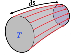
Figure 1: Magnetic Flux Tube. Magnetic flux tube transversal to an open surface $T.$ The magnetic field lines are plotted in red. Arclength element $ds$ along the field-lines is indicated.

surface $T$ of plasma fluid elements. This slip-velocity within the flux tube does, of course, depend upon the particular cross-sectional surface $T$ that is chosen. The properties of $T$ required for this definition of flux-tube velocities will be generally preserved by turbulent flow only for a short time. That is, the surface $T_{t^{\prime}}=\hbox{\boldmath${\mathit{\xi}}$}(t^{\prime};T,t)$ advected by the fluid flow to time $t^{\prime}>t$ will rapidly become wrinkled and folded by turbulent advection. Since the “frozen-in” property does not hold in the turbulent flow, the magnetic field-lines at the later time $t^{\prime}$ may intersect the warped surface $T_{t^{\prime}}$ at multiple points or tangentially. In that case, the slip-velocity of lines anchored to $T_{t^{\prime}}$ is no longer well-defined throughout the tube (although slip-velocities can still be defined for field-lines anchored to individual plasma fluid elements of $T_{t^{\prime}}$, as in the previous section). Only for very narrow flux-tubes, with dimensions of the initial surface $T$ very small (diameters well below the “inner” length $\ell_{d}$), can the flux-tube velocity be defined over extended periods of time.

Under the above restrictive assumptions and with a very special choice of $T,$ it is possible to integrate exactly our equation (3.8) for slip-velocities within the flux-tube, in terms of the so-called “quasi-potential” of General Magnetic Reconnection theory (Schindler et al., 1988; Hesse & Schindler, 1988; Priest et al., 2003). This quantity $V$ is defined for points ${\textit{{x}}}^{\prime}$ within the flux-tube by integrating the parallel electric field $E_{\|}=R_{\|}$ a distance $s$ along the line starting at the unique point x where field-line $L$ through ${\textit{{x}}}^{\prime}$ intersects $T$:

$$V({\textit{{x}}}^{\prime}) = \int_{0}^{s}E_{\|}(\hbox{\boldmath${\mathit{\xi}}$}(s^{\prime};{\textit{{x}}},t),t)ds^{\prime}$$ (3.34)

$$= \int_{L:{\textit{{x}}}\rightarrow{\textit{{x}}}^{\prime}}{\textit{{E}}}(\hbox{\boldmath${\mathit{\xi}}$},t)\hbox{\boldmath$\cdot$}d\hbox{\boldmath${\mathit{\xi}}$}.$$ (3.35)

We prefer to use the more descriptive term “line-voltage” for this quantity. Notice in this setting that the line-voltage $V$ depends upon the distance $s$ along the field-line from $T.$ Now, under the stated assumptions, it is not hard to show (see section 3.2.2 immediately below) that

$$\Delta{\textit{{w}}}_{\perp}=\frac{\hat{{\textit{{B}}}}\hbox{\boldmath$\times$}(\hbox{\boldmath${\mathit{\nabla}}$}V-{\textit{{R}}})}{|{\textit{{B}}}|}.$$ (3.36)

gives an exact solution inside the flux tube to the basic equation (3.8). The solution depends upon the particular cross-section $T$ of the flux tube which is adopted. The natural choice for $T$ is a normal surface to the vector field R, which is transversal to the magnetic field if $R_{\|}\neq 0$ everywhere on the surface. If $T$ is chosen to be such a normal surface of R then it can be seen from (3.36) that $\Delta{\textit{{w}}}_{\perp}=\hbox{\boldmath$0$}$ on $T,$ and hence (3.36) inside the tube indeed gives the slip velocity for field-lines anchored in $T.$ Of course, such a choice of $T$ can only be made instantaneously, since the advected surface $T_{t^{\prime}}$ for $t^{\prime}>t$ will not usually be a normal surface for ${\textit{{R}}}({\textit{{x}}},t^{\prime}).$ The condition of normality becomes vacuous, on the other hand, in a space region where ${\textit{{R}}}\equiv\hbox{\boldmath$0$}$ identically and then any transversal surface $T$ may be selected. We thus recover the results of Priest et al. (2003) for the “standard” situation where the flux tube begins and ends in regions with ${\textit{{R}}}\equiv\hbox{\boldmath$0$}.$

3.2.2 Derivations and Proofs

Here we derive the exact formula (3.36) for the slip-velocity in terms of the line-voltage $V$ within a flux-tube and prove the various statements of the preceding paragraph. The essential observation is that

$$\hat{{\textit{{B}}}},\,\,\,\,{\textit{{z}}}_{\perp}\equiv\hbox{\boldmath${\mathit{\nabla}}$}V-{\textit{{R}}},\,\,\,\,\Delta{\textit{{w}}}_{\perp}\equiv\frac{\hat{{\textit{{B}}}}\hbox{\boldmath$\times$}{\textit{{z}}}_{\perp}}{|{\textit{{B}}}|}$$ (3.37)

form a right-handed orthogonal (but not orthonormal) coordinate system. In particular note

$$\hat{{\textit{{B}}}}\hbox{\boldmath$\cdot$}{\textit{{z}}}_{\perp}=\frac{dV}{ds}-R_{\|}=0.$$ (3.38)

Our strategy shall be to show that $\Delta{\textit{{w}}}_{\perp}$ defined as above satisfies the basic equation (3.8), by verifying the projection of that equation onto each of the above coordinate directions.

For example, differentiating $\hat{{\textit{{B}}}}\hbox{\boldmath$\cdot$}\Delta{\textit{{w}}}_{\perp}=0$ gives

$$\hat{{\textit{{B}}}}\hbox{\boldmath$\cdot$}\frac{d}{ds}(\Delta{\textit{{w}}}_{\perp})=-\Delta{\textit{{w}}}_{\perp}\hbox{\boldmath$\cdot$}\frac{d}{ds}\hat{{\textit{{B}}}}=-\Delta{\textit{{w}}}_{\perp}\hbox{\boldmath$\cdot$}(\hat{{\textit{{B}}}}\hbox{\boldmath$\cdot$}\hbox{\boldmath${\mathit{\nabla}}$})\hat{{\textit{{B}}}},$$ (3.39)

which agrees with the $\hat{{\textit{{B}}}}$-projection of (3.8). This result shows that the term in (3.8) proportional to $(\hat{{\textit{{B}}}}\hat{{\textit{{B}}}})(\hbox{\boldmath${\mathit{\nabla}}$}{\textit{{B}}})$ has a purely geometric origin and is required for that equation to preserve orthogonality with $\hat{{\textit{{B}}}}$ as $\Delta{\textit{{w}}}_{\perp}$ is evolved along the $s$-direction.

Similarly, differentiating ${\textit{{z}}}_{\perp}\hbox{\boldmath$\cdot$}\Delta{\textit{{w}}}_{\perp}=0$ gives

$${\textit{{z}}}_{\perp}\hbox{\boldmath$\cdot$}\frac{d}{ds}(\Delta{\textit{{w}}}_{\perp})=-\Delta{\textit{{w}}}_{\perp}\hbox{\boldmath$\cdot$}\frac{d}{ds}{\textit{{z}}}_{\perp}.$$ (3.40)

To calculate $d{\textit{{z}}}_{\perp}/ds$ we note that

$$\frac{d}{ds}{\textit{{R}}}=(\hat{{\textit{{B}}}}\hbox{\boldmath$\cdot$}\hbox{\boldmath${\mathit{\nabla}}$}){\textit{{R}}}=\partial_{\|}{\textit{{R}}},$$ (3.41)

and the relation $\frac{d}{ds}V=(\hat{{\textit{{B}}}}\hbox{\boldmath$\cdot$}\hbox{\boldmath${\mathit{\nabla}}$})V=R_{\|}$ upon taking the space-gradient yields

$$\frac{d}{ds}\hbox{\boldmath${\mathit{\nabla}}$}V=-(\hbox{\boldmath${\mathit{\nabla}}$}\hat{{\textit{{B}}}})\hbox{\boldmath$\cdot$}\hbox{\boldmath${\mathit{\nabla}}$}V+\hbox{\boldmath${\mathit{\nabla}}$}R_{\|}.$$ (3.42)

Hence, taking the difference of these last two equations,

$$\frac{d}{ds}{\textit{{z}}}_{\perp}=-\hbox{\boldmath${\mathit{\nabla}}$}\hat{{\textit{{B}}}}\hbox{\boldmath$\cdot$}{\textit{{z}}}_{\perp}+(\hbox{\boldmath${\mathit{\nabla}}$}R_{\|}-\partial_{\|}{\textit{{R}}}-\hbox{\boldmath${\mathit{\nabla}}$}\hat{{\textit{{B}}}}\hbox{\boldmath$\cdot$}{\textit{{R}}}).$$ (3.43)

On the other hand, the gradient of the definition $R_{\|}=\hat{{\textit{{B}}}}\hbox{\boldmath$\cdot$}{\textit{{R}}}$ gives

$$\hbox{\boldmath${\mathit{\nabla}}$}R_{\|}=\hbox{\boldmath${\mathit{\nabla}}$}\hat{{\textit{{B}}}}\hbox{\boldmath$\cdot$}{\textit{{R}}}+\hbox{\boldmath${\mathit{\nabla}}$}{\textit{{R}}}\hbox{\boldmath$\cdot$}\hat{{\textit{{B}}}},$$ (3.44)

so that

$$\hbox{\boldmath${\mathit{\nabla}}$}R_{\|}-\partial_{\|}{\textit{{R}}}-\hbox{\boldmath${\mathit{\nabla}}$}\hat{{\textit{{B}}}}\hbox{\boldmath$\cdot$}{\textit{{R}}} = \hbox{\boldmath${\mathit{\nabla}}$}{\textit{{R}}}\hbox{\boldmath$\cdot$}\hat{{\textit{{B}}}}-\partial_{\|}{\textit{{R}}}$$

$$= \left[\hbox{\boldmath${\mathit{\nabla}}$}{\textit{{R}}}-(\hbox{\boldmath${\mathit{\nabla}}$}{\textit{{R}}})^{\top}\right]\cdot\hat{{\textit{{B}}}}$$

$$= \hat{{\textit{{B}}}}\hbox{\boldmath$\times$}(\hbox{\boldmath${\mathit{\nabla}}$}\hbox{\boldmath$\times$}{\textit{{R}}}).$$

It follows that

$$\frac{d}{ds}{\textit{{z}}}_{\perp}=-\hbox{\boldmath${\mathit{\nabla}}$}\hat{{\textit{{B}}}}\hbox{\boldmath$\cdot$}{\textit{{z}}}_{\perp}+\hat{{\textit{{B}}}}\hbox{\boldmath$\times$}(\hbox{\boldmath${\mathit{\nabla}}$}\hbox{\boldmath$\times$}{\textit{{R}}}).$$ (3.45)

Substituting this into (3.40) and using the definition of $\Delta{\textit{{w}}}_{\perp}$ we conclude that

$${\textit{{z}}}_{\perp}\hbox{\boldmath$\cdot$}\frac{d}{ds}(\Delta{\textit{{w}}}_{\perp})={\textit{{z}}}_{\perp}\hbox{\boldmath$\cdot$}\left[(\Delta{\textit{{w}}}_{\perp}\hbox{\boldmath$\cdot$}\hbox{\boldmath${\mathit{\nabla}}$})\hat{{\textit{{B}}}}-\frac{(\hbox{\boldmath${\mathit{\nabla}}$}\hbox{\boldmath$\times$}{\textit{{R}}})_{\perp}}{|{\textit{{B}}}|}\right].$$ (3.46)

This is the ${\textit{{z}}}_{\perp}$-projection of equation (3.8).

Finally, differentiation of $|\Delta{\textit{{w}}}_{\perp}|^{2}=|{\textit{{z}}}_{\perp}|^{2}/|{\textit{{B}}}|^{2}$ gives

$$(\Delta{\textit{{w}}}_{\perp})\hbox{\boldmath$\cdot$}\frac{d}{ds}(\Delta{\textit{{w}}}_{\perp})=\frac{1}{|{\textit{{B}}}|^{2}}{\textit{{z}}}_{\perp}\hbox{\boldmath$\cdot$}\frac{d{\textit{{z}}}_{\perp}}{ds}-\frac{|{\textit{{z}}}_{\perp}|^{2}}{|{\textit{{B}}}|^{2}}\frac{d}{ds}\ln|{\textit{{B}}}|.$$ (3.47)

Using (3.45) for $d{\textit{{z}}}_{\perp}/ds$ gives

$$(\Delta{\textit{{w}}}_{\perp})\hbox{\boldmath$\cdot$}\frac{d}{ds}(\Delta{\textit{{w}}}_{\perp})=-\frac{1}{|{\textit{{B}}}|^{2}}{\textit{{z}}}_{\perp}\hbox{\boldmath$\cdot$}(\hbox{\boldmath${\mathit{\nabla}}$}\hat{{\textit{{B}}}})\hbox{\boldmath$\cdot$}{\textit{{z}}}_{\perp}$$ (3.48)

$$\,\,\,\,\,\,\,\,\,\,\,\,\,\,\,\,\,\,\,\,\,\,\,\,-|\Delta{\textit{{w}}}_{\perp}|^{2}\frac{d}{ds}\ln|{\textit{{B}}}|$$ (3.49)

$$\,\,\,\,\,\,\,\,\,\,\,\,\,\,\,\,\,\,\,\,\,\,\,\,+\frac{1}{|{\textit{{B}}}|^{2}}{\textit{{z}}}_{\perp}\hbox{\boldmath$\cdot$}\hat{{\textit{{B}}}}\hbox{\boldmath$\times$}(\hbox{\boldmath${\mathit{\nabla}}$}\hbox{\boldmath$\times$}{\textit{{R}}}).$$ (3.50)

We next note that a relation on the trace of $\hbox{\boldmath${\mathit{\nabla}}$}\hat{{\textit{{B}}}}$ follows from the solenoidal condition ${\rm Tr}(\hbox{\boldmath${\mathit{\nabla}}$}{\textit{{B}}})=\hbox{\boldmath${\mathit{\nabla}}$}\hbox{\boldmath$\cdot$}{\textit{{B}}}=0,$ by substituting ${\textit{{B}}}=|{\textit{{B}}}|\hat{{\textit{{B}}}}$ to obtain

$${\rm Tr}(\hbox{\boldmath${\mathit{\nabla}}$}\hat{{\textit{{B}}}})=-\frac{d}{ds}\ln|{\textit{{B}}}|.$$ (3.51)

Expressed in terms of the orthogonal coordinate system (3.37), this condition on the trace becomes

$$\frac{1}{|{\textit{{B}}}|^{2}}{\textit{{z}}}_{\perp}\hbox{\boldmath$\cdot$}(\hbox{\boldmath${\mathit{\nabla}}$}\hat{{\textit{{B}}}})\hbox{\boldmath$\cdot$}{\textit{{z}}}_{\perp}+(\Delta{\textit{{w}}}_{\perp})\hbox{\boldmath$\cdot$}(\hbox{\boldmath${\mathit{\nabla}}$}\hat{{\textit{{B}}}})\hbox{\boldmath$\cdot$}(\Delta{\textit{{w}}}_{\perp})$$ (3.52)

$$\,\,\,\,\,\,\,\,\,\,\,\,\,\,\,\,\,\,\,\,\,\,\,\,=-|\Delta{\textit{{w}}}_{\perp}|^{2}\frac{d}{ds}\ln|{\textit{{B}}}|,$$ (3.53)

noting that $(\hbox{\boldmath${\mathit{\nabla}}$}\hat{{\textit{{B}}}})\hbox{\boldmath$\cdot$}\hat{{\textit{{B}}}}=0.$ Using the above trace condition and the definition of $\Delta{\textit{{w}}}_{\perp},$ the equation (3.50) becomes

$$(\Delta{\textit{{w}}}_{\perp})\hbox{\boldmath$\cdot$}\frac{d}{ds}(\Delta{\textit{{w}}}_{\perp})=\,\,\,\,\,\,\,\,\,\,\,\,\,\,\,\,\,\,\,\,\,\,\,\,\,\,\,\,\,\,\,\,\,\,\,\,$$ (3.54)

$$\Delta{\textit{{w}}}_{\perp}\hbox{\boldmath$\cdot$}\left[(\Delta{\textit{{w}}}_{\perp}\hbox{\boldmath$\cdot$}\hbox{\boldmath${\mathit{\nabla}}$})\hat{{\textit{{B}}}}-\frac{(\hbox{\boldmath${\mathit{\nabla}}$}\hbox{\boldmath$\times$}{\textit{{R}}})_{\perp}}{|{\textit{{B}}}|}\right].\,\,\,\,\,\,\,\,\,\,\,\,\,\,\,\,\,\,\,$$ (3.55)

This is the $\Delta{\textit{{w}}}_{\perp}$-projection of equation (3.8).

The formula (3.36) thus solves the equation (3.8) for the line-voltage $V$ developed from any transversal surface $T$ of the flux tube. In order to represent the actual slip velocity $\Delta{\textit{{w}}}_{\perp}$ for field-lines anchored to $T,$ the condition $\Delta{\textit{{w}}}_{\perp}=\hbox{\boldmath$0$}$ must hold on the surface $T.$ This condition is equivalent to $\hbox{\boldmath${\mathit{\nabla}}$}V={\textit{{R}}}$ on $T$. Since $T$ is a zero level-surface of $V,$ by the very definition of $V$, $\hbox{\boldmath${\mathit{\nabla}}$}V$ on $T$ is normal to the surface. Hence, the condition $\hbox{\boldmath${\mathit{\nabla}}$}V={\textit{{R}}}$ can hold on $T$ only if that surface $T$ is chosen to be everywhere normal to ${\textit{{R}}}.$ As a matter of fact, this normality condition is not only necessary but also sufficient to guarantee that $\hbox{\boldmath${\mathit{\nabla}}$}V={\textit{{R}}}$ on $T.$ If the flux tube starts in a region where ${\textit{{R}}}\equiv\hbox{\boldmath$0$},$ then $\hbox{\boldmath${\mathit{\nabla}}$}V={\textit{{R}}}$ trivially. Thus, assume instead that the tube starts in a neighborhood where R is everywhere nonzero, so that the unit vector $\hat{{\textit{{R}}}}$ and its normal surface $T$ are well-defined. In that case, the line-voltage $V$ defined for such a choice of $T$ satisfies

$$\hbox{\boldmath${\mathit{\nabla}}$}V=|\hbox{\boldmath${\mathit{\nabla}}$}V|\hat{{\textit{{R}}}}\,\,\,\,\,\,\,\,{\rm on}\,\,\,\,T.$$ (3.56)

Dotting this equation with $\hat{{\textit{{B}}}}$ and using $dV/ds=R_{\|}$ gives

$$R_{\|}=\hat{{\textit{{B}}}}\hbox{\boldmath$\cdot$}\hbox{\boldmath${\mathit{\nabla}}$}V=|\hbox{\boldmath${\mathit{\nabla}}$}V|(\hat{{\textit{{R}}}})_{\|}=|\hbox{\boldmath${\mathit{\nabla}}$}V|\frac{R_{\|}}{|{\textit{{R}}}|},$$ (3.57)

which implies $|\hbox{\boldmath${\mathit{\nabla}}$}V|=|{\textit{{R}}}|$ on $T$. It follows that

$$\hbox{\boldmath${\mathit{\nabla}}$}V={\textit{{R}}}\,\,\,\,\,\,\,\,{\rm on}\,\,\,\,T$$ (3.58)

and thus $\Delta{\textit{{w}}}_{\perp}=\hbox{\boldmath$0$}$ on $T,$ as claimed.

3.2.3 Discussion of the Results

It is sometimes stated, loosely, that “reconnection occurs when there is a breakdown of ideal MHD and therefore an electric field component ($E_{\|}$) along the magnetic field…” (Priest & Démoulin, 1995). This is an incorrect statement for turbulent reconnection. All current evidence supports the idea that Ohmic electric fields vanish (distributionally) for MHD turbulence in the infinite-conductivity limit, that ideal MHD holds (in the coarse-grained or “weak” sense) and yet reconnection occurs unabated. A more precise statement is that a non-vanishing gradient $\hbox{\boldmath${\mathit{\nabla}}$}V$ is required for reconnection (Schindler et al., 1988; Hesse & Schindler, 1988). It is quite possible that ${\textit{{R}}}\rightarrow\hbox{\boldmath$0$}$ pointwise everywhere, that $V$ vanishes along every field-line segment of finite length, and yet $\hbox{\boldmath${\mathit{\nabla}}$}V$ remains finite or diverges to infinity.

The line-voltage $V$ is sometimes interpreted as a “reconnection rate” or rate of change of magnetic flux due to reconnection. The rationale for this is roughly as follows. Consider points ${\textit{{x}}}^{\prime}$ and ${\textit{{y}}}^{\prime}$ inside the flux tube which are connected by a curve $C^{\prime}$ everywhere orthogonal to B and which have base-points x and y in $T.$ Then the quantity defined by

$$\dot{\Phi}_{{\rm slip}}\equiv\int_{C^{\prime}:{\textit{{x}}}^{\prime}\rightarrow{\textit{{y}}}^{\prime}}{\textit{{B}}}\hbox{\boldmath$\cdot$}(\Delta{\textit{{w}}}_{\perp}\hbox{\boldmath$\times$}d{\textit{{r}}})$$ (3.59)

is naturally interpreted as the rate of transfer across $C^{\prime}$ of the magnetic flux in the tube, due to slippage motion of field-lines. Using (3.36) it is easy to see that

$$\dot{\Phi}_{{\rm slip}}=V({\textit{{x}}}^{\prime})-V({\textit{{y}}}^{\prime})+\int_{C^{\prime}:{\textit{{x}}}^{\prime}\rightarrow{\textit{{y}}}^{\prime}}{\textit{{R}}}\hbox{\boldmath$\cdot$}d{\textit{{r}}}.$$ (3.60)

In the “standard situation” where $C^{\prime}$ is outside an assumed well-localized “diffusion region”, so that ${\textit{{R}}}=\hbox{\boldmath$0$}$ on $C^{\prime},$ the rate of transfer of flux by slippage is simply the difference of the line-voltages, $V({\textit{{x}}}^{\prime})-V({\textit{{y}}}^{\prime}),$ and $V({\textit{{x}}}^{\prime}),V({\textit{{y}}}^{\prime})$ become independent of distance $s$ along the field line. If furthermore ${\textit{{y}}}^{\prime}$ is on a line that lies entirely outside the “diffusion region”, then $V({\textit{{y}}}^{\prime})=0$. In that case, $\dot{\Phi}_{{\rm slip}}=V({\textit{{x}}}^{\prime}),$ so that the rate of change of flux may be identified with $V({\textit{{x}}}^{\prime}).$

None of these statements hold obviously in a turbulent regime with ${\textit{{R}}}\rightarrow\hbox{\boldmath$0$}$. Both $V$ and the line-integral of R along $C^{\prime}$ may vanish. This is not required, of course. Even if ${\textit{{R}}}\rightarrow\hbox{\boldmath$0$}$ almost everywhere in space (with respect to Lebesgue measure) as conductivity goes to infinity, there may be uncountably many field-lines, densely distributed in space, where the line-voltages do not vanish, due to spatial intermittency effects. But in that case, there is no reason that the line-integral of R along $C^{\prime}$ necessarily vanishes either! It is not clear whether $V$ may remain non-zero in high-conductivity MHD turbulence for some subset of lines and, if so, whether these values represent “reconnection rates” along the corresponding segment of these lines. It is one of the open issues in turbulent reconnection whether line-voltages may remain non-vanishing at infinite conductivity for certain lines due to spatial intermittency effects.

It is quite possible, however, that $V\rightarrow 0$ for all field-lines and yet flux-conservation is violated throughout the turbulent flow. Notice that the transfer of magnetic flux within the tube by slippage can be rewritten as

$$\dot{\Phi}_{{\rm slip}}=\oint_{\Gamma}{\textit{{R}}}\hbox{\boldmath$\cdot$}d{\textit{{r}}},$$ (3.61)

where $\Gamma:{\textit{{x}}}\stackrel{{\scriptstyle L_{x}}}{{\rightarrow}}{\textit{{x}}}^{\prime}\stackrel{{\scriptstyle C^{\prime}}}{{\rightarrow}}{\textit{{y}}}^{\prime}\stackrel{{\scriptstyle-L_{y}}}{{\rightarrow}}{\textit{{y}}}\stackrel{{\scriptstyle-C}}{{\rightarrow}}{\textit{{x}}}$ is the closed loop obtained by following up along field-line $L_{x}$ from ${\textit{{x}}}\rightarrow{\textit{{x}}}^{\prime},$ across along $C^{\prime}$ from ${\textit{{x}}}^{\prime}\rightarrow{\textit{{y}}}^{\prime},$ down along line $L_{y}$ from ${\textit{{y}}}^{\prime}\rightarrow{\textit{{y}}},$ and back along $C$ from ${\textit{{y}}}\rightarrow{\textit{{x}}}$ inside $T.$ Here $\int_{C}{\textit{{R}}}\hbox{\boldmath$\cdot$}d{\textit{{r}}}=0$ because $T$ is normal to ${\textit{{R}}}.$ Thus, $\dot{\Phi}_{{\rm slip}}=\left.\frac{d}{dt}\Phi(\Gamma,t)\right|_{t=0}$ represents instantaneous non-conservation of flux through the loop $\Gamma$ due to the non-ideality. However, flux-conservation is a Lagrangian statement and requires that $\frac{d}{dt}\Phi(\Gamma,t)=\oint_{\Gamma(t)}{\textit{{R}}}({\textit{{r}}},t)\hbox{\boldmath$\cdot$}d{\textit{{r}}}$ vanish for the advected loop $\Gamma(t)$ moving with the plasma fluid, at all times $t$. As discussed in Eyink & Aluie (2006), the loop $\Gamma(t)$ for any $t>0$ is expected to approach a non-rectifiable (fractal) curve in the limit of very long inertial ranges. Thus, it is possible that $V\rightarrow 0$ and $\dot{\Phi}_{{\rm slip}}\rightarrow 0$ but that $\frac{d}{dt}\Phi(\Gamma,t)\neq 0$ at positive times $t>0,$ because the vanishing of R is compensated by the unbounded growth of the length of $\Gamma(t)$ as the inertial range increases in extent.

A final remark concerns the behavior of the slip velocity at magnetic nulls. It follows from (3.36) that $\Delta{\textit{{w}}}_{\perp}$ will generally diverge at nulls, unless it happens that the magnitude of $(\hbox{\boldmath${\mathit{\nabla}}$}V-{\textit{{R}}})$ vanishes at an equal or faster rate than $|{\textit{{B}}}|$ as the null is approached. A small flux-tube around a field-line that enters a null along a “spine” will impinge on the “fan” plane and define $V$, at most, in a narrowing layer on that side of the “fan”. $\hbox{\boldmath${\mathit{\nabla}}$}V$ is then defined only in a one-sided sense on the “fan” plane. On the other hand, a small flux-tube around a field-line entering a null inside a “fan” plane will generally lead to a $V$ which is discontinuous at the null and multi-valued on the outgoing “spine”, since each flux-tube line that belongs to the “fan” will usually enter the null with a different voltage.

4 Weak Solutions and Coarse-Grained Generalized Ohm’s Law

We have argued in the previous sections that reconnection is associated fundamentally to the slip-source ${\mathit{\Sigma}}$ and not to the non-ideal electric field ${\textit{{R}}}.$ In particular, the example of resistive MHD turbulence shows that it is possible for R to go to zero (in r.m.s.) and for ${\mathit{\Sigma}}$ to become simultaneously unboundedly large. This fact implies that situations can exist where ideal MHD is valid, but magnetic reconnection will occur freely. This may sound contradictory, but it is only because the sense of validity of ideal MHD for turbulent solutions is in a “weak” or “coarse-grained” sense, which is quite different than the usual notion of validity for smooth, laminar solutions. In this section, we shall explain “weak solutions” in a non-technical manner, relating them to the more physically familiar ideas of spatial coarse-graining and renormalization-group theory.

Furthermore, we shall argue in detail for the validity of ideal Ohm’s law in this “weak” or “coarse-grained” sense, for the modes at length-scales within an MHD-like turbulent inertial-range. We do so by means of an analysis of the Generalized Ohm’s Law for an electron-ion plasma. The plasma (ion) momentum equation could be treated similarly, but, since our primary interest is reconnection, we do not consider it here. The principal example we have in mind is the solar wind, where detailed empirical evidence is available to support our argument.

4.1 Weak Solutions and Spatial Coarse-Graining

The MHD equations and related hydromagnetic equations such as 2-fluid models are conservations laws (for mass, momentum, energy and magnetic field). Thus, they have a standard weak formulation (Evans, 2010). This notion is perhaps most familiar to space scientists and astrophysicists in the context of discontinuous solutions of ideal MHD, such as fast/slow shocks and rotational/tangential discontinuities, and numerical methods to solve for such solutions (LeVeque et al., 1998). It is also understood that turbulence is described by such weak solutions of ideal fluid equations, as suggested originally by Onsager for hydrodynamic turbulence (Onsager, 1949; Eyink & Sreenivasan, 2006; Eyink, 2008; De Lellis & Székelyhidi Jr., 2012) and later by others for MHD turbulence and reconnection (Caflisch et al., 1997; Eyink & Aluie, 2006). Here we give a brief self-contained discussion.

Using as an example the magnetic induction equation

$$\partial_{t}{\textit{{B}}}=-\hbox{\boldmath${\mathit{\nabla}}$}\hbox{\boldmath$\times$}{\textit{{E}}},$$ (4.1)

the weak formulation corresponds to smearing with a smooth test function $\varphi({\textit{{r}}},s)$ and moving all derivatives to the test function:

$$\int d^{3}r\int ds\,\big{[}\partial_{s}\varphi({\textit{{r}}},s){\textit{{B}}}({\textit{{r}}},s)\,\,\,\,\,\,\,\,\,\,\,\,\,\,\,\,\,\,\,\,\,\,\,\,\,\,\,\,\,\,\,\,\,\,\,\,\,\,\,\,\,\,\,\,\,\,\,\,$$ (4.2)

$$\,\,\,\,\,\,\,\,\,\,\,\,\,\,\,\,\,\,\,\,\,\,\,\,\,\,\,\,\,\,\,\,\,\,\,\,+\hbox{\boldmath${\mathit{\nabla}}$}\varphi({\textit{{r}}},s)\hbox{\boldmath$\times$}{\textit{{E}}}({\textit{{r}}},s)\big{]}=0.$$ (4.3)

This notion extends the meaning of “solution” to singular fields ${\textit{{E}}},{\textit{{B}}}$ for which ordinary classical derivatives do not exist. As a matter of fact, it is often sufficient to smear only in the space-variable. Using a sequence of test functions $\phi({\textit{{r}}},s)$ that approximate $\psi({\textit{{r}}})\chi_{[0,t]}(s),$ with $\chi_{[0,t]}(s)$ the characteristic function of the time-interval $[0,t],$ one obtains

$$\int d^{3}r\ \psi({\textit{{r}}}){\textit{{B}}}({\textit{{r}}},t)=\int d^{3}r\,\psi({\textit{{r}}}){\textit{{B}}}_{0}({\textit{{r}}})\,\,\,\,\,\,\,\,\,\,\,\,\,\,\,\,\,\,\,\,\,\,\,\,$$ (4.4)

$$\,\,\,\,\,\,\,\,\,\,\,\,\,\,\,\,\,\,\,\,\,\,\,\,-\int_{0}^{t}ds\int d^{3}r\,\hbox{\boldmath${\mathit{\nabla}}$}\psi({\textit{{r}}})\hbox{\boldmath$\times$}{\textit{{E}}}({\textit{{r}}},s)$$ (4.5)

and for almost every time $t$

$$\frac{d}{dt}\int d^{3}r\,\psi({\textit{{r}}}){\textit{{B}}}({\textit{{r}}},t)=-\int d^{3}r\,\hbox{\boldmath${\mathit{\nabla}}$}\psi({\textit{{r}}})\hbox{\boldmath$\times$}{\textit{{E}}}({\textit{{r}}},t),$$ (4.6)

if the righthand-side in the last equation above is Lebesgue-integrable in time.

The above considerations may seem rather technical, but they can be interpreted in a standard physical picture of spatial coarse-graining, if one takes test functions $\psi({\textit{{r}}})$ of the form

$$\psi_{{\textit{{x}}},\ell}({\textit{{r}}})=\ell^{-3}G(({\textit{{r}}}-{\textit{{x}}})/\ell)\equiv G_{\ell}({\textit{{r}}}-{\textit{{x}}})$$ (4.7)

for some smooth, rapidly decaying, non-negative function $G$ with unit integral and $\ell>0$. In that case, the weak formulation implies the equation

$$\partial_{t}\bar{{\textit{{B}}}}_{\ell}({\textit{{x}}},t)=-\hbox{\boldmath${\mathit{\nabla}}$}\hbox{\boldmath$\times$}\bar{{\textit{{E}}}}_{\ell}({\textit{{x}}},t),$$ (4.8)

for the coarse-grained fields at length-scale $\ell$:

$$\bar{{\textit{{B}}}}_{\ell}({\textit{{x}}},t)=\int d^{3}r\ G_{\ell}({\textit{{r}}}){\textit{{B}}}({\textit{{x}}}+{\textit{{r}}},t),$$ (4.9)

and so forth for $\bar{{\textit{{E}}}}_{\ell},$ etc. As a matter of fact, the above coarse-grained equations for all x and $\ell$ are equivalent to the usual weak formulation. We briefly explain this standard fact without elaborate mathematical detail. Note that for a general smooth test function $\psi$

$$\lim_{\ell\rightarrow 0}\int d^{3}x\,\psi({\textit{{x}}})G_{\ell}({\textit{{r}}}-{\textit{{x}}})=\psi({\textit{{r}}}).$$ (4.10)

On the other hand, one can also approximate the convolution integral by a finite Riemann sum,

$$\int d^{3}x\,\psi({\textit{{x}}})G_{\ell}({\textit{{r}}}-{\textit{{x}}})\simeq\sum_{i=1}^{N}(\Delta V)_{i}\psi({\textit{{x}}}_{i})G_{\ell}({\textit{{r}}}-{\textit{{x}}}_{i})$$ (4.11)

converging as $N\rightarrow\infty.$ Hence, by taking a linear combination of the coarse-grained equations at points ${\textit{{x}}}_{i}$ with coefficients $(\Delta V)_{i}\psi({\textit{{x}}}_{i})$ and taking the limits first $N\rightarrow\infty$ and then $\ell\rightarrow 0,$ one recovers the standard weak formulation with an arbitrary smooth test function $\psi.$

The coarse-graining point of view is the more important one for practical applications, because it gives a physical relevance to weak solutions as valid descriptions over a certain range of length-scales. For example, it is widely believed that the ideal Ohm’s law ${\textit{{E}}}=-{\textit{{u}}}\hbox{\boldmath$\times$}{\textit{{B}}}$ is valid in the solar wind at lengths $\ell$ much greater than the ion gyro-radius $\rho_{i}$ (e.g. see Schekochihin et al. (2009) for a detailed discussion). However, the ideal magnetic induction equation cannot hold in the classical sense of partial-differential equations, since the solar wind is observed to have a Kolmogorov-type turbulent inertial range with magnetic energy spectrum $E_{B}(k,t)\sim k_{\perp}^{-5/3}$ down to ion scales, and kinetic turbulence at smaller scales. Thus, fine-scale magnetic gradients $\hbox{\boldmath${\mathit{\nabla}}$}_{\perp}{\textit{{B}}}$ have a spectrum $k_{\perp}^{2}E_{B}(k,t)\sim k_{\perp}^{1/3}$ with increasing r.m.s. contributions up to wave-numbers of order $1/\rho_{i},$ and continuing to grow up to electron scale wavenumbers Sahraoui et al. (2013). Thus, fine-scale magnetic-field gradients will be dominated by modes at electron scales and there is no sense in which the ideal induction equation can hold for the standard sense of derivatives. What is plausible and consistent with observations is instead that the coarse-grained ideal induction equation

$$\partial_{t}\bar{{\textit{{B}}}}_{\ell}=\hbox{\boldmath${\mathit{\nabla}}$}\hbox{\boldmath$\times$}\overline{({\textit{{u}}}\hbox{\boldmath$\times$}{\textit{{B}}})}_{\ell}$$ (4.12)

is valid to a very good approximation for $\ell\gg\rho_{i}.$ In this precise sense, the ideal induction equation is valid in the “weak sense” for length-scales greater than the ion gyroradius.

This sense of validity has, however, a quite different meaning than the naive validity of the ideal induction equation for the coarse-grained variables $\bar{{\textit{{u}}}}_{\ell},\bar{{\textit{{B}}}}_{\ell}$. In fact, we can rewrite the above equation in terms of the turbulent electric field induced by motions at scales $<\ell$ as

$$\partial_{t}\bar{{\textit{{B}}}}_{\ell}=\hbox{\boldmath${\mathit{\nabla}}$}\hbox{\boldmath$\times$}(\bar{{\textit{{u}}}}_{\ell}\hbox{\boldmath$\times$}\bar{{\textit{{B}}}}_{\ell}+\hbox{\boldmath${\mathit{\varepsilon}}$}_{\ell}),$$ (4.13)

which differs from the naive ideal equation by the apparent “non-ideal” term

$$\hbox{\boldmath${\mathit{\varepsilon}}$}_{\ell}=\overline{({\textit{{u}}}\hbox{\boldmath$\times$}{\textit{{B}}})}_{\ell}-\bar{{\textit{{u}}}}_{\ell}\hbox{\boldmath$\times$}\bar{{\textit{{B}}}}_{\ell}.$$ (4.14)

Yet note that this apparently “non-ideal” electric field is obtained just by coarse-graining the ideal Ohm’s law. The physical meaning is that the turbulent cascade of magnetic energy is governed entirely by ideal MHD-like dynamics. The difference with the naive sense of validity of ideal MHD is, however, the source of many misunderstandings and erroneous conclusions. For example, one often encounters statements like “At $k_{\perp}\rho_{i}\ll 1$, ions … are magnetized and the magnetic field is frozen into the ion flow” (Schekochihin et al., 2009), but they are fundamentally incorrect. Instead, the induced electric field $\hbox{\boldmath${\mathit{\varepsilon}}$}_{\ell}$ in a turbulent environment leads to magnetic reconnection, as was first pointed out, to our knowledge, by Matthaeus & Lamkin (1986).

In the next section below we argue in detail for the validity of (4.12) at length-scales $\ell$ much greater than than the relevant “inner” length-scale $\ell_{d}$ of astrophysical plasma turbulence (the precise length-scale involved depending upon the microscopic plasma properties). Assuming a general, abstract form of Ohm’s law, ${\textit{{E}}}+{\textit{{u}}}\hbox{\boldmath$\times$}{\textit{{B}}}={\textit{{R}}},$ it follows that

$$\partial_{t}\bar{{\textit{{B}}}}_{\ell}=\hbox{\boldmath${\mathit{\nabla}}$}\hbox{\boldmath$\times$}[\overline{({\textit{{u}}}\hbox{\boldmath$\times$}{\textit{{B}}})_{\ell}}+\bar{{\textit{{R}}}}_{\ell}].$$ (4.15)

To obtain (4.12) it is enough for R to vanish in r.m.s magnitude as $\ell_{d}\rightarrow 0.$ To see this, note by an integration by parts that

$$\hbox{\boldmath${\mathit{\nabla}}$}\hbox{\boldmath$\times$}\bar{{\textit{{R}}}}_{\ell}({\textit{{x}}})=\frac{1}{\ell}\int d^{3}r\ (\hbox{\boldmath${\mathit{\nabla}}$}G)_{\ell}({\textit{{r}}})\hbox{\boldmath$\times$}{\textit{{R}}}({\textit{{x}}}+{\textit{{r}}}).$$ (4.16)

Hence, by the Cauchy-Schwartz inequality

$$|\hbox{\boldmath${\mathit{\nabla}}$}\hbox{\boldmath$\times$}\bar{{\textit{{R}}}}_{\ell}({\textit{{x}}})|\leq\frac{1}{\ell}\|(\hbox{\boldmath${\mathit{\nabla}}$}G)_{\ell}\|\cdot\|{\textit{{R}}}\|$$ (4.17)

where $\|{\textit{{R}}}\|=\sqrt{\int d^{3}x\ |{\textit{{R}}}({\textit{{x}}})|^{2}}$ is the space $L^{2}$-norm. This coincides with the r.m.s. magnitude, $R_{rms}=\|{\textit{{R}}}\|$, when the space-average $\int d^{3}x\,{\textit{{R}}}({\textit{{x}}})=\hbox{\boldmath$0$}.$ Hence, if $R_{rms}\rightarrow 0$ as $\ell_{d}\rightarrow 0,$ then $\hbox{\boldmath${\mathit{\nabla}}$}\hbox{\boldmath$\times$}\bar{{\textit{{R}}}}_{\ell}\rightarrow 0$ for every fixed $\ell$ as $\ell_{d}\rightarrow 0.$ Note it is not required here that ${\textit{{R}}}({\textit{{x}}})$ vanish for all ${\textit{{x}}}:$
due to spatial intermittency, there could be non-empty sets of zero volume where ${\textit{{R}}}({\textit{{x}}})\neq\hbox{\boldmath$0$}$ as $\ell_{d}\rightarrow 0.$ The ideal induction equation would still hold in the limit in the “weak” sense. We argued in Section 2 that this situation occurs for resistive MHD with ${\textit{{R}}}=\eta{\textit{{J}}}$, in the limit as $\eta\rightarrow 0.$ Below we argue that the same result holds for more general forms of plasma non-ideality.

4.2 Coarse-Grained Generalized Ohm’s Law

The “weak” validity of the ideal Ohm’s law in an MHD-like inertial range such as the solar wind can be understood starting from the “Generalized Ohm’s Law” of plasma physics, which is, we recall, a rewriting of the electron momentum equation that ignores terms of order $O(m_{e}/m_{i}),$ the electron-ion mass ratio. We have so far in this paper used dimensionless variables with an MHD scaling, but we now write the generalized Ohm’s law in dimensional cgs units, as

$${\textit{{E}}}+\frac{1}{c}{\textit{{u}}}\hbox{\boldmath$\times$}{\textit{{B}}}=\eta{\textit{{J}}}+\frac{1}{nec}{\textit{{J}}}\hbox{\boldmath$\times$}{\textit{{B}}}-\frac{1}{ne}\hbox{\boldmath${\mathit{\nabla}}$}\hbox{\boldmath$\cdot$}{\textbf{P}}_{e}\,\,\,\,\,\,\,\,\,\,\,\,\,\,\,\,\,\,$$ (4.18)

$$+\frac{m_{e}}{ne^{2}}\left[\frac{\partial{\textit{{J}}}}{\partial t}+\hbox{\boldmath${\mathit{\nabla}}$}\hbox{\boldmath$\cdot$}\left({\textit{{J}}}{\textit{{u}}}+{\textit{{u}}}{\textit{{J}}}-\frac{1}{ne}{\textit{{J}}}{\textit{{J}}}\right)\right].$$ (4.19)

This equation has often been used in discussions of magnetic reconnection (Vasyliunas, 1975; Bhattacharjee et al., 1999; Craig & Watson, 2003), where the final term in the square bracket is frequently omitted under the assumption that $J\ll neu.$ On the other hand, a recent paper of Ohia et al. (2012) studies magnetic reconnection using a fluid model that retains only the first and fourth terms in the square bracket and which gives results in good agreement with PIC simulations of kinetic reconnection. We therefore keep all four bracketed terms here. The coarse-grained version of this equation is

$$\bar{{\textit{{E}}}}_{\ell}+\frac{1}{c}\bar{{\textit{{u}}}}_{\ell}\hbox{\boldmath$\times$}\bar{{\textit{{B}}}}_{\ell}=-\hbox{\boldmath${\mathit{\varepsilon}}$}_{\ell}+\eta\bar{{\textit{{J}}}}_{\ell}\,\,\,\,\,\,\,\,\,\,\,\,\,\,\,\,\,\,\,\,\,\,\,\,\,\,\,\,\,\,\,\,\,\,\,\,\,\,\,\,\,\,\,\,\,\,\,\,\,\,\,\,\,\,$$ (4.20)

$$\,\,\,\,\,\,\,\,\,\,\,\,\,\,\,\,\,\,+\frac{1}{nec}\overline{({\textit{{J}}}\hbox{\boldmath$\times$}{\textit{{B}}})_{\ell}}-\frac{1}{ne}\hbox{\boldmath${\mathit{\nabla}}$}\hbox{\boldmath$\cdot$}{\overline{\textbf{P}}}_{e,\ell}\,\,\,\,\,\,\,\,\,\,\,\,\,\,\,\,\,\,$$ (4.21)

$$+\frac{m_{e}}{ne^{2}}\left[\frac{\partial\bar{{\textit{{J}}}}_{\ell}}{\partial t}+\hbox{\boldmath${\mathit{\nabla}}$}\hbox{\boldmath$\cdot$}\overline{\left({\textit{{J}}}{\textit{{u}}}+{\textit{{u}}}{\textit{{J}}}-\frac{1}{ne}{\textit{{J}}}{\textit{{J}}}\right)_{\ell}}\right].$$ (4.22)

Here we assume for simplicity of presentation that the density $n$ is spatially constant, otherwise density-weighted Favre-averging is required (Favre, 1969; Aluie, 2013). For that analysis, see Appendix A. As we shall now show in detail, the dominant term on the righthand side at length-scales $\ell$ in an MHD-like inertial range is the first term $-\hbox{\boldmath${\mathit{\varepsilon}}$}_{\ell}$ from ideal Ohm’s law and all of the other terms are negligible. The reason is that all of the genuinely non-ideal terms involve at least one overall space-gradient. This is obvious for all of the terms except the Hall electric field, where it follows from the non-relativistic Ampere’s law ${\textit{{J}}}=\frac{c}{4\pi}\hbox{\boldmath${\mathit{\nabla}}$}\hbox{\boldmath$\times$}{\textit{{B}}},$ the standard vector calculus identity

$$(\hbox{\boldmath${\mathit{\nabla}}$}\hbox{\boldmath$\times$}{\textit{{B}}})\hbox{\boldmath$\times$}{\textit{{B}}}=({\textit{{B}}}\hbox{\boldmath$\cdot$}\hbox{\boldmath${\mathit{\nabla}}$}){\textit{{B}}}-\frac{1}{2}\hbox{\boldmath${\mathit{\nabla}}$}(|{\textit{{B}}}|^{2}),$$ (4.23)

and the solenoidality condition $\hbox{\boldmath${\mathit{\nabla}}$}\hbox{\boldmath$\cdot$}{\textit{{B}}}=0.$ Each overall space-gradient ${\mathit{\nabla}}$ brings in a factor $\ell^{-1}$ upon coarse-graining at scale $\ell,$ and thus terms with overall gradients give diminishing contributions for increasing $\ell.$ These terms are thus essentially “irrelevant” variables in the renormalization-group sense as the generalized Ohm’s law is coarse-grained to successively larger length-scales. To make more quantitative estimates, one must compare $\ell$ with other relevant length-scales, as we now do term-by-term. Because there is no small parameter on which to base an expansion, our analysis is non-perturbative and exploits an exact cumulant or linked-cluster expansion of coarse-graining averages. See Appendix B for details.

4.2.1 Turbulent subscale electric field

The leading order term in an MHD-like inertial range is the electric field induced by motion of eliminated turbulent eddies at scales $<\ell$, which (see Eyink & Aluie (2006) and Appendix B) can be written in terms of field increments $\delta{\textit{{B}}}({\textit{{r}}};{\textit{{x}}})={\textit{{B}}}({\textit{{x}}}+{\textit{{r}}})-{\textit{{B}}}({\textit{{x}}}),$ etc. as

$$\!\!\!\!\!\!\!\!\!\!\!\!\!\!\!\!\hbox{\boldmath${\mathit{\varepsilon}}$}_{\ell}=\frac{1}{c}\left[\int d^{3}r\,G_{\ell}({\textit{{r}}})\,\delta{\textit{{u}}}({\textit{{r}}})\hbox{\boldmath$\times$}\delta{\textit{{B}}}({\textit{{r}}})\right.\,\,\,\,\,\,\,\,\,\,\,\,\,\,\,\,\,\,\,\,\,\,\,\,\,\,\,\,\,\,\,\,\,\,\,$$ (4.24)

$$\!\!\!\!\!\!\!\!\!\!\!\!\!\!\!\!\!-\left.\int d^{3}r\int d^{3}r^{\prime}\,G_{\ell}({\textit{{r}}})G_{\ell}({\textit{{r}}}^{\prime})\,\delta{\textit{{u}}}({\textit{{r}}})\hbox{\boldmath$\times$}\delta{\textit{{B}}}({\textit{{r}}}^{\prime})\right].$$ (4.25)

In this expression and following ones the x-variable for simplicity is not written explicitly. It is easily seen from this expression for a spherically-symmetric filter kernel $G$ that

$$\hbox{\boldmath${\mathit{\varepsilon}}$}_{\ell}\sim\frac{1}{c}\langle\delta{\textit{{u}}}(\hbox{\boldmath$\ell$})\hbox{\boldmath$\times$}\delta{\textit{{B}}}(\hbox{\boldmath$\ell$})\rangle_{{\rm ang}},$$ (4.26)

where $\langle\cdot\rangle_{{\rm ang}}$ denotes a spherical average over the direction vector $\hat{\hbox{\boldmath$\ell$}}.$ This will be the same order of magnitude as

$$\hbox{\boldmath${\mathit{\varepsilon}}$}_{\ell}\sim\frac{1}{c}\delta u(\ell)\cdot\delta B(\ell),$$ (4.27)

unless the vectors $\delta{\textit{{u}}}(\hbox{\boldmath$\ell$})$, $\delta{\textit{{B}}}(\hbox{\boldmath$\ell$})$ exhibit “dynamic alignment,” which may cause them to be nearly parallel (Boldyrev, 2005, 2006). There is some evidence for this phenomenon in the solar wind (Podesta et al., 2009; Hnat et al., 2011; Wicks et al., 2013b), but dynamic alignment, if it really occurs for $\ell$ much smaller than the turbulent outer scale $L,$ only leads to a reduction by some factor $(\ell/L)^{\beta},$ with $\beta=1/4$ a popular value (Boldyrev, 2006). As we shall see below, this modest reduction does not affect our conclusion that $\hbox{\boldmath${\mathit{\varepsilon}}$}_{\ell}$ is the leading term.

4.2.2 Ohmic electric field

Next consider the Ohmic electric field ${\textit{{E}}}^{{\rm Ohm}}=\eta{\textit{{J}}}$. This contribution is quite tiny in the nearly collisionless solar wind, but it can be the leading non-ideal term in other cases, such as the solar photosphere. The Ohmic field coarse-grained to length $\ell$ can be written in terms of the magnetic increment as

$$\bar{{\textit{{E}}}}_{\ell}^{{\rm Ohm}}=\frac{\lambda}{\ell c}\int d^{3}r(\hbox{\boldmath${\mathit{\nabla}}$}G)_{\ell}({\textit{{r}}})\hbox{\boldmath$\times$}\delta{\textit{{B}}}({\textit{{r}}}),$$ (4.28)

with $\lambda=\eta c^{2}/4\pi$ the magnetic diffusivity. The magnitude of the Ohmic electric field is thus

$$\bar{E}_{\ell}^{{\rm Ohm}}\sim\lambda\frac{\delta B(\ell)}{\ell c}.$$ (4.29)

Taking into account scale-dependent anisotropy as proposed by Goldreich & Sridhar (1995), the $\ell$ in the prefactor of this and other estimates should be interpreted as $\ell_{\perp},$ since the increments that make the largest contributions are those with ${\textit{{r}}}\perp\bar{{\textit{{B}}}}_{\ell}.$ In absence of dynamic alignment, the coarse-grained Ohmic field thus matches the turbulent electric field when $\ell_{\perp}\delta u(\ell)\sim\lambda,$ which is the condition defining the resistive dissipation length $\ell_{\eta}.$ For example, assuming Goldreich-Sridhar scaling $\delta u(\ell)\sim(\varepsilon\ell_{\perp})^{1/3},$ with $\varepsilon$ the energy cascade rate, the resistive dissipation length is $\ell_{\eta,\perp}\sim(\lambda^{3}/\varepsilon)^{1/4}.$ At length-scales $\ell_{\perp}\gg\ell_{\eta,\perp}$ the turbulent electric field is therefore much larger than the Ohmic field. Dynamic alignment changes the velocity scaling to $\delta u(\ell)\sim(\varepsilon\ell_{\perp}^{1-\beta}L^{\beta})^{1/3},$ and thus the resistive dissipation length to $\ell_{\eta,\perp}\sim(\lambda^{3}/\varepsilon L^{\beta})^{1/(4-\beta)}.$ The situation is qualitatively unchanged, with the turbulent field again dominating for $\ell_{\perp}\gg\ell_{\eta,\perp}.$

4.2.3 Hall electric field

The coarse-grained Hall electric field has two contributions, a resolved part

$$\frac{1}{nec}\bar{{\textit{{J}}}}_{\ell}\hbox{\boldmath$\times$}\bar{{\textit{{B}}}}_{\ell}$$ (4.30)

and a Hall contribution to the subscale electric field

$$\hbox{\boldmath${\mathit{\varepsilon}}$}_{\ell}^{{\rm Hall}}=\frac{1}{nec}\left[\overline{({\textit{{J}}}\hbox{\boldmath$\times$}{\textit{{B}}})_{\ell}}-\overline{{\textit{{J}}}}_{\ell}\hbox{\boldmath$\times$}\overline{{\textit{{B}}}}_{\ell}\right].$$ (4.31)

The resolved Hall field can be neglected relative to $\frac{1}{c}\bar{{\textit{{u}}}}_{\ell}\hbox{\boldmath$\times$}\bar{{\textit{{B}}}}_{\ell},$ since $\bar{{\textit{{u}}}}_{\ell}$ is much larger than ${\textit{{u}}}_{\ell}^{{\rm Hall}}\equiv\bar{{\textit{{J}}}}_{\ell}/ne.$ In fact, using the previous estimate that $\delta\bar{J}_{\ell}\sim c\delta B(\ell)/{4\pi\ell_{\perp}},$ one finds that

$$\bar{u}_{\ell}^{{\rm Hall}}/\bar{u}_{\ell}\sim\left(\frac{v_{A}}{\bar{u}_{\ell}}\right)\left(\frac{\delta_{i}}{\ell}\right)\left(\frac{\delta B(\ell)}{B_{0}}\right),$$ (4.32)

where $v_{A}=B_{0}/\sqrt{4\pi m_{i}n}$ is the Alfvén speed based on the mean magnetic field $B_{0}$ and $\delta_{i}=c(m_{i}/4\pi ne^{2})^{1/2}$ is the ion skin depth. In the turbulent inertial range $\delta B(\ell)/B_{0}\ll 1.$ The ratio $v_{A}/\bar{u}_{\ell}$ is a constant factor, which is less than one in super-Alfvénic flow such as the solar wind at 1 AU. Finally, at inertial-range lengths $\ell\gg\delta_{i},$ the other factor is also very small.

The subscale Hall term can be estimated as in Eyink et al. (2011) by using the previously stated vector calculus identity (4.23) to write

$$\hbox{\boldmath${\mathit{\varepsilon}}$}_{\ell}^{{\rm Hall}}=\frac{1}{4\pi ne}\left[\hbox{\boldmath${\mathit{\nabla}}$}\hbox{\boldmath$\cdot$}\hbox{\boldmath$\tau$}^{{\rm Max}}_{\ell}-\frac{1}{2}\hbox{\boldmath${\mathit{\nabla}}$}({\rm tr}\,\hbox{\boldmath$\tau$}^{{\rm Max}}_{\ell})\right]$$ (4.33)

where $\hbox{\boldmath$\tau$}^{{\rm Max}}_{\ell}=\overline{({\textit{{B}}}{\textit{{B}}})_{\ell}}-\overline{{\textit{{B}}}}_{\ell}\overline{{\textit{{B}}}}_{\ell}$ is the turbulent Maxwell stress tensor. Note that $\hbox{\boldmath$\tau$}^{{\rm Max}}_{\ell}$ can be easily written in terms of magnetic field increments as

$$\!\!\!\!\!\!\!\!\!\!\!\!\!\!\!\!\!\!\!\!\!\!\!\!\tau^{{\rm Max}}_{\ell,ij}=\int d^{3}r\,G_{\ell}({\textit{{r}}})\delta B_{i}({\textit{{r}}})\delta B_{j}({\textit{{r}}})$$ (4.34)

$$\!\!\!\!\!\!\!\!\!\!\!\!\!\!\!\!\!\!\!\!\!\!\!\!\!-\int d^{3}r\,G_{\ell}({\textit{{r}}})\delta B_{i}({\textit{{r}}})\cdot\int d^{3}r^{\prime}\,G_{\ell}({\textit{{r}}}^{\prime})\delta B_{j}({\textit{{r}}}^{\prime}),$$ (4.35)

but furthermore so can its space-gradient:

$$\!\!\!\!\!\!\!\!\!\!\!\!\!\!\!\!\partial_{k}\tau^{{\rm Max}}_{\ell,ij}=-\frac{1}{\ell}\left[\int d^{3}r\,(\partial_{k}G)_{\ell}({\textit{{r}}})\delta B_{i}({\textit{{r}}})\delta B_{j}({\textit{{r}}})\right.$$ (4.36)

$$\!\!\!\!\!\!\!\!\!\!\!\!\!\!\!\!-\int d^{3}r\,(\partial_{k}G)_{\ell}({\textit{{r}}})\delta B_{i}({\textit{{r}}})\cdot\int d^{3}r^{\prime}\,G_{\ell}({\textit{{r}}}^{\prime})\delta B_{j}({\textit{{r}}}^{\prime})$$ (4.37)

$$\!\!\!\!\!\!\!\!\!\!\!\!\!\!\!\!\left.-\int d^{3}r\,G_{\ell}({\textit{{r}}})\delta B_{i}({\textit{{r}}})\cdot\int d^{3}r^{\prime}\,(\partial_{k}G)_{\ell}({\textit{{r}}}^{\prime})\delta B_{j}({\textit{{r}}}^{\prime})\right].$$ (4.38)

(4.39)

See Appendix B. This last identity gives the estimate

$$\varepsilon_{\ell}^{{\rm Hall}}\sim\frac{1}{4\pi ne}\frac{(\delta B(\ell))^{2}}{\ell_{\perp}}.$$ (4.40)

If possible dynamic alignment is ignored, then $\varepsilon_{\ell}^{{\rm Hall}}\ll\varepsilon_{\ell}$ when

$$\delta u(\ell)\gg\frac{c}{4\pi ne}\frac{\delta B(\ell)}{\ell_{\perp}}\sim\frac{\delta_{i}}{\ell_{\perp}}\cdot\delta b(\ell),$$ (4.41)

where ${\textit{{b}}}={\textit{{B}}}/\sqrt{4\pi m_{i}n}$ is the magnetic field in Alfvén velocity units. Since weakly compressible MHD-like turbulence in the solar wind consists mainly of shear-Alfvén waves with $\delta u(\ell)\sim\delta b(\ell),$ the above inequality is well satisfied for $L\gg\ell_{\perp}\gg\delta_{i}.$ Dynamic alignment, if it occurs, changes the result only slightly, with $\ell_{\perp}\gg\delta_{i}^{1/(1+\beta)}L^{\beta/(1+\beta)}\equiv\delta_{i}^{*}$ now required. While $\delta_{i}^{*}>\delta_{i},$ nevertheless $\delta_{i}^{*}/L=(\delta_{i}/L)^{1/(1+\beta)}\ll 1,$ if $\beta$ is small as expected. We conclude that the Hall electric field contributions can all be neglected for $\ell_{\perp}$ in the MHD inertial range $\delta_{i}^{*}\ll\ell_{\perp}\ll L.$. This conclusion is in agreement with numerical simulations of Hall MHD turbulence, which find that the Hall term has negligible effects at scales greater than the ion skin depth (Dmitruk & Matthaeus, 2006).

4.2.4 Electron pressure-tensor electric field

It is more straightforward to analyze the electric field arising from the electron pressure tensor because this contribution has an explicit overall gradient. Thus,

$$\frac{1}{ne}\hbox{\boldmath${\mathit{\nabla}}$}\hbox{\boldmath$\cdot$}\bar{{\textbf{P}}}_{e,\ell}({\textit{{x}}})=-\frac{1}{ne\,\ell}\int d^{3}r\,(\hbox{\boldmath${\mathit{\nabla}}$}G)_{\ell}({\textit{{r}}})\hbox{\boldmath$\cdot$}{\textbf{P}}_{e}({\textit{{x}}}+{\textit{{r}}})$$ (4.42)

contains at least one factor $\ell^{-1}.$ Notice that we have not replaced ${\textbf{P}}_{e}({\textit{{x}}}+{\textit{{r}}})$ with the increment ${\textbf{P}}_{e}({\textit{{x}}}+{\textit{{r}}})-{\textbf{P}}_{e}({\textit{{x}}}),$ because the electron pressure is a sub-inertial-range quantity with possible rapid variations on electron scales. Thus, ${\textbf{P}}_{e}({\textit{{x}}}+{\textit{{r}}})-{\textbf{P}}_{e}({\textit{{x}}})$ need not be any smaller than ${\textbf{P}}_{e}({\textit{{x}}}+{\textit{{r}}})$. The size of the latter term is often estimated in reconnection discussions (Vasyliunas, 1975; Bhattacharjee et al., 1999; Craig & Watson, 2003) from the assumption that

$$P_{e}\sim P_{i}\sim nm_{i}u_{th}^{2}\sim\frac{ne}{c}\delta_{i}u_{th}B_{th}$$ (4.43)

with $B_{th}=(4\pi m_{i}n)^{1/2}u_{th}$, which implies that

$$\frac{1}{ne}\hbox{\boldmath${\mathit{\nabla}}$}\bar{P}_{e,\ell}({\textit{{x}}})\sim\frac{P_{e}}{ne\,\ell}\sim\left(\frac{\delta_{i}}{\ell}\right)\frac{u_{th}B_{th}}{c}.$$ (4.44)

The electric field from electron pressure gradient is thus suppressed by one factor of $\delta_{i}/\ell$ in an MHD-like inertial-range where $\ell\gg\delta_{i},$ and can be neglected relative to $\hbox{\boldmath${\mathit{\varepsilon}}$}_{\ell}\sim\delta{\textit{{u}}}(\hbox{\boldmath$\ell$})\hbox{\boldmath$\times$}\delta{\textit{{B}}}(\hbox{\boldmath$\ell$})/c.$ Note that the electron pressure tensor need not be isotropic and the above estimate then applies to each individual component of the tensor.

The above estimate may however be improved by more refined evaluation of the electron pressure, using the assumption of a strong ambient magnetic field ${\textit{{B}}}_{0}$. In this limit simple gyrofluid models can be derived, the lowest-order model of which type has often been employed in simulations of magnetic reconnection (Loureiro & Hammett, 2008; Kleva et al., 1995; Grasso et al., 2000). Using this lowest-order gyrofluid model, Bian & Kontar (2010) and Bian et al. (2010) have derived for kinetic Alfvén wave turbulence as in the solar wind that

$$P_{e}=\frac{neB_{0}}{c}\rho_{s}^{2}\omega_{\|}$$ (4.45)

where $\rho_{s}=c_{s}/\Omega_{c,i}$ is the ion gyroradius calculated from the sound speed $c_{s}$ and the ion cyclotron frequency $\Omega_{c,i},$ and $\omega_{\|}$ is the component of the ion fluid vorticity $\hbox{\boldmath${\mathit{\omega}}$}=\hbox{\boldmath${\mathit{\nabla}}$}\hbox{\boldmath$\times$}{\textit{{u}}}$ along the direction of the magnetic field ${\textit{{B}}}_{0}$. In this case, the coarse-grained electric field contribution becomes

$$\!\!\!\!\!\!\!\!\!\!\!\!\frac{1}{ne}\hbox{\boldmath${\mathit{\nabla}}$}\bar{P}_{e,\ell}=-\frac{1}{c}\left(\frac{\rho_{s}}{\ell}\right)^{2}\int d^{3}r\,\delta{\textit{{u}}}({\textit{{r}}})\hbox{\boldmath$\times$}{\textit{{B}}}_{0}\hbox{\boldmath$\cdot$}(\hbox{\boldmath${\mathit{\nabla}}$}\hbox{\boldmath${\mathit{\nabla}}$}G)_{\ell}({\textit{{r}}})$$ (4.46)

$$\,\,\,\,\,\,\,\,\,\,\,\,\,\sim\left(\frac{\rho_{s}}{\ell}\right)^{2}\frac{1}{c}B_{0}\delta u(\ell).$$ (4.47)

Thus, the gyrofluid model predicts that the electron pressure contribution is actually suppressed by the factor $(\rho_{s}/\ell)^{2}$ and is even smaller than implied by the first estimate.

It is worth emphasizing here that, except for the last estimate, all of our coarse-graining analysis is more general than gyrokinetics, because we do not assume a mean magnetic $B_{0}$ stronger than the fluctuations. We have ignored in this section fluctuations in the density (and temperature) for simplicity of presentation, but the analysis of Appendix A includes those effects. The main assumption that we have made which is not required in gyrokinetics is that the electron-ion mass ratio is small, $m_{e}/m_{i}\ll 1,$ but this condition is always satisfied in the solar wind.

4.2.5 First electron inertia contribution

The first contribution to the coarse-grained electric field arising from electron inertia effects can be evaluated using the Maxwell equations to be

$$\frac{m_{e}}{ne^{2}}\frac{\partial\bar{{\textit{{J}}}}_{\ell}}{\partial t} = c\frac{m_{e}}{4\pi ne^{2}}\hbox{\boldmath${\mathit{\nabla}}$}\hbox{\boldmath$\times$}\frac{\partial\bar{{\textit{{B}}}}_{\ell}}{\partial t}$$ (4.51)

$$= -c^{2}\frac{m_{e}}{4\pi ne^{2}}\hbox{\boldmath${\mathit{\nabla}}$}\hbox{\boldmath$\times$}(\hbox{\boldmath${\mathit{\nabla}}$}\hbox{\boldmath$\times$}\bar{{\textit{{E}}}}_{\ell})$$ (4.52)

$$= -\delta_{e}^{2}\hbox{\boldmath${\mathit{\nabla}}$}\hbox{\boldmath$\times$}(\hbox{\boldmath${\mathit{\nabla}}$}\hbox{\boldmath$\times$}\bar{{\textit{{E}}}}_{\ell})$$ (4.53)

with $\delta_{e}$ the electron skin depth. Assuming quasi-neutrality, $\hbox{\boldmath${\mathit{\nabla}}$}\hbox{\boldmath$\cdot$}\bar{{\textit{{E}}}}_{\ell}=0,$ and then one obtains the further simplification that $-\hbox{\boldmath${\mathit{\nabla}}$}\hbox{\boldmath$\times$}(\hbox{\boldmath${\mathit{\nabla}}$}\hbox{\boldmath$\times$}\bar{{\textit{{E}}}}_{\ell})=\triangle\bar{{\textit{{E}}}}_{\ell}.$ In either case, there are now two space-gradients, leading to a suppression by $\ell^{-2}.$ More precisely,

$$\frac{m_{e}}{ne^{2}}\frac{\partial\bar{{\textit{{J}}}}_{\ell}}{\partial t} = \left(\frac{\delta_{e}}{\ell}\right)^{2}\int d^{3}r\,(\triangle G)_{\ell}({\textit{{r}}}){\textit{{E}}}({\textit{{x}}}+{\textit{{r}}})$$ (4.54)

$$\sim \left(\frac{\delta_{e}}{\ell}\right)^{2}\bar{{\textit{{E}}}}_{\ell}$$ (4.55)

and this is much smaller than $\bar{{\textit{{E}}}}_{\ell}$ itself for $\ell\gg\delta_{e}.$

4.2.6 Second electron inertia contribution

The second contribution to the coarse-grained electric field arising from electron inertia effects has two terms, one factorized term and one cumulant term:

$$\frac{m_{e}}{ne^{2}}\hbox{\boldmath${\mathit{\nabla}}$}\hbox{\boldmath$\cdot$}\overline{\left({\textit{{J}}}{\textit{{u}}}+{\textit{{u}}}{\textit{{J}}}\right)_{\ell}}=\frac{m_{e}}{ne^{2}}\hbox{\boldmath${\mathit{\nabla}}$}\hbox{\boldmath$\cdot$}\left(\bar{{\textit{{J}}}}_{\ell}\bar{{\textit{{u}}}}_{\ell}+\bar{{\textit{{u}}}}_{\ell}\bar{{\textit{{J}}}}_{\ell}\right)$$ (4.56)

$$\,\,\,\,\,\,\,\,\,\,\,\,\,\,+\frac{m_{e}}{ne^{2}}\hbox{\boldmath${\mathit{\nabla}}$}\hbox{\boldmath$\cdot$}\left(\tau_{\ell}({\textit{{J}}},{\textit{{u}}})+\tau_{\ell}({\textit{{u}}},{\textit{{J}}})\right)$$ (4.57)

We denote by $\tau_{\ell}(f,g)=\overline{(fg)_{\ell}}-\bar{f}_{\ell}\bar{g}_{\ell}$ the 2nd-order cumulant from coarse-graining.

The factorized term is easily estimated by writing

$$\!\!\!\!\!\!\!\!\!\!\!\!\!\!\hbox{\boldmath${\mathit{\nabla}}$}\hbox{\boldmath$\cdot$}\left(\bar{{\textit{{J}}}}_{\ell}\bar{{\textit{{u}}}}_{\ell}+\bar{{\textit{{u}}}}_{\ell}\bar{{\textit{{J}}}}_{\ell}\right)=(\bar{{\textit{{J}}}}_{\ell}\hbox{\boldmath$\cdot$}\hbox{\boldmath${\mathit{\nabla}}$})\bar{{\textit{{u}}}}_{\ell}$$ (4.58)

$$\,\,\,\,\,\,\,\,\,\,\,\,\,\,+(\hbox{\boldmath${\mathit{\nabla}}$}\hbox{\boldmath$\cdot$}\bar{{\textit{{u}}}}_{\ell})\bar{{\textit{{J}}}}_{\ell}+(\bar{{\textit{{u}}}}_{\ell}\hbox{\boldmath$\cdot$}\hbox{\boldmath${\mathit{\nabla}}$})\bar{{\textit{{J}}}}_{\ell}$$ (4.59)

and by using methods like those previously to show that

$$\hbox{\boldmath${\mathit{\nabla}}$}\bar{{\textit{{u}}}}_{\ell}\sim\frac{\delta u(\hbox{\boldmath$\ell$})}{\ell},\,\,\,\,\hbox{\boldmath${\mathit{\nabla}}$}\bar{{\textit{{J}}}}_{\ell}\sim\frac{c}{4\pi}\frac{\delta B(\hbox{\boldmath$\ell$})}{\ell^{2}}.$$ (4.60)

Hence,

$$\!\!\!\!\!\!\!\!\!\!\!\!\!\!\frac{m_{e}}{ne^{2}}\hbox{\boldmath${\mathit{\nabla}}$}\hbox{\boldmath$\cdot$}\left(\bar{{\textit{{J}}}}_{\ell}\bar{{\textit{{u}}}}_{\ell}+\bar{{\textit{{u}}}}_{\ell}\bar{{\textit{{J}}}}_{\ell}\right)\,\,\,\,\,\,\,\,\,\,\,\,\,\,\,\,\,\,\,\,\,\,\,\,\,\,\,\,$$ (4.61)

$$\!\!\!\!\!\!\!\!\!\!\!\!\!\!\sim\left(\frac{\delta_{e}}{\ell}\right)^{2}\left[\frac{2}{c}\delta u(\ell)\delta B(\ell)+\frac{1}{c}u\,\delta B(\ell)\right]$$ (4.62)

and this electric field is small relative to $\hbox{\boldmath${\mathit{\varepsilon}}$}_{\ell}\sim\delta{\textit{{u}}}(\hbox{\boldmath$\ell$})\hbox{\boldmath$\times$}\delta{\textit{{B}}}(\hbox{\boldmath$\ell$})/c$ for $\ell\gg\delta_{e}.$

The cumulant term is more complex. As shown in Appendix B

$$\!\!\!\!\!\!\!\!\!\!\!\!\!\!\hbox{\boldmath${\mathit{\nabla}}$}\hbox{\boldmath$\cdot$}\tau_{\ell}({\textit{{J}}},{\textit{{u}}})=-\frac{1}{\ell}\left[\int d^{3}r\ (\hbox{\boldmath${\mathit{\nabla}}$}G)_{\ell}({\textit{{r}}})\hbox{\boldmath$\cdot$}\delta{\textit{{J}}}({\textit{{r}}})\delta{\textit{{u}}}({\textit{{r}}})\right.$$ (4.63)

$$\!\!\!\!\!\!\!\!\!\!\!\!\!\!-\int d^{3}r\ (\hbox{\boldmath${\mathit{\nabla}}$}G)_{\ell}({\textit{{r}}})\int d^{3}r^{\prime}\ G_{\ell}({\textit{{r}}}^{\prime})\ \hbox{\boldmath$\cdot$}\delta{\textit{{J}}}({\textit{{r}}})\delta{\textit{{u}}}({\textit{{r}}}^{\prime})$$ (4.64)

$$\!\!\!\!\!\!\!\!\!\!\!\!\!\!\left.-\int d^{3}r\ G_{\ell}({\textit{{r}}})\int d^{3}r^{\prime}\ (\hbox{\boldmath${\mathit{\nabla}}$}G)_{\ell}({\textit{{r}}}^{\prime})\hbox{\boldmath$\cdot$}\delta{\textit{{J}}}({\textit{{r}}})\delta{\textit{{u}}}({\textit{{r}}}^{\prime})\right].$$ (4.65)

However, this yields only one factor $\ell^{-1}.$ Furthermore, J is a very rough field on MHD inertial-range scales and, in collisionless plasmas like the solar wind, even down to electron scales. The lack of any smoothness at inertial-range separations r means that current increments are not small, but instead take on large values $\delta{\textit{{J}}}({\textit{{r}}})\sim{\textit{{J}}}\sim(c/4\pi)\delta B(\delta_{e})/\delta_{e}$ for a collisionless plasma with magnetic fields rough down to the length-scale $\delta_{e}.$ One thus obtains an estimate

$$\frac{m_{e}}{ne^{2}}\hbox{\boldmath${\mathit{\nabla}}$}\hbox{\boldmath$\cdot$}\left(\tau_{\ell}({\textit{{J}}},{\textit{{u}}})+\tau_{\ell}({\textit{{u}}},{\textit{{J}}})\right)\sim\left(\frac{\delta_{e}}{\ell}\right)\cdot\frac{1}{c}\delta u(\ell)\delta B(\delta_{e}).$$ (4.67)

This term is suppressed by only a single factor of $(\delta_{e}/\ell).$ On the other hand, it is also true in the solar wind and other similar cases of collisionless plasma turbulence that $\delta B(\delta_{e})\ll\delta B(\ell)$ for $\ell\gg\delta_{e},$ since $\delta B(\ell)\sim\ell_{\perp}^{h}$ with $h\simeq 1/3$ for $L\gg\ell\gg\delta_{i}$ and $h\simeq 2/3$ for $\delta_{i}\gg\ell\gg\delta_{e}$ (Sahraoui et al., 2013). Thus, there is suppression relative to $\hbox{\boldmath${\mathit{\varepsilon}}$}_{\ell}\sim\delta{\textit{{u}}}(\hbox{\boldmath$\ell$})\hbox{\boldmath$\times$}\delta{\textit{{B}}}(\hbox{\boldmath$\ell$})/c$ by the total factor $\delta_{e}\delta B(\delta_{e})/\ell\delta B(\ell)\ll 1.$

4.2.7 Third electron inertia contribution

The third contribution from electron inertia, $-\frac{1}{n^{2}e^{3}c}\hbox{\boldmath${\mathit{\nabla}}$}\hbox{\boldmath$\cdot$}\overline{\left({\textit{{J}}}{\textit{{J}}}\right)_{\ell}},$ can be understood in a similar fashion to the cumulant term from the second contribution above. Noting that

$$\hbox{\boldmath${\mathit{\nabla}}$}\hbox{\boldmath$\cdot$}\overline{\left({\textit{{J}}}{\textit{{J}}}\right)_{\ell}} = -\frac{1}{\ell}\int d^{3}r\ (\hbox{\boldmath${\mathit{\nabla}}$}G)_{\ell}({\textit{{r}}})\hbox{\boldmath$\cdot$}{\textit{{J}}}({\textit{{x}}}+{\textit{{r}}}){\textit{{J}}}({\textit{{x}}}+{\textit{{r}}})$$ (4.68)

$$\sim \frac{1}{\ell}J^{2}$$ (4.69)

and using the estimate $J\sim(c/4\pi)\delta B(\delta_{e})/\delta_{e},$ one finds that

$$-\frac{1}{n^{2}e^{3}c}\hbox{\boldmath${\mathit{\nabla}}$}\hbox{\boldmath$\cdot$}\overline{\left({\textit{{J}}}{\textit{{J}}}\right)_{\ell}}\sim\left(\frac{\delta_{e}}{\ell}\right)\cdot\frac{1}{c}\frac{(\delta B(\delta_{e}))^{2}}{\sqrt{4\pi m_{i}n}}.$$ (4.70)

If one assumes approximate equipartition of magnetic and velocity fields down to electron scales (Bian & Kontar, 2010), then $\delta u(\delta_{e})\sim\delta b(\delta_{e})=\delta B(\delta_{e})/\sqrt{4\pi m_{i}n}$ and the estimate becomes

$$-\frac{1}{n^{2}e^{3}c}\hbox{\boldmath${\mathit{\nabla}}$}\hbox{\boldmath$\cdot$}\overline{\left({\textit{{J}}}{\textit{{J}}}\right)_{\ell}}\sim\left(\frac{\delta_{e}}{\ell}\right)\cdot\frac{1}{c}\delta u(\delta_{e})\delta B(\delta_{e})$$ (4.71)

and this is smaller than $\hbox{\boldmath${\mathit{\varepsilon}}$}_{\ell}\sim\delta{\textit{{u}}}(\hbox{\boldmath$\ell$})\hbox{\boldmath$\times$}\delta{\textit{{B}}}(\hbox{\boldmath$\ell$})/c$ by the factor $\delta_{e}\delta u(\delta_{e})\delta B(\delta_{e})/\ell\delta u(\ell)\delta B(\ell)\ll 1.$

4.3 The contributions to $\hbox{\boldmath${\mathit{\nabla}}$}\hbox{\boldmath$\times$}\bar{{\textit{{E}}}}_{\ell}$

Having completed our estimate of all the terms in the coarse-grained Generalized Ohm’s Law, we now make a similar estimate of all the terms in the coarse-grained Faraday’s law

$$\partial_{t}\bar{{\textit{{B}}}}_{\ell}=-c\hbox{\boldmath${\mathit{\nabla}}$}\hbox{\boldmath$\times$}\bar{{\textit{{E}}}}_{\ell}.$$ (4.72)

Fortunately, most of the work has already been done in our estimate of the contributions to $\bar{{\textit{{E}}}}_{\ell}.$ As we shall now show, the contributions to $\hbox{\boldmath${\mathit{\nabla}}$}\hbox{\boldmath$\times$}\bar{{\textit{{E}}}}_{\ell}$ differ from the corresponding contributions to $\bar{{\textit{{E}}}}_{\ell}$ only by an additional factor of $\ell^{-1}$

For example, the resolved induction gives

$$\hbox{\boldmath${\mathit{\nabla}}$}\hbox{\boldmath$\times$}(\bar{{\textit{{u}}}}_{\ell}\hbox{\boldmath$\times$}\bar{{\textit{{B}}}}_{\ell})=-(\bar{{\textit{{u}}}}_{\ell}\hbox{\boldmath$\cdot$}\hbox{\boldmath${\mathit{\nabla}}$})\bar{{\textit{{B}}}}_{\ell}+(\bar{{\textit{{B}}}}_{\ell}\hbox{\boldmath$\cdot$}\hbox{\boldmath${\mathit{\nabla}}$})\bar{{\textit{{u}}}}_{\ell}-\bar{{\textit{{B}}}}_{\ell}(\hbox{\boldmath${\mathit{\nabla}}$}\hbox{\boldmath$\cdot$}\bar{{\textit{{u}}}}_{\ell}),$$ (4.73)

which yields the estimate

$$\hbox{\boldmath${\mathit{\nabla}}$}\hbox{\boldmath$\times$}(\bar{{\textit{{u}}}}_{\ell}\hbox{\boldmath$\times$}\bar{{\textit{{B}}}}_{\ell})\sim\frac{1}{\ell}u\delta B(\ell)+\frac{2}{\ell}B\delta u(\ell).$$ (4.74)

The subscale turbulent induction contribution is estimated from the identity

$$\!\!\!\!\!\!\!\!\!\!\!\!c\hbox{\boldmath${\mathit{\nabla}}$}\hbox{\boldmath$\times$}\hbox{\boldmath${\mathit{\varepsilon}}$}_{\ell}=\frac{1}{\ell}\left[\int d^{3}r\ (\hbox{\boldmath${\mathit{\nabla}}$}G)_{\ell}({\textit{{r}}})\hbox{\boldmath$\times$}(\delta{\textit{{u}}}({\textit{{r}}})\hbox{\boldmath$\times$}\delta{\textit{{B}}}({\textit{{r}}}))\right.$$ (4.75)

$$\!\!\!\!\!\!\!\!\!\!\!\!-\int d^{3}r\ (\hbox{\boldmath${\mathit{\nabla}}$}G)_{\ell}({\textit{{r}}})\int d^{3}r^{\prime}\ G_{\ell}({\textit{{r}}}^{\prime})\ \hbox{\boldmath$\times$}(\delta{\textit{{u}}}({\textit{{r}}})\hbox{\boldmath$\times$}\delta{\textit{{B}}}({\textit{{r}}}^{\prime}))$$ (4.76)

$$\!\!\!\!\!\!\!\!\!\!\!\!\left.-\int d^{3}r\ G_{\ell}({\textit{{r}}})\int d^{3}r^{\prime}\ (\hbox{\boldmath${\mathit{\nabla}}$}G)_{\ell}({\textit{{r}}}^{\prime})\ \hbox{\boldmath$\times$}(\delta{\textit{{u}}}({\textit{{r}}})\hbox{\boldmath$\times$}\delta{\textit{{B}}}({\textit{{r}}}^{\prime}))\right].$$ (4.77)

For a spherically symmetric filter kernel, $\hbox{\boldmath${\mathit{\nabla}}$}G(r)=G^{\prime}(r)\hat{{\textit{{r}}}}$ and thus

$$c\hbox{\boldmath${\mathit{\nabla}}$}\hbox{\boldmath$\times$}\hbox{\boldmath${\mathit{\varepsilon}}$}_{\ell}\sim\frac{1}{\ell}\langle\hat{\hbox{\boldmath$\ell$}}\hbox{\boldmath$\times$}(\delta{\textit{{u}}}(\hbox{\boldmath$\ell$})\hbox{\boldmath$\times$}\delta{\textit{{B}}}(\hbox{\boldmath$\ell$}))\rangle_{{\rm ang}}.$$ (4.79)

One can see that these are the dominant contributions to $c\hbox{\boldmath${\mathit{\nabla}}$}\hbox{\boldmath$\times$}\bar{{\textit{{E}}}}_{\ell}.$

Indeed, all of the contributions to $c\hbox{\boldmath${\mathit{\nabla}}$}\hbox{\boldmath$\times$}\bar{{\textit{{E}}}}_{\ell}$ from the non-ideal terms in the Generalized Ohm’s Law can be estimated with the help of the following general identities:

$$\partial_{i_{1}}\cdots\partial_{i_{p}}\bar{f}_{\ell}=\frac{(-1)^{p}}{\ell^{p}}\int d^{3}r\ (\partial_{i_{1}}\cdots\partial_{i_{p}}G)_{\ell}({\textit{{r}}})\,\delta f({\textit{{r}}}),$$ (4.80)

and

$$\!\!\!\!\!\!\!\!\!\!\!\!\partial_{i}\partial_{j}\tau_{\ell}(f,g)=\frac{1}{\ell^{2}}\left[\int d^{3}r\,(\partial_{i}\partial_{j}G)_{\ell}({\textit{{r}}})\delta f({\textit{{r}}})\delta g({\textit{{r}}})\right.$$ (4.81)

$$\!\!\!\!\!\!\!\!\!\!\!\!-\int d^{3}r\int d^{3}r^{\prime}\,(\partial_{i}\partial_{j}G)_{\ell}({\textit{{r}}})G_{\ell}({\textit{{r}}}^{\prime})\,\delta f({\textit{{r}}})\delta g({\textit{{r}}}^{\prime})$$ (4.82)

$$\!\!\!\!\!\!\!\!\!\!\!\!-\int d^{3}r\int d^{3}r^{\prime}\,G_{\ell}({\textit{{r}}})(\partial_{i}\partial_{j}G)_{\ell}({\textit{{r}}}^{\prime})\,\delta f({\textit{{r}}})\delta g({\textit{{r}}}^{\prime})$$ (4.83)

$$\!\!\!\!\!\!\!\!\!\!\!\!-\int d^{3}r\int d^{3}r^{\prime}\,(\partial_{i}G)_{\ell}({\textit{{r}}})(\partial_{j}G)_{\ell}({\textit{{r}}}^{\prime})\,\delta f({\textit{{r}}})\delta g({\textit{{r}}}^{\prime})$$ (4.84)

$$\!\!\!\!\!\!\!\!\!\!\!\!\left.-\int d^{3}r\int d^{3}r^{\prime}\,(\partial_{j}G)_{\ell}({\textit{{r}}})(\partial_{i}\partial_{j}G)_{\ell}({\textit{{r}}}^{\prime})\,\delta f({\textit{{r}}})\delta g({\textit{{r}}}^{\prime})\right].$$ (4.85)

(4.86)

These and other such identities invoked previously can be checked by tedious calculation or derived more conveniently by a cumulant generating function technique (Eyink (2007) and Appendix B). We leave it to the reader to check with these identities that the curl of each of the non-ideal contributions to $\bar{{\textit{{E}}}}_{\ell}$ is modified in magnitude simply by an additional factor of $\ell^{-1}.$ Hence, the relative magnitude of all of the terms is unchanged and the ideal contributions remain the largest to the curl $c\hbox{\boldmath${\mathit{\nabla}}$}\hbox{\boldmath$\times$}\bar{{\textit{{E}}}}_{\ell}.$

From this fact we draw two important conclusions. First, the ideal induction equation is the leading-order dynamical description in the coarse-grained or “weak” sense for length-scales $\ell$ in the turbulent inertial range. This is a very different statement, however, than saying that the coarse-grained variables $\bar{{\textit{{u}}}}_{\ell},\bar{{\textit{{B}}}}_{\ell}$ satisfy the ideal equation in the naive sense. The latter statement overlooks the contribution of the turbulent subscale electric field ${\textit{{R}}}^{T}_{\ell}=-\hbox{\boldmath${\mathit{\varepsilon}}$}_{\ell}$ which appears as an apparent “non-ideal” term in the coarse-grained Ohm’s law but which arises in fact from ideal turbulence dynamics. Second, the leading-order contribution to the slip source $-(\hbox{\boldmath${\mathit{\nabla}}$}\hbox{\boldmath$\times$}\bar{{\textit{{R}}}}_{\ell})_{\perp}/|\bar{{\textit{{B}}}}_{\ell}|$ for lengths in the turbulent inertial range $\ell$, is the ideal MHD term $(\hbox{\boldmath${\mathit{\nabla}}$}\hbox{\boldmath$\times$}\hbox{\boldmath${\mathit{\varepsilon}}$}_{\ell})_{\perp}/|\bar{{\textit{{B}}}}_{\ell}|.$ Despite ideal Ohm’s law holding at those length-scales $\ell$ in the “weak” or coarse-grained sense, field-lines of the coarse-grained magnetic field $\bar{{\textit{{B}}}}_{\ell}$ are not “frozen-in” and the line-slippage at those scales is due to ideal turbulence physics rather than to non-ideal plasma effects.

At length-scale $\ell$ in the inertial range, the slip-velocity acquired along a length $\ell$ of field-line will have magnitude $~{}|\delta{\textit{{u}}}(\hbox{\boldmath$\ell$})\hbox{\boldmath$\times$}\delta{\textit{{B}}}(\hbox{\boldmath$\ell$})|/|\bar{{\textit{{B}}}}_{\ell}|$. Note that this is consistent on order of magnitude with a “turbulent E$\times$B-drift velocity” given by ${\textit{{v}}}_{{\rm slip},\ell}=-c\hbox{\boldmath${\mathit{\varepsilon}}$}_{\ell}\hbox{\boldmath$\times$}\widehat{\bar{{\textit{{B}}}}}_{\ell}/|\bar{{\textit{{B}}}}_{\ell}|$ (Eyink & Aluie, 2006), which will allow lines of the coarse-grained magnetic field $\bar{{\textit{{B}}}}_{\ell}$ to drift relative to the coarse-grained plasma fluid velocity $\bar{{\textit{{u}}}}_{\ell}.$ Here let us just note the exact decomposition of the turbulent emf

$$c\hbox{\boldmath${\mathit{\varepsilon}}$}_{\ell}=\alpha_{\ell}\bar{{\textit{{B}}}}_{\ell}+{\textit{{v}}}_{{\rm slip},\ell}\hbox{\boldmath$\times$}\bar{{\textit{{B}}}}_{\ell},$$ (4.87)

with $\alpha_{\ell}=c\hbox{\boldmath${\mathit{\varepsilon}}$}_{\ell}\hbox{\boldmath$\cdot$}\widehat{\bar{{\textit{{B}}}}}_{\ell}/|\bar{{\textit{{B}}}}_{\ell}|$ a pseudo-scalar field with dimensions of velocity that measures inverse cascade of magnetic helicity/dynamo action. When $\alpha_{\ell}\ll v_{{\rm slip,\ell}},$ one can assign a velocity $\bar{{\textit{{u}}}}_{\ell}+{\textit{{v}}}_{{\rm slip},\ell}$ to magnetic field-lines which is dynamically consistent with the induction equation (Newcomb, 1958). This approach to turbulent-induced slip of field-lines is therefore less general than the slip-velocity source in section 3.1, but it is more practical to apply to the limited (one-dimensional) information available from most single-spacecraft observations of the solar wind, as we see below.

5 Implications for Heliospheric Reconnection

There are important physical implications of the results presented in this paper. We consider here briefly just a few of them.

5.1 Breakdown of the Parker Spiral

We begin with the Parker (1958) spiral model of the interplanetary magnetic field, which is one of the most famous applications in astrophysics and space science of the “frozen-in” principle for magnetic field-lines. The model has been shown to be approximately valid when taking into account solar cycle variations in source magnetic field strength and latitude/time variation in solar wind speeds. Using yearly-averaged magnetic field strengths calculated from observations of Voyager 1 and 2 in the period 1978-2001 at solar distances 1-81 AU and comparing with Parker’s model for estimated magnetic field strength and wind speed on a source surface at 1 AU, Burlaga et al. (2002) found a mean deviation of only -2% between observations and model. On the other hand, typical yearly deviations were around $\pm 20$% and the maximum error (in 1993) was about -40%. These sizable yearly deviations may be partly due to inaccuracies in inputs or errors in observations of the magnetic field, but some part is also clearly due to inaccuracy of the model. For example, there is a clear correlation of the relative error with the solar cycle, with the greatest deviations at years of solar maximum (see Figure 4 of Burlaga et al. (2002)). One should recall that Parker (1958) concluded his paper with a “warning to the reader against taking too literally any of the smooth idealized models which we have constructed in this paper”.

Whereas the study of Burlaga et al. (2002) considered only magnetic field strengths, the earlier work of Burlaga et al. (1982) had studied the magnetic vector geometry and found “notable deviations” from the spiral model. Burlaga et al. (1982) studied daily averages of magnetic field observations of Voyager 1 and 2 in the ecliptic plane at solar distances $R=$1-5 AU during a period of increasing solar activity in the years 1977-1979. In contrast to the Parker predictions for radial magnetic field component radial dependencies $B_{R}\sim R^{-2}$ and azimuthal component $B_{T}\sim R^{-1},$ Burlaga et al. (1982) found $B_{R}\sim R^{-1.56}$ and $B_{T}\sim R^{-1.20}.$ They contrasted their findings with earlier Pioneer 10, 11 investigations between 1 and 8.5 AU during the period 1972-1976 when the sun was less active, which confirmed the spiral model modulo variability on time scales shorter than a solar rotation period. Burlaga et al. (1982) attributed the observed deviations “to temporal variations associated with increasing solar activity, and to the effects of fluctuations of the field in the radial direction.”

These early observations were recently confirmed by Khabarova & Obridko (2012), who presented evidence on the breakdown of the Parker spiral model for time- and space-averaged values of the magnetic field from several spacecraft (Helios 2, Pioneer Venus Orbiter, IMP8, Voyager 1) in the inner heliosphere at solar distances 0.3-5 AU and in the years 1976-1979. This study thus significantly overlapped with that of Burlaga et al. (2002), but used time averages over longer periods (from 76 days to 2 years) coupled with space averages over intervals of width up to 1 AU. For details of the averaging, see Table 1 of Khabarova & Obridko (2012). This more extensive averaging eliminated sizable fluctuations still observed in the daily averages of Burlaga et al. (1982) (see their Figure 1). The study of Khabarova & Obridko (2012) is in essential agreement with Burlaga et al. (1982), finding dependencies $B_{R}\sim R^{-1.66}$ and $B_{T}\sim R^{-1.10},$ just a bit closer to the Parker predictions. Khabarova & Obridko (2012) interpret their observations as due to “a quasi-continuous magnetic reconnection, occurring both at the heliospheric current sheet and at local current sheets inside the IMF sectors”. They present extensive evidence that most nulls of $B_{R}$ and $B_{T},$ where reconnection may occur, are not associated to the heliospheric current sheet. They as well observe a rapid disappearance of the regular sector structure at distances past 1 AU, which they attribute to “turbulent processes in the inner heliosphere.” See also Roberts et al. (2005); Roberts (2010).

This interpretation is consistent with our results, since line-slippage due to pervasive turbulence in the near-ecliptic solar wind will lead to a less tightly wound spiral and a stronger radial field-strength than in the Parker model, as observed by Khabarova & Obridko (2012). This is essentially the same phenomenon as the “reconnection diffusion” proposed by Lazarian (2005) and Santos-Lima et al. (2010), as a mechanism of removal of magnetic fields from collapsing molecular clouds in star formation, and equivalent to the “turbulent E$\times$B-drift” of Eyink & Aluie (2006). The magnitude and direction of the drift velocity at length-scale $\ell$ is given by

$${\textit{{v}}}_{{\rm slip},\ell}=-c\hbox{\boldmath${\mathit{\varepsilon}}$}_{\ell}\hbox{\boldmath$\times$}\widehat{\bar{{\textit{{B}}}}}_{\ell}/|\bar{{\textit{{B}}}}_{\ell}|.$$ (5.1)

As discussed in section 4.2.1, this can be estimated on order of magnitude from the approximate expression

$${\textit{{v}}}_{{\rm slip},\ell} \sim -(\delta{\textit{{u}}}(\hbox{\boldmath$\ell$})\hbox{\boldmath$\times$}\delta{\textit{{B}}}(\hbox{\boldmath$\ell$}))\hbox{\boldmath$\times$}\widehat{\bar{{\textit{{B}}}}}_{\ell}/|\bar{{\textit{{B}}}}_{\ell}|^{2}$$ (5.2)

$$\sim \delta u(\ell)\delta B(\ell)/B_{0}\sim 0.5(\delta B(\ell)/B_{0})^{2}v_{A},$$ (5.3)

with $v_{A}$ the Alfvén speed based on $B_{0}.$ The second line follows by ignoring any suppression due to dynamic alignment effects. It is worth observing that the latter speed $v_{{\rm slip},\ell}$ given by equation (LABEL:vslip-LV99) is numerically identical to the turbulent reconnection speed at perpendicular scale $\ell$ in the theory of Lazarian & Vishniac (1999). Here we have assumed that $\delta u(\ell)/v_{A}\sim 0.5\ \delta B(\ell)/B_{0},$ as is often observed in the inertial range. If $\delta B(\ell)/B_{0}\simeq 1$ for large $\ell$, one can expect $v_{{\rm slip}}\sim v_{A}$.

To give more precise estimates, we appeal to observations. We use two sets of Ulysses data from the “COHOWeb” data sets compiled by J. King at the National Space Science Data Center (NSSDC). One set of data is from polar-latitude fast wind near solar minimum in 1995, on days 100-200 when Ulysses moved between distances 1.36-2.02 AU and heliospheric latitudes $21.3^{\circ}-80.2^{\circ}$. The other set is from near-ecliptic pure slow wind near solar maximum in 1992, on days 151-159 when the spacecraft passed from 5.34 AU to 5.38 AU and from latitude $-10.11^{\circ}$ to $-13.14^{\circ}.$ These two extreme cases should give a good idea of the range of variation of the turbulent drifts. The Ulysses magnetic field data has 1 sec resolution but the plasma data has only 4 min resolution. This is sufficient for our purposes, since we are primarily interested in large lengths $\ell.$ As usual, we can employ Taylor’s hypothesis to interpret time-increments $\tau$ as space-increments $\ell,$ by the formula $\ell=\bar{u}\tau$ where $\bar{u}$ is the mean solar wind speed. This should work well for the very slowly evolving large-scale features that are our principal concern. As a matter of fact, all of our formalism carries over also to time-averaging (Germano, 1992), so that we will present the coarse-grained quantities in terms of time variables. The bulk-averaged properties of the two solar wind cases are presented in Table 1.

Table 1
Parameters for the Two Solar Wind Datasets
Parameter	high-speed	low-speed
velocity magnitude $u$ (km$\,{\rm sec}^{-1}$)	770	430
radial velocity $u_{R}$ (km$\,{\rm sec}^{-1}$)	769	429
tangential velocity $u_{T}$ (km$\,{\rm sec}^{-1}$)	19.4	5.69
normal velocity $u_{N}$ (km$\,{\rm sec}^{-1}$)	-0.657	4.57
field strength $B$ (nT)	2.41	0.951
radial field $B_{R}$ (nT)	1.24	0.110
tangential field $B_{T}$ (nT)	-0.386	0.093
normal field $B_{N}$ (nT)	-0.0438	-0.135
ion density $n_{i}\,\,\,\,({\rm cm}^{-3})$	0.973	0.341
ion temperature $T_{i}\,\,\,\,(10^{4}\,\,{\rm K})$	20.5	3.78
Alfvén speed $v_{A}$ (km$\,{\rm sec}^{-1}$)	53.2	43.1
ion gyroradius $\rho_{i}$ (km)	252	274
ion plasma beta $\beta_{i}$	1.20	0.493

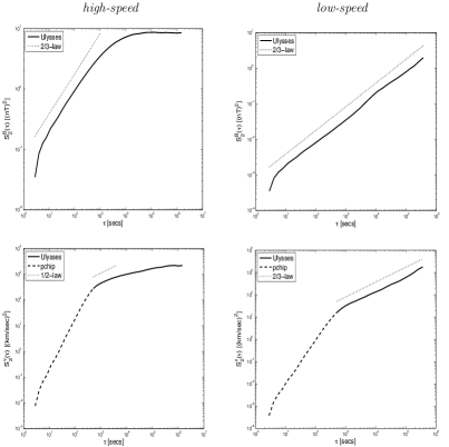
Figure 2: Second-Order Structure Functions. Top Panels: Magnetic structure functions. The solid line plots the Ulysses data, the dotted line is a 2/3 power law. Bottom Panels: Velocity structure functions. The solid line is again the raw data. The dotted line for the high-speed case on the left is a 1/2 power, while the dotted line for the low-speed case on the right is a 2/3 power. The dashed lines are the results below 4 mins resulting from the pchip interpolation of the velocity field.

We next present results for the second-order structure-functions of time increments

$$S_{2}^{X}(\tau)=\overline{|{\textit{{X}}}(t+\tau)-{\textit{{X}}}(t)|^{2}}$$ (5.5)

with ${\textit{{X}}}={\textit{{B}}},{\textit{{u}}}$ and overline $\overline{()}$ denoting time-average over the entire interval of data. For the purposes of later evaluation of the slip velocity via formula (5.1) we interpolate the 4 min plasma velocity data to the 1 sec grid of the magnetic data using piece-wise cubic Hermite interpolating polynomials (pchip). Although there is no physical significance of the interpolated velocity data at times less than 4 min, we plot their structure functions down to 1 sec time separations in order to show the effects of the  interpolation. The structure functions plotted in Figure 2 show the typical features of high-speed and low-speed solar wind around 1 AU. The low-speed solar wind exhibits a Kolmogorov-type 2/3 power-law scaling for both magnetic and velocity fields over the entire range of available times,  consistent with the theory of Goldreich & Sridhar (1995). The magnetic field data begin to bend over to a steeper scaling at $\tau$ a few seconds, around the ion gyro-period.   The velocity field structure function if accurately measured to 1 sec resolution would presumably have similar behavior, but the interpolated data lead to a steeper decay with a power of 2 due to the smooth polynomial. The high-speed wind structure functions are quite similar to those for the low-speed solar wind at times less than about $10^{4}$ sec. The primary difference in that range is that the scaling exponent for the velocity structure function appears closer to 1/2 than 2/3, as often observed in the high-speed wind near 1 AU (Podesta et al., 2007), although the precise determination here is impossible since only about a decade exists between 4 minutes and the outer time, which is somewhat less than $10^{4}$ sec. The main difference between high-speed and low-speed wind appears above that outer time, where the high-speed wind shows a flattening of both the magnetic and the velocity structure functions. This corresponds to the so-called “1/f range” of scales (Matthaeus & Goldstein, 1986), which is believed to be largely a mixture of a noninteracting, antialigned population of Alfvén waves and magnetic force-free structures ejected from the sun (Wicks et al., 2013a, b). Hereafter we discuss the low- and high-speed cases separately.

5.1.1 Low-Speed Case

We first plot the time series for the magnetic and velocity fields in the slow-speed case. See Fig. 3. From examination of the data for tangential component of the magnetic field, one can see that there are sector crossings during day 152, late on day 153 and a major crossing during the whole of day 157. The last is an example of a complex, broadened heliospheric current sheet (HCR), of the type which has been shown to occur with increasing likelihood at greater distances from the sun and under conditions of solar maximum (Roberts et al., 2005). Note that, not only does the tangential component of the magnetic field undergo a large reversal in sign on day 157, but also the other two components reverse sign. Fig. 4, which plots other plasma properties, shows additional signatures of the HCS on day 157, such as sizable increases in density and temperature and different levels of magnetic field strength be-

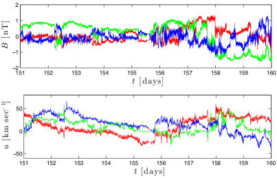
Figure 3: Magnetic and Velocity Components of Slow Wind Time-Series. The upper panel plots the magnetic field components and the lower panel velocity field components. The red line represents radial component, green tangential, and blue normal, in the standard RTN coordinate system. The plotted radial component of the velocity is the fluctuation field $u_{R}^{\prime}=u_{R}-\bar{u}_{R},$ with the average value $\bar{u}_{R}=$769 km ${\rm sec}^{-1}$ subtracted.

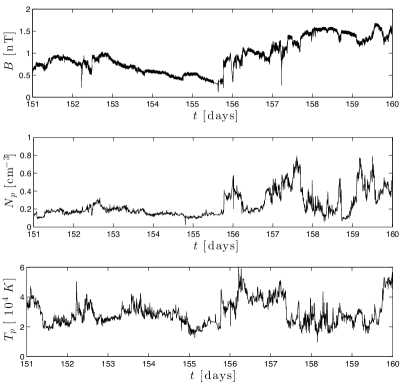
Figure 4: Field Strength, Density and Temperature of Slow Wind Time-Series. Upper panel: field strength, middle panel: density, and bottom panel: temperature.

fore and after the transition.

A close examination of the tangential velocity components in Fig. 3 shows also apparent veloc-

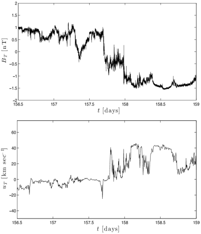
Figure 5: Tangential Magnetic Field and Velocity at Broad Heliospheric Current Sheet. Upper panel: tangential component of magnetic field. Lower panel: the tangential component of plasma velocity.

ity jets associated with each of the three sector crossings, in particular at the HCS. To examine the latter more carefully, we show a closer view of the tangential components of magnetic and velocity fields across the HCS in Fig. 5. The reversal of the tangential component of the magnetic field is particularly broad, extending over days 157-158.5. The associated exhaust is a bit narrower, covering days 157.75-158.75. Notice that the speed of this broad outflow is about 40 km ${\rm sec}^{-1}$, just a bit less than the local upstream Alfvén speeds. This seems to be a likely example of Lazarian & Vishniac (1999) turbulent reconnection, associated to the embedding of the HCS in a strongly turbulent environment. Notice that the observed value of $B_{rms}/\bar{B}$ away from the HCS itself is about 0.5. Furthermore, the plasma fluid within the HCS is itself strongly turbulent, as required by the Lazarian & Vishniac (1999) theory. Fig. 6 plots the structure function of the magnetic field inside the HCS, averaging over days 157-158.5. There is a

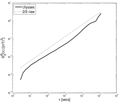
Figure 6: Magnetic Structure Function inside the Broad Heliospheric Current Sheet. Same as in Fig.2, top right panel, but defined by an average only over days 157-158.5 inside the HCS.

clear 2/3-law scaling, covering about 4 decades from $10-10^{5}$ secs. Finally, we note that our coarse-graining analysis in section 4.2 shows that at the length-scales of this event, of order an AU, all microscopic plasma non-idealities are completely irrelevant. Turbulent reconnection seems to be the only plausible explanation.

We next turn to the evaluation of the formula (5.1) for the turbulent slip velocity. Since the full three-dimensional data is unavailable to perform low-pass filtering, we follow standard practice in experimental turbulence studies (e.g. Bruno & Carbone (2013), Section 7; Stolovitzky et al. (1998)) and use filtering on the time axis as a one-dimensional surrogate. To carry out the required coarse-graining, we apply a box-filter to the observational time series, with the filter half-width identified with coarse-graining time-scale $\tau.$ As discussed earlier, we use pchip interpolation of the velocity to define the pointwise cross product ${\textit{{u}}}\hbox{\boldmath$\times$}{\textit{{B}}}.$ We plot in Fig. 7 the instantaneous turbulent drift velocities for the filter half-width $\tau=$2 days. It is immediately obvious that there is a large tangential component of the drift velocity associated with the HCS, from day 156-158, with a maximum slip speed of nearly 40 km ${\rm sec}^{-1}$. The plots for other choices of half-width $\tau$ (not shown) are  similar,  as long as $\tau$ is greater than  1 day.

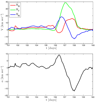
Figure 7: Turbulent Drift Velocity and Alpha Parameter for Low-Speed Time-Series. Top panel: drift velocity for filter half-width $\tau=2$ days. The color scheme is as in Fig.3. Bottom panel: the $\alpha$ parameter for the same half-width $\tau=2$ days.

The peak tangential drift velocity increases with $\tau$ over the range that we can study, with peak values of $v_{{\rm slip},T}^{{\max}}=$2.21, 14.9, 29.0, and 38.6 km ${\rm sec}^{-1}$, for $\tau=$0.5, 1.0, 1.5, 2.0 days, respectively. There is no observable “jet” of tangential slip velocity at the HCS for $\tau=0.5,$ but the “jet” exists and becomes broader for increasing $\tau\geq 1.$ As remarked at the end of section 4, the net velocity of the field lines is in fact the sum of the resolved plasma velocity and the drift velocity at that scale. These total tangential speeds of magnetic field-lines are even a bit larger, with maximum values in the HCS of $\bar{u}_{T}+v_{{\rm slip},T}=$28.6, 18.9, 34.8, and 44.0 km ${\rm sec}^{-1}$, for $\tau=$0.5, 1.0, 1.5, 2.0 days, respectively.

The most important observation is that the largest component of the slip velocity is the tangential component, which has a positive sign. With the standard definition of RTN coordinates, this slip velocity is in the direction of the solar rotation. Hence, this slippage will tend to make

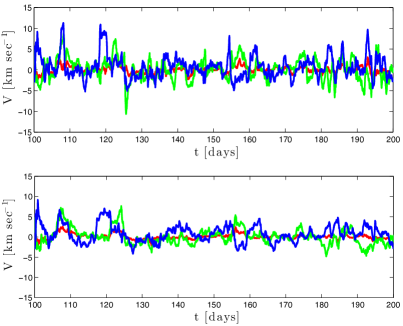
Figure 8: Turbulent Drift Velocity for High-Speed Time-Series at Two Scales. Upper panel: components of turbulent drift velocities for filter half-width $\tau=1$ day. Lower panel: components of drift velocity for half-width $\tau=2$ days. The color scheme is as in Fig.3.

the field-lines less frozen into the plasma fluid and rotate more with the sun, so that the spiral will become less tightly wound. This is in qualitative agreement with the observations of Burlaga et al. (1982) and Khabarova & Obridko (2012). For consistency, we should check that the $\alpha$ parameter is small relative to the drift velocity. As can be seen from Fig. 7, this is marginally true, with $\alpha\sim(1/3)v_{{\rm slip}}$ for $\tau=2$ days. The fact that the $\alpha$ parameter is not completely negligible suggests that there is some magnetic dynamo action/inverse cascade of magnetic helicity in the HCS. We should note also that the tangential drift velocity is positive away from the HCS (except briefly at the end of day 155) and takes on typical values of about 1 km ${\rm sec}^{-1}$. The minor sector crossings on days 152 and 153 presumably contribute to such drifts. Such background turbulent slippage will also contribute to the observed deviations from the Parker spiral model.

5.1.2 High-Speed Case

The situation for the high-speed wind case is quite different. We plot in Fig. 8 the turbulent

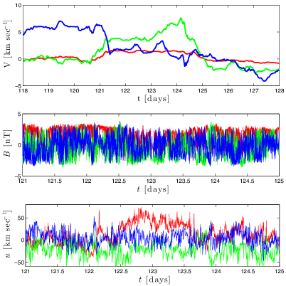
Figure 9: Close-up View of High-Speed Wind Data for Large Tangential Drift Region. Top panel: turbulent drift velocities for filter half-width $\tau=2$ days over the smaller interval of days 118-128. Middle panel: components of magnetic field for days 121-125. Bottom panel: components of velocity field for days 121-125. The color scheme for all panels is as in Fig.3, and as there the plotted radial component in the bottom panel is $u_{R}^{\prime},$ the fluctuation field.

slip velocities over the entire 100 days, for the two filter half-widths $\tau=1$ day and $\tau=2$ days. The first observation is that the peak values are only about 10 km ${\rm sec}^{-1}$, one-quarter of the peak for the slow wind case. Second, the largest component is the normal component, not the tangential. Finally, the peak magnitudes decrease going from $\tau=1$ day to $\tau=2$ days, unlike for the slow-wind case where there was a sizable increase. There is in fact a slight increase in the mean values over the whole interval, with $[\bar{v}_{R},\bar{v}_{T},\bar{v}_{N}]=[0.0639,\ 0.0878,\ 0.6360]$ km ${\rm sec}^{-1}$ for $\tau=1$ day, but $[\bar{v}_{R},\bar{v}_{T},\bar{v}_{N}]=[0.0981,\ 0.0782,\ 0.7841]$ for $\tau=2$ days. However, the extreme values are clearly decreased.

There are at least two plausible explanations for this decrease. One reason may be the strong alignment of $\delta{\textit{{B}}}(\hbox{\boldmath$\ell$})$ and $\delta{\textit{{u}}}(\hbox{\boldmath$\ell$})$ in the “1/f-range” of the high-speed wind, which leads to a large depletion of the slip velocity when $\ell$ increases in that range. Note indeed that Wicks et al. (2013a, b) find the non-aligned, nonlinearly cascading modes in the “1/f-range” have about an order of magnitude smaller energy than the aligned, non-interacting modes. The second reason has to do with the atypicality of very large-scale reconnection events of conventional type in the high-speed wind (Gosling, 2007). In the entire 100 days of high-speed data, we see no AU-scale events of the type which occurred in the low-speed wind at the HCS. If we focus on the regions of peak tangential drift velocity in the high-speed wind, we see a very different structure. Fig. 9 zooms in on such a peak around day 123 for $\tau=$ 2 days. As can be seen, the magnetic field components appear to the eye rather structureless and stochastic. On the other hand, there is clear structure in the velocity field, with the radial velocity fluctuation $u_{R}^{\prime}$ around the mean value 769 km ${\rm sec}^{-1}$ increased over a 1-day interval around day 123. The peak in the slip velocity at this point appears to result therefore from the interaction between two extensive high-speed streams, with radial velocities differing by about 50 km ${\rm sec}^{-1}$, and not from any large-scale magnetic structure.

5.1.3 Discussion

Our purpose in this section was to use observational data on the solar wind to make a first estimate of the size, directionality, and origin of turbulent slip velocities in that environment. These effects appear promising to explain the observed deviations from the Parker spiral in the inner heliosphere, but to do so quantitatively will require more extensive studies. We hope to carry these out in the near future. Several open issues remain to be clarified, such as the relative importance in the slow wind of background turbulence drift and of the larger turbulent slips at the HCS. The accuracy of one-dimensional surrogates of three-dimensional filtering should be investigated in numerical simulations of MHD turbulence, etc. On the other hand, this theory already accounts naturally for the smaller deviations from the spiral model observed in the high-speed solar wind than in low-speed, and in solar minimum conditions than in solar maximum. The peak values of slip velocity in the slow wind at solar maximum are about 10% of the mean plasma velocity, whereas for the high-speed wind at solar minimum they are only about 1% (and even less in the tangential direction). Furthermore, our coarse-graining analysis of the Generalized Ohm’s Law in section 4.2 implies that, for the very long-time averages employed by Burlaga et al. (1982) and Khabarova & Obridko (2012), alternative microscopic plasma mechanisms of line-slippage are irrelevant and cannot explain the observed deviations.

5.2 Other Large-Scale Heliospheric Reconnection

In addition to the breakdown of the Parker model considered above, another type of deviation has been documented in daily averages of Voyager 1 observations in the heliosheath between 2007-2011, when the spacecraft was about 110 AU from the Sun (Richardson et al., 2013). At this distance, the Parker model predicts that the magnetic field is almost entirely tangential, $B=B_{T},$ and magnetic flux conservation implies that $u_{R}BR$ should be constant in $R$ (Parker, 1963). Richardson et al. (2013) interpreted their observations of a “flux deficit” in terms of kinetic-scale magnetic reconnection, due to ion-scale current sheets created by compression of magnetic sectors in the heliosheath. However, these observations may also be explained by magnetic reconnection in the heliosheath due to MHD turbulence, as earlier suggested by Lazarian & Opher (2009). This would lead to reconnection when the sector widths were still much greater than required by kinetic mechanisms. Note that there is direct evidence for MHD-like turbulence with a -5/3 energy spectrum of magnetic fluctuations in the sectored region of the heliosheath, from Voyager 1 data in the year 2009 (Burlaga & Ness (2010), Figure 8), within the time period where reconnection appears to occur.

Finally, many magnetic reconnection events of conventional nature have been apparently directly observed in the solar wind at solar distances around 1 AU, as documented in a recent review of Gosling (2012). These are more extreme events than background, gradual slippage and involve a sizable release of magnetic energy. Small-scale current sheets with widths of order the ion inertial length that exhibit observable reconnection usually have exhausts at most a few hundred times wider and frequently have small shear angles/strong guide fields (Gosling et al., 2007; Gosling & Szabo, 2008). However, there is also a sizable number of very large-scale reconnection events in the solar wind, some of them associated with interplanetary coronal mass ejections and magnetic clouds or occasionally magnetic disconnection events at the heliospheric current sheet (Phan et al., 2009; Gosling, 2012). These events have reconnection outflows with widths up to nearly $10^{5}$ ion inertial lengths and appear to be in a prolonged, quasi-stationary regime with reconnection lasting for several hours. Gosling interprets these events in terms of the Petschek (1964) reconnection model although, as he points out himself, there are observations not in strict agreement with that model. This interpretation is also theoretically puzzling since numerical studies (Biskamp, 1986; Uzdensky & Kulsrud, 2000) have shown that Petschek reconnection is not sustainable in laminar, MHD flows, but relaxes to the slow Sweet-Parker type. The belief that these events are Petschek-like seems to rest on the fact that the Hall and electron inertia effects can stabilize such X-type reconnection in ion-scale geometries (Shay et al., 1998).

The scale of the apparent reconnection events documented by Gosling (2012) is so great, however, that they will still appear to be reconnection even if coarse-grained on inertial-range scales $\ell$ much greater than the ion gyroradius $\rho_{i}.$ At those scales, our analysis implies that microscopic non-ideal terms from Hall field and electron inertia are irrelevant. Such large-scale reconnection events must be due to the ideal turbulence effects in the solar wind environment rather than to plasma non-ideality. In fact, these events appear to be very promising candidates for turbulent reconnection as in the Lazarian & Vishniac (1999) theory. It should be noted that the events observed by Gosling often show substantially increased proton densities in the exhausts, as well as enhancements of magnetic field strength and proton temperature, effects also seen in the HCS event analyzed in section 5.1.1. Whereas the coarse-graining method employed in section 4 assumed constant density, the more general analysis carried out in Appendix A is able to describe such effects.

In any case, the discussion of the slip-source in section 3, which does not assume incompressibility, already makes it clear that reconnection in the most general sense must occur ubiquitously throughout the turbulent solar-wind.

Appendix A Density Variations

Previously we ignored variations of density in our discussion of the Generalized Ohm’s Law. This would be a serious omission for the solar wind, where the observations of apparent reconnection events by Gosling and colleagues (Gosling, 2012) show frequently sizable enhancements of density and proton temperature in the outflows. The interpretation of Gosling for these events is that they are Petschek (1964) reconnection with the outflows bounded by slow-mode shocks. In addition to these density variations during reconnection, there are also known to be turbulent fluctuations of plasma density in the solar wind. A paper of Bellamy et al. (2005) contains recent observations at solar distances 1-60 AU and a good review of previous studies. The spectrum of turbulent density fluctuations has two power-law ranges, a low-wavenumber part with a $k^{-2}$ spectrum and a high-wavenumber part with a $k^{-5/3}$ spectrum. Bellamy et al. (2005) interpret the $k^{-2}$ spectrum as due to abrupt discontinuities on the time-scales of a few hours and up, which are left over by their data selection procedure, which removes obvious shocks. The high-wavenumber $k^{-5/3}$ spectrum of density fluctuations is in roughly the same range of wavenumbers as the similar inertial-range spectrum of magnetic fluctuations. A popular interpretation is that it is a passive scalar cascade of slow magnetosonic modes driven by the nonlinear cascade of shear-Alfvén modes (Schekochihin et al., 2009). There is evidence from observations that density fluctuations in the solar wind consist mainly of slow-modes with possibly a tiny admixture of fast modes (Howes et al., 2012).

As we show now, the extension of our analysis of the Generalized Ohm’s Law carries over easily to plasma flows with arbitrarily large variations of density (including shocks). The simplest way to do so is to make use of the density-weighted, spatial-coarse-graining Favre average (Favre, 1969), which is defined by the formula

$$\tilde{f}_{\ell}=\frac{1}{\bar{n}_{\ell}}\overline{(nf)_{\ell}}.$$ (A1)

With this density-weighted averaging operation, it is straightforward to obtain the coarse-grained form of the Generalized Ohm’s Law to be

$$\tilde{{\textit{{E}}}}_{\ell}+\frac{1}{c}\tilde{{\textit{{u}}}}_{\ell}\hbox{\boldmath$\times$}\tilde{{\textit{{B}}}}_{\ell}=-\tilde{\hbox{\boldmath${\mathit{\varepsilon}}$}}_{\ell}+\widetilde{\left(\eta{\textit{{J}}}\right)_{\ell}}+\frac{1}{\bar{n}_{\ell}ec}\overline{({\textit{{J}}}\hbox{\boldmath$\times$}{\textit{{B}}})_{\ell}}-\frac{1}{\bar{n}_{\ell}}\hbox{\boldmath${\mathit{\nabla}}$}\hbox{\boldmath$\cdot$}{\overline{\textbf{P}}}_{e,\ell}+\frac{m_{e}}{\bar{n}_{\ell}e^{2}}\left[\frac{\partial\bar{{\textit{{J}}}}_{\ell}}{\partial t}+\hbox{\boldmath${\mathit{\nabla}}$}\hbox{\boldmath$\cdot$}\overline{\left({\textit{{J}}}{\textit{{u}}}+{\textit{{u}}}{\textit{{J}}}-\frac{1}{ne}{\textit{{J}}}{\textit{{J}}}\right)_{\ell}}\right],$$ (A2)

where the turbulent electric field is now given by

$$\tilde{\hbox{\boldmath${\mathit{\varepsilon}}$}}_{\ell}=-\frac{1}{c}\left[\widetilde{({\textit{{u}}}\hbox{\boldmath$\times$}{\textit{{B}}})_{\ell}}-\tilde{{\textit{{u}}}}_{\ell}\hbox{\boldmath$\times$}\tilde{{\textit{{B}}}}_{\ell}\right],$$ (A3)

the Favre-average 2nd-order cumulant.

The first and most important observation is that, other than the Ohmic contribution, all of the non-ideal terms in the coarse-grained Generalized Ohm’s Law are identical to those obtained in section 4.2, except that they are multiplied by $1/\bar{n}_{\ell}$ rather than $1/n.$ The only difference to the old estimates is thus that they are multiplied by an additional factor

$$\frac{n}{\bar{n}_{\ell}}=1-\frac{1}{\bar{n}_{\ell}}\int d^{3}r\ G_{\ell}({\textit{{r}}})\delta n({\textit{{r}}}).$$ (A4)

This is generally $\approx 1$ and is an order unity factor even in the presence of shocks in the density. Here is a good point to observe that all of our conclusions in section 4.2 remain valid in the presence of shocks. We generally assumed K41 scaling $\delta{\textit{{B}}}({\textit{{r}}})\sim r_{\perp}^{1/3},$ $\delta n({\textit{{r}}})\sim r^{1/3}$ or something similar, but at shock points these increments become nearly independent of the separation vector magnitude $r,$ until $r$ falls below the width of the shock. However, all of our estimates are pointwise in space position x and, even at points where increments are independent of $r,$ we always have extra factors of $\delta_{e}/\ell$ to make the coarse-grained non-ideal terms small for $\ell\gg\delta_{e}.$

Another observation is that the Favre-averaged quantities $\tilde{{\textit{{E}}}}_{\ell},\tilde{{\textit{{u}}}}_{\ell},\tilde{{\textit{{B}}}}_{\ell},$ and $\tilde{\hbox{\boldmath${\mathit{\varepsilon}}$}}_{\ell}$ are rather close in value to the ordinary coarse-grained quantities $\bar{{\textit{{E}}}}_{\ell},\bar{{\textit{{u}}}}_{\ell},\bar{{\textit{{B}}}}_{\ell}$ and $\hbox{\boldmath${\mathit{\varepsilon}}$}_{\ell}$. This can be seen from simple identities (Aluie, 2013), for the Favre average

$$\tilde{f}=\bar{f}+\frac{1}{\bar{n}}\tau(n,f)=\bar{f}+\frac{1}{\bar{n}}O\left(\delta n\ \delta f\right)$$ (A5)

and for the Favre-average 2nd-cumulant $\tilde{\tau}(f,g)=\widetilde{fg}-\tilde{f}\tilde{g},$

$$\tilde{\tau}(f,g) = \tau(f,g)+\frac{1}{\bar{n}}\tau(n,f,g)-\frac{1}{\bar{n}^{2}}\tau(n,f)\tau(n,g)$$ (A6)

$$= \tau(f,g)+\frac{1}{\bar{n}}O\left(\delta n\ \delta f\ \delta g\right)+\frac{1}{\bar{n}^{2}}O\left((\delta n)^{2}\ \delta f\ \delta g\right).$$ (A7)

For the order-of-magnitude estimates, see Appendix B. The first identity (A5) yields

$$\tilde{{\textit{{B}}}}_{\ell}=\bar{{\textit{{B}}}}_{\ell}\left[1+O\left(\delta n(\ell)\ \delta B(\ell)\right)\right]\simeq\bar{{\textit{{B}}}}_{\ell}\left[1+O\left(\frac{\ell}{L}\right)^{2/3}\right],$$ (A8)

where the final estimate holds at typical points with K41 scaling of the increments and where $L$ is the outer scale of the inertial range. Exactly similar results hold for $\tilde{{\textit{{u}}}}_{\ell}$ and $\tilde{{\textit{{E}}}}_{\ell}$ by the same argument. For the turbulent electric field one can likewise infer from (A7) that

$$\tilde{\hbox{\boldmath${\mathit{\varepsilon}}$}}_{\ell}=\hbox{\boldmath${\mathit{\varepsilon}}$}_{\ell}\left[1+O\left(\frac{\delta n(\ell)}{\bar{n}_{\ell}}\right)\right]\simeq\hbox{\boldmath${\mathit{\varepsilon}}$}_{\ell}\left[1+O\left(\frac{\ell}{L}\right)^{1/3}\right],$$ (A9)

with the final estimate holding again at typical points. We see that the Favre coarse-grained and ordinary coarse-grained quantities are very similar when density variations are small relative to the mean, and of similar orders of magnitude when density variations are large (e.g. at shocks).

The most troublesome term is, in fact, the Favre-averaged Ohmic electric field. Although the current is a total space-derivative, because of Ampere’s law ${\textit{{J}}}=(c/4\pi)\hbox{\boldmath${\mathit{\nabla}}$}\hbox{\boldmath$\times$}{\textit{{B}}},$ the same is not true of the product of density and current, $n{\textit{{J}}}.$ Thus, unlike before, coarse-graining this product to obtain the Favre-average of the Ohmic electric field does not yield any powers of $\ell^{-1}$, which would make it irrelevant for increasing $\ell.$ Additional complicating x-dependences to the Ohmic electric field arise from the fact that resistivity is a tensor $\hbox{\boldmath$\eta$}=\frac{1}{\sigma_{\|}}\hat{{\textit{{B}}}}\hat{{\textit{{B}}}}+\frac{1}{\sigma_{\perp}}\left({\textbf{I}}-\hat{{\textit{{B}}}}\hat{{\textit{{B}}}}\right)$ with a position-dependent director field $\hat{{\textit{{B}}}}({\textit{{x}}}).$ Furthermore, the collisional conductivities $\sigma_{\perp},\sigma_{\|}$ have very weak (logarithmic) dependence on density but strong dependence $\propto[T_{e}({\textit{{x}}})]^{3/2}$ on the electron temperature. Luckily, the Ohmic electric field is tiny in the solar wind, even without coarse-graining. Using $\sigma\sim e^{2}n\tau_{e,i}/m_{e}$, with $\tau_{e,i}$ the electron collision time with ions, $\lambda_{mfp,e}=v_{th,e}\tau_{e,i}$ the electron mean-free path, and $J\sim c\delta B(\delta_{e})/4\pi\delta_{e},$ one finds easily

$$\eta J\sim\left(\frac{\delta_{e}}{\lambda_{mfp,e}}\right)\cdot\frac{1}{c}v_{th,e}\delta B(\delta_{e}).$$ (A10)

Since the ratio $\delta_{e}/\lambda_{mfp,e}$ is $10^{-8}$ or smaller in the solar wind, the Ohmic electric field can be neglected even without coarse-graining.

Appendix B Mathematical Identities for Coarse-Graining Cumulants

Suppose that $\{f_{i}|i=1,2,3\cdots\}$ are any set of space fields. Note that

$$\overline{(f_{i_{1}}\ldots f_{i_{p}})}_{\ell}({\textit{{x}}}) = \int d^{d}r\,\,G_{\ell}({\textit{{r}}})f_{i_{1}}({\textit{{x}}}+{\textit{{r}}})\ldots f_{i_{p}}({\textit{{x}}}+{\textit{{r}}})$$

$$= \langle(\sigma f_{i_{1}})\ldots(\sigma f_{i_{p}})\rangle_{\ell}({\textit{{x}}})$$

where $G$ is any smooth, rapidly decaying, positive function with space integral unity, and

$$(\sigma f_{i})({\textit{{x}}})=f_{i}({\textit{{x}}}+{\textit{{r}}})$$ (B1)

is the shift operator and $\langle\cdot\rangle_{\ell}$ denotes average over the displacement vector r with density $G_{\ell}({\textit{{r}}}).$ We thus see that $\overline{f_{i_{1}}\ldots f_{i_{p}}}$ is a correlation function of the “random variables” $\sigma f_{i_{1}}$,…,$\sigma f_{i_{p}}$. (In this formula and the following we omit for simplicity of notations any explicit reference to the coarse-graining length $\ell.$) The cumulants of the variables $f_{1}({\textit{{x}}}+{\textit{{r}}}),\ldots,f_{n}({\textit{{x}}}+{\textit{{r}}})$ for space-averaging with respect to the density $G_{\ell}({\textit{{r}}})$ on r, denoted by

$$\tau(f_{i_{1}},\ldots,f_{i_{p}})=\langle(\sigma f_{i_{1}})\ldots(\sigma f_{i_{p}})\rangle^{c},$$ (B2)

are defined as follows:

$$\bar{f}_{1} = \tau(f_{1})$$

$$\overline{f_{1}f_{2}} = \tau(f_{1},f_{2})+\bar{f}_{1}\bar{f}_{2}$$

$$\overline{f_{1}f_{2}f_{3}} = \tau(f_{1},f_{2},f_{3})+\bar{f}_{1}\tau(f_{2},f_{3})+\bar{f}_{2}\tau(f_{1},f_{3})+\bar{f}_{3}\tau(f_{1},f_{2})+\bar{f}_{1}\bar{f}_{2}\bar{f}_{3}$$

and, iteratively,

$$\overline{f_{1}\ldots f_{n}}=\sum_{I\in\mathcal{P}}\prod^{p}_{j=1}\tau(f_{i_{1}^{(j)}},\ldots,f_{i_{n_{j}}^{(j)}})$$ (B3)

where the sum is over the set $\mathcal{P}$ of all partitions $I=\{i^{(1)}_{1},\ldots,i^{(1)}_{n_{1}}\},\ldots,\{i^{(p)}_{1},\ldots,i^{(p)}_{n_{p}}\}$ of the set $\{1,2,...,n\}$ with $\sum^{p}_{j=1}n_{j}=n$. We thus see that

$$\overline{f_{1}\ldots f_{n}}=\tau(f_{1},\ldots,f_{n})+\mbox{terms defined by lower-order cumulant functions}$$ (B4)

so that one may solve successively to obtain

$$\tau(f_{1}) = \bar{f}_{1},\,\,\,\,\,\,\,\,\,\,\,\,\tau(f_{1},f_{2})=\overline{f_{1}f_{2}}-\bar{f}_{1}\bar{f}_{2},$$

$$\tau(f_{1},f_{2},f_{3}) = \overline{f_{1}f_{2}f_{3}}-\bar{f}_{1}\overline{f_{2}f_{3}}-\bar{f}_{2}\overline{f_{1}f_{3}}-\bar{f}_{3}\overline{f_{1}f_{2}}+2\bar{f}_{1}\bar{f}_{2}\bar{f}_{3},\,\,\,\,{\rm etc.}$$

These cumulants are called “generalized central moments” in fluid turbulence literature (Germano, 1992) and “connected correlation functions” in statistical physics and quantum field theory (Huang, 1987).

A very important fact is that the cumulants of the shift fields can be re-expressed as cumulants of the difference fields:

$$\delta_{\textit{{r}}}f_{i}({\textit{{x}}})=\sigma_{\textit{{r}}}f_{i}({\textit{{x}}})-f_{i}({\textit{{x}}}).$$ (B5)

The precise statement is as follows:

Proposition 1

The connected correlation functions of $\delta f_{i}$ and $\sigma f_{i}$ are related for $p=1$ by

$$\tau(f_{i})=\bar{f}_{i}=f_{i}+\langle\delta f_{i}\rangle.$$ (B6)

and for $p>1$ are equal

$$\tau(f_{i_{1}},\cdots,f_{i_{p}})=\,\,\langle\delta f_{i_{1}}\ldots\delta f_{i_{p}}\rangle^{c}$$ (B7)

Concrete examples are for $p=2$

$$\tau(f_{i},f_{j})=\langle\delta f_{i}\delta f_{j}\rangle-\langle\delta f_{i}\rangle\langle\delta f_{j}\rangle,$$ (B8)

and for $p=3$

$$\tau(f_{i},f_{j},f_{k})\,\, = \,\,\langle\delta f_{i}\delta f_{j}\delta f_{k}\rangle-\langle\delta f_{i}\delta f_{j}\rangle\langle\delta f_{k}\rangle$$

$$-\langle\delta f_{i}\delta f_{k}\rangle\langle\delta f_{j}\rangle-\langle\delta f_{j}\delta f_{k}\rangle\langle\delta f_{i}\rangle\ +2\langle\delta f_{i}\rangle\langle\delta f_{j}\rangle\langle\delta f_{k}\rangle.$$

Constantin et al. (1994) gave a concise proof of Onsager’s theorem on dissipative anomaly for turbulent Euler solutions using the formula for $p=2$, which our proposition generalizes to all $p$-th order cumulants. The result follows from the shift invariance of the cumulants, that is, the fact that the cumulants of the “random” variables $\sigma_{\textit{{r}}}f_{i}({\textit{{x}}})=f_{i}({\textit{{x}}}+{\textit{{r}}})$ do not change under a “non-random” (i.e. r-independent) shift by $-f_{i}({\textit{{x}}}).$ Because this property plays a fundamental role in our calculations we give, for completeness, a standard proof using a method of generating functions.

The generating function for correlation functions of shifted fields is

$$Z^{\sigma}(\hbox{\boldmath${\mathit{\alpha}}$})\,=\,\langle\exp(\sum_{i\in I}\alpha_{i}\,\sigma f_{i})\rangle.$$ (B9)

In fact, it is easy to check that

$$\overline{(f_{i_{1}}\ldots f_{i_{p}})}=\frac{\partial^{p}}{\partial\alpha_{i_{1}}\ldots\partial\alpha_{i_{p}}}Z^{\sigma}(\hbox{\boldmath${\mathit{\alpha}}$})|_{\hbox{\boldmath${\mathit{\alpha}}$}={\textbf{0}}}$$ (B10)

The cumulants are generated by the logarithm of that function $W^{\sigma}(\hbox{\boldmath${\mathit{\alpha}}$})=\ln Z^{\sigma}(\hbox{\boldmath${\mathit{\alpha}}$}),$ i.e.

$$\tau(f_{i_{1}}\ldots f_{i_{p}})=\frac{\partial^{p}}{\partial\alpha_{i_{1}}\ldots\partial\alpha_{i_{p}}}W^{\sigma}(\hbox{\boldmath${\mathit{\alpha}}$})|_{\hbox{\boldmath${\mathit{\alpha}}$}={\textbf{0}}}.$$ (B11)

This is the so-called linked cluster-theorem. See Huang (1987), section 10.1. The correlation functions of the increments $\langle\delta f_{i_{1}}\ldots\delta f_{i_{p}}\rangle$ are likewise generated by the function

$$Z^{\delta}(\hbox{\boldmath${\mathit{\alpha}}$})\,=\,\langle\exp(\sum_{i\in I}\alpha_{i}\,\delta f_{i})\rangle,$$ (B12)

and the connected correlation functions by the function $W^{\delta}(\hbox{\boldmath${\mathit{\alpha}}$})=\ln Z^{\delta}(\hbox{\boldmath${\mathit{\alpha}}$}),$ i.e.

$$\langle(\delta f_{i_{1}})\ldots(\delta f_{i_{p}})\rangle^{c}=\frac{\partial^{p}}{\partial\alpha_{i_{1}}\ldots\partial\alpha_{i_{p}}}W^{\delta}(\hbox{\boldmath${\mathit{\alpha}}$})|_{\hbox{\boldmath${\mathit{\alpha}}$}={\textbf{0}}},$$ (B13)

again by the linked-cluster theorem. Now comes the key observation: since $f_{i}({\textit{{x}}})$ does not depend on r, it can be taken outside the average $\langle.\rangle$. Thus, using $\delta f_{i}=\sigma f_{i}-f_{i}$,

$$Z^{\delta}(\hbox{\boldmath${\mathit{\alpha}}$})\, = \,\langle\exp(\sum_{i\in I}\alpha_{i}\,\delta f_{i})\rangle,=\langle\exp(\sum_{i\in I}\alpha_{i}\,\sigma f_{i})\rangle\exp(-\sum_{i\in I}\alpha_{i}f_{i})=Z^{\sigma}(\hbox{\boldmath${\mathit{\alpha}}$})\exp(-\sum_{i\in I}\alpha_{i}f_{i})$$

Taking the logarithm of both sides then gives

$$W^{\delta}(\hbox{\boldmath${\mathit{\alpha}}$})=W^{\sigma}(\hbox{\boldmath${\mathit{\alpha}}$})-\sum_{i\in I}\alpha_{i}f_{i}$$ (B14)

The Proposition 1 then follows by multiple differentiations with respect to $\hbox{\boldmath${\mathit{\alpha}}$}.$

A further property of the cumulants implied by their shift-invariance is a simple transformation law under space-translations. We illustrate this property by the following expression for the space-translated 2nd-order cumulant:

$$\tau(f_{i},f_{j})({\textit{{x}}}+{\textit{{{a}}}},t) = \int d^{d}r\,\,G_{{\textit{{{a}}}},\ell}({\textit{{r}}})\delta f_{i}({\textit{{r}}},t)\delta f_{j}({\textit{{r}}},t)$$ (B16)

$$\,\,\,\,\,\,\,\,-\int d^{d}r\,\,G_{{\textit{{{a}}}},\ell}({\textit{{r}}})\delta f_{i}({\textit{{r}}},t)\int d^{d}r^{\prime}G_{{\textit{{{a}}}},\ell}(r^{\prime})\delta f_{j}({\textit{{r}}}^{\prime},t)$$

with kernel $G_{{\textit{{{a}}}},\ell}$ centered at point ${\textit{{{a}}}}:$

$$G_{{\textit{{{a}}}},\ell}({\textit{{r}}})=\ell^{-d}G(\frac{{\textit{{r}}}-{\textit{{{a}}}}}{\ell}).$$ (B17)

The general fact is that such expressions for translated cumulants are identical to the corresponding expressions for untranslated cumulants in terms of increments, except that the average with respect to $G_{\ell}$ is replaced by average with respect to $G_{{\textit{{{a}}}},\ell}.$ To establish this fact, first note

$$\tau(f_{i},f_{j})({\textit{{x}}}+{\textit{{{a}}}})=\int d^{d}r\,\,G_{\ell}({\textit{{r}}})[f_{i}({\textit{{x}}}+{\textit{{{a}}}}+{\textit{{r}}})-f_{i}({\textit{{x}}}+{\textit{{{a}}}})][f_{j}({\textit{{x}}}+{\textit{{{a}}}}+{\textit{{r}}})-f_{j}({\textit{{x}}}+{\textit{{{a}}}})]$$

$$-\int d^{d}r\,\,G_{\ell}({\textit{{r}}})[f_{i}({\textit{{x}}}+{\textit{{{a}}}}+{\textit{{r}}})-f_{i}({\textit{{x}}}+{\textit{{{a}}}})]\int d^{d}r^{\prime}\,\,G_{\ell}(r^{\prime})[f_{j}({\textit{{x}}}+{\textit{{{a}}}}+{\textit{{r}}}^{\prime})-f_{j}({\textit{{x}}}+{\textit{{{a}}}})]$$

Making the change of variables ${\textit{{r}}}+{\textit{{{a}}}}\rightarrow{\textit{{r}}},\,\,{\textit{{r}}}^{\prime}+{\textit{{{a}}}}\rightarrow{\textit{{r}}}^{\prime},$ gives

$$\tau(f_{i},f_{j})({\textit{{x}}}+{\textit{{{a}}}})=\int d^{d}r\,\,G_{{\textit{{{a}}}},\ell}({\textit{{r}}})[\delta f_{i}({\textit{{r}}};{\textit{{x}}})-\delta f_{i}({\textit{{{a}}}};{\textit{{x}}})][\delta f_{j}({\textit{{r}}};{\textit{{x}}})-\delta f_{j}({\textit{{{a}}}};{\textit{{x}}})]$$

$$-\int d^{d}r\,\,G_{{\textit{{{a}}}},\ell}({\textit{{r}}})[\delta f_{i}({\textit{{r}}};{\textit{{x}}})-\delta f_{i}({\textit{{{a}}}};{\textit{{x}}})]\int d^{d}r^{\prime}\,\,G_{{\textit{{{a}}}},\ell}(r^{\prime})[\delta f_{j}({\textit{{r}}}^{\prime};{\textit{{x}}})-\delta f_{j}({\textit{{{a}}}};{\textit{{x}}})],$$

where use was made of the fact that

$${\textit{{u}}}({\textit{{x}}}+{\textit{{r}}})-{\textit{{u}}}({\textit{{x}}}+{\textit{{{a}}}})=[{\textit{{u}}}({\textit{{x}}}+{\textit{{r}}})-{\textit{{u}}}({\textit{{x}}})]-[{\textit{{u}}}({\textit{{x}}}+{\textit{{{a}}}})-{\textit{{u}}}({\textit{{x}}})]=\delta{\textit{{u}}}({\textit{{r}}};{\textit{{x}}})-\delta{\textit{{u}}}({\textit{{{a}}}};{\textit{{x}}}).$$ (B18)

However, $\delta{\textit{{u}}}({\textit{{{a}}}};{\textit{{x}}})$ does not depend upon r and is thus a “constant” with respect to the average over r with density $G_{{\textit{{{a}}}},\ell}({\textit{{r}}})$. Since cumulants are invariant to shifts of the random variables by constants, this yields the formula (B16). The same argument obviously works also for all $p>2.$

An important consequence of (B16) is that all space-derivatives of the cumulants with respect to x can be shifted to space-derivatives of the filter kernels $G_{\ell}({\textit{{r}}})$with respect to ${\textit{{r}}}.$ For example,

$$\partial_{k}\tau(f_{i},f_{j}) = -\frac{1}{\ell}\left\{\int d^{d}r(\partial_{k}G)_{\ell}({\textit{{r}}})\delta f_{i}({\textit{{r}}})\delta f_{j}({\textit{{r}}})\right.$$

$$\,\,\,\,\,\,-\int d^{d}r(\partial_{k}G)_{\ell}({\textit{{r}}})\delta f_{i}({\textit{{r}}})\int d^{d}r^{\prime}G_{\ell}(r^{\prime})\delta f_{j}({\textit{{r}}}^{\prime})$$

$$\,\,\,\,\,\,-\left.\int d^{d}rG_{\ell}({\textit{{r}}})\delta f_{i}({\textit{{r}}})\int d^{d}r^{\prime}(\partial_{k}G)_{\ell}({\textit{{r}}}^{\prime})\delta f_{j}({\textit{{r}}}^{\prime})\right\}.$$

follows by differentiating both sides of (B16) with respect to a and then setting ${\textit{{{a}}}}=\hbox{\boldmath$0$}.$ The same argument taking two derivatives with respect to a yields formula (4.86).

References

- Albright (1999) Albright, B. J. 1999, Phys. Plasmas, 6, 4222
- Aluie (2013) Aluie, H. 2013, Physica D, 247, 54
- Aluie & Eyink (2010) Aluie, H., & Eyink, G. L. 2010, Phys. Rev. Lett., 104, 081101
- Axford (1984) Axford, W. I. 1984, in Geophys. Monogr. Ser., Vol. 30, Magnetic Reconnection in Space and Laboratory Plasmas, ed. J. E. W. Hones (Washington, D.C.: AGU), 1–8
- Bellamy et al. (2005) Bellamy, B. R., Cairns, I. H., & Smith, C. W. 2005, J. Geophys. Res. (Space Phys.), 110, 10104
- Bhattacharjee et al. (1999) Bhattacharjee, A., Ma, Z. W., & Wang, X. 1999, J. Geophys. Res., 104, 14543
- Bian & Kontar (2010) Bian, N. H., & Kontar, E. P. 2010, Phys. Plasmas, 17, 062308
- Bian et al. (2010) Bian, N. H., Kontar, E. P., & Brown, J. C. 2010, Astron. & Astrophys., 519, A114
- Biskamp (1986) Biskamp, D. 1986, Phys. Fluids, 29, 1520
- Biskamp (2003) Biskamp, D. 2003, Magnetohydrodynamic Turbulence (Cambridge University Press)
- Boldyrev (2005) Boldyrev, S. 2005, Astrophys. J., 626, L37
- Boldyrev (2006) —. 2006, Phys. Rev. Lett., 96, 115002
- Bruno & Carbone (2013) Bruno, R., & Carbone, V. 2013, Living Reviews in Solar Physics, 10
- Burlaga et al. (1982) Burlaga, L. F., Lepping, R. P., Behannon, K. W., Klein, L. W., & Neubauer, F. M. 1982, J. Geophys. Res., 87, 4345
- Burlaga & Ness (2010) Burlaga, L. F., & Ness, N. F. 2010, Astrophys. J., 725, 1306
- Burlaga et al. (2002) Burlaga, L. F., Ness, N. F., Wang, Y.-M., & Sheeley, N. R. 2002, J. Geophys. Res. (Space Phys.), 107, 1410
- Caflisch et al. (1997) Caflisch, R. E., Klapper, I., & Steele, G. 1997, Commun. Math. Phys., 184, 443
- Chen et al. (2011) Chen, C. H. K., Bale, S. D., Salem, C., & Mozer, F. S. 2011, Ap. J. Lett., 737, L41
- Collins (1984) Collins, J. 1984, Renormalization: An Introduction to Renormalization, the Renormalization Group and the Operator-Product Expansion (Cambridge University Press)
- Constantin et al. (1994) Constantin, P., E, W., & Titi, E. S. 1994, Commun. Math. Phys., 165, 207
- Craig & Watson (2003) Craig, I. J. D., & Watson, P. G. 2003, Sol. Phys., 214, 131
- De Lellis & Székelyhidi Jr. (2012) De Lellis, C., & Székelyhidi Jr., L. 2012, in 6th European Congress of Mathematics: 2-7 July Kraków, ed. K. Ciesielski, T. Nadzieja, & K. Pawałowski, Wiadomości Matematyczne (Polskie Towarzystwo Matematyczne), 13–29
- Dmitruk & Matthaeus (2006) Dmitruk, P., & Matthaeus, W. H. 2006, Phys. Plasmas, 13, 042307
- Evans (2010) Evans, L. 2010, Partial Differential Equations, Graduate studies in mathematics (American Mathematical Society)
- Eyink et al. (2013) Eyink, G., Vishniac, E., Lalescu, C., et al. 2013, Nature, 497, 466
- Eyink (2005) Eyink, G. L. 2005, Physica D, 207, 91
- Eyink (2007) —. 2007, Turbulence Theory, Course Notes at Johns Hopkins University, Chapter II, section b, http://www.ams.jhu.edu/ eyink/Turbulence/notes.html
- Eyink (2007) Eyink, G. L. 2007, Phys. Lett. A, 368, 486
- Eyink (2008) Eyink, G. L. 2008, Physica D, 237, 1956
- Eyink (2011) Eyink, G. L. 2011, Phys. Rev. E, 83, 056405
- Eyink & Aluie (2006) Eyink, G. L., & Aluie, H. 2006, Physica D, 223, 82
- Eyink & Drivas (2014) Eyink, G. L., & Drivas, T. D. 2014, J. Stat. Phys., to appear, doi:10.1007/s10955-014-1135-3
- Eyink et al. (2011) Eyink, G. L., Lazarian, A. L., & Vishniac, E. T. 2011, Astrophys. J., 743, 51
- Eyink & Sreenivasan (2006) Eyink, G. L., & Sreenivasan, K. R. 2006, Rev. Mod. Phys., 78, 87
- Favre (1969) Favre, A. 1969, in Problems of Hydrodynamics and Continuum Mechanics: Contributions in Honor of the Sixtieth Birthday of Academician L. I. Sedov, 14th Nov. 1967 ; English Edition, ed. L. Sedov (SIAM), 231–266
- Germano (1992) Germano, M. 1992, J. Fluid Mech., 238, 325
- Goldenfeld (1992) Goldenfeld, N. 1992, Lectures on Phase Transitions and the Renormalization Group, Frontiers in Physics (Addison-Wesley, Advanced Book Program)
- Goldreich & Sridhar (1995) Goldreich, P., & Sridhar, S. 1995, Astrophys. J., 438, 763
- Goldreich & Sridhar (1997) —. 1997, Astrophys. J., 485, 680
- Gosling (2007) Gosling, J. T. 2007, Astrophys. J.:ett., 671, L73
- Gosling (2012) —. 2012, Space. Sci. Rev., 172, 187
- Gosling et al. (2007) Gosling, J. T., Phan, T. D., Lin, R. P., & Szabo, A. 2007, Geophys. Res. Lett., 34, 15110
- Gosling & Szabo (2008) Gosling, J. T., & Szabo, A. 2008, J. Geophys. Res. (Space Phys.), 113, 10103
- Grasso et al. (2000) Grasso, D., Califano, F., & Pegoraro, F. 2000, Plasma Phys. Rep., 26, 512
- Greene (1988) Greene, J. M. 1988, J. Geophys. Res., 93, 8583
- Hesse & Schindler (1988) Hesse, M., & Schindler, K. 1988, J. Geophys. Res., 93, 5559
- Hnat et al. (2011) Hnat, B., Chapman, S. C., Gogoberidze, G., & Wicks, R. T. 2011, Phys. Rev. E, 84, 065401
- Howes et al. (2012) Howes, G. G., Bale, S. D., Klein, K. G., et al. 2012, Astrophys. J. Lett., 753, L19
- Huang (1987) Huang, K. 1987, Statistical Mechanics, 2nd edn. (Wiley)
- Iroshnikov (1964) Iroshnikov, R. S. 1964, Soviet Astron., 7, 566
- Khabarova & Obridko (2012) Khabarova, O., & Obridko, V. 2012, Ap. J., 761, 82
- Kleva et al. (1995) Kleva, R. G., Drake, J. F., & Waelbroeck, F. L. 1995, Physics of Plasmas, 2, 23
- Kraichnan (1965) Kraichnan, R. H. 1965, Phys. Fluids, 8, 1385
- Lau & Finn (1990) Lau, Y. T., & Finn, J. M. 1990, Astrophys. J., 350, 672
- Lau & Finn (1992) —. 1992, Physica D, 57, 283
- Lazarian (2005) Lazarian, A. 2005, EM de Gouveia Dal Pino, G. Lugones, & A. Lazarian (Melville, NY: AIP), 42
- Lazarian & Opher (2009) Lazarian, A., & Opher, M. 2009, Astrophys. J., 703, 8
- Lazarian & Vishniac (1999) Lazarian, A., & Vishniac, E. 1999, Astrophys. J., 517, 700
- LeVeque et al. (1998) LeVeque, R., Steiner, O., & Gautschy, A. 1998, Computational Methods for Astrophysical Fluid Flow: Saas-Fee Advanced Course 27. Lecture Notes 1997 Swiss Society for Astrophysics and Astronomy, Lecture notes / Saas-Fee Advanced Course (Springer)
- Loureiro & Hammett (2008) Loureiro, N. F., & Hammett, G. W. 2008, J. Comp. Phys., 227, 4518
- Matthaeus & Goldstein (1986) Matthaeus, W. H., & Goldstein, M. L. 1986, Phys. Rev. Lett., 57, 495
- Matthaeus & Lamkin (1986) Matthaeus, W. H., & Lamkin, S. L. 1986, Phys. Fluids, 29, 2513
- Mininni & Pouquet (2009) Mininni, P. D., & Pouquet, A. 2009, Phys. Rev. E, 80, 025401
- Newcomb (1958) Newcomb, W. A. 1958, Ann. Phys., 3, 347
- Ohia et al. (2012) Ohia, O., Egedal, J., Lukin, V. S., Daughton, W., & Le, A. 2012, Phys. Rev. Lett., 109, 115004
- Onsager (1949) Onsager, L. 1949, Nuovo. Cim. Suppl., 6, 279
- Parker (1958) Parker, E. N. 1958, Astrophys. J., 128, 664
- Parker (1963) —. 1963, Interplanetary Dynamical Processes (New York: Wiley Inter-Science)
- Petschek (1964) Petschek, H. E. 1964, in AAS-NASA Symposium on the Physics of Solar Flares, NASA SP50, ed. W. N. Hess (Washington, D.C.: NASA), 425
- Phan et al. (2009) Phan, T. D., Gosling, J. T., & Davis, M. S. 2009, Geophys. Res. Lett., 36, 9108
- Podesta et al. (2009) Podesta, J. J., Chandran, B. D. G., Bhattacharjee, A., Roberts, D. A., & Goldstein, M. L. 2009, J. Geophys. Res., 114, 1107
- Podesta et al. (2007) Podesta, J. J., Roberts, D. A., & Goldstein, M. L. 2007, Astrophys. J., 664, 543
- Priest & Démoulin (1995) Priest, E. R., & Démoulin, P. 1995, J. Geophys. Res., 100, 2344
- Priest & Forbes (1992) Priest, E. R., & Forbes, T. G. 1992, J. Geophys. Res., 97, 1521
- Priest et al. (2003) Priest, E. R., Hornig, G., & Pontin, D. I. 2003, J. Geophys. Res., 108, 1285
- Richardson et al. (2013) Richardson, J. D., Burlaga, L. F., Decker, R. B., et al. 2013, Ap. J. Lett., 762, L14
- Roberts (2010) Roberts, D. A. 2010, J. Geophys. Res. (Space Phys.), 115, 12101
- Roberts et al. (2005) Roberts, D. A., Keiter, P. A., & Goldstein, M. L. 2005, J. Geophys. Res. (Space Phys.), 110, 6102
- Sahraoui et al. (2013) Sahraoui, F., Huang, S. Y., Belmont, G., et al. 2013, Ap. J., 777, 15
- Santos-Lima et al. (2010) Santos-Lima, R., Lazarian, A., de Gouveia Dal Pino, E. M., & Cho, J. 2010, Astrophys. J., 714, 442
- Schekochihin et al. (2009) Schekochihin, A. A., Cowley, S. C., Dorland, W., et al. 2009, Ap. J. Suppl., 182, 310
- Schindler et al. (1988) Schindler, K., Hesse, M., & Birn, J. 1988, J. Geophys. Res., 93, 5547
- Shay et al. (1998) Shay, M. A., Drake, J. F., Denton, R. E., & Biskamp, D. 1998, J. Geophys. Res., 103, 9165
- Stolovitzky et al. (1998) Stolovitzky, G., Meneveau, C., & Sreenivasan, K. R. 1998, Phys. Rev. Lett., 80, 3883
- Tadmor (2004) Tadmor, E. 2004, Comm. Math. Sci., 2, 317
- Uzdensky & Kulsrud (2000) Uzdensky, D. A., & Kulsrud, R. M. 2000, Phys. Plasmas, 7, 4018
- Vasyliunas (1975) Vasyliunas, V. M. 1975, Rev. Geophys. Space Phys., 13, 303
- Wicks et al. (2013a) Wicks, R. T., Mallet, A., Horbury, T. S., et al. 2013a, Phys. Rev. Lett., 110, 025003
- Wicks et al. (2013b) Wicks, R. T., Roberts, D. A., Mallet, A., et al. 2013b, Ap. J., 778, 177