Learning Multi-target Tracking with Quadratic Object Interactions

Abstract

We describe a model for multi-target tracking based on associating collections of candidate detections across frames of a video. In order to model pairwise interactions between different tracks, such as suppression of overlapping tracks and contextual cues about co-occurence of different objects, we augment a standard min-cost flow objective with quadratic terms between detection variables. We learn the parameters of this model using structured prediction and a loss function which approximates the multi-target tracking accuracy. We evaluate two different approaches to finding an optimal set of tracks under model objective based on an LP relaxation and a novel greedy extension to dynamic programming that handles pairwise interactions. We find the greedy algorithm achieves equivalent performance to the LP relaxation while being 2-7x faster than a commercial solver. The resulting model with learned parameters outperforms existing methods across several categories on the KITTI tracking benchmark.

1 Introduction

Figure 1: We describe a framework for learning parameters of a multi-object tracking objective that includes pairwise interactions between objects. The left column shows tracking without pairwise interactions. Our system learns to enforce both inter-class and intra-class mutual exclusion as well as co-occurrence relationship between trajectories. By incorporating pairwise interactions between objects within a frame we are able to improve detection performance.

Multi-target tracking is a classic topic of research in computer vision. Thanks to advances of object detector performance in single, still images, ”tracking-by-detection” approaches that build tracks on top of a collection of candidate object detections have shown great promise. Tracking-by-detection avoids some problems such as drift and is often able to recover from extended periods of occlusion since it is “self-initializing”. Finding an optimal set of detections corresponding to each track is often formulated as a discrete optimization problem of finding low-cost paths through a graph of candidate detections for which there are often efficient combinatorial algorithms (such as min-cost matching or min-cost network-flow) that yield globally optimal solutions (e.g.,  [27, 20]).

Tracking by detection is somewhat different than traditional generative formulations of multi-target tracking, which draw a distinction between the problem of estimating a latent continuous trajectory for each object from the discrete per-frame data-association problem of assigning observations (e.g., detections) to underlying tracks. Such methods (e.g.,  [2, 19, 24]) allow for explicitly specifying an intuitive model of trajectory smoothness but face a difficult joint inference problem over both continuous and discrete variables with little guarantee of optimality.

In tracking by detection, trajectories are implicitly defined by the selected group of detections. For example, the path may skip over some frames entirely due to occlusions or missing detections. The transition cost of utilizing a given edge between detections in successive frames thus could be interpreted as some approximation of the marginal likelihood associated with integrating over a set of underlying continuous trajectories associated with the corresponding pair of detections. This immediately raises difficulties, both in (1) encoding strong trajectory models with only pairwise potentials and (2) identifying the parameters of these potentials from training data.

One line of attack is to first group detections in to candidate tracklets and then perform scoring and association of these tracklets [25, 4, 23]. Tracklets allow for scoring much richer trajectory and appearance models while maintaining some benefits of purely combinatorial grouping. Another approach is to attempt to include higher-order constraints directly in a combinatorial framework [5, 6]. In either case, there are a large number of parameters associated with these richer models which necessitates application of machine learning techniques. This is particularly true for (undirected) combinatorial models based on, e.g. network-flow, where parameters are often set empirically by hand.

In this work, we introduce an extension to the standard min-cost flow tracking objective that allows us to model pairwise interactions between tracks. This allows us to incorporate useful knowledge such as typical spatial relationships between detections of different objects and suppression of multiple overlapping tracks of the same object. This quadratic interaction necessitates the development of approximate inference methods which we describe in Section 3. In Section 5 we describe an approach to joint learning of model parameters in order to maximize tracking performance on a training data set using techniques for structured prediction [22]. Structured prediction has been applied in tracking to learning inter-frame affinity metrics [14] and association [18] as well as a variety of other learning tasks such as fitting CRF parameters for segmentation [21] and word alignment for machine translation [15]. To our best knowledge, the work presented here is unique in utilizing discriminative structured prediction to jointly learn the complete set of parameters of a tracking model from labeled data, including track birth/death bias, transition affinities, and multi-object contextual relations. We conclude with experimental results (Section 6) which demonstrate that the learned quadratic model and inference routines yield state of the art performance on multi-target, multi-category object tracking in urban scenes.

2 Model

We begin by formulating multi-target tracking and data association as a min-cost flow network problem equivalent to that of  [27], where individual tracks are described by a first-order Markov Model whose state space is spatial-temporal locations in videos. This framework incorporates a state transition likelihood that generates transition features in successive frames, and an observation likelihood that generates appearance features for objects and background.

2.1 Tracking by Min-cost Flow

For a given video sequence, we consider a discrete set of candidate object detection sites $V$ where each candidate site $x=(l,\sigma,t)$ is described by its location, scale and frame number. We write $\Phi=\{\phi_{a}(x)|x\in V\}$ for the image evidence (appearance features) extracted at each corresponding spatial-temporal location in a video. A single object track consists of an ordered set of these detection sites: $T=\{x_{1},...,x_{n}\}$, with strictly increasing frame numbers.

We model the whole video by a collection of tracks $\mathcal{T}=\{T_{1},...,T_{k}\}$, each of which independently generates foreground object appearances at the corresponding sites according to distribution $p_{fg}(\phi_{a})$ while the remaining site appearances are generated by a background distribution $p_{bg}(\phi_{a})$. Each site can only belong to a single track. Our task is to infer a collection of tracks that maximize the posterior probability $P(\mathcal{T}|\Phi)$ under the model. Assuming that tracks behave independently of each other and follow a first-order Markov model, we can write an expression for MAP inference:

$$\mathcal{T}^{*} =\underset{\mathcal{T}}{\operatorname{argmax}}\prod_{T\in\mathcal{T}}P(\Phi|T)P(T)$$

$$\begin{split}&=\underset{\mathcal{T}}{\operatorname{argmax}}\big{(}\prod_{T\in\mathcal{T}}\prod_{x\in T}l(\phi_{a}(x))\big{)}\times\\ &\prod_{T\in\mathcal{T}}\big{(}p_{s}(x_{1})p_{e}(x_{N})\prod_{i=1}^{N-1}p_{t}(x_{i+1}|x_{i})\big{)}\end{split}$$ (1)

where

$$l(\phi_{a}(x))=\frac{p_{fg}(\phi_{a}(x))}{p_{bg}(\phi_{a}(x))}$$

is the appearance likelihood ratio that a specific location $x$ corresponds to the object tracked and $p_{s}$, $p_{e}$ and $p_{t}$ represent the likelihoods for tracks starting, ending and transitioning between given sites.

The set of optimal tracks can be found by taking the log of 1 to yield an integer linear program (ILP) over flow variables $\mathbf{f}$.

$$\underset{\mathbf{f}}{\operatorname{min}} \ \sum_{i}c_{i}^{s}f_{i}^{s}+\sum_{ij\in E}c_{ij}f_{ij}+\sum_{i}c_{i}f_{i}+\sum_{i}c_{i}^{t}f_{i}^{t}$$ (2)

s.t. $$\quad f_{i}^{s}+\sum_{j}f_{ji}=f_{i}=f_{i}^{t}+\sum_{j}f_{ij}$$

$$f_{i}^{s},f_{i}^{t},f_{i},f_{ij}\in\{0,1\}$$

where $E$ is the set of valid transitions between sites in successive frames and the costs are given by

$$\begin{split}c_{i}=-\log l(\phi_{a}(x)),c_{ij}=-\log p(x_{j}|x_{i})\\ c_{i}^{s}=-\log p_{s}(x_{i}),c_{i}^{t}=-\log p_{t}(x_{i})\end{split}$$ (3)

This ILP is a well studied problem known as minimum-cost network flow [1]. The constraints satisfy the total unimodularity property and thus can be solved exactly using any LP solver or via various efficient specialized solvers, including network simplex, successive shortest path and push-relabel with bisectional search [27].

While these approaches yield globally optimal solutions, the authors of [20] consider even faster approximations based on multiple rounds of dynamic programming (DP). In particular, the successive shortest paths algorithm (SSP) finds optimal flows by applying Dijkstra’s algorithm on a residual graph constructed from the original network in which some edges corresponding to instanced tracks have been reversed. This can be implemented by performing multiple forward and backward passes of dynamic programming (see Appendix for details). [20] found that two or even one pass of DP often performs nearly as well as SSP in practical tracking scenarios. In our experiments we evaluate several of these variants.

2.1.1 Track interdependence

The aforementioned model assumes tracks are independent of each other, which is not always true in practice. A key contribution of our work is showing that pairwise relations between tracks can be integrated into the model to improve tracking performance. In order to allow interactions between multiple objects, we add a pairwise cost term denoted $q_{ij}$ and $q_{ji}$ for jointly activating a pair of flows $f_{i}$ and $f_{j}$ corresponding to detections at sites $x_{i}=(l_{i},\sigma_{i},t_{i})$ and $x_{j}=(l_{j},\sigma_{j},t_{j})$. An intuitive example of $q_{ij}$ and $q_{ji}$ would be penalty for overlap locations or a boost for co-occurring objects. We only consider pairwise interactions between pairs of sites in the same video frame which we denote by $EC=\{ij:t_{i}=t_{j}\}$. Adding this term to 2 yields an Integer Quadratic Program (IQP):

$$\begin{split}\underset{\mathbf{f}}{\operatorname{min}}&\sum_{i}c_{i}^{s}f_{i}^{s}+\sum_{ij\in E}c_{ij}f_{ij}+\sum_{i}c_{i}f_{i}\\ &+\sum_{ij\in EC}q_{ij}f_{i}f_{j}+\sum_{i}c_{i}^{t}f_{i}^{t}\end{split}$$ (4)

s.t. $$\quad f_{i}^{s}+\sum_{j}f_{ji}=f_{i}=f_{i}^{t}+\sum_{j}f_{ij}$$

$$f_{i}^{s},f_{i}^{t},f_{i},f_{ij}\in\{0,1\}$$

The addition of quadratic terms makes this objective hard to solve in general. In the next section we discuss two different approximations for finding high quality solutions $\mathbf{f}$. In Section 5 we describe how the costs $\mathbf{c}$ can be learned from data.

3 Inference

Now we describe different methods to conduct tracking inference (finding the optimal flows $\mathbf{f}$). These inference routines are used both for predicting a set of tracks at test time as well as optimizing parameters during learning (see Section 5).

As mentioned in previous section, for traditional min-cost network flow problem defined in Equation 2 there exists various efficient solvers that explores its total unimodularity property to find the global optimum. We employ MOSEK’s built-in network simplex solver in our experiments, as other alternative algorithms yield exactly the same solution.

In contrast, finding the global minimum of the IQP problem 4 is NP-hard [26] due to the quadratic terms. We evaluate two different schemes for finding high-quality approximate solutions. The first is a standard approach of introducing auxiliary variables and relaxing the integral constraints to yield a linear program (LP) that lower-bounds the original objective. We also consider a greedy approximation based on successive rounds of dynamic programming that also yields good solutions while avoiding the expense of solving a large scale LP.

3.1 LP Relaxation and Rounding

If we relax the integer constraints and deform the costs as necessary to make the objective convex, then the global optimum of 4 can be found in polynomial time. For example, one could apply Frank-Wolfe algorithm to optimize the relaxed, convexified QP while simultaneously keeping track of good integer solutions [13]. However, for real-world tracking over long videos, the relaxed QP is still quite expensive. Instead we follow the approach proposed by Chari et al. [6], reformulating the IQP as an equivalent ILP problem by replacing the quadratic terms $f_{i}f_{j}$ with a set of auxiliary variables $u_{ij}$:

$$\begin{split}\underset{\mathbf{f}}{\operatorname{min}}\sum_{i}c_{i}^{s}f_{i}^{s}+\sum_{ij\in E}c_{ij}f_{ij}+\sum_{i}c_{i}f_{i}\\ +\sum_{ij\in EC}q_{ij}u_{ij}+\sum_{i}c_{i}^{t}f_{i}^{t}\end{split}$$ (5)

$$\begin{split}\text{s.t.}\;f_{i}^{s},f_{i}^{t},f_{i},f_{j},f_{ij},u_{ij}\in\{0,1\}\\ f_{i}^{s}+\sum_{j}f_{ji}=f_{i}=f_{i}^{t}+\sum_{j}f_{ij}\end{split}$$

$$\begin{split}u_{ij}\leq f_{i},u_{ij}\leq f_{j}\\ f_{i}+f_{j}\leq u_{ij}+1\end{split}$$

The new constraint sets enforce $u_{ij}$ to be $1$ only when $f_{i}$ and $f_{j}$ are both $1$. By relaxing the integer constraints, program 5 can be solved efficiently via large scale LP solvers such as CPLEX or MOSEK.

During test time we would like to predict a discrete set of tracks. This requires rounding the solution of the relaxed LP to some solution that satisfies not only integer constraints but also flow constraints.  [6] proposed two rounding heuristics: a Euclidean rounding scheme that minimizes $\|\mathbf{f}-\widehat{\mathbf{f}}\|^{2}$ where $\widehat{\mathbf{f}}$ is the non-integral solution given by the LP relaxation. When $\mathbf{f}$ is constrained to be binary, this objective simplifies to a linear function $(\mathbf{1}-2\widehat{\mathbf{f}})^{T}\mathbf{f}+\|\widehat{\mathbf{f}}\|^{2}$, which can be optimized using a standard linear min-cost flow solver. Alternately, one can use a linear under-estimator of 4 similar to the Frank-Wolfe algorithm:

$$\begin{split}&\sum_{i}c_{i}^{s}f_{i}^{s}+\sum_{ij\in E}c_{ij}f_{ij}+\\ &\sum_{i}(c_{i}+\sum_{ij\in EC}q_{ij}\widehat{u}_{ij}+\sum_{ji\in EC}q_{ji}\widehat{u}_{ji})f_{i}+\sum_{i}c_{i}^{t}f_{i}^{t}\end{split}$$ (6)

Both of these rounding heuristics are linear functions subject to the original integer and flow constraints and thus can be solved as an ordinary min-cost network flow problem. In our experiments we execute both rounding heuristics and choose the solution with lower cost.

3.2 Greedy Sequential Search

We now describe a simple greedy algorithm inspired by the combination of dynamic programming and non-maximal suppression proposed in  [20]. We carry out a series of rounds of dynamic programming to find the shortest path between source and sink nodes. In each round, once we have identified a track, we update the (unary) costs associated with all detections to include the effect of the pairwise quadratic interaction term of the newly activated track (e.g. suppressing overlapping detections, boosting the scores of commonly co-occurring objects). This is analogous to greedy algorithms for maximum-weight independent set where the elements are paths through the network.

Algorithm 1 DP with pairwise Cost Update

1:Input: A Directed-Acyclic-Graph $G$ with edge weights $c_{i},c_{ij}$

2:initialize $\mathcal{T}\leftarrow\emptyset$

3:repeat

4:     Find shortest start-to-end path $p$ on $G$

5:     $track\_cost=cost(p)$

6:     if $track\_cost<0$ then

7:         for all locations $x_{i}$ in $p$ do

8:              $c_{j}=c_{j}+q_{ij}+q_{ji}$ for all $ij,ji\in EC$

9:              $c_{i}=+\infty$

10:         end for

11:         $\mathcal{T}\leftarrow\mathcal{T}\cup p$

12:     end if

13:until $track\_cost\geq 0$

14:Output: track collection $\mathcal{T}$

In the absence of quadratic terms, this algorithm corresponds to the 1-pass DP approximation of the successive-shortest paths (SSP) algorithm. Hence it does not guarantee an optimal solution, but, as we show in the experiments, it performs well in practice. A practical implementation difference (from the linear objective) is that updating the costs with the quadratic terms when a track is instanced has the unfortunate effect of invalidating cost-to-go estimates which could otherwise be cached and re-used between successive rounds to accelerate the DP computation.

Interestingly, the greedy approach to updating the pairwise terms can also be used with a 2-pass DP approximation to SSP where backward passes subtract quadratic penalties. We describe the details of our implementation of the 2-pass algorithm in the Appendix. We found the 1-pass approach superior as the complexity and runtime grows substantially for multi-pass DP with pairwise updates.

4 Tracking Features and Potentials

In order to learn the tracking potentials ($\mathbf{c}$ and $\mathbf{q}$) we parameterize the flow cost objective by a vector of weights $\mathbf{w}$ and a set of features $\Psi(X,\mathbf{f})$ that depend on features extracted from the video, the spatio-temporal relations between candidate detections, and which tracks are instanced. With this linear parameterization we write the cost of a given flow as $C(\mathbf{f})=-\mathbf{w}^{T}\Psi(X,\mathbf{f})$ where the negative sign is a useful convention to convert the minimization problem into a maximization. The vector components of the weight and feature vector are given by:

$$\mathbf{w}=\begin{bmatrix}w_{S}\\ w_{t}\\ w_{s}\\ w_{a}\\ w_{E}\end{bmatrix}\indent\Psi(X,\mathbf{f})=\begin{bmatrix}\sum_{i}\phi_{S}(x_{i}^{s})f_{i}^{s}\\ \sum_{ij\in E}\psi_{t}(x_{i},x_{j})f_{ij}\\ \sum_{ij\in EC}\psi_{s}(x_{i},x_{j})f_{i}f_{j}\\ \sum_{i}\phi_{a}(x_{i})f_{i}\\ \sum_{i}\phi_{E}(x_{i}^{t})f_{i}^{t}\end{bmatrix}$$ (7)

Here $w_{a}$ represents local appearance template for the tracked objects of interest, $w_{t}$ represents weights for transition features, $w_{s}$ represents weights for pairwise interactions, $w_{S}$ and $w_{E}$ represents weights associated with track births and deaths. $\phi_{a}(x_{i})$ is the image feature at spatial-temporal location $x_{i}$, $\psi_{t}(x_{i},x_{j})$ represents the feature of transition from location $x_{i}$ to location $x_{j}$, $\psi_{s}(x_{i},x_{j})$ represents the feature of pairwise interaction between location $x_{i}$ and $x_{j}$ that are in the same frame, $\phi_{S}(x_{i}^{s})$ represents feature of birth node to location $x_{i}$ and $\phi_{E}(x_{i}^{t})$ represents feature of location $x_{i}$ to sink node.

Local appearance model: We make use of an off-the-shelf detector to capture local appearance. Our local appearance feature thus consists of the detector score along with a constant 1 to allow for a variable bias.

Transition model: We use a simple motion model (described in Section 6) to predict candidate windows’ locations in future frames; we connect a candidate $x_{i}$ at time $t_{i}$ with another candidate $x_{j}$ at a later time $t_{i}+n$, only if the overlap ratio between $x_{i}$’s predicted window at $t_{i}+n$ and $x_{j}$’s window at $t_{i}+n$ exceeds $0.3$. The overlap ratio is defined as two windows’ intersection over their union. We use this overlap ratio as a feature associated with each transition link. The transition link’s feature will be 1 if this ratio is lower than 0.5, and 0 otherwise. In our experiments we allow up to $7$ frames occlusion for all the network-flow methods. We append a constant 1 to this feature and bin these features according to the length of transition. This yields a $16$ dimensional feature for each transition link.

Birth/death model: In applications with static cameras it can be useful to learn a spatially varying bias to model where tracks are likely to appear or disappear. However, videos in our experiments are all captured from a moving vehicle, we thus use a single constant value 1 for the birth and death features.

Pairwise interactions: $w_{s}$ is a weight vector that encodes valid geometric configurations of two objects. $\psi(x_{i},x_{j})$ is a discretized spatial-context feature that bins relative location of detection window at location $x_{i}$ and window at location $x_{j}$ into one of the $D$ relations including on top of, above, below, next-to, near, far and overlap (similar to the spatial context of [7]). To mimic the temporal NMS described in [20] we add one additional relation, strictly overlap, which is defined as the intersection of two boxes over the area of the first box; we set the corresponding feature to 1 if this ratio is greater than 0.9 and 0 otherwise. Now assume that we have $K$ classes of objects in the video, then $w_{s}$ is a $DK^{2}$ vector, i.e. $w_{s}=[w_{s11}^{T},w_{s12}^{T},...,w_{sij}^{T},...,w_{sKK}^{T}]^{T}$, in which $w_{sij}$ is a length of $D$ column vector that encodes valid geometric configurations of object of class $i$ w.r.t. object of class $j$. In such way we can capture intra- and inter-class contextual relationships between tracks.

5 Learning

We formulate parameter learning of tracking models as a structured prediction problem. With some abuse of notation, assume we have $N$ training videos $(X_{n},\mathbf{f}_{n})\in\mathcal{X}\times\mathcal{F},n=1,...,N$. Given ground-truth tracks in training videos specified by flow variables $\mathbf{f}_{n}$, we discriminatively learn tracking model parameters $w$ using a structured SVM with margin rescaling:

$$\mathbf{w}^{*}=\underset{\mathbf{w},\xi_{n}\geq 0}{\operatorname{argmin}}\ \frac{1}{2}\|\mathbf{w}\|^{2}+C\sum_{n}\xi_{n}$$ (8)

s.t. $$\ \forall n,\widehat{\mathbf{f}},\langle\mathbf{w},\bigtriangleup\Psi(X_{n},\mathbf{f}_{n},\widehat{\mathbf{f}})\rangle\geq L(\mathbf{f}_{n},\widehat{\mathbf{f}})-\xi_{n}$$

where

$$\bigtriangleup\Psi(X_{n},\mathbf{f}_{n},\widehat{\mathbf{f}})=\Psi(X_{n},\mathbf{f}_{n})-\Psi(X_{n},\widehat{\mathbf{f}})$$

where $\Psi(X_{n},\mathbf{f}_{n})$ are the features extracted from $n$th training video. $L(\mathbf{f}_{n},\widehat{\mathbf{f}})$ is a loss function that penalize any difference between the inferred label $\widehat{\mathbf{f}}$ and the ground truth label $\mathbf{f}_{n}$. The constraint on the slack variables $\xi_{n}$ ensure that we pay a cost for any training videos in which the flow cost of the ground-truth tracks under model $w$ is higher than some other incorrect labeling.

5.1 Cutting plane optimization

We optimize the structured SVM objective in 8 using a standard cutting-plane method [12] in which the exponential number of constraints (one for each possible flow $\widehat{\mathbf{f}}$) are approximated by a much smaller number of terms. Given a current estimate of $\mathbf{w}$ we find a “most violated constraint” for each training video:

$$\widehat{\mathbf{f}}_{n}^{*}=\underset{\widehat{\mathbf{f}}}{\operatorname{argmax}}\ L(\mathbf{f}_{n},\widehat{\mathbf{f}})-\langle\mathbf{w},\bigtriangleup\Psi(X_{n},\mathbf{f}_{n},\widehat{\mathbf{f}})\rangle$$

We can then add these constraints to the optimization problem and solve for an updated $\mathbf{w}$. This procedure is iterated until no additional constraints are added to the problem. In our implementation, at each iteration we add a single linear constraint which is a sum of violating constraints derived from individual videos in the dataset which is also a valid cutting plane constraint [7].

The key subroutine is finding the most-violated constraint for a given video which requires solving the loss-augmented inference problem (we drop the $n$ subscript notation from here on)

$$\widehat{\mathbf{f}}^{*} =\underset{\widehat{\mathbf{f}}}{\operatorname{argmin}}\ \langle w,\Psi(X,\widehat{\mathbf{f}})\rangle-L(\mathbf{f},\widehat{\mathbf{f}})$$ (9)

As long as the loss function $L(\mathbf{f},\widehat{\mathbf{f}})$ decomposes as a sum over flow variables then this problem has the same form as our test time tracking inference problem, the only difference being that the cost of variables in $\mathbf{f}$ is augmented by their corresponding negative loss.

We note that our two inference algorithms behave somewhat differently when producing constraints. The greedy algorithm has no guarantee of finding the optimal flow for a given tracking problem and hence may not generate all the necessary constraints for learning $\mathbf{w}$. In contrast, for the LP relaxation, we have the option of adding constraints corresponding to fractional solutions (rather than rounding them to discrete tracks). If we use a loss function that penalizes incorrect non-integral solutions, this may push the structured SVM to learn parameters that tend to result in tight relaxations. These scenarios are termed “undergenerating” and “overgenerating” respectively by [9] since approximate inference is performed over a subset or superset of the exact space of flows.

5.2 Loss function

Now we describe loss functions for multi-target tracking problem. We use a weighted hamming loss to measure loss between ground truth labels $\mathbf{f}$ and inferred labels $\widehat{\mathbf{f}}$:

$$L(\widehat{\mathbf{f}},\mathbf{f})=\sum_{f_{i}\in\mathbf{f}}loss_{i}\left|f_{i}-\widehat{f_{i}}\right|$$ (10)

where $\{loss_{1},...,loss_{i},...,loss_{|\mathbf{f}|}\}$ is a vector indicating the penalty for differences between the estimated flow $\widehat{\mathbf{f}}$ and the ground-truth $\mathbf{f}$. For example, when $\mathbf{loss}=\mathbf{1}$ it becomes the hamming loss.

Transition Loss: A critical aspect for successful learning is to define a good $\mathbf{loss}$ vector that closely reassembles major tracking performance criteria, such as Multiple Object Tracking Accuracy (MOTA [3]). Metrics such as false positive, false negative, true positive, true negative and true/false birth/death can be easily incorporated by setting their corresponding values in $\mathbf{loss}$ to 1.

By definition, id switches and fragmentations [16] are determined by looking at labels of two consecutive transition links simultaneously, under such definition the loss cannot be optimized by our inference routine which only considers pairwise relations between detections within a frame. Instead, we propose a decomposable loss for transition links that attempts to capture important aspects of MOTA by taking into account the length and localization of transition links rather than just using a constant (Hamming) loss on mislabeled links. We found empirically that careful specification of the loss function is crucial for learning a good tracking model.

In order to describe our transition loss, let us first denote four types of transition links: $NN$ is the link from a false detection to another false detection, $PN$ is the link from a true detection to a false detection, $NP$ is the link from a false detection to a true detection, $PP^{+}$ is the link from a true detection to another true detection with the same identity, and $PP^{-}$ is the link from a true detection to another true detection with a different identity. For all the transition links, we interpolate detections between its start detection and end detection (if their frame numbers differ more than 1); the interpolated virtual detections are considered either true virtual detection or false virtual detection, depending on whether they overlap with a ground truth label or not. Loss for different types of transition is defined as:

1. For $NN$ links, the loss will be (number of true virtual detections + number of false virtual detections)
2. For $PN$ and $NP$ links, the loss will be (number of true virtual detections + number of false virtual detections + 1)
3. For $PP^{+}$ links, the loss will be (number of true virtual detections)
4. For $PP^{-}$ links, the loss will be (number of true virtual detections + number of false virtual detections + 2)

Ground-truth flows: In practice, available training datasets specify ground-truth bounding boxes that need to be mapped onto ground-truth flow variables $\mathbf{f_{n}}$ for each video. To do this mapping, we first consider each frame separately, taking the highest scoring detection window that overlaps a ground truth label as true detection, each true detection will be assigned a track identity label same as the ground truth label it overlaps. Next, for each track identity, we run a simplified version of the dynamic programming algorithm to find the path that claims the largest number of true detections. After we iterate through all id labels, any instanced graph edge will be a true detection/transition/birth/death while the remainder will be false.

6 Experimental results

Figure 2: Example benefit of soft transition penalty. Left column is an ID switch error (IDSW) of the baseline due to removing aggressive transition links based on an empirical hard overlap threshold. At right column, our model prevents this error by learning a soft penalty function that allows for some aggressive transitions to occur.

Figure 3: Example of track co-occurrence. The right column is the model learned with pairwise terms (LP+Flow+Struct), while the left column is learned without pairwise terms (SSP+FLow+Struct). Co-occurrence term forces both track 2 and 3 to initialize even when the detector responses are weak.

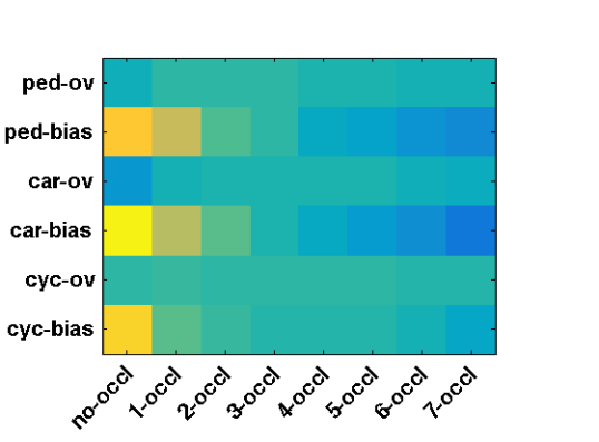
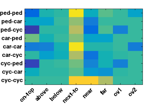
(a) inter-frame weights	(b) intra-frame weights

Figure 4: Visualization of the weight vector learned by our method. Yellow has small cost, blue has large cost. (a) shows transition weights for different length of frame jumps. The model encourages transitions to nearby neighboring frames, and penalizes long or weak transition links (i.e. overlap ratio lower than 0.5). (b) shows learned pairwise contextual weights between objects. The model encourages intra-class co-occurrence when objects are close but penalizes overlap and objects on top of others. Note the strong negative interaction learned between cyclist and pedestrian (two classes which are easily confused by their respective detectors.). By exploring contextual cues we can make correct prediction on this otherwise confusing configuration.

Dataset: We have focused our experiments on training sequences of KITTI tracking benchmark [11]. KITTI tracking benchmark consists of to 21 training sequences with a total of 8008 frames and 8 classes of labeled objects; of all the labeled objects we evaluated three categories which had sufficient number of instances for comparative evaluation: cars, pedestrians and cyclists. We use publicly available LSVM [8] reference detections and evaluation script. The evaluation script only evaluates objects that are not too far away and not truncated by more than 15 percent, it also does not consider vans as false positive for cars or sitting persons as false positive for pedestrians. The final dataset contains 636 labeled car trajectories, 201 labeled pedestrian trajectories and 37 labeled cyclists trajectories.

Training with ambiguous labels: One difficulty of training on the KITTI tracking benchmark is that it has special evaluation rules for ground truth labels such as small/truncated objects and vans for cars, sitting persons for pedestrians. This is resolved by removing all detection candidates that correspond to any of these “ambiguous” ground truth labels during training; in this way we avoid mining hard negatives from those labels. Also, to speed up training, we partition full-sized training sequences in to 10-frame-long subsequences with a 5-frame overlap, and define losses on each subsequence separately.

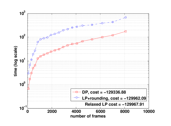
Figure 5: Speed and quality comparison of proposed undergenerating and overgenerating approximation. Over the 21 training sequences in KITTI dataset, LP+rounding produces cost that is very close to relaxed global optimum. DP gives a lower bound that is within 1% of relaxed global optimum, while being 2 to 7 times faster than a commercial LP solver (MOSEK)

Data-dependent transition model: In order to keep the size of tracking graphs tractable for our inference methods, we need a heuristic to select a sparse set of links between detection candidates across frames. We found that simply predicting candidate’s locations in future frames via optical flow gives very good performance. Specifically, we first compute frame-wise optical flow using software of [17], then for a candidate detection $x_{i}$ at frame $t_{i}$, we compute the mean of vertical flows and the mean of horizontal flows within the candidate box, and use them to predict candidate’s location in the next frame $t_{i}+1$; for $x_{i}$’s predicted locations in frame $t_{i}+2$ we use its newly predicted location at $t_{i}+1$ and candidate’s original box size to repeat the process described above, and same for $t_{i}+n$.

Trajectory smoothing: During evaluation we observe that many track fragmentation errors (FRAG) reported by the benchmark are due to the raw trajectory oscillating away from the ground-truth due to poorly localized detection candidates. Inspired by the trajectory model of  [2], we post-process each output raw trajectory by fitting a cubic B-spline. This smoothing of the trajectory eliminates many FRAGs from the raw track, making the fragmentation number more meaningful when compared across different models.

Baselines: We use the publicly available code from [10] as a first baseline. It relies on a three-stages tracklet linking scheme with occlusion sensitive appearance learning; it is by far the best tracker for cars on KITTI tracking benchmark among all published methods. Also we consider dynamic programming (DP) and successive shortest path (SSP) with default parameters in [20] as another two baselines, denoted as DP+Flow and SSP+Flow in our table.

Parameter settings: We tuned the structural parameters of the various baselines to give good performance. For all baselines we only use detections that have a positive score. For DP+Flow and SSP+Flow we also remove all transition links that have overlap ratios lower than 0.5. For learned tracking models (+Struct) we use detections that have scores greater than -0.5, and transition links that have overlap ratios greater than 0.3.

Benchmark Results: We evaluate performance using a standard battery of performance measures. The evaluation result for each object category, as well as for all categories are shown in Table 1. For our learned tracking models (+Struct) we use either network simplex solver (for SSP+Flow+Struct) or LP relaxation (for LP/DP+Flow+Struct) for training and conduct leave-one-sequence-out cross-validation with $C=2^{-9},2^{-8},...,2^{3}$. We report cross-validation result under best $C$, which is $C=2^{-8}$ for SSP+Flow+Struct and $C=2^{-7}$ for LP/DP+Flow+Struct. Our simple motion model helps DP+Flow outperform state-of-the-art baseline by a significant margin. One exception is IDSW which we attribute to the fact that the network-flow methods do not explicitly model target appearance. While SSP+Flow seems to perform poorly with default parameters, it turns out that with properly learned parameters (SSP+Flow+Struct), it produces results that are comparable to (and often better than) DP+Flow, this indicates that there is much more potential of SSP than suggested in previous work. In addition, SSP’s guarantee of optimality makes it very attractive if more complicated features and network structure are to be used in learning. As shown in Table 1, in our evaluation over all objects our model learned with pairwise costs (LP/DP+Flow+Struct) achieves the best MOTA, Recall, Mostly Tracked(MT) and Mostly Lost(ML) performance while keeping other metrics competitive.

Approximate Inference: To evaluate quality of the LP+rounding and DP approximation, we run both LP+rounding and DP inference on models trained via LP relaxation and DP respectively. We then average the running time and minimum cost found on each sequence for LP+rounding and DP, respectively. Fig 5 shows the accumulative running time and cost for each algorithm. During our experiments, LP+rounding often finds the exact relaxed global optimal, and when it doesn’t it still gives very close approximation. While greedy forward search using DP rarely reach relaxed global optimum, it still produced good approximate solutions that were often within 1% of relaxed global optimum while running significantly faster (2-7x) than LP+rounding.

Car	MOTA	MOTP	Rec	Prec	MT	ML	IDSW	FRAG
Baseline [10]	57.8	78.8	58.6	98.8	14.9	28.4	22	225
SSP+Flow	49.0	79.1	49.1	99.7	18.4	59.9	0	47
DP+Flow	62.2	79.0	63.4	98.5	25.2	24.2	43	177
SSP+Flow+Struct	63.4	78.3	65.4	97.1	27.4	20.0	2	179
LP+Flow+Struct	64.1	78.1	67.1	95.7	30.5	18.7	3	208
DP+Flow+Struct	64.6	78.0	67.5	96.0	30.1	18.6	17	222

Pedestrian	MOTA	MOTP	Rec	Prec	MT	ML	IDSW	FRAG
Baseline	40.2	73.2	49.0	86.6	4.2	32.2	132	461
SSP+Flow	37.9	73.4	41.8	92.0	8.4	57.5	25	146
DP+Flow	49.7	73.1	57.2	88.9	18.6	26.3	46	260
SSP+Flow+Struct	51.2	73.2	57.4	90.5	19.2	24.6	16	230
LP+Flow+Struct	52.6	72.9	60.2	89.2	22.2	21.6	31	281
DP+Flow+Struct	52.4	73.0	60.0	89.2	19.8	22.2	36	277

Cyclist	MOTA	MOTP	Rec	Prec	MT	ML	IDSW	FRAG
Baseline	39.0	81.6	39.6	99.5	5.4	37.8	7	26
SSP+Flow	18.7	85.6	18.7	100	5.4	89.2	0	1
DP+Flow	42.4	81.2	42.5	100	18.9	45.9	2	5
SSP+Flow+Struct	47.4	79.7	59.9	83.0	35.1	32.4	5	10
LP+Flow+Struct	52.3	79.6	61.1	88.2	40.6	27.0	12	21
DP+Flow+Struct	56.3	79.4	64.2	89.7	40.5	27.0	9	15

All Categories	MOTA	MOTP	Rec	Prec	MT	ML	IDSW	FRAG
Baseline	51.7	77.4	54.8	95.3	12.1	29.7	161	712
SSP+Flow	44.2	77.7	45.5	97.5	15.6	60.8	25	194
DP+Flow	57.6	77.4	60.5	95.7	23.5	25.7	91	442
SSP+Flow+Struct	59.0	77.0	62.8	94.5	25.9	21.5	23	419
LP+Flow+Struct	60.2	76.7	64.8	93.5	29.2	19.7	46	510
DP+Flow+Struct	60.6	76.7	65.1	93.8	28.4	19.7	62	514

Table 1: Tracking result for cars, pedestrian and cyclist categories in the KITTI tracking benchmark and aggregate performance over all categories. The proposed method using quadratic interactions between objects and parameters trained using structured prediction achieves state-of-the art MOTA and is competitive across multiple performance measures.

		Train
			DP	LP
Test	DP	MOTA	60.5	60.6
		Recall	65.2	65.1
		Precision	93.5	93.8
		MT	28.6	28.4
		ML	20.5	19.7
		IDSW	68	62
		FRAG	517	514
	LP+round	MOTA	60.1	60.2
		Recall	64.9	64.8
		Precision	93.3	93.5
		MT	29.3	29.2
		ML	20.3	19.7
		IDSW	56	46
		FRAG	518	510

Table 2: Performance evaluation over 21 sequences using cross validation for different combinations of inference algorithm used during training and test time.

Overgenerating versus Undergenerating: Previous works have shown that in general, models trained with relaxed inference are preferable than models trained with greedy inference. To investigate this idea in our particular problem, we also conduct leave-one-sequence-out cross-validation using either DP or the LP relaxation as the inference method for training. The evaluation results under different training/testing inference combinations are shown in Table 2. Notice that model trained with the LP relaxation does slightly better in most metrics, whereas DP stands out as a good inference algorithm at test time. Moreover, though slightly falling behind, model trained with greedy DP is very close to the performance of that trained with LP and thus suggests the greedy algorithm proposed here is a very competitive inference method.

7 Summary

We augmented the well-studied network-flow tracking model with pairwise cost, and proposed an end-to-end framework that jointly optimizes parameters for such model. We extensively evaluated a traditional LP relaxation-based method and a novel greedy dynamic programming method for inference in the augmented network, both of which achieves state-of-the-art performance, while our greedy DP algorithm being 2-7x faster than a commercial LP solver.

8 Acknowledgements

This work was supported by NSF DBI-1053036, IIS-1253538 and a Google Research Award.

9 Appendix: Multi-Pass Dynamic Programming to Approximate Successive Shortest Path

Now we describe two dynamic programming (DP) algorithms proposed by [20] which approximate successive shortest path (SSP) algorithm. Recall the network-flow problem described in Equation 2:

$$\underset{\mathbf{f}}{\operatorname{min}} \ \sum_{i}c_{i}^{s}f_{i}^{s}+\sum_{ij\in E}c_{ij}f_{ij}+\sum_{i}c_{i}f_{i}+\sum_{i}c_{i}^{t}f_{i}^{t}$$

s.t. $$\quad f_{i}^{s}+\sum_{j}f_{ji}=f_{i}=f_{i}^{t}+\sum_{j}f_{ij}$$

$$f_{i}^{s},f_{i}^{t},f_{i},f_{ij}\in\{0,1\}$$

The corresponding graphical model is shown in Fig 6. SSP finds the global optimum of Objective 2 by repeating: 1. Find the minimum cost source to sink path on residual graph $G_{r}(\mathbf{f})$
2. If the cost of the path is negative, push a flow through the path to update $\mathbf{f}$ Until no negative cost path can be found. A residual graph $G_{r}(\mathbf{f})$ is the same as the original graph $G$ except all edges in $\mathbf{f}$ are reversed and their cost negated. We focus on describing the DP algorithms and refer readers to [1] for detailed description of SSP algorithm.

9.1 One-pass DP

Assume the detection nodes are sorted in time. We denote $cost(i)$ as the cost of the shortest path from source node to node $i$, $link(i)$ as $i$’s predecessor in this shortest path, and $birth\_node(i)$ as the first detection node in this shortest path. We initialize $cost(i)=c_{i}+c_{i}^{s}$, $link(i)=\emptyset$, and $birth\_node(i)=i$ for all $i\in V$.

To find the shortest path on the initial DAG $G$, we can sweep from first frame to last frame, computing $cost(i)$ as:

$$cost(i)=c_{i}+\text{min}(\pi,c_{i}^{s}),\;\pi=\underset{ji\in E}{\operatorname{min}}\;c_{ji}+cost(j)$$ (11)

And update $birth\_node(i)$, $link(i)$ accordingly.

After we sweeping through all frames, we find a node $i$ such that $cost(i)+c_{i}^{t}$ is minimum, and reconstruct the shortest path by backtracking cached $link$ variables. The cost of this path would be $cost(i)+c_{i}^{t}$. After the shortest path is found, we remove all nodes and edges in this shortest path from $G$, the resulting graph $G^{\prime}$ will still be a DAG, thus we can repeat this procedure until we cannot find any path that has a negative cost. Even more speed up can be achieved by only recomputing $cost(i)$, $birth\_node(i)$ and $link(i)$ for those $i$ whose birth node is the same as the birth node of the track found in previous iteration.

It is also straightforward to integrate NMS into this algorithm: when we pick up a shortest path, we also prune all nodes that overlap the shortest path. In practice this ”temporal NMS” can be much more aggressive than pre-processing NMS, since the confidence of a track being composed of true positives is much higher than single detections.

9.2 Two-pass DP

Figure 6: Graphical representation of network flow model from [27]. A pair of nodes (connected by red edge) represent a detection, blue edges represent possible transitions between detections and birth/death flows are modeled by black edges. Costs $c_{i}$ in Objective 2 are for red edges, $c_{ij}$ are for blue edges, $c_{i}^{t}$ and $c_{i}^{s}$ are for black edges. To simplify our description, we will refer a detection edge and the two nodes associated with it as a ”node” or ”detection node”. The set $V$ consists of all detection nodes in the graph, whereas the set $E$ consists of all transition edges in the graph.

2-pass DP works very similarly to successive shortest path, the only difference is that instead of using Dijkstra’s algorithm, we use two passes of dynamic programming to approximate shortest path on the residual graph $G_{r}(\mathbf{f})$. We denote $V_{forward}$ as the set of forward nodes in current residual graph, and $V_{backward}$ as the set of backward nodes in current residual graph, we describe one iteration of 2-pass DP as below: 1. Ignore all backward edges (including reversed detection edges) and perform one pass of forward DP (from first frame to last frame) on all nodes. For each node $i$, there will be a $path(i)$ array that stores mininum-cost source to $i$ path, with $cost(i)$ being the total cost of this path.
2. Use $cost(i)$ from step 1 as initial values and perform one pass of backward DP (from last frame to first frame) on $V_{backward}$. After this, $cost(i)$ for $i\in V_{backward}$ would be the $cost(j)-c_{ij}$, where $j$ is $i$’s best (backward) predecessor and $c_{ij}$ is from the original graph. Set $cost(i)=+\infty$ for backward node $i$ that has no backward edge coming to it.
3. Perform one pass of forward DP on $i\in V_{forward}$. To avoid running into cyclic path, we need to backtrack shortest paths for all $j\in N(i)$, where $N(i)$ is all neighboring nodes that are connected to $i$ via a forward edge.
4. Find node $i$ with minimum $cost(i)+c_{i}^{t}$, the (approximate) shortest path is then $path(i)$.
5. Update solution $\mathbf{f}$ by setting all forward variables along $path(i)$ to 1 and all backward variables along $path(i)$ to 0. It is straightforward to show that during the first iteration, 1-pass DP and 2-pass DP behave identically. Also, the path found by 2-pass DP will never go into a source node or go out of a sink node, thus in each iteration we generate exactly one more track, either by splitting a previously found track, or by choosing a entirely new track. Therefore the algorithm will terminate after at most $|V|$ iterations.

10 Appendix: Incorporating Quadratic Interactions in Multi-pass DP

Recall the augmented network-flow problem with quadratic cost (Eqn. 4):

$$\begin{split}\underset{\mathbf{f}}{\operatorname{min}}&\sum_{i}c_{i}^{s}f_{i}^{s}+\sum_{ij\in E}c_{ij}f_{ij}+\sum_{i}c_{i}f_{i}\\ &+\sum_{ij\in EC}q_{ij}f_{i}f_{j}+\sum_{i}c_{i}^{t}f_{i}^{t}\end{split}$$

s.t. $$\quad f_{i}^{s}+\sum_{j}f_{ji}=f_{i}=f_{i}^{t}+\sum_{j}f_{ij}$$

$$f_{i}^{s},f_{i}^{t},f_{i},f_{ij}\in\{0,1\}$$

Where $EC=\{ij:t_{i}=t_{j}\}$. We propose two new variants of DP algorithm that can approximately minimize the Objective 4. They are also divided into 1-pass DP and 2-pass DP. Since we already described 1-pass DP with pairwise interactions in the paper, we will focus on 2-pass DP with pairwise interactions here.

10.1 Two-pass DP with quadratic interactions

A feasible solution $\mathbf{f}$ on the network corresponds to a residual graph $G_{r}(\mathbf{f})$. We could apply the steps described in section 9.2 to find an approximate shortest path. This path may consist of both forward nodes and backward nodes, which correspond to uninstanced detections (but will be instanced after this iteration) and already instanced detections (but will be uninstanced after this iteration) respectively. We then update the (unary) cost of other nodes by adding or subtracting the pairwise cost imposed by turning on or off selected nodes on the path. Additionally, at step 3 of 2-pass DP, one could also consider the pairwise cost to current node imposed by previously selected nodes in the same path. The entire procedure is described as Algorithm 2.

Algorithm 2 Two-pass DP with pairwise Cost Update

1:Input: A Directed-Acyclic-Graph $G$ with node and edge weights $c_{i},c_{ij}$

2:initialize $\mathbf{f}=\mathbf{0}$

3:repeat

4:     Find start-to-end min-cost unit flow $\mathbf{f}^{*}$ on $G_{r}(\mathbf{f})$

5:     $track\_cost=cost(\mathbf{f}^{*})$

6:     if $track\_cost<0$ then

7:         for all $f_{i}\in\mathbf{f}^{*}$ do

8:              if $f_{i}=0$ then

9:                  $c_{j}=c_{j}+q_{ij}+q_{ji},\forall ij,ji\in EC$

10:              else

11:                  $c_{j}=c_{j}-q_{ij}-q_{ji},\forall ij,ji\in EC$

12:              end if

13:         end for

14:         $\mathbf{f}^{*}=\neg\mathbf{f}^{*}$

15:     end if

16:until $track\_cost\geq 0$

17:Output: Solution $\mathbf{f}$

Notice that, to simplify our notation, we construct temporary residual graph at the beginning of each iteration and do not negate edge weights in the original graph. In practice, we can instead update edge costs and directions on the original graph at the end of each iteration, in such a case we should add pairwise costs to forward nodes or subtract pairwise costs from backward nodes if we turn on some node, similarly we subtract pairwise costs from forward nodes or add pairwise costs to backward nodes if we turn off some node.

10.2 Approximation Quality of Two-pass DP

We found that 2-pass DP often finds lower cost than 1-pass DP but still not as good as LP+rounding. It also runs significantly slower, even slower than LP+rounding on long sequences. On a 1059 frame-long video with 3 categories of objects, 2-pass DP uses about 6 minutes to finish, whereas 1-pass DP finishes within 1 minute and LP+rounding finishes within 4 minutes. The leave-one-sequence-out cross-validation result using 2-pass DP gets a MOTA of 60.4%, which is equivalent to that of 1-pass DP and LP relaxation.

We observe that most of the running time for 2-pass DP is on the second forward pass, which involves backtracking for each forward node to avoid cyclic path. It should be noted that with proper data structure such as a hash linked-list to cache $path$ arrays, checking cyclic path can be done in $O(1)$. Also, in the second forward pass, one could set all backward nodes as active and propagate active labels to other forward nodes, so eventually we might not need to look at every forward node. Overall, though showing some incompetence in running time in our current implementation, 2-pass DP should still be a promising inference method with better choice of data-structures and moderate optimization.

(a)

(b)

(c)

(d)

(e)

Figure 7: An illustration for 2-pass DP with quadratic interactions. (a) the initial DAG graph, a pair of nodes indicate a candidate detection; (b) first iteration of the algorithm, red edges indicates the shortest path found in this iteration; (c) we reverse all the edges on the shortest path (green edges), and add the pairwise cost imposed by this path to other candidates within the time window (red pairs); (d) second iteration of algorithm, red edges and blue edges indicates the new shortest path, notice that it takes three of reversed edges (blue edges); (e) we again reverse all the edges in the shortest path, now green edges indicate the two tracks found in this 2 iterations; we also update pairwise cost: blue node pair indices we subtract the pairwise cost imposed by ”turning off” an candidate, red pair still indicates adding in pairwise cost of newly instanced candidates,and the blue-red pair indicates we first add the pairwise cost by newly instanced candidates, then subtract the pairwise cost by newly uninstanced candidates. Additions and subtractions are done to the non-negated edge costs and then negated if necessary.

References

- [1] R. K. Ahuja, T. L. Magnanti, and J. B. Orlin. Network Flows: Theory, Algorithms, and Applications. Prentice-Hall, Inc., Upper Saddle River, NJ, USA, 1993.
- [2] A. Andriyenko, K. Schindler, and S. Roth. Discrete-continuous optimization for multi-target tracking. In CVPR, 2012.
- [3] K. Bernardin and R. Stiefelhagen. Evaluating multiple object tracking performance: The clear mot metrics. J. Image Video Process., 2008:1:1–1:10, Jan. 2008.
- [4] W. Brendel, M. Amer, and S. Todorovic. Multiobject tracking as maximum weight independent set. In In Proc. IEEE Conf. on Computer Vision and Pattern Recognition, 2011.
- [5] A. A. Butt and R. T. Collins. Multi-target tracking by lagrangian relaxation to min-cost network flow. In The IEEE Conference on Computer Vision and Pattern Recognition (CVPR), June 2013.
- [6] V. Chari, S. Lacoste-Julien, I. Laptev, and J. Sivic. On pairwise cost for multi-object network flow tracking. CoRR, abs/1408.3304, 2014.
- [7] C. Desai, D. Ramanan, and C. Fowlkes. Discriminative models for multi-class object layout. In IEEE International Conference on Computer Vision, 2009.
- [8] P. F. Felzenszwalb, R. B. Girshick, and D. McAllester. Discriminatively trained deformable part models, release 4. http://people.cs.uchicago.edu/ pff/latent-release4/.
- [9] T. Finley and T. Joachims. Training structural SVMs when exact inference is intractable. In International Conference on Machine Learning (ICML), pages 304–311, 2008.
- [10] A. Geiger, M. Lauer, C. Wojek, C. Stiller, and R. Urtasun. 3d traffic scene understanding from movable platforms. Pattern Analysis and Machine Intelligence (PAMI), 2014.
- [11] A. Geiger, P. Lenz, and R. Urtasun. Are we ready for autonomous driving? the kitti vision benchmark suite. In Conference on Computer Vision and Pattern Recognition (CVPR), 2012.
- [12] T. Joachims, T. Finley, and C.-N. Yu. Cutting-plane training of structural svms. Machine Learning, 77(1):27–59, 2009.
- [13] A. Joulin, K. Tang, and L. Fei-Fei. Efficient image and video co-localization with frank-wolfe algorithm. In European Conference on Computer Vision (ECCV), 2014.
- [14] S. Kim, S. Kwak, J. Feyereisl, and B. Han. Online multi-target tracking by large margin structured learning. In Proceedings of the 11th Asian Conference on Computer Vision - Volume Part III, ACCV’12, pages 98–111, Berlin, Heidelberg, 2013. Springer-Verlag.
- [15] S. Lacoste-Julien, B. Taskar, D. Klein, and M. I. Jordan. Word alignment via quadratic assignment. In Proceedings of the Main Conference on Human Language Technology Conference of the North American Chapter of the Association of Computational Linguistics, HLT-NAACL ’06, pages 112–119, Stroudsburg, PA, USA, 2006. Association for Computational Linguistics.
- [16] Y. Li, C. Huang, and R. Nevatia. Learning to associate: Hybridboosted multi-target tracker for crowded scene. In In CVPR, 2009.
- [17] C. Liu. Beyond Pixels: Exploring New Representations and Applications for Motion Analysis. PhD thesis, Massachusetts Institute of Technology, 2009.
- [18] X. Lou and F. A. Hamprecht. Structured Learning for Cell Tracking. In Twenty-Fifth Annual Conference on Neural Information Processing Systems (NIPS 2011), 2011.
- [19] A. Milan, K. Schindler, and S. Roth. Detection- and trajectory-level exclusion in multiple object tracking. In CVPR, 2013.
- [20] H. Pirsiavash, D. Ramanan, and C. C. Fowlkes. Globally-optimal greedy algorithms for tracking a variable number of objects. In IEEE conference on Computer Vision and Pattern Recognition (CVPR), 2011.
- [21] M. Szummer, P. Kohli, and D. Hoiem. Learning crfs using graph cuts. In European Conference on Computer Vision, October 2008.
- [22] B. Taskar, C. Guestrin, and D. Koller. Max-margin markov networks. MIT Press, 2003.
- [23] B. Wang, G. Wang, K. Luk Chan, and L. Wang. Tracklet association with online target-specific metric learning. In The IEEE Conference on Computer Vision and Pattern Recognition (CVPR), June 2014.
- [24] Z. Wu, A. Thangali, S. Sclaroff, , and M. Betke. Coupling detection and data association for multiple object tracking. In Proceeding of the IEEE Conference on Computer Vision and Pattern Recognition (CVPR), pages 1–8, Rhode Island, June 2012.
- [25] B. Yang and R. Nevatia. An online learned crf model for multi-target tracking. In In CVPR, 2012.
- [26] A. N. H. Zaied and L. A. E. fatah Shawky. Article: A survey of quadratic assignment problems. International Journal of Computer Applications, 101(6):28–36, September 2014. Full text available.
- [27] L. Zhang, Y. Li, and R. Nevatia. Global data association for multi-object tracking using network flows. 2013 IEEE Conference on Computer Vision and Pattern Recognition, 0:1–8, 2008.