Robust Output Regulation of
Linear Passive Systems with
Multivalued Upper Semicontinuous Controls

Abstract

The use of multivalued controls derived from a special maximal monotone operator are studied in this note. Starting with a strictly passive linear system (with possible parametric uncertainty and external disturbances) a multivalued control law is derived, ensuring regulation of the output to a desired value. The methodology used falls in a passivity-based control context, where we study how the multivalued control affects the dissipation equation of the closed-loop system, from which we derive its robustness properties. Finally, some numerical examples together with implementation issues are presented to support the main result.

1 Introduction

Sometimes it is useful to have an interpretation of the action of the controller in energetic terms. Among the most important methodologies of passivity-based control (PBC) that achieve this interpretation are the so-called energy shaping techniques. The purpose of energy shaping, as its name suggests, is to change the energy function (by means of the control action) in such a way that stabilization and performance objectives are satisfied. Although energy-shaping strategies have proved to be very useful yielding an easy interpretation of the controller in energetic terms [16], robustness against external perturbations and model uncertainty is still a topic of research.

On the other hand, the study of differential inclusions for modelling and analysis of processes in control theory is extensive (e.g. [1, 8, 13]), whereas the problem of designing a multivalued control in order to achieve a desired response is less explored, except for the case of sliding mode control, which takes advantage of the multivalued nature of the signum multifunction in order to ensure robustness of the closed-loop system.

An important family of differential inclusions (more general than those obtained by using sliding modes techniques) are those for which its right-hand side is represented by maximal monotone operators. In the case of linear plants, the closed-loop system is sometimes called a multivalued Lur’e dynamical system, for which results about existence and uniqueness of solutions have been proved in [2, 4, 5, 22]. This kind of systems are related to complementarity and projected dynamical systems [3], which makes its study important for a broad range of applications coming from different fields such as automatic control, economics, mechanics, etc.

The main contribution of this note consists in a design procedure for a multivalued-control — where the multivalued part is represented by the subdifferential of some proper, convex and lower semicontinuous function — which achieves finite-time regulation of the desired output together with insensitivity against a family of bounded and unmatched perturbations.

The proposed multivalued control strategy differs remarkably from those which are common in Sliding-Mode Control in the sense that we obtain finite-time regulation and disturbance rejection without a discontinuous right-hand side and therefore without the necessity of solutions of the associated system in the the sense of Filippov.

This note is organized as follows. In Section 2 the class of systems that we consider is established in conjunction with the class of perturbations that it will be treated. The multivalued structure of the controller is presented and well-posedness of the closed-loop system is established. In Section 3, we introduce the main result of this note. Namely, robustness and finite time convergence of the closed-loop system are demonstrated. Section 4 touches the point about implementation of the multivalued control law by introducing a regularization of the multivalued map. Some examples are presented showing the closed loop properties. The note ends with some conclusions and future research lines in Section 5.

1.1 Notations and some basics

Throughout this note, all vectors are column vectors, even the gradient of a scalar function that we denote by $\nabla H(x)=\frac{\partial H(x)}{\partial x}$. A matrix $A\in\mathbb{R}^{n\times n}$ is called positive definite (denoted as $A>0$), if $w^{\top}Aw>0$ for all $w\in\mathbb{R}^{n}\setminus\{0\}$ (note that we are not assuming $A$ symmetric).

A set-valued function or multifunction $\mathbf{F}:\mathbb{R}^{n}\to 2^{\mathbb{R}^{n}}$ is a map that associates with any $w\in\mathbb{R}^{n}$ a subset $\mathbf{F}(w)\subset\mathbb{R}^{n}$. The domain of $\mathbf{F}$ is given by

$$\operatorname{Dom}\mathbf{F}=\{w\in\mathbb{R}^{n}:\mathbf{F}(w)\neq\emptyset\}\;,$$

related with the definition of a multifunction is the concept of its graph,

$$\operatorname{Graph}\mathbf{F}=\{(w,z)\in\mathbb{R}^{n}\times\mathbb{R}^{n}:z\in\mathbf{F}(w)\}\;.$$

The graph is used to define the concept of monotonicity of a multifunction in the following way: A set-valued function $\mathbf{F}$ is said to be monotone if for all $(w,z)\in\operatorname{Graph}\mathbf{F}$ and all $(w^{\prime},z^{\prime})\in\operatorname{Graph}\mathbf{F}$ the relation

$$\langle z-z^{\prime},w-w^{\prime}\rangle\geq 0$$

is preserved, where $\langle\cdot,\cdot\rangle$ denotes the usual scalar product on $\mathbb{R}^{n}$. A monotone map $\mathbf{F}$ is called maximal monotone if, for every pair $(\hat{w},\hat{z})\in\mathbb{R}^{n}\times\mathbb{R}^{n}\setminus\operatorname{Graph}\mathbf{F}$, there exits $(w,z)\in\operatorname{Graph}\mathbf{F}$ with $\langle z-\hat{z},w-\hat{w}\rangle<0$, or in other words, if no enlargement of its graph is possible in $\mathbb{R}^{n}\times\mathbb{R}^{n}$ without destroying monotonicity.

Let $f:\mathbb{R}^{n}\to\mathbb{R}\cup\{+\infty\}$ be a proper, convex and lower semi-continuous function. The effective domain of $f$ is given by

$$\operatorname{Dom}f=\{w\in\mathbb{R}^{n}:f(w)<\infty\}\;.$$

We say that $f$ is proper if its effective domain is non empty. The subdifferential $\partial f(w)$ of $f(\cdot)$ at $w\in\mathbb{R}^{n}$ is defined by

$$\partial f(w)=\{\zeta\in\mathbb{R}^{n}:f(\sigma)-f(w)\geq\langle\zeta,\sigma-w\rangle\text{ for all }\sigma\in\mathbb{R}^{n}\}\;.$$

An important convex function is the indicator function of a convex set $S$, defined by

$$\psi_{\mathcal{S}}(w)=\begin{cases}0&\mbox{if }w\in S\\ +\infty&\mbox{if }w\notin S\end{cases}\;.$$

It is easy to see that when $f(\cdot)$ is equal to the indicator function of a closed convex set $S$, then the subdifferential coincides with the normal cone of the set $S$ at the point $w\in S$, i.e.,

$$\partial\psi_{S}(w)=N_{S}(w)=\{\xi\in\mathbb{R}^{n}:0\geq\langle\xi,\sigma-w\rangle\text{ for all }\sigma\in S\}\;.$$

Note that if $w$ is in the interior of $S$ then $N_{S}(w)=\{0\}$. If $w\notin S$ then $N_{S}(w)=\emptyset$.

2 The output regulation problem

Consider the following affine system:

$$\Sigma:\begin{cases}\dot{x}(t)=Ax(t)+B_{\mathrm{u}}u_{1}(t)+B_{\mathrm{v}}v(t)\cr y_{1}(t)=Cx(t)+Du_{1}(t)\end{cases}\;,$$ (2.1)

where $x\in\mathbb{R}^{n}$ denotes the system state, $u_{1},y_{1}\in\mathbb{R}^{m}$ are the port variables available for interconnection, which are conjugated in the sense that their product has units of power, and matrices $A,B_{\mathrm{u}},B_{\mathrm{v}},C,D$ are constant and of suitable dimensions. The term $v\in\mathbb{R}^{m}$ accounts for an uncertain exogenous input which is considered bounded. Moreover, without loss of generality, the external signal $v(t)$ can be decomposed as the sum of a constant term $v^{+}$ and a bounded signal $\nu(t)$.

The robust output regulation problem consists in regulating the output $y_{1}$ to a desired value $y_{\mathrm{d}}$, even in the presence of the external perturbation $v(t)$ and parametric uncertainties.

Remark 1.

Notice that, for $D=0$ and $B_{\mathrm{u}}=B_{\mathrm{v}}$ , the problem reduces to a standard sliding-mode control problem with matched disturbances. We depart from these standard assumptions and make the following instead.

Assumption 1.

There exists a (possibly unknown) matrix $P=P^{\top}>0$ such that

$$\begin{bmatrix}PA+A^{\top}P&PB_{\mathrm{u}}-C^{\top}\\ B_{\mathrm{u}}^{\top}P-C&-(D+D^{\top})\end{bmatrix}<0\;.$$ (2.2)

Assumption 1 is a rewrite of the strict passivity property of plant (2.1) with respect to the input $u_{1}$ and output $y_{1}$ [12]. Moreover, is easy to see that the passivity assumption implies that $D$ is positive definite. Equivalently, Assumption 1 can be rewritten in terms of the energy-balance equation. More precisely, there exists a continuously differentiable function $H:\mathbb{R}^{n}\to\mathbb{R}$, called the storage function, such that for all $t\geq 0$ we have

$$H(x(t))-H(x(0))=\int_{0}^{t}u_{1}^{\top}(\tau)y_{1}(\tau)d\tau-\mathrm{d}(t)\;,$$

where the function $\mathrm{d}(t)\geq 0$ is associated to the dissipation of the system and the storage function $H(x)$ is bounded from below (see, e.g., [16]).

Remark 2.

The strict passivity assumption allows us to admit the quadratic function $H_{0}(x)=x^{\top}Px$ as a storage function with $P$ satisfying (2.2).

It is worth noting that in the linear case, the class of passive systems is equivalent to the class of Port-Hamiltonian (PH) systems described in [20, Ch. 4], i.e., $\Sigma$ can be written as

$$\dot{x} =F\nabla H_{0}(x)+g_{\mathrm{u}}u_{1}+g_{\mathrm{v}}v$$

$$y_{1} =h(x)+ju_{1}$$

with $F=AP^{-1}=J-R$, where $J=-J^{\top}$ and $R=R^{\top}\geq 0$ are the so called interconnection and dissipation matrices, respectively, $g_{\mathrm{u}}=B_{\mathrm{u}}$, $g_{\mathrm{v}}=B_{\mathrm{v}}$, $h(x)=Cx$ and $j=D$.

Along this note we will use both representations of $\Sigma$ with the purpose of expressing the related computations in the context of basic interconnection and damping assignment (IDA) [17, 20].

2.1 Multivalued control law

In this subsection a multivalued control law is introduced by using maximal monotone operators. It will be shown later on that these are robust in the face of parametric and additive uncertainties.

Let $u_{2}\in\mathbb{R}^{m}$ and $y_{2}\in\mathbb{R}^{m}$ be the port variables available for interconnection associated to the controller. The multivalued control input is defined in terms of the graph of a multifunction $\mathbf{U}:\mathbb{R}^{m}\to 2^{\mathbb{R}^{m}}$ by

$$(u_{2},y_{2})\in\operatorname{Graph}\mathbf{U}\;.$$

Remark 3.

It is worthy to mention that, in the case when the multifunction $\mathbf{U}$ is monotone, the relation $(u_{2},y_{2})\in\operatorname{Graph}\mathbf{U}$ defines a static, incrementally passive map. Furthermore, if $0\in\mathbf{U}(0)$, then the relation between $u_{2}$ and $y_{2}$ defines a static passive map inasmuch as

$$\langle u_{2},y_{2}\rangle\geq 0\text{ for all }(u_{2},y_{2})\in\operatorname{Graph}\mathbf{U}\;.$$

Previous lines motivate the following assumption.

Assumption 2.

The multifunction $\mathbf{U}$ is maximal monotone, and defines a static passive relation between the input $u_{2}$ and the output $y_{2}$.

The multivalued nature of the proposed control motivates us to depart from the classical intelligent control paradigm and to make use of the behavioural framework proposed by Willems [21] instead. In this context, the plant and the controller are interconnected using a power preserving pattern as shown in Figure 1 satisfying: $y_{1}=y_{2}=:y$, $-u_{1}=u_{2}=:u$ and therefore

$$u_{1}y_{1}+u_{2}y_{2}=0\;.$$

Figure 1: Interconnection of a controller to a plant.

The interconnected system (plant and controller) results in

$$\dot{x} =Ax-B_{\mathrm{u}}u+B_{\mathrm{v}}v$$ (2.3a)

$$y =Cx-Du$$ (2.3b)

$$u \in\mathbf{U}(y)\;,$$ (2.3c)

where our task is to determine $\mathbf{U}(y)$ such that $y$ is regulated to some fixed value $y_{\mathrm{d}}$, even in the presence of uncertainties in the system parameters and the external perturbation $v$. Note that the previous argument rules out the trivial control $u=D^{-1}(Cx-y_{\mathrm{d}})$. In fact, even if all the system parameters and the state $x$ were known, that control would not be admissible, since it is not passive (see Assumption 2).

It is well known that when $\mathbf{U}(y)$ is given as the subdifferential of a proper, convex and lower semicontinuous function $\Phi(\cdot)$ (i.e. $\mathbf{U}(y)=\partial\Phi(y)$), it is a maximal monotone operator [18, Cor. 31.5.2]. Therefore, we will focus on controls of the form

$$u\in\partial\Phi(y)\;,$$ (2.4)

for some proper, convex and lower semicontinuous function $\Phi:\mathbb{R}^{m}\to\mathbb{R}^{m}$. More specifically, in Section 3 we will prove that, for some closed convex set $S$, robust regulation of the output $y$ is obtained for the case when $\Phi(y)=(\varphi+\psi_{S})(y)$, where $\varphi(\cdot)$ is proper, convex and lower semicontinuous with effective domain containing $S$ and $\psi_{S}(\cdot)$ is the indicator function of the set $S$. In other words, $\Phi$ is the restriction of $\varphi$ to $S$.

2.2 Well-posedness

Before presenting the main result of this note about robustness of the closed-loop system (2.3), is important first to establish its well-posedness. Specifically, well-posedness of the closed-loop system comprises two issues. The first question is: Is there always a control input $u\in\partial\Phi(y)$? and the second one is about uniqueness and existence of solutions of the associated differential inclusion (2.3).

For the second issue about a solution of the differential inclusion (2.3), well-posedness was proved previously in [4, 5], where the subdifferential of the conjugate function of $\Phi(y)$ together with passivity of the associated system plays a crucial role.

The first issue deserves more explanation. At first we need $y\in S$ for all time $t$, this comes from the definition of the subdifferential, i.e., $u\in\partial\Phi(y)$ is equivalent to

$$\Phi(\sigma)-\Phi(y)\geq\langle u,\sigma-y\rangle\text{ for all }\sigma\in\mathbb{R}^{m}\;,$$

where, in the case of $\Phi(y)=(\varphi+\psi_{S})(y)$ we have

$$\varphi(\sigma)-\varphi(y)+\psi_{S}(\sigma)-\psi_{S}(y)\geq\langle u,\sigma-y\rangle\text{ for all }\sigma\in\mathbb{R}^{m}\;,$$ (2.5)

and it is clear that if $y\notin S$, then we will have $\partial\Phi(y)=\emptyset$. Then, we must guarantee that, no matter what the initial conditions are, it is possible to find an output $y\in S$, such that $u\in\partial\Phi(y)$ is well defined.

In the case where $\varphi\equiv 0$ and the matrix $D$ is symmetric, well-posedness is easy to show. Since $u\in\partial\psi_{S}(y)=N_{S}(y)$, from the definition of normal cone we have

$$0\geq\langle u,\sigma-y\rangle\text{ for all }\sigma\in S\;,$$

which in view of (2.3b) translates to

$$0\geq\langle D^{-1}(Cx-y),\sigma-y\rangle=(\sigma-y)^{\top}D^{-1}(Cx-y)=\langle Cx-y,\sigma-y\rangle_{D^{-1}}$$

¡++¿ for all $\sigma\in S$, with the inner product weighted by $D^{-1}$. From [10, p. 117] we have that the above inequality is the characterization of the projection of $Cx$ onto the set $S$ with the induced norm $\|\cdot\|_{D^{-1}}$, i.e.

$$y=\operatorname{Proj}_{S}^{D^{-1}}(Cx)=\operatorname*{arg\,min}_{\sigma\in S}\|Cx-\sigma\|_{D^{-1}}\;,$$ (2.6)

and the control input $u$ transforms into

$$u=D^{-1}\left(Cx-\operatorname{Proj}_{S}^{D^{-1}}(Cx)\right)\in N_{S}(y)\;.$$ (2.7)

Therefore, in the case of $D$ symmetric, we can find an expression for the output $y$ in terms of the projection operator $\operatorname{Proj}_{S}^{D^{-1}}(\cdot)$ (note that this implies $y\in S$ independently of the state $x$). Moreover, due to the Lipschitzian property of the projection operator [10, p. 118], substitution of $u$ in (2.3) leads to a well-posed ordinary differential equation (not a differential inclusion!) with a Lipchitzian right-hand side (see [14] for a detailed development in the scalar case).

For the general case where $\varphi$ is not the zero function, and removing the assumption about the symmetry of $D$, from (2.5) we have that the problem consists in finding $y\in S$ such that

$$0\leq\langle D^{-1}y-D^{-1}Cx,\sigma-y\rangle+\varphi(\sigma)-\varphi(y)\text{ for all }\sigma\in S\;,$$ (2.8)

where we made use of (2.3b). The inequality (2.8) is an hemivariational inequality, for which existence and uniqueness of solutions can be deduced from $D^{-1}$ as the following Lemma extracted from [9] shows.

Lemma 1 (Lemma 5.2.1, [9]).

Suppose that $F(y)$ is continuous and strongly monotone, i.e.

$$\langle F(y)-F(y^{\prime}),y-y^{\prime}\rangle\geq\eta\|y-y^{\prime}\|^{2}$$

for all $y,y^{\prime}\in\mathbb{R}^{m}$ and some $\eta>0$. Then, for each $g\in\mathbb{R}^{n}$ there exists an unique solution $y^{*}\in S$ to

$$\langle F(y)-g,\sigma-y\rangle+\Phi(\sigma)-\Phi(y)\geq 0\text{ for all }\sigma\in S\;.$$

Since $D$ is positive definite, it is straightforward to see that $D^{-1}$ is positive definite too. Furthermore, the linear map $y\mapsto D^{-1}y$ is strongly monotone (as a consequence of applying Rayleigh’s inequality). Then using Lemma 1 we have that the hemivariational inequality problem (2.8) has a unique solution for each state $x$. In other words: For all $x\in\mathbb{R}^{n}$, there always exists a unique $y\in S$ such that the control $u\in\partial\Phi(y)$ is well defined.

Remark 4.

The computation of the control input which forces $y\in S$ obviously depends on the solution of the hemivariational inequality (2.8) and therefore it depends implicitly on the actual state of the plant $x$. This dependency of the state, induces a partition in the phase space.

Remark 5.

For the case when $\varphi\equiv 0$ and $D$ is symmetric, we might be tempted to use (2.7) as control input (because it is passive), but unfortunately it is not implementable in our setting because it depends explicitly on the system parameters and state. The role of (2.7) is analogous to the role of the equivalent control in sliding modes [19], in the sense that it is not implementable but helps to determine the dynamics associated to the closed-loop system. See [14] for an example of the use of the control (2.7) in the scalar case and some implementation issues.

Following the steps in [14], the control that results from the solution of the hemivariational inequality (2.8) will act as an equivalent control, in the sense of Remark 5 and is not implementable under the assumption that the state and the plant parameters are unknown. The implemented control is described in Section 4.

3 Finite-time perfect output regulation

The main result of this note is presented in this section. Namely, from an energy-shaping point of view, we show that the multivalued control (2.4) can be expressed as a basic IDA controller plus a robustifying term denoted by $\eta$, affecting directly the dissipation of the closed-loop system and yielding to the output regulation despite the presence of external and parametric disturbances.

From the closed-loop equation of the system, we have

$$\dot{x} =Ax-B_{\mathrm{u}}u+B_{\mathrm{v}}v$$ (3.1a)

$$y =Cx-Du$$ (3.1b)

$$u \in\partial\Phi(y)$$ (3.1c)

with $\Phi(\cdot)=(\varphi+\psi_{S})(\cdot)$ for some convex set $S$. The perturbation input $v(t)$, decomposed as a constant term $v^{+}$ and a bounded unknown signal $\nu(t)$, affects the dissipation equation in the following way.

Let $\bar{x}$ be the equilibrium point of (3.1) associated to a constant perturbation ($\nu(t)\equiv 0$) and input $u=0$, i.e.,

$$0=A\bar{x}+B_{\mathrm{v}}v^{+}\;,$$ (3.2)

and let $H_{0}$ be the storage function of system (3.1) (i.e. $H_{0}(x)=x^{\top}Px$ with $P$ satisfying (2.2)). We obtain

$$0 =F\nabla H_{0}(\bar{x})+B_{\mathrm{v}}v^{+}$$

$$=F\nabla H_{0}(\bar{x})\pm F\nabla H_{0}(x)+B_{\mathrm{v}}v^{+}$$

$$=-F\left(\nabla H_{1}(x)-\nabla H_{0}(x)\right)+B_{\mathrm{v}}v^{+}$$

with $H_{1}(x)=(x-\bar{x})^{\top}P(x-\bar{x})$. Now, defining $H_{a}(x)=H_{1}(x)-H_{0}(x)$ we have the basic IDA controller equation [6] for $v^{+}$ as

$$F\nabla H_{a}(x)=B_{\mathrm{v}}v^{+}\;.$$

Then, we have that the term $v^{+}$ acts as an energy-shaping control changing the storage function of the uncontrolled system $H_{0}$ to $H_{1}$ and therefore changing the equilibrium of the system. The closed-loop system results in

$$\dot{x} =F\nabla H_{1}(x)-B_{\mathrm{u}}u+B_{\mathrm{v}}\nu$$ (3.3a)

$$y =Cx-Du$$ (3.3b)

$$u \in\partial\Phi(y)$$ (3.3c)

For the case $\nu=0$, a control input can be designed in order to obtain the asymptotic regulation of the output $y$ to $y_{\mathrm{d}}$ using an energy-shaping interpretation as follows.

Lemma 2.

For system (3.3), let $x_{*}$ be an admissible equilibrium associated to the constant control $\bar{u}=D^{-1}(Cx_{*}-y_{\mathrm{d}})$, i.e. $x_{*}$ satisfies

$$0=Ax_{*}-B_{\mathrm{u}}D^{-1}(Cx_{*}-y_{\mathrm{d}})+B_{\mathrm{v}}v^{+}\;.$$ (3.4)

Then, $\bar{u}$ achieves regulation of the output to $y_{\mathrm{d}}$ when $\nu=0$. Furthermore, $\bar{u}$ is a basic IDA controller and satisfies

$$F\nabla H_{b}(x)=-B_{\mathrm{u}}\bar{u}\;,$$

with $H_{b}(x)=H_{2}(x)-H_{1}(x)$ and $H_{2}(x)=(x-x_{*})^{\top}P(x-x_{*})$.

Proof.

Let $x_{*}$ be an equilibrium of system (3.3) satisfying (3.4). Then, from (3.2) we have that

$$0=A(x_{*}-\bar{x})-B_{\mathrm{u}}D^{-1}(Cx_{*}-y_{\mathrm{d}})\;,$$

or, in terms of the storage functions $H_{1}$ and $H_{2}$,

$$0=-F(\nabla H_{2}(x)-\nabla H_{1}(x))-B_{\mathrm{u}}D^{-1}(Cx_{*}-y_{\mathrm{d}})\;.$$

Therefore, we obtain a change in the storage function from $H_{1}(x)$ with minimum at $\bar{x}$ to $H_{2}(x)$ with minimum at $x_{*}$ which implies convergence of the state $x$ to $x_{*}$. Also, for $u=\bar{u}$ in (3.3b) we have

$$y=Cx-DD^{-1}(Cx_{*}-y_{d})=C(x-x_{*})+y_{d}$$

and $y\to y_{d}$ as $x\to x_{*}$.

∎

The control $\bar{u}$ described in Lemma 2 shapes the energy by changing the storage function. For the new storage function $H_{2}$ we have that the control input $u=\bar{u}+\eta$ establishes a new dissipation equation as

$$\begin{split}\dot{H}_{2}(x)&=\nabla H_{2}(x)^{\top}F\nabla H_{2}(x)-\nabla H_{2}(x)^{\top}B_{\mathrm{u}}\eta+\nabla H_{2}(x)^{\top}B_{\mathrm{v}}\nu\\ &=\dfrac{1}{2}(x-x_{*})^{\top}(A^{\top}P+PA)(x-x_{*})-(x-x_{*})^{\top}PB_{\mathrm{u}}\eta\\ &\;{}-(y-Cx+D(\bar{u}+\eta))^{\top}\eta+(x-x_{*})^{\top}PB_{\mathrm{v}}\nu\\ &=\dfrac{1}{2}\begin{bmatrix}(x-x_{*})^{\top}&\eta^{\top}\end{bmatrix}\begin{bmatrix}A^{\top}P+PA&-PB_{\mathrm{u}}+C^{\top}\\ -B_{\mathrm{u}}^{\top}P+C&-(D+D^{\top})\end{bmatrix}\begin{bmatrix}x-x_{*}\\ \eta\end{bmatrix}\\ &\;{}-(y-y_{\mathrm{d}})^{\top}\eta+(x-x_{*})^{\top}PB_{\mathrm{v}}\nu\;,\end{split}$$ (3.5)

where in the case of $\nu=0$ we obtain the energy-balancing equation changing the output to $-(y-y_{\mathrm{d}})$.

Remark 6.

Note that the control $\bar{u}$ achieves the asymptotic regulation of the output $y$ via a change in the storage function $H_{1}(x)$ but, once again, $\bar{u}$ is not implementable, as it requires perfect knowledge of the state and system parameters and would lead to a closed-loop system which is not robust.

In Section 2.2 it was established that, when $\Phi(y)=\psi_{S}(y)$ and $D$ is symmetric, we have

$$y=\operatorname{Proj}_{S}^{D^{-1}}(Cx)\;.$$

This equation evidently shows the robustness property of the multivalued control law $u\in N_{S}(y)$, since it is not necessary to maintain the state $x$ at a precise point. Instead, it is sufficient to maintain $x$ in the set of points for which its projection over $S$ is equal to $y_{d}$. This result obviously depends of the shape of the set $S$ and in order to achieve robust regulation it is necessary that $y_{d}\in\partial S$ and $\operatorname{int}N_{S}(y_{\mathrm{d}})\neq\emptyset$ (see Figures 2, 3 below).

The previous argument can be extended for the more general case where $u\in\partial\Phi(y)$ with $\Phi(y)=(\varphi+\psi_{S})(y)$ and $\varphi$ an arbitrary proper, convex and lower semicontinuous function, i.e. we can achieve robust output regulation for a family of controls parametrized by $\varphi$.

Theorem 1 (Main result).

Consider system (3.3), and suppose that Assumption 1 holds. Then, the family of controls that satisfy $u\in\partial\Phi(y)$, with $\Phi(y)=(\varphi+\psi_{S})(y)$ for some proper, convex and lower semicontinuous function $\varphi$ and some closed convex set $S$ specified in the proof, yields the robust output regulation $y=y_{\mathrm{d}}$ in finite time whenever

$$\langle D^{-1}(y_{\mathrm{d}}-Cx_{*}),y_{\mathrm{d}}\rangle<\mathcal{D}\varphi(y_{\mathrm{d}},-y_{\mathrm{d}})\;,$$ (3.6)

and

$$\|\nu\|\leq\mathcal{B}\;,$$

for some $\mathcal{B}>0$ specified along the proof. Here, $\mathcal{D}\varphi(y_{0},d)$ is the directional derivative of the function $\varphi$ at the point $y_{0}$ in the direction $d$ and $x_{*}$ is the equilibrium associated to the basic IDA design (Lemma 2). Furthermore, in the family of all controls, there exist at least one that is passive.

Proof.

Applying the control input $u\in\partial\Phi(y)$ automatically implies that $y\in S$ (see Subsection 2.2). Then, if we want the regulation of $y$ to $y_{\mathrm{d}}$ a necessary condition is $y_{\mathrm{d}}\in S$. Consider the following convex set

$$S=\operatorname{conv}\{0,y_{\mathrm{d}}\}$$ (3.7)

where the operator $\operatorname{conv}\{a,b\}$ refers to the convex hull of two points $a\in\mathbb{R}^{m}$ and $b\in\mathbb{R}^{m}$, i.e.

$$\operatorname{conv}\{a,b\}=\{c\in\mathbb{R}^{m}:c=\lambda a+(1-\lambda)b,\;\lambda\in[0,1]\}\;.$$

and consider the following half-space

$$\Omega_{\mathrm{d}}=\{x\in\mathbb{R}^{n}:\langle D^{-1}(y_{\mathrm{d}}-Cx),y_{\mathrm{d}}\rangle\leq\mathcal{D}(y_{\mathrm{d}},-y_{\mathrm{d}})\}\;.$$

Our first goal is to show that the value of the output $y$ is equal to $y_{\mathrm{d}}$ whenever $x\in\Omega_{\mathrm{d}}$. Assuming $x\in\Omega_{\mathrm{d}}$ implies

$$\langle D^{-1}(y_{\mathrm{d}}-Cx),y_{\mathrm{d}}\rangle \leq\mathcal{D}(y_{\mathrm{d}},-y_{\mathrm{d}})=\inf_{\rho>0}\dfrac{\varphi(y_{\mathrm{d}}-\rho y_{\mathrm{d}})-\varphi(y_{\mathrm{d}})}{\rho}$$

$$\leq\dfrac{\varphi(\mu y_{\mathrm{d}})-\varphi(y_{\mathrm{d}})}{1-\mu}\text{ for all }\mu\in[0,1),$$

where we did the change of variables $\rho=1-\mu$. Because the term $1-\mu$ is positive, we have

$$\langle D^{-1}(y_{\mathrm{d}}-Cx),(1-\mu)y_{\mathrm{d}}\rangle\leq\varphi(\mu y_{\mathrm{d}})-\varphi(y_{\mathrm{d}})\text{ for all }\mu\in[0,1]$$

Furthermore, each element of $S$ can be represented as $\sigma=\mu y_{\mathrm{d}}\in S$ for some $\mu\in[0,1]$, therefore

$$\langle D^{-1}(y_{\mathrm{d}}-Cx),\sigma-y_{\mathrm{d}}\rangle+\varphi(\sigma)-\varphi(y_{\mathrm{d}})\geq 0\text{ for all }\sigma\in S\;.$$

That is, $y_{\mathrm{d}}$ is a solution of the hemivariational inequality (2.8) when $x\in\Omega_{\mathrm{d}}$, and considering the uniqueness of solutions, the output $y$ must be equal to $y_{\mathrm{d}}$.

It remains to show that (even in the presence of the external perturbation $\nu$), the system state $x$ enters the interior of the set $\Omega_{\mathrm{d}}$ in finite time and remains therein for all future time. In terms of the equilibrium $x_{*}$, we have from (3.6) that $x_{*}\in\Omega_{\mathrm{d}}$. We will prove that for some $\delta>0$ small enough, there exist an ellipsoid $\mathcal{E}=\{x\in\mathbb{R}^{n}:(x-x_{*})^{\top}P(x-x_{*})\leq\delta\}\subset\operatorname{int}\Omega_{\mathrm{d}}$ around $x_{*}$ that is attractive and invariant.

Considering the dissipation equation (3.5), it is clear that $\eta=u-\bar{u}$ is well defined, where $\bar{u}$ is the basic IDA control from Lemma 2, and $u\in\partial\Phi(y)$. Then, equation (3.5) transforms into

$$\dot{H}_{2}(x)= \dfrac{1}{2}\begin{bmatrix}(x-x_{*})^{\top}&-(u-\bar{u})^{\top}\end{bmatrix}\begin{bmatrix}A^{\top}P+PA&PB_{\mathrm{u}}-C^{\top}\\ B_{\mathrm{u}}^{\top}P-C&-(D+D^{\top})\end{bmatrix}\begin{bmatrix}x-x_{*}\\ -(u-\bar{u})\end{bmatrix}-$$

$$(y-y_{\mathrm{d}})^{\top}(u-\bar{u})+(x-x_{*})^{\top}PB_{\mathrm{v}}\nu,$$

where the term $-(y-y_{\mathrm{d}})^{\top}(u-\bar{u})$ is negative for all $y\neq y_{\mathrm{d}}$ (i.e., for all $x\notin\Omega_{\mathrm{d}}$). Indeed, we have from (3.6) and Lemma 2 that

$$-\langle\bar{u},y_{\mathrm{d}}\rangle<\mathcal{D}(y_{\mathrm{d}},-y_{\mathrm{d}})\;,$$

and from the definition of subdifferential we have

$$u\in\partial\Phi(y)\Leftrightarrow\varphi(\sigma)-\varphi(y)\geq\langle u,\sigma-y\rangle\text{ for all }\sigma\in S.$$

Specifically, for $\sigma=y_{\mathrm{d}}$ we obtain $-\langle u,y-y_{\mathrm{d}}\rangle\leq\varphi(y_{\mathrm{d}})-\varphi(y)$. Moreover, for all $y\in S\setminus\{y_{\mathrm{d}}\}$ we can write $y=\lambda y_{\mathrm{d}}$ with $\lambda\in[0,1)$. Thus,

$$-(y-y_{\mathrm{d}})^{\top}(u-\bar{u}) \leq\varphi(y_{\mathrm{d}})-\varphi(\lambda y_{\mathrm{d}})-(1-\lambda)y_{\mathrm{d}}^{\top}\bar{u}$$

$$<\varphi(y_{\mathrm{d}})-\varphi(\lambda y_{\mathrm{d}})+(1-\lambda)\inf_{\mu>0}\dfrac{\varphi(y_{\mathrm{d}}-\mu y_{\mathrm{d}})-\varphi(y_{\mathrm{d}})}{\mu}$$

$$\leq\varphi(y_{\mathrm{d}})-\varphi(\lambda y_{\mathrm{d}})+(1-\lambda)\dfrac{\varphi(y_{\mathrm{d}}-\mu y_{\mathrm{d}})-\varphi(y_{\mathrm{d}})}{\mu}$$

for all $\mu>0$. Setting $\mu=1-\lambda>0$ we obtain $-(y-y_{\mathrm{d}})^{\top}(u-\bar{u})<0$ for all $y\neq y_{\mathrm{d}}$.

From (3.3b) we have that $u$ must satisfy $u=D^{-1}\left(Cx-y\right)$. Substituting $u$ and $\bar{u}$ in (3.5) and applying the Lambda inequality to the term $(x-x_{*})^{\top}PB_{\mathrm{v}}\nu$, we have

$$\dot{H}_{2}\leq -\dfrac{1}{2}w^{\top}Rw-(y-y_{\mathrm{d}})^{\top}(u-\bar{u})+(x-x_{*})^{\top}\Lambda(x-x_{*})+\nu^{\top}B_{\mathrm{v}}P\Lambda^{-1}PB_{\mathrm{v}}\nu$$

where $\Lambda=\Lambda^{\top}>0$ and

$$w^{\top} =\begin{bmatrix}(x-x_{{}^{*}})^{\top}&(y-y_{\mathrm{d}})^{\top}D^{-\top}\end{bmatrix}$$

$$R =-\begin{bmatrix}A^{\top}P+PA-C^{\top}D^{-\top}B_{\mathrm{u}}^{\top}P-PB_{\mathrm{u}}D^{-1}C&PB_{\mathrm{u}}-C^{\top}D^{-\top}D\\ B_{\mathrm{u}}^{\top}P-D^{\top}D^{-1}C&-(D+D^{\top})\end{bmatrix}.$$

It follows that $-R<0$, since it is obtained applying the following non singular congruence transformation

$$\begin{bmatrix}I&0\\ -D^{-1}C&I\end{bmatrix}$$

to (2.2). Now, setting $\Lambda$ in a way that

$$R_{\Lambda}=R-\begin{bmatrix}\Lambda&0\\ 0&0\end{bmatrix}>0\;,$$

we have

$$\dot{H}_{2}(x)\leq-\dfrac{1}{2}w^{\top}R_{\Lambda}w-(y-y_{\mathrm{d}})^{\top}(u-\bar{u})+\nu^{\top}B_{\mathrm{v}}P\Lambda^{-1}PB_{\mathrm{v}}\nu$$

and therefore

$$\dot{H}_{2}(x) \leq-\dfrac{1}{2}\lambda_{\min}(R_{\Lambda})\|w\|^{2}+\lambda_{\max}(B_{\mathrm{v}}P\Lambda^{-1}PB_{\mathrm{v}})\|\nu\|^{2}$$

$$\leq-\dfrac{1}{2}\lambda_{\min}(R_{\Lambda})\|x-x_{*}\|^{2}+\lambda_{\max}(B_{\mathrm{v}}P\Lambda^{-1}PB_{\mathrm{v}})\|\nu\|^{2}$$

Considering that we are looking for stability of the ellipsoid $\mathcal{E}$ defined above, we have that, for all $x\notin\mathcal{E}$,

$$\|x-x_{*}\|^{2}>\dfrac{\delta}{\lambda_{\max}(P)}\;,$$

and therefore, if $\nu$ satisfies

$$\|\nu\|^{2}\leq\dfrac{\delta\lambda_{\min}(R_{\Lambda})}{2\lambda_{\max}(P)\lambda_{\max}(B_{\mathrm{v}}^{\top}P\Lambda^{-1}PB_{\mathrm{v}})}=\mathcal{B}^{2}\;,$$

we conclude that $\dot{H}_{2}<0$ for all $x\notin\mathcal{E}$, i.e. the set $\mathcal{E}$ is attractive and invariant [11]. Now, for passivity of the controller, we have from (2.8) that

$$\langle u,y\rangle\geq\varphi(y)-\varphi(0)\;.$$

Therefore, if we choose $\varphi$ such that $\varphi(y)\geq\varphi(0)$ for all $y\in S$, then the control $u$ will be passive.

Finally, finite-time convergence of the output is obtained automatically from the proof. Namely, $\mathcal{E}\subset\operatorname{int}\Omega_{\mathrm{d}}$ together with attractivity and invariance of $\mathcal{E}$ implies that there exist a time $t^{*}<\infty$ such that the state will cross the boundary of $\Omega_{\mathrm{d}}$ and will remain inside of $\Omega_{\mathrm{d}}$ for all $t>t^{*}$. ∎

Figures 2 and 3 show a picture of the convergence of the term $Cx$ to the interior of the set $\{y_{\mathrm{d}}\}+N_{S}(y_{\mathrm{d}})$ in the output space for the sets $S=\operatorname{conv}\{0,y_{\mathrm{d}}\}$ and $S=\operatorname{conv}\{[0,0],[y_{\mathrm{d}_{1}},0],[0,y_{\mathrm{d}_{2}}],[y_{\mathrm{d}_{1}},y_{\mathrm{d}_{2}}]\}$ respectively, for the case $\varphi=0$, $D=I_{n}$ and $m=2$. Note that, $Cx-y_{\mathrm{d}}\in N_{S}(y_{\mathrm{d}})$ is equivalent to $y_{\mathrm{d}}=\operatorname{Proj}_{S}(Cx)$ and from (2.6) we obtain $y=y_{\mathrm{d}}$.

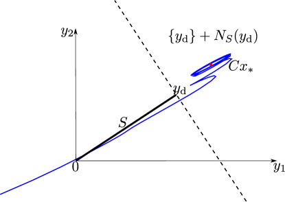
Figure 2: Trajectory of $Cx$ converging to interior of $\{y_{d}\}+N_{S}(y_{\mathrm{d}})$ with the multivalued control $u\in N_{S}(y)$ and $S=\operatorname{conv}\{0,y_{\mathrm{d}}\}$. This implies that $y$ converges to $y_{\mathrm{d}}$.

Remark 7.

From Figure 2 it is possible to see that, if $x_{*}$ satisfies the condition (3.6) for $y_{\mathrm{d}}\in S$, then we can achieve robust output regulation for any other desired value $\bar{y}_{\mathrm{d}}$ in the relative interior of $S$ by redefining the set $S$ to $\bar{S}=\operatorname{conv}\{0,\bar{y}_{\mathrm{d}}\}$. Moreover, in a more general setting, condition (3.6) allows us to attack the problem of robust tracking in the following way. Let $y_{\mathrm{d}}(t)$ be the desired reference signal. If, for all values of the function $y_{\mathrm{d}}:\mathbb{R}\to\mathbb{R}^{m}$, condition (3.6) is satisfied together with the bound in $\nu(t)$, then robust output tracking is possible as shown in Example 1 below.

Remark 8.

It is worth to note that a similar result can be obtained (with possibly different bounds in the external perturbation and different condition in $x_{*}$), if we change the form of the set $S$. For example, for $\Phi(y)=\psi_{S}(y)$ a possible set $S$ could be as the one given in Figure 3, where the point $y_{\mathrm{d}}$ is still in the boundary of $S$ and the normal cone to $S$ at $y_{\mathrm{d}}$ has no empty interior, the details are left to the reader.

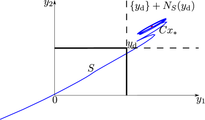
Figure 3: Trajectory $Cx$ converging to interior of $\{y_{d}\}+N_{S}(y_{\mathrm{d}})$ with the multivalued control $u\in N_{S}(y)$ and $S=\operatorname{conv}\{[0,0],[y_{\mathrm{d}_{1}},0],[0,y_{\mathrm{d}_{2}}],[y_{\mathrm{d}_{1}},y_{\mathrm{d}_{2}}]\}$.

4 Implementation issues and examples

4.1 Regularization

Up to this point, we have shown that whenever $u\in\partial\Phi(y)$ the membership of $y$ to the set $S$, together with robust output regulation are assured. Our next step is to develop a way to recover an explicit expression for the values of the control input $u$ in terms of the measured output $y$ and independent of the system parameters and state.

Note that exact values of input $u$ can be computed by solving the hemivariational inequality (2.8) at each time instant $t$, and making use of (3.3b), but this approach requires knowledge of the system parameters and state $x$.

As another alternative, it is worth noting that the approach of continuous selections does not yield the desired features. For example, in the case of $\varphi=0$, a continuous selection of the multifunction $\partial\Phi(\cdot)=N_{S}(\cdot)$ is $u=0$, (in fact $u=0$ is the unique continuous selection). However, with that control the storage function of (3.3) is given by $H_{1}$ with minimum at $\bar{x}$ and consequently, neither robust output regulation nor $y\in S$ properties are (in general) obtained. Similar results can be obtained when $\varphi\in\mathcal{C}^{1}$, since $u=\nabla\varphi(\cdot)$ is always a continuous selection of $\partial\Phi(\cdot)$.

Instead of looking for continuous selections of $\partial\Phi(\cdot)$, we are going to focus on a regularization of $\operatorname{Graph}\partial\Phi$ in the sense used in [14]. More precisely,

$$\tilde{u}-\nabla\varphi(y)\in N_{S}(y-\varepsilon\left[\tilde{u}-\nabla\varphi(y)\right])$$ (4.1)

is a regularization of the inclusion $u\in\partial\Phi(y)$. Namely, note that for $\varepsilon=0$ we recover $\tilde{u}\in\partial\Phi(y)$ (because $\partial\Phi(y)=\nabla\varphi(y)+N_{S}(y)$). Moreover, with the previous definition we are allowing outputs $y$ not necessarily in $S$. Instead we now require $y\in\{\varepsilon\left[\tilde{u}-\nabla\varphi(y)\right]\}+S$.

The well-posedness of inclusion (4.1) together with a single valued expression for $\tilde{u}$ are established below in Theorem 2. The following Lemma will be useful when proving it.

Lemma 3.

The map $f:\mathbb{R}^{m}\to\mathbb{R}^{m}$ given by

$$f(z):=(I+\varepsilon D^{-1})^{-1}z\;,$$

where $D^{-1}+D^{-T}>0$, is a contraction for all $\varepsilon>0$.

Proof.

Defining

$$\zeta=f(z)\;,$$

we have $(I+\varepsilon D^{-1})\zeta=z$ and direct computation gives

$$\|z_{1}-z_{2}\|^{2} =\left[(I+\varepsilon D^{-1})(\zeta_{1}-\zeta_{2})\right]^{\top}\left[(I+\varepsilon D^{-1})(\zeta_{1}-\zeta_{2})\right]$$

$$=\|\zeta_{1}-\zeta_{2}\|^{2}+\varepsilon(\zeta_{1}-\zeta_{2})^{\top}\left[D^{-1}+D^{-\top}\right](\zeta_{1}-\zeta_{2})$$

$$\>{}+\varepsilon^{2}(\zeta_{1}-\zeta_{2})^{\top}D^{-\top}D^{-1}(\zeta_{1}-\zeta_{2})$$

$$\geq\|\zeta_{1}-\zeta_{2}\|^{2}+\varepsilon\lambda_{\min}\left(D^{-1}+D^{-\top}\right)\|\zeta_{1}-\zeta_{2}\|^{2}$$

$$\>{}+\varepsilon^{2}\lambda_{\min}\left(D^{-\top}D^{-1}\right)\|\zeta_{1}-\zeta_{2}\|^{2}\;.$$

Therefore,

$$\|f(z_{1})-f(z_{2})\|\leq\dfrac{1}{\sqrt{1+\varepsilon\lambda_{\min}\left(D^{-1}+D^{-\top}\right)+\varepsilon^{2}\lambda_{\min}\left(D^{-\top}D^{-1}\right)}}\|z_{1}-z_{2}\|\;.$$

∎

Theorem 2.

Let $\varphi$ be a strictly convex, lower semicontinuous function that is $\mathcal{C}^{1}$ and satisfies

1. $\varphi(y)\geq\varphi(0)$ for all $y\in S$.

2. $\nabla\varphi:\mathbb{R}^{m}\to\mathbb{R}^{m}$ is Lipschitz continuous with constant $L$ such that

   $$L<\lambda_{\min}\left(\dfrac{D^{-1}+D^{-\top}}{2}\right)\;.$$

Then, for $\varepsilon>0$ sufficiently small, the regularized control $\tilde{u}$ can be expressed as:

$$\tilde{u}=\dfrac{y-\operatorname{Proj}_{S}(y)}{\varepsilon}+\nabla\varphi(y)$$ (4.2)

Furthermore, $\tilde{u}$ is passive respect to $y$.

Proof.

From (4.1) we have that for all $\sigma\in S$ the following holds:

$$0\geq\langle\tilde{u}-\nabla\varphi(y),\sigma-y+\varepsilon\left[\tilde{u}-\nabla\varphi(y)\right]\rangle\;.$$ (4.3)

Multiplying by $\varepsilon>0$ and adding and subtracting $y$ on the left-hand side of the inner product we obtain

$$0\geq\langle y-y+\varepsilon\left[\tilde{u}-\nabla\varphi(y)\right],\sigma-y+\varepsilon\left[\tilde{u}-\nabla\varphi(y)\right]\;.$$

Therefore,

$$y-\varepsilon\left[\tilde{u}-\nabla\varphi(y)\right]=\operatorname{Proj}_{S}(y)\;,$$

from which we obtain (4.2). Now we show that the interconnection of the plant (3.3a)–(3.3b) with the regularized control (4.2) is well-posed. It is easy to see that well-posedness of the closed-loop system is equivalent to proving that, for any state $x\in\mathbb{R}^{n}$, the equations

$$\tilde{u} =\dfrac{y-\operatorname{Proj}_{S}(y)}{\varepsilon}+\nabla\varphi(y),$$

$$\tilde{u} =D^{-1}\left(Cx-y\right),$$

have a unique solution. Proceeding with the substitution of the second equation and after some manipulations we have

$$y=\left(I+\varepsilon D^{-1}\right)^{-1}\left[\operatorname{Proj}_{S}(y)-\varepsilon\nabla\varphi(y)+\varepsilon D^{-1}Cx\right]=\left(f\circ g\right)\left(y\right)\;,$$

with $f$ as in Lemma 3 and $g:\mathbb{R}^{m}\to\mathbb{R}^{m}$ given by

$$g(z)=\operatorname{Proj}_{S}(z)-\varepsilon\nabla\varphi(z)+\varepsilon D^{-1}Cx\;.$$

We argue that the composition mapping $f\circ g$ is a contraction for $\varepsilon$ sufficiently small. Indeed, making use of Lemma 3 we have that

$$\big{\|}\left(f\circ g\right)\left(y_{1}\right)-\left(f\circ g\right)\left(y_{2}\right)\big{\|}\leq\dfrac{1}{\beta(\varepsilon)}\|g(y_{1})-g(y_{2})\|\leq\dfrac{1+\varepsilon L}{\beta(\varepsilon)}\|y_{1}-y_{2}\|$$

where $\beta(\varepsilon)=\left[1+\varepsilon\lambda_{\min}\left(D^{-1}+D^{-\top}\right)+\varepsilon^{2}\lambda_{\min}\left(D^{-\top}D^{-1}\right)\right]^{1/2}$. Note that the term $\frac{1+\varepsilon L}{\beta(\varepsilon)}$ is equal to $1$ for $\varepsilon=0$ and

$$\dfrac{d}{d\varepsilon}\left(\dfrac{1+\varepsilon L}{\beta(\varepsilon)}\right)\bigg{|}_{\varepsilon=0}=L-\lambda_{\min}\left(\dfrac{D^{-1}+D^{-\top}}{2}\right)<0\;,$$

i.e. the term $\frac{1+\varepsilon L}{\beta(\varepsilon)}$ is strictly decreasing in a neighbourhood of $\varepsilon=0$ and thus it is less than $1$ for $\varepsilon$ sufficiently small. Therefore, $f\circ g$ is a contraction and the interconnection is well-posed. It only rests to prove the passivity property of $\tilde{u}$. From (4.3) we have for $\sigma=0\in S$

$$\langle\tilde{u},y\rangle\geq\langle\nabla\varphi(y),y\rangle+\varepsilon\|\tilde{u}-\nabla\varphi(y)\|^{2}\;.$$

Note that for $\varepsilon=0$ we have $y\in S$ and from the strictly convexity assumption (see e.g. [10, p. 183]),

$$\langle\nabla\varphi(y),y\rangle>\varphi(y)-\varphi(0)\geq 0\text{ for all }y\in S\;.$$

In other words we have

$$\lim_{\varepsilon\downarrow 0}\langle\nabla\varphi(y),y\rangle+\varepsilon\|\tilde{u}-\nabla\varphi(y)\|^{2}>0\;.$$

Consequently, $\langle\tilde{u},y\rangle\geq 0$ for some $\varepsilon>0$ sufficiently small. ∎

Remark 9.

Note that Theorem 2 is still true if we change the first assumption by $\varphi(y)\geq\varphi(0)$ for all $y\in\operatorname{Dom}\varphi$ with $\varphi$ a convex function.

4.2 Example 1

Consider the circuit described by the diagram of Figure 4. We wish to regulate the outputs $y_{1}$ and $y_{2}$ to a desired value $y_{d}$.

Figure 4: Circuit diagram of Example 1, where the goal is to regulate the voltage at the outputs $y_{1}$ and $y_{2}$.

Taking as state variables the fluxes in inductors and charges in capacitors, we have the following state-space representation:

$$\dot{x} =\begin{bmatrix}-\frac{1}{R_{1}C_{1}}&-\frac{1}{L_{1}}&-\frac{1}{R_{1}C_{2}}&0\\ \frac{1}{C_{1}}&-\frac{R_{2}+R_{3}+R_{L_{1}}}{L_{1}}&0&\frac{R_{3}}{L_{2}}\\ -\frac{1}{R_{1}C_{1}}&0&-\frac{1}{R_{1}C_{2}}&-\frac{1}{L_{2}}\\ 0&\frac{R_{3}}{L_{1}}&\frac{1}{C_{2}}&-\frac{R_{3}+R_{L_{2}}}{L_{2}}\end{bmatrix}x+\begin{bmatrix}0&0\\ R_{L_{1}}&0\\ 0&0\\ 0&R_{L_{2}}\end{bmatrix}u+\begin{bmatrix}\frac{1}{R_{1}}\\ 0\\ \frac{1}{R_{1}}\\ 0\end{bmatrix}v$$ (4.4a)

$$y =\begin{bmatrix}0&\frac{R_{L_{1}}}{L_{1}}&0&0\\ 0&0&0&\frac{R_{L_{2}}}{L_{2}}\end{bmatrix}x+\begin{bmatrix}R_{L_{1}}&0\\ 0&R_{L_{2}}\end{bmatrix}u$$ (4.4b)

where $x=\begin{bmatrix}x_{1}&x_{2}&x_{3}&x_{4}\end{bmatrix}^{\top}$ are the charge in capacitor $C_{1}$, flux in inductor $L_{1}$, charge in capacitor $C_{2}$ and flux in inductor $L_{2}$, respectively, $u=\begin{bmatrix}u_{1}&u_{2}\end{bmatrix}^{\top}$ are the control inputs (currents) and $y=\begin{bmatrix}y_{1}&y_{2}\end{bmatrix}^{\top}$ are the voltages in resistances $R_{L_{1}}$ and $R_{L_{2}}$, respectively. Assume that we want to control the outputs to $y_{d}=\begin{bmatrix}1&f(t)\end{bmatrix}^{\top}$, where $f(t)$ is a sawtooth wave function with amplitude $0.5$ and frequency of $2$ Hz.

The system is passive because it is the result of the interconnection of passive elements. Values of system parameters are $R_{1}=R_{2}=R_{3}=1\Omega$, $R_{L_{1}}=2\Omega$, $R_{L_{2}}=3\Omega$, $L_{1}=1$H, $L_{2}=2$H, $C_{1}=1$F, $C_{2}=3$F, $v=10+50\sin(t)\operatorname{sign}(\sin(\pi t))$. Taking the convex function $\varphi=0$, simple algebra shows that condition (3.6) is equal to

$$\langle D^{-1}(y_{\mathrm{d}}-Cx_{*}),y_{\mathrm{d}}\rangle=-4-4f(t)+\dfrac{5}{6}f(t)^{2}\;,$$

which is negative for values of $f(t)\in(-0.849,5.649)$. The implemented control takes the form (4.2) with $\varepsilon=1\times 10^{-3}$ and $S$ the convex, time-varying set

$$S(t)=\operatorname{conv}\left\{\begin{bmatrix}0\\ 0\end{bmatrix},\begin{bmatrix}1\\ f(t)\end{bmatrix}\right\}\;.$$

Figure 5 shows the convergence of the output to the desired reference, even in the presence of the external perturbation $v$. Moreover, is easy to see that the condition $y\in S$ is satisfied. The computed control input is shown in Figure 6.

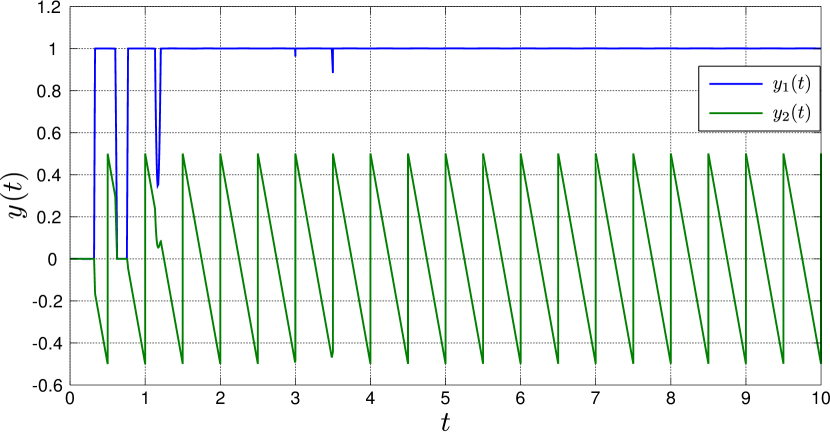
Figure 5: Output response of plant (4.4) with regularized control (4.2). The picture shows convergence to the desired output $y_{\mathrm{d}}$ (with $\varepsilon=1\times 10^{-3}$ and $\varphi=0$) subject to the perturbation $v(t)=10+50\sin(t)\operatorname{sign}(\sin(\pi t))$.

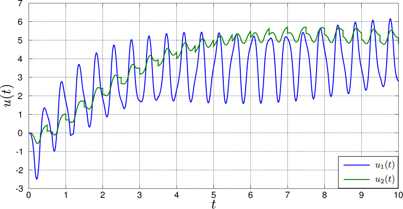
Figure 6: Time trajectory of regularized control (4.2) with $\varepsilon=1\times 10^{-3}$ and $\varphi=0$.

4.3 Example 2

Consider the following affine system

$$\dot{x} =Ax+B_{\mathrm{u}}u_{1}+B_{\mathrm{v}}v$$ (4.5a)

$$y_{1} =Cx+Du_{1}$$ (4.5b)

with

$$A =\begin{bmatrix}-3.7036&1.9043&-0.9735&0.4164\\ -0.2421&-5.1187&-0.0478&0.0269\\ -0.9915&-1.0461&-5.5232&-0.5318\\ 0.4376&2.1467&-0.5948&-3.6545\end{bmatrix}, B_{\mathrm{u}}= \begin{bmatrix}-0.6918&-1.4410\\ 0.8580&0.5711\\ 1.2540&-0.3999\\ -1.5937&0.6900\end{bmatrix},$$

$$C =\begin{bmatrix}0.0652&0.4889&0.6820&0.9166\\ 0.7134&0.6677&0.1996&0.8659\end{bmatrix}, B_{\mathrm{v}}= \begin{bmatrix}0.8147&1.4345\\ 0.9058&2.5464\\ -0.1270&0\\ 0.9134&-1.0453\\ \end{bmatrix},$$

$$D =\begin{bmatrix}1.0823&0.3899\\ -0.1315&0.088\end{bmatrix}\;.$$

where the external perturbation signal $v(t)$ is decomposed as

$$v(t)=\begin{bmatrix}4\\ 0\end{bmatrix}+\begin{bmatrix}f_{1}(t)\\ f_{2}(t)\end{bmatrix}$$ (4.6)

with $f_{1}(t)$ a sinusoidal function with amplitude $2$ and frequency of 10 Hz and $f_{2}(t)$ corresponds to a sawtooth wave with amplitude $3$ and frequency of $\pi$ Hz. Suppose that we want to regulate the output to the set-point $y_{\mathrm{d}}=\begin{bmatrix}-1&2\end{bmatrix}$.

Let us verify the assumptions of Theorem 1. The equilibrium point $x_{*}$ is

$$x_{*}=\begin{bmatrix}2.7809&0.1184&-0.2779&0.4877\end{bmatrix}^{\top}\;.$$

and it satisfies

$$\langle D^{-1}(y_{\mathrm{d}}-Cx_{*}),y_{\mathrm{d}}\rangle=-9.2810\;.$$

Taking, for example, the convex function $\varphi(y)=\log\left(e^{y_{1}}+e^{y_{2}}\right)$, which is proper and $\mathcal{C}^{1}$, we have that

$$\mathcal{D}\varphi(y_{\mathrm{d}},-y_{\mathrm{d}})=-\langle\nabla\varphi(y_{\mathrm{d}}),y_{\mathrm{d}}\rangle=-1.8577\;.$$

Condition (3.6) is satisfied. Using the SDPT3 software to solve (2.2) we obtain

$$P=\begin{bmatrix}1.8765&1.8706&-0.5249&1.3338\\ 1.8706&3.8984&-0.4599&0.9207\\ -0.5249&-0.4599&2.4211&0.4920\\ 1.3338&0.9207&0.4920&2.0056\end{bmatrix}\;,$$

which is positive definite with eigenvalues in $\{0.2296,1.5399,2.7431,5.6889\}$. Figure 7 shows the output response for a regularized control $\tilde{u}$ with $\varepsilon=1\times 10^{-4}$, where finite time convergence toward the desired set-point can be verified despite the external parametric disturbances of the system. Control and state trajectories are shown in Figures 8 and 9, respectively.

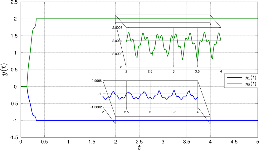
Figure 7: Output’s time trajectory for plant (4.5) showing the convergence to the desired value $y_{\mathrm{d}}=[-1\quad 2]^{\top}$.

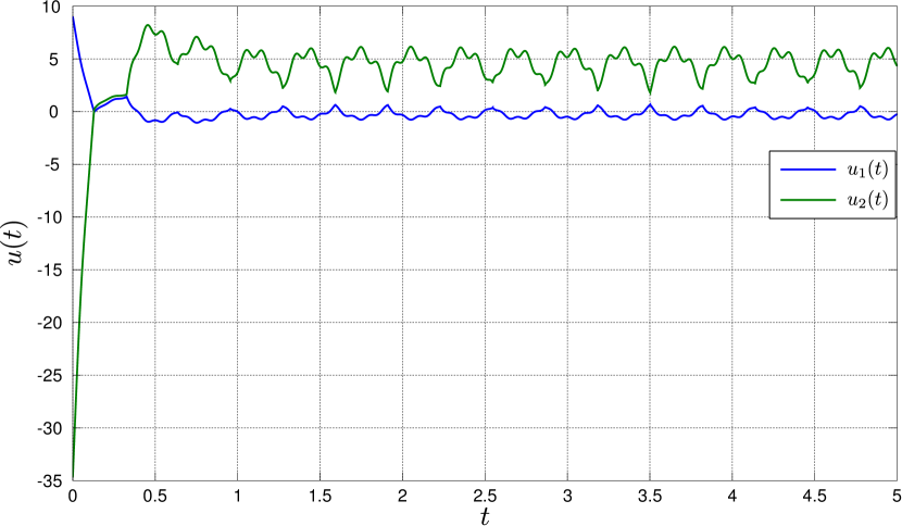
Figure 8: Time trajectory of regularized control (4.2) applied to the plant (4.5) with $\varepsilon=1\times 10^{-4}$ and $\varphi=\log(e^{y_{1}}+e^{y_{2}})$.

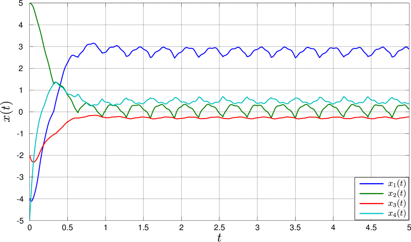
Figure 9: State’s time trajectories of regulated plant (4.5) with the regularized control (4.2) (with $\varepsilon=1\times 10^{-4}$ and $\varphi=\log(e^{y_{1}}+e^{y_{2}})$) and perturbation (4.6).

5 Conclusions

This note presents an extension (for the $m$-dimensional case) of the multivalued control presented in [14]. Moreover, more general multivalued functions of the form $u\in\partial\Phi(y)$ are considered, assuring finite time convergence together with, robust output regulation in the face of parametric and external (bounded) disturbances.

The effect of the multivalued control relies directly on the dissipation term modifying the rate of convergence of the storage function $H_{2}$ to $x_{*}$ and leaving without change the interconnection matrix $J$.

Between the main assumptions considered, the fact that $D$ is invertible plays an essential role. A research line is the case of no $D$ (i.e. $y=Cx$).

The implemented control (4.2) acts in fact as a high gain controller when $y\notin S$ and coincides with the continuous selection of $\partial\Phi(y)$ when $y\in S$. However, since the output contains a feedthrough component of the input, the high gain does not result in arbitrary large controls. That is, the control converges to a bounded, well-defined value as $\varepsilon\to 0$. It is worth noting that the resulting controller is passive and independent of the system parameters and of the system state.

The well-suited structure of Port-Hamiltonian systems together with passivity opens the opportunity to investigate the robust output regulation problem in the nonlinear setting.

References

- [1] V. Acary and B. Brogliato. Numerical Methods for Nonsmooth Dynamical Systems. Springer-Verlag, Berlin, 2008.
- [2] B. Brogliato. Absolute stability and the lagrange–dirichlet theorem with monotone multivalued mappings. Systems and Control Letters, 51(5):343 – 353, 2004.
- [3] B. Brogliato, A. Daniilidis, C. Lemaréchal, and V. Acary. On the equivalence between complementarity systems, projected systems and differential inclusions. Systems and Control Letters, 55(1):45 – 51, 2006.
- [4] B. Brogliato and D. Goeleven. Well-posedness, stability and invariance results for a class of multivalued lur’e dynamical systems. Nonlinear Analysis: Theory, Methods and Applications, 74(1):195 – 212, 2011.
- [5] B. Brogliato and D. Goeleven. Existence, uniqueness of solutions and stability of nonsmooth multivalued Lur’e dynamical systems. Journal of Convex Analysis, 20(3):881–900, 2013.
- [6] F. Castaños and R. Ortega. Energy-balancing passivity-based control is equivalent to dissipation and output invariance. Systems & Control Letters, 58(8):553–560, August 2009.
- [7] F. Facchinei and J.S. Pang. Finite-Dimensional Variational Inequalities and Complementarity Problems. Number V. 1 in Finite-dimensional Variational Inequalities and Complementarity Problems. Springer, 2003.
- [8] A.F. Filippov and F.M. Arscott. Differential Equations with Discontinuous Righthand Sides: Control Systems. Mathematics and its Applications. Springer, 1988.
- [9] D. Goeleven, D. Motreanu, Y. Dumont, and M. Rochdi. Variational and Hemivariational Inequalities - Theory, Methods and Applications: Volume I: Unilateral Analysis and Unilateral Mechanics. Nonconvex Optimization and Its Applications. Springer, 2003.
- [10] J. B. Hiriart-Urruty and C. Lemaréchal. Convex Analysis and Minimization Algorithms I. Springer-Verlag, New York, 1993.
- [11] H.K. Khalil. Nonlinear Systems. Prentice Hall, third edition, 2002.
- [12] L. Knockaert. A note on strict passivity. Systems & Control Letters, 54(9):865–869, September 2005.
- [13] R. I. Leine and N. van der Wouw. Stability and Convergence of Mechanical Systems with Unilateral Constraints. Springer-Verlag, Berlin, 2008.
- [14] F.A Miranda and F. Castaños. Robust output regulation of variable structure systems with multivalued controls. In Variable Structure Systems (VSS), 2014 13th International Workshop on, pages 1–6, June 2014.
- [15] A. Nagurney and D. Zhang. Projected Dynamical Systems and Variational Inequalities with Applications. Innovations in Financial Markets and Institutions. Springer US, 1995.
- [16] R. Ortega, A. Loría, P. J. Nicklasoon, and H. Sira-Ramírez. Passivity-based Control of Euler-Lagrange Systems: Mechanical, Electrical and Electromechanical Applications. Communications and Control Engineering. Springer, 1998.
- [17] R. Ortega, A. van der Schaft, B. Maschke, and G. Escobar. Interconnection and damping assignment passivity-based control of port-controlled Hamiltonian systems. Automatica, 38(4):585–596, April 2002.
- [18] R.T. Rockafellar. Convex Analysis. Convex Analysis. Princeton University Press, 1970.
- [19] V.I. Utkin. Sliding Modes in Control and Optimization. Communications and Control Engineering. Springer-Verlag, 1992.
- [20] A.J. Van der Schaft. L2-Gain and Passivity Techniques in Nonlinear Control. Lecture Notes in Control and Information Sciences. Springer, 1996.
- [21] J. C. Willems. On interconnections, control, and feedback. Automatic Control, IEEE Transactions on, 42(3):326 – 339, March 1997.
- [22] M.K. Çamlıbel, W.P.M.H. Heemels, and J.M. Schumacher. On linear passive complementarity systems. European Journal of Control, 8(3):220 – 237, 2002.