Intrinsic Physical Conditions and Structure of Relativistic Jets in Active Galactic Nuclei

Abstract

The analysis of the frequency dependence of the observed shift of the cores of relativistic jets in active galactic nuclei (AGN) allows us to evaluate the number density of the outflowing plasma $n_{\mathrm{e}}$ and, hence, the multiplicity parameter $\lambda=n_{\mathrm{e}}/n_{\mathrm{GJ}}$, where $n_{\mathrm{GJ}}$ is the Goldreich-Julian number density. We have obtained the median value for $\lambda_{\mathrm{med}}=3\cdot 10^{13}$ and the median value for the Michel magnetization parameter $\sigma_{\mathrm{M,med}}=8$ from an analysis of 97 sources. Since the magnetization parameter can be interpreted as the maximum possible Lorentz factor $\Gamma$ of the bulk motion which can be obtained for relativistic magnetohydrodynamic (MHD) flow, this estimate is in agreement with the observed superluminal motion of bright features in AGN jets. Moreover, knowing these key parameters, one can determine the transverse structure of the flow. We show that the poloidal magnetic field and particle number density are much larger in the center of the jet than near the jet boundary. The MHD model can also explain the typical observed level of jet acceleration. Finally, casual connectivity of strongly collimated jets is discussed.

1 Introduction

Strongly collimated jets represent one of the most visible signs of the activity of compact astrophysical sources. They are observed both in relativistic objects such as active galactic nuclei (AGNs) and microquasars, and in young stars where the motion of matter is definitely nonrelativistic. This implies that we are dealing with some universal and extremely efficient mechanism of energy release.

At present the magnetohydrodynamic (MHD) model of activity of compact objects is accepted by most astrophysicists (Mestel, 1999; Krolik, 1999). At the heart of the MHD approach lies the model of the unipolar inductor, i.e., a rotating source of direct current. It is believed that the electromagnetic energy flux — the Poynting flux — plays the main role in the energy transfer from the ‘central engine’ to active regions. The conditions for the existence of such a ‘central engine’ are satisfied in all the compact sources mentioned above. Indeed, all compact sources are assumed to harbor a rapidly spinning central body (black hole, neutron star, or young star) and some regular magnetic field, which leads to the emergence of strong induction electric fields. The electric fields, in turn, lead to the appearance of longitudinal electric currents resulting in effective energy losses and particle acceleration.

The first studies of the electromagnetic model of compact sources (namely, radio pulsars) were carried out as early as the end of the 1960s (Goldreich & Julian, 1969; Michel, 1969). It was evidenced that there are objects in the Universe in which electrodynamical processes can play the decisive role in the energy release. Then, Blandford (1976) and Lovelace (1976) independently suggested that the same mechanism can also operate in active galactic nuclei, and for nearly 40 years this model has remained the leading one.

Remember that within the MHD approach the total energy losses $P_{\rm jet}$ can be easily evaluated as $P_{\rm jet}\sim IU$, where $I$ is the total electric current flowing along the jet, and $U\sim ER_{0}$ is the electro-motive force exerted on the black hole on the scale $R_{0}$. If the central engine (black hole for AGNs) rotates withthe angular velocity $\Omega$ in the external magnetic field $B_{0}$, one can evaluate the electric field as $E\sim(\Omega R_{0}/c)B_{0}$. On the other hand, assuming that for AGNs the current density $j$ is fully determined by the relativistic outflow of the Goldreich-Julian charge density $\rho_{\rm GJ}=\Omega B_{0}/(2\pi c)$ (i.e., the minimum charge density required for the screening of the longitudinal electric field in the magnetosphere), one can write down $j\approx c\rho_{\rm GJ}$. It gives

$$I\sim\Omega B_{0}R_{0}^{2}.$$ (1)

As for AGNs, one can set $R_{0}\approx r_{\rm g}=2GM/c^{2}$ to obtain the well-known evaluation (Blandford & Znajek, 1977)

$$P_{\rm jet}\sim\left(\frac{\Omega r_{\rm g}}{c}\right)^{2}B_{0}^{2}r_{\rm g}^{2}c.$$ (2)

In particular, comparing expressions (1) and (2), one can straightforwardly obtain

$$I\approx c^{1/2}P_{\rm jet}^{1/2}.$$ (3)

For AGNs it corresponds to $10^{19}$–$10^{21}$ A. Certainly, the question as to whether it is possible to consider a black hole immersed in an external magnetic field as a unipolar inductor turned out to be also rather nontrivial (Punsly, 2001; Okamoto, 2009; Beskin, 2009).

As a result, the MHD model was successfully used to describe a lot of processes in active nuclei including the problem of the stability of jets (Benford, 1981; Hardee & Norman, 1988; Appl & Camenzind, 1992; Istomin & Pariev, 1994; Bisnovatyi-Kogan, 2007; Lyubarsky, 2009) and their synchrotron radiation (Blandford & Königl, 1977; Pariev, Istomin & Beresnyak, 2003; Lyutikov, Pariev & Gabuzda, 2005). In particular, it was shown both analytically (Bogovalov, 1995; Heyvaerts & Norman, 2003; Beskin & Nokhrina, 2009) and numerically (Komissarov et al., 2006; Tchekhovskoy et al., 2009; Porth et al., 2011; McKinney et al., 2012) that for sufficiently small ambient pressure the dense core can be formed. This is related both to advances in the theory which have at last formulated sufficiently simple analytical relations (Blandford & Znajek, 1977; Beskin, 2010), and to the breakthrough in numerical simulations (Komissarov et al., 2006; Tchekhovskoy et al., 2009; Porth et al., 2011; McKinney et al., 2012) which confirmed theoretical predictions.

Moreover, recently Kronberg et al. (2011) demonstrated that in QSO 3C303 the jet does possess large enough toroidal magnetic field, the apropriate longitudinal electric current along the jet $I\approx 1.7\times 10^{19}$ A being as large as the electric current $I_{\rm GJ}$ (Eq. 1) which is necessary to support the Poynting energy flux. Besides, the lack of $\gamma$-ray radiation as probed by the Fermi Observatory for AGN jets observed at small enough viewing angles $\vartheta<5^{\circ}$ (Savolainen et al., 2010) can be easily explained as well. Indeed, as was found (see, e.g., Beskin 2010), within well-collimated magnetically dominated MHD jets the Lorentz factors of the particle bulk motion can be evaluated as

$$\Gamma\approx r_{\perp}/R_{\rm L},$$ (4)

where $r_{\perp}$ is the distance from the jet axis, and $R_{\rm L}=c/\Omega$ is the light cylinder radius. Thus, the energy of particles radiating in small enough angles $\vartheta$ with respect to the jet axis is to be much smaller than that corresponding to peripheral parts of a jet.

The most important MHD parameters describing relativistic flows (which was originally introduced for radio pulsars) are the Michel magnetization parameter $\sigma_{\rm M}$ and the multiplicity parameter $\lambda$. The first one determines the maximum possible bulk Lorentz factor $\Gamma$ of the flow when all the energy transported by the Poynting flux is transmitted to particles. The second one is the dimensionless multiplicity parameter $\lambda=n_{\rm e}/n_{\rm GJ}$, which is defined as the ratio of the number density $n_{\rm e}$ to the Goldrech-Julian (GJ) number density $n_{\rm GJ}=\Omega B/2\pi ce$. It is important that these two parameters are connected by the simple relation (Beskin, 2010)

$$\sigma_{\rm M}\approx\frac{1}{\lambda}\left(\frac{P_{\rm jet}}{P_{\rm A}}\right)^{1/2}.$$ (5)

Here $P_{\rm A}=m^{2}c^{5}/e^{2}\approx 10^{17}$ erg/s is the minimum energy losses of the central engine which can accelerate particles to relativistic energies, and $P_{\rm jet}$ is the total energy losses of the compact object.

Unfortunately, up to now neither the magnetization nor the multiplicity parameters were actually known as the observations could not give us the direct information about the number density and bulk energy of particles. The core shift method has been applied to obtain the concentration $n_{\rm e}$, magnetic field $B$ (Lobanov, 1998; O’Sullivan & Gabuzda, 2009; Pushkarev et al., 2012; Zdziarski et al., 2014), and the jet composition (Hirotani, 2005) in AGN jets. However, evaluation of multiplicity and Michel magnetization parameters, which needs to estimate the total jet power, has not been done. From a theoretical point of view if the inner parts of the accretiondisc are hot enough, then electron-positron pairs can be produced by two-photon collisions,where photons with sufficient energy originate from the inner parts of the accretion disk (Blandford & Znajek, 1977; Moscibrodzka et al., 2011). In this case $\lambda\sim 10^{10}$–$10^{13}$, and Michel magnetization parameter $\sigma_{\rm M}\sim 10$–$10^{3}$. The second model takes into account the appearance of the region where the GJ plasma density is equal to zero due to general relativity effects that corresponds to the outer gap in the pulsar magnetosphere (Beskin, Istomin & Pariev, 1992; Hirotani & Okamoto, 1998). This model gives $\lambda\sim 10^{2}$–$10^{3}$, and $\sigma_{\rm M}\sim 10^{10}$–$10^{13}$.

This large difference in the estimates for the magnetization parameter $\sigma_{\rm M}$ leads to two completely different pictures of the flow structure in jets. In particular, it determines whether the flow is magnetically or particle dominated. The point is that for ordinary jets $r_{\perp}/R_{\rm L}\sim 10^{4}$–$10^{5}$. As a result, using the universal asymptotic solution $\Gamma\approx r_{\perp}/R_{\rm L}$ (4), one can obtain that the values $\sigma_{\rm M}\sim 10$–$10^{3}$ correspond to the saturation regime when almost all the Poynting flux $W_{\rm em}$ is transmitted to the particle kinetic energy flux $W_{\rm part}$. On the other hand, for $\sigma_{\rm M}\sim 10^{12}$ the jet remains magnetically dominated ($W_{\rm part}\ll W_{\rm em}$). Thus, the determination of Michel magnetization parameter $\sigma_{\rm M}$ is the key point in the analysis of the internal structure of relativistic jets.

The paper is organized as follows. In section 2 it is shown that VLBI observations of synchrotron self-absorbtion in AGN jets allow us to evaluate the number density of the outflowing plasma $n_{\rm e}$ and, hence, the multiplicity parameter $\lambda$. We discuss the source sample and present the result for multiplicity and Michel magnetization mparameters in section 3. The values $\lambda\sim 10^{13}$ obtained from the analysis of 97 sources shows that for most jets the magnetization parameter $\sigma_{\rm M}\lesssim 30$. Since the magnetization parameter is the maximum possible value of the Lorentz factor of the relativistic bulk flow, this estimate is consistent with observed superluminal motion.In section 4 it is shown that for physical parameters determined above, the poloidal magnetic field and particle number density are much larger in the center of the jet than near its boundary. Finally, in section 5 the casual connectivity of strongly collimated supersonic jets is discussed. Throughout the paper, we use the $\Lambda$CDM cosmological model with $H_{0}=71$ km s^-1 Mpc^-1, $\Omega_{m}=0.27$, and $\Omega_{\Lambda}=0.73$ (Komatsu et al., 2009).

2 The method

2.1 General relations

To determine the multiplicity parameter $\lambda$ and Michel magnetization parameter $\sigma_{\rm M}$ one can use the dependence on the visible position of the core of the jet from the observation frequency (Gould, 1979; Blandford & Königl, 1977; Marscher, 1983; Lobanov, 1998; Hirotani, 2005; Kovalev et al., 2008; O’Sullivan & Gabuzda, 2009; Sokolovsky et al., 2011; Pushkarev et al., 2012). This effect is associated with the absorption of the synchrotron photon gas by relativistic electrons (positrons) in a jet.

Typically, the parsec-scale radio morphology of a bright AGN manifests a one-sided jet structure due to Doppler boosting that enhances the emission of the approaching jet. The apparent base of the jet is commonly called the “core”, and it is often the brightest and most compact feature in VLBI images of AGN. The VLBI core is thought to represent the jet region where the optical depth is equal to unity.

We will employ the following model to connect the physical parameters at the jet launching region with the observable core-shift. There is a magnetohydrodynamic relativistic outflow of non-emitting plasma moving with bulk Lorentz factor $\Gamma$ and concentration $n_{\rm e}$ in the observer rest frame. On the latter we superimpose the flow of emitting particles with distribution ${\rm d}n_{{\rm syn}*}=k_{{\rm e}*}\gamma_{*}^{-1+2\alpha}{\rm d}\gamma_{*}$, $\gamma_{*}\in[\gamma_{\rm min*};\;\gamma_{\rm max*}]$. Here $n_{\rm syn*}$ is concentration of emitting plasma, $k_{\rm e*}$ is concentration aplitude, and $\gamma_{*}$ is the emitting particles’ Lorentz factor. All the parameters with subscript ‘*’ are taken in the non-emitting plasma rest frame, i.e., in the frame which locally moves with the bulk Lorentz factor $\Gamma$.

We suppose that the emitting particles radiate synchrotron photons in the jet’s magnetic field, and these photons scatter off the same electrons, which lead to the photon absorption (Gould, 1979; Lobanov, 1998; Hirotani, 2005). The corresponding turn-over frequency $\nu_{\mathrm{m*}}$, the frequency at which the flux density $S_{\nu}$ has a maximum, can be evaluated using expressions from Gould (1979) as

$$\nu_{\mathrm{m*}}^{(5-2\alpha)}=\frac{c_{\alpha}^{2}(1-2\alpha)}{5(5-2\alpha)}\frac{e^{4}}{m^{2}c^{2}}\left(\frac{e}{2\pi mc}\right)^{3-2\alpha}R_{*}^{2}B_{*}^{3-2\alpha}k_{\rm e*}^{2}.$$ (6)

The function $c_{\alpha}\,(\cdot)$ is a composition of gamma-functions defined by Gould (1979), and for $\alpha=-1/2$ we have $c_{\alpha}\,(2)=1.396$. Constants $e$, $m$, and $c$ are the electron charge, electron mass, and the speed of light correspondingly. Finally, $B_{*}$ is the magnitude of disordered magnetic field in an emitting region with a characteristic size $R_{*}$ along the line of sight.

Although we assume that the toroidal magnetic field dominates in the jet, an assumption of disordered magnetic field in our opinion can be retained, because, for an optically thin jet, the photon meets both directions of field. Thus, the mean magnetic field along the photon path is almost zero, which mimics the behaviour of a disordered field. As a result, the parameters in the observer rest frame and plasma rest frame are connected by the following equations:

$$\frac{\nu_{\rm m*}}{\nu_{\rm m}}=\frac{1+z}{\delta},$$ (7)

$$R_{*}=\frac{2\,r_{*}\chi_{*}}{\sin{\varphi_{*}}}=\frac{2\,r\chi}{\delta\sin{\varphi}},$$ (8)

$$B_{*}=\sqrt{B^{2}-E^{2}}\approx\frac{B_{\varphi}}{\Gamma}\approx\frac{B}{\Gamma},$$ (9)

$$k_{\rm e*}=\frac{k_{\rm e}}{\Gamma},$$ (10)

where $z$ is the red-shift,

$$\delta=\frac{1}{\Gamma\left(1-\beta\cos\varphi\right)}$$ (11)

is the Doppler factor, $\chi$ is the jet half-opening angle, and $\varphi$ is a viewing angle.

Further, the number density of emitting electrons $n_{\rm syn}$ is connected with the amplitude $k_{\rm e}$ as

$$k_{\rm e}=n_{\rm syn}\frac{2\alpha}{\gamma_{\rm max}^{2\alpha}-\gamma_{\rm min}^{2\alpha}},$$ (12)

where $\gamma=\gamma_{*}\Gamma$. For $\alpha=-1/2$ we get

$$k_{\rm e}\approx n_{\rm syn}\gamma_{\rm min}.$$ (13)

We also put $n_{\rm syn}=\xi n_{\rm e}$. Here $\xi$ is a ratio of the number density of emitting particles to the MHD flow number density. The portion of particles effectively accelerated by the internal shocks was found by Sironi, Spitkovsky & Arons (2013) to be about 1%, so we take $\xi\approx 0.01$.

Finally, we assume (Lobanov, 1998; Hirotani, 2005) the following power law behavior for the magnetic field and particle density dependence on distance:

$$B(r)=B_{1}\left(\frac{r}{r_{1}}\right)^{-1},$$ (14)

$$n_{\rm e}(r)=n_{1}\left(\frac{r}{r_{1}}\right)^{-2},$$ (15)

where $B_{1}$ is the magnetic field and $n_{1}$ is the number density at $r_{1}=1$ pc respectively. For these scalings of particle density and magnetic field with the distance the turn-over frequency $\nu_{\rm m}$ as a function of $r$ does not depend on $\alpha$ and can be written as

$$\nu_{\rm m}\propto r^{-1}.$$ (16)

This scaling has been confirmed by Sokolovsky et al. (2011) in measurements of core-shifts for 20 AGNs made for 9 frequencies each. Using these dependencies of magnetic field and particle number density of distance $r$, we obtain in the observer rest frame

$$\begin{array}[]{l}\displaystyle\left(\nu_{\rm m}\frac{1+z}{\delta}\frac{r}{r_{1}}\right)^{5-2\alpha}=C\left(\frac{2e^{2}}{mc}\right)^{2}\left(\frac{e}{2\pi mc}\right)^{3-2\alpha}\times\\ \displaystyle\times\left(\frac{r_{1}\chi}{\delta\sin\varphi}\,\xi\gamma_{\rm min}\right)^{2}\Gamma^{-5+2\alpha}B_{1}^{3-2\alpha}n_{1}^{2},\end{array}$$ (17)

where $C=c_{\alpha}^{2}(1-2\alpha)/5(5-2\alpha)$.

On the other hand, the values $B_{1}$ and $n_{1}$ can be related through introducing the flow magnetization parameter $\sigma$ — the ratio of Poynting vector to particle kinetic energy flux at a given distance along the flow (see Appendix A). Let us define the magnetization $\sigma_{\xi}$ as a ratio of Poynting vector to the total kinetic energy flux of emitting and non-emitting particles:

$$\sigma_{\xi}=\frac{\left|\vec{S}\right|}{\left|\vec{K}+\vec{K}_{\rm syn}\right|}.$$ (18)

Here the kinetic energy flux of emitting electrons is

$$\left|\vec{K}_{\rm syn}\right|=\int_{\gamma_{\rm min}}^{\gamma_{\rm max}}(\gamma mc^{2})(|\vec{v}_{\rm p}|){\rm d}n_{\rm syn}=k_{\rm e}mc^{3}F(\gamma_{\rm min},\gamma_{\rm max}),$$ (19)

and function $F\,(\cdot)$ for $\alpha=-1/2$ is defined by the following expression:

$$\begin{array}[]{l}\displaystyle F(\gamma_{\rm min},\gamma_{\rm max})=\left({\rm ch}^{-1}\gamma_{\rm max}-{\rm ch}^{-1}\gamma_{\rm min}\right)-\\ \\ \displaystyle-\left(\frac{\sqrt{\gamma^{2}_{\rm max}-1}}{\gamma_{\rm max}}-\frac{\sqrt{\gamma^{2}_{\rm min}-1}}{\gamma_{\rm min}}\right)\approx\ln\left(2\gamma_{\rm max}\right)-1.\end{array}$$ (20)

Estimating now the Poynting vector as

$$\left|\vec{S}\right|\approx\frac{cB^{2}_{\varphi}}{4\pi},$$ (21)

and particle kinetic energy fluxes as

$$\left|\vec{K}+\vec{K}_{\rm syn}\right|\approx mc^{3}n_{\rm e}\left(\Gamma+\xi F\gamma_{\rm min}\right),$$ (22)

we obtain the following relationship between magnetic field and particle number density:

$$B^{2}=\sigma_{\xi}4\pi mc^{2}n_{\rm e}\Gamma.$$ (23)

In what follows, we neglect the term $\xi F\gamma_{\rm min}$ in comparison with $\Gamma$. Further on we omit the index $\xi$. Using (23), we get

$$\begin{array}[]{l}\displaystyle\left(\nu_{\rm m}\frac{1+z}{\delta}\frac{r}{r_{1}}\right)^{5-2\alpha}=C\left(\frac{2e^{2}}{mc}\right)^{2}\left(\frac{e}{2\pi mc}\right)^{3-2\alpha}\times\\ \\ \displaystyle\times\left(4\pi mc^{2}\right)^{1.5-\alpha}\left(\frac{r_{1}\chi}{\delta\sin\varphi}\,\xi\gamma_{\rm min}\right)^{2}\Gamma^{-5+2\alpha}\times\\ \\ \displaystyle\times\left(\sigma_{1}\Gamma_{1}\right)^{1.5-\alpha}n_{1}^{3.5-\alpha}.\end{array}$$ (24)

As to the number density $n_{1}$, it can be defined through the multiplicity parameter $\lambda$ and total jet energy losses $P_{\rm jet}$ as (see Appendix B for more detail)

$$n_{1}=\frac{\lambda}{2\pi\left(r_{1}\chi\right)^{2}}\frac{mc^{2}}{e^{2}}\sqrt{\frac{P_{\rm jet}}{P_{\rm A}}}.$$ (25)

2.2 The saturation regime

To determine the intrinsic parameters of relativistic jets, let us consider two cases for the different magnetization at 1 pc. In what follows we assume that the flow at its base is highly, or at least mildly, magnetized, i.e. $\sigma_{\rm M}\gg 1$.

First, we assume that up to the distance $r=1$ pc the plasma has been effectivily accelerated so that the Poynting flux is smaller in comparison with the particle kinetic energy flux, i.e., $\sigma_{1}\lesssim 1$. In other words, the acceleration reached the saturation regime (Beskin, 2010). Combining now (4) and (55), it is easy to obtain that this case corresponds to $\sigma_{\rm M}<10^{5}$. Accordingly, the bulk Lorentz factor at $r=1$ pc can be evaluated as

$$\Gamma_{1}\approx\sigma_{\rm M}.$$ (26)

In this case Eqn. (24) can be rewritten as

$$\left(\nu_{\rm m}\frac{1+z}{\delta}\frac{r\chi}{c}\right)^{5-2\alpha}=C\left(\frac{2^{-1.5+\alpha}}{\pi^{5-2\alpha}}\right)\left(\frac{\xi\gamma_{\rm min}}{\delta\sin\varphi}\right)^{2}\lambda^{7-2\alpha}.$$ (27)

Using now the relationship between the angular distance $\theta_{\rm d}$ and the distance from the jet base $r$

$$r\sin\varphi=\theta_{\rm d}\frac{D_{\rm L}}{(1+z)^{2}},$$ (28)

where $D_{\rm L}$ is the luminosity distance, we obtain

$$\begin{array}[]{l}\displaystyle\left(\frac{\theta_{\rm d}}{\rm mas}\right)=3.4\cdot 10^{-19}\left(\frac{D_{\rm L}}{\rm Gpc}\right)^{-1}\left(\frac{\nu_{\rm m}}{\rm GHz}\right)^{-1}{\delta(1+z)}\times\\ \\ \displaystyle\times\frac{\sin\varphi}{\chi}\left(\frac{\xi\gamma_{\rm min}}{\delta\sin\varphi}\right)^{2/(5-2\alpha)}\lambda^{(7-2\alpha)/(5-2\alpha)}.\end{array}$$ (29)

This expression can be rewritten as a following relationship between the core position and the observation frequency:

$$\left(\frac{\theta_{\rm d}}{\rm mas}\right)=\left(\frac{\eta}{\rm mas\cdot GHz}\right)\left(\frac{\nu_{\rm m}}{\rm GHz}\right)^{-1}.$$ (30)

Having the measured core-shift $\Delta r_{\rm mas}$ in milliarcseconds for two frequencies $\nu_{\rm m,1}$ and $\nu_{\rm m,2}$, we obtain for $\alpha=-1/2$:

$$\begin{array}[]{l}\displaystyle\lambda=7.3\cdot 10^{13}\left(\frac{\eta}{\rm mas\cdot GHz}\right)^{3/4}\left(\frac{D_{\rm L}}{\rm Gpc}\right)^{3/4}\times\\ \\ \displaystyle\times\left(\frac{\chi}{1+z}\right)^{3/4}\frac{1}{(\delta\sin\varphi)^{1/2}}\frac{1}{(\xi\gamma_{\rm min})^{1/4}}=\\ \\ \displaystyle=2.3\cdot 10^{14}\left(\frac{\eta}{\rm pc\cdot GHz}\right)^{3/4}\left(\frac{D_{\rm L}}{\rm Gpc}\right)^{3/4}\times\\ \\ \displaystyle\times\left(\frac{\chi}{1+z}\right)^{3/4}\frac{1}{(\delta\sin\varphi)^{1/2}}\frac{1}{(\xi\gamma_{\rm min})^{1/4}}.\end{array}$$ (31)

Accordingly, using (5), we obtain

$$\begin{array}[]{l}\displaystyle\sigma_{\rm M}=1.4\cdot\left[\left(\frac{\eta}{\rm mas\cdot GHz}\right)\left(\frac{D_{\rm L}}{\rm Gpc}\right)\frac{\chi}{1+z}\right]^{-3/4}\times\\ \\ \displaystyle\times\sqrt{\delta\sin\varphi}\left(\xi\gamma_{\rm min}\right)^{1/4}\sqrt{\frac{P_{\rm jet}}{10^{45}{\rm erg\cdot s^{-1}}}}=\\ \\ \displaystyle=0.44\cdot\left[\left(\frac{\eta}{\rm pc\cdot GHz}\right)\left(\frac{D_{\rm L}}{\rm Gpc}\right)\frac{\chi}{1+z}\right]^{-3/4}\times\\ \\ \displaystyle\times\sqrt{\delta\sin\varphi}\left(\xi\gamma_{\rm min}\right)^{1/4}\sqrt{\frac{P_{\rm jet}}{10^{45}{\rm erg\cdot s^{-1}}}}.\end{array}$$ (32)

As we see, this value is in agreement with our assumption $\sigma_{\rm M}<10^{5}$.

2.3 Highly magnetized outflow

Let us now assume that the flow is still highly magnetized at a distance of the observale core. This implies that the Michel magnetization parameter $\sigma_{\rm M}>10^{5}$. Using now relation (55), one can obtain

$$\sigma_{1}\Gamma_{1}\approx\sigma_{\rm M}.$$ (33)

On the other hand, Eqn. (24) can be rewritten as

$$\begin{array}[]{l}\displaystyle\lambda=2.5\cdot 10^{11}\left[\left(\frac{\eta}{\rm mas\cdot GHz}\right)\left(\frac{D_{\rm L}}{\rm Gpc}\right)\left(\frac{\chi}{1+z}\right)\right]^{3}\times\\ \\ \displaystyle\times\Gamma^{3/2}\frac{1}{(\delta\sin\varphi)^{2}}\frac{1}{\xi\gamma_{\rm min}}\left(\frac{P_{\rm jet}}{10^{45}\rm erg\cdot s^{-1}}\right)^{-3/2}.\end{array}$$ (34)

This gives the following expression for the Michel magnetization parameter

$$\begin{array}[]{l}\displaystyle\sigma_{\rm M}=4\cdot 10^{2}\left[\left(\frac{\eta}{\rm mas\cdot GHz}\right)\left(\frac{D_{\rm L}}{\rm Gpc}\right)\left(\frac{\chi}{1+z}\right)\right]^{-3}\times\\ \\ \displaystyle\times\Gamma^{-3/2}(\delta\sin\varphi)^{2}\xi\gamma_{\rm min}\left(\frac{P_{\rm jet}}{10^{45}\rm erg\cdot s^{-1}}\right)^{2}.\end{array}$$ (35)

As we see, these values are in contradiction with our assumption $\sigma_{\rm M}>10^{5}$. Thus, one can conclude that it is the saturation limit that corresponds to parsec-scale relativistic jets under consideration.

3 The statistics for multiplicity parameter

Several methods can be applied to measure the apparent shift of the core position as discussed by Kovalev et al. (2008). As a result, a magnitude of the shift, designated by $\eta$, can be measured and presented in units [mas $\cdot$ GHz] or [pc $\cdot$ GHz]. Knowing this quantity, one can use the expressions (31)–(35) to estimate the multiplicity and magnetezation parameters.

3.1 The sample of objects

In our analysis we use the results of two surveys of the apparent core shift in AGN jets: Sokolovsky et al. (2011) show results for 20 objects obtained from nine frequencies between 1.4 and 15.3 GHz (S-sample) and Pushkarev et al. (2012) have results for 163 AGN from four frequencies covering 8.1-15.3 GHz (P-sample). Of these we use only those sources for which the apparent opening angle is known from Pushkarev et al. (2009). As a result, 97 sources are left from the P-sample and 5 from the S-sample. Although all of S-sample sources are in P-sample, we have included them as an independent measurment of core shift. Moreover, for the objects 0215+015 and 1219+285 the two measurements of core-shift has been made for two different epochs, and we included them too. This leaves us with 97 sources and 104 measurements of core shift.

The distance to the objects is determined from the redshift and accepted cosmology model. For a Doppler factor we use the estimate $\delta\approx\beta_{\rm app}$, where measured apparent velocity $\beta_{\rm app}$ is a ratio of apparent speed of a bright feature in a jet to the speed of light. We believe this to be a good estimate because Cohen et al. (2007) have showed using Monte-Carlo simulations that the probability density $p\left(\delta|\,\beta_{\rm app}\right)$ to observe a Doppler factor for a given apparent velocity is peaked around unity. This is done under an assumption that the measured $\beta_{\rm app}$ does represent the underlying jet flow. The redshifts $z$ and the apparent velocities $\beta_{\rm app}$ are taken from Lister et al. (2013).

The value of observation angle $\varphi$ we obtain from the set of equations for Doppler factor $\delta$ and apparent velocity

$$\beta_{\rm app}=\frac{\beta\sin\varphi}{1-\beta\cos\varphi}.$$ (36)

Taking $\delta=\beta_{\rm app}$, we obtain from (11) and (36) for the observation angle the relation

$$\varphi={\rm atan}\left(\frac{2\beta_{\rm app}}{2\beta_{\rm app}^{2}-1}\right).$$ (37)

The half-opening angle related to the observed opening angle $\chi_{\rm app}$ as

$$\chi=\chi_{\rm app}\sin\varphi/2.$$ (38)

We use the values for $\chi_{\rm app}$ derived by Pushkarev et al. (2009) with typical errors of $1\aas@@fstack{\circ}5$. We also have chosen parameter $\gamma_{\rm min}=1$.

We evaluate the total jet power $P_{\rm jet}$ through the relationship (Cavagnolo et al., 2010) between the luminosities of jets in radio band and mechanical jet power, needed to form the cavities in surrounding gas. The power law, found by Cavagnolo et al. (2010) for a range of frequencies 200 – 400 MHz is

$$\left(\frac{P_{\rm jet}}{10^{43}\,\rm erg\cdot s^{-1}}\right)=3.5\left(\frac{P_{200-400}}{10^{40}\,\rm erg\cdot s^{-1}}\right)^{0.64}.$$ (39)

In order to find flux density measurements at the 92 cm band for each source we use the CATS database (Verkhodanov et al., 1997) which accumulates measurements at different epoches and from the different catalogues. The data which we use in this paper were originally reported by De Breuck et al. (2002); Douglas et al. (1996); Ghosh, Gopal-Krishna & Rao (1994); Kühr et al. (1979, 1981); Gregory & Condon (1991); Mitchell et al. (1994); Rengelink et al. (1997) with a typical flux density accuracy of about 10%.

The typical error for core shift measurements in Pushkarev et al. (2012) and Sokolovsky et al. (2011) is $0.05$ mas. There are 23 objects in our sample that have the core shift values less than $0.05$ mas. For them we have replaced the core shift values by $0.05$ mas for our calculations for convenience of the $\lambda$ and $\sigma_{\mathrm{M}}$ analysis.

3.2 Results and discussion

Using the formula (31), we obtain the following result for the equipartition regime. The obtained values for the multiplication parameter $\lambda$ and magnetization parameter $\sigma_{\mathrm{M}}$ are presented in Table 1. Their distributions are shown in Fig. 1 and Fig. 2, respectively. In cases when more than one estimate is determined per source (e.g., for 0215+015), an average value is used in the histograms. The resultant median value for the multiplicity parameter $\lambda_{\rm med}=3\cdot 10^{13}$, and median value for magnetization parameter $\sigma_{\rm M,\,med}=8$. The multiplicity parameter for our sample lies in the interval $(3\cdot 10^{12};\;4\cdot 10^{14})$, and Michel magnetization parameter $\sigma_{\rm M}$ lies correspondingly in the $(0.4;\;61)$ interval.

The Doppler factor of a flow can be also obtained through the variability method by measuring the amplitude and duration of a flare (Hovatta et al., 2009). Making an assumption that the latter corresponds to the time needed for light to cross the emitting region, and assuming the intrinsic brightness temperature is known (from the equipartition argument), one can derive the beaming Doppler factor. We have used the variability Doppler factors obtained by Hovatta et al. (2009) for 50 objects with measured core shifts (Pushkarev et al., 2012) instead of our original assumption for Doppler factor $\delta=\beta\mathrm{app}$ and have found that our estimates for $\lambda$ and $\sigma_{\mathrm{M}}$ stay the same within a factor of 2.

Figure 1: Distributions of the multiplicity parameter $\lambda$ for the sample of 97 sources. Two objects with $\lambda=2.8\cdot 10^{14}$ and $3.6\cdot 10^{14}$ lie out of the shown range of values.

Figure 2: Distributions of the Michel magnetization parameter $\sigma_{\rm M}$ for the sample of 97 sources.

We estimate the total typical accuracy of $\lambda$ and $\sigma_{\mathrm{M}}$ values in Table 1 to be of a factor of a few. It is mostly due to the assumptions and simplifications introduced and, to a less of an extent, due to accuracy of observational parameters of the jets. We note that while an estimate for every source is not highly accurate, the distributions in Figs. 1, 2 should represent the sample properties well.

There are 3 objects in our sample that have Michel magnetization parameter $\sigma_{\rm M}<1$, which means that the flow is not magnetically dominated at its base. And we have overall 9 sources with $\sigma_{\rm M}<2$, which is in contradiction with our assumption of at least a mildly magnetized flow. This a small fraction (9%) of all 97 sources, so we feel that for the majority sources there is no contradiction of our assumptions and the resultant value for Michel magnetization parameter.

For the highly magnetized regime we come to a contradiction. Indeed, taking, for example, a source 0215$+$015, which has Michel magnetization parameter $\sigma_{0215+015}=\sigma_{\rm M,\,med}$, we obtain from (35) for a highly magnetized regime the following value:

$$\sigma_{\rm M,\,mag}=\frac{3.6\cdot 10^{5}}{\Gamma^{3/2}}.$$ (40)

In highly magnetized regime the scaling (4) holds, and for $\Gamma=r_{\perp}/R_{\rm L}\approx 10^{4}-10^{5}$ we come to $\sigma_{\rm M,\,mag}\approx 10^{-2}\div 10^{-1}$. This is in contradiction with our assumption for a magnetized regime with initial magnetization $\sigma_{\rm M}>10^{5}$.

We see that the magnetization parameter $\lambda$ obtained from the observed core-shift has the order of magnitude $10^{12}\div 10^{14}$ which agrees with the two-photon conversion model of plasma production in a black hole magnetosphere (Blandford & Znajek, 1977; Moscibrodzka et al., 2011). Thus, we obtain the key physical parameters of the jets being $\sigma_{\rm M}\sim 10$ and $\lambda\sim 10^{13}$. As a result, knowing these parameters and using rather simple one-dimensional MHD aproach, we can determine the internal structure of jets.

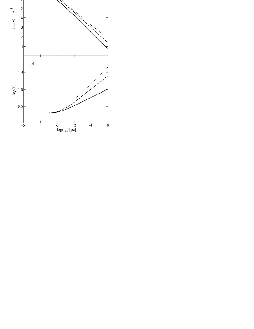
Figure 3: Transversal profile of the number density $n_{\rm e}$ (a) and Lorentz factor $\Gamma$ (b) in logarithmical scale for $\lambda=10^{13}$, jet radius $R_{\rm jet}=1$ pc and three different values of $\sigma$: 5 (solid line), 15 (dashed line), and 30 (dotted line).

4 On the internal structure of jets

As was shown by Beskin & Malyshkin (2000); Beskin & Nokhrina (2009); Lyubarsky (2009), for well-collimated jets the one-dimensional cylindrical MHD approximation (when the problem is reduced to the system of two ordinary differential equations, see above mentioned papers for more detail) allows us to reproduce main results obtained later by two-dimensional numerical simulation (Komissarov et al., 2006; Tchekhovskoy et al., 2009; Porth et al., 2011; McKinney et al., 2012). In particular, both analytical and numerical consideration predict the existence of a dense core in the centre of a jet for low enough ambient pressure $P_{\rm ext}$. Thus, knowing main parameters obtained above we can determine the transverse structure of jets using rather simple 1D analytical approximation. The only parameters we need are the Michel magnetization $\sigma_{\rm M}$ and the transverse dimension of a jet $R_{\rm jet}$ (or, the ambient pressure $P_{\rm ext}$). In particular, transversal profiles of the Lorentz factor $\Gamma$, number density $n_{\rm e}$, and magnetic field $B$ can be well reproduced. In this section we apply this approach to clarify the real structure of relativistic jets.

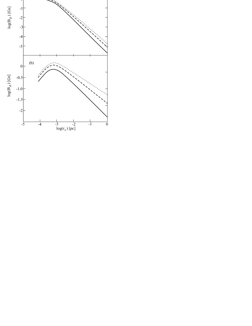
Figure 4: Transversal profile of poloidal (a) and toroidal (b) components of magnetic field in logarithmical scale for the same parameters and line types as in Fig. 3.

In Fig. 3 we present logarithmic plots of Lorentz factor and number density across the jet for $\lambda=10^{13}$, jet radius $R_{\rm jet}=1$ pc and $\sigma=5$, 15, and 30. Fig. 4 shows logarithmic plots of poloidal and toroidal components of magnetic field across the jet with the same parameters as in Fig. 3. As we see, these results point to the existence of more dense central core in the centre of a jet. Indeed, for our parameters the number density in the center of a jet is greater by a factor of a thousand than at the edge. However the Lorentz factor in the central core is small (see Fig. 3b). Thus, these results are in qualitative agreement with previous studies.

Knowing how the Lorentz factor on the edge of jet depends on its radius and making a simple assumption about the form of the jet, we can calculate the dependence of the Lorentz factor on the coordinate along the jet. The result is presented in Fig. 5 for the cases of parabolic $\zeta\propto r_{\perp}^{2}$ and $\zeta\propto r_{\perp}^{3}$ form of the jet. Here $\zeta$ is the distance along the axis. We also assume that the jet has a radius of about 10 pc at the distance 100 pc in both cases, which corresponds to a half-opening angle of the jet $\theta_{\rm jet}\approx 0.1$. According to Fig. 5, particle acceleration in the frame of the AGN host galaxy on the scales 60–100 pc has values about $\dot{\Gamma}/\Gamma=10^{-3}$ per year with very little dependence of this value on the particular form of a jet boundary. This agrees nicely with results of the VLBI acceleration study in AGN jets by Homan et al. (2009, 2015).

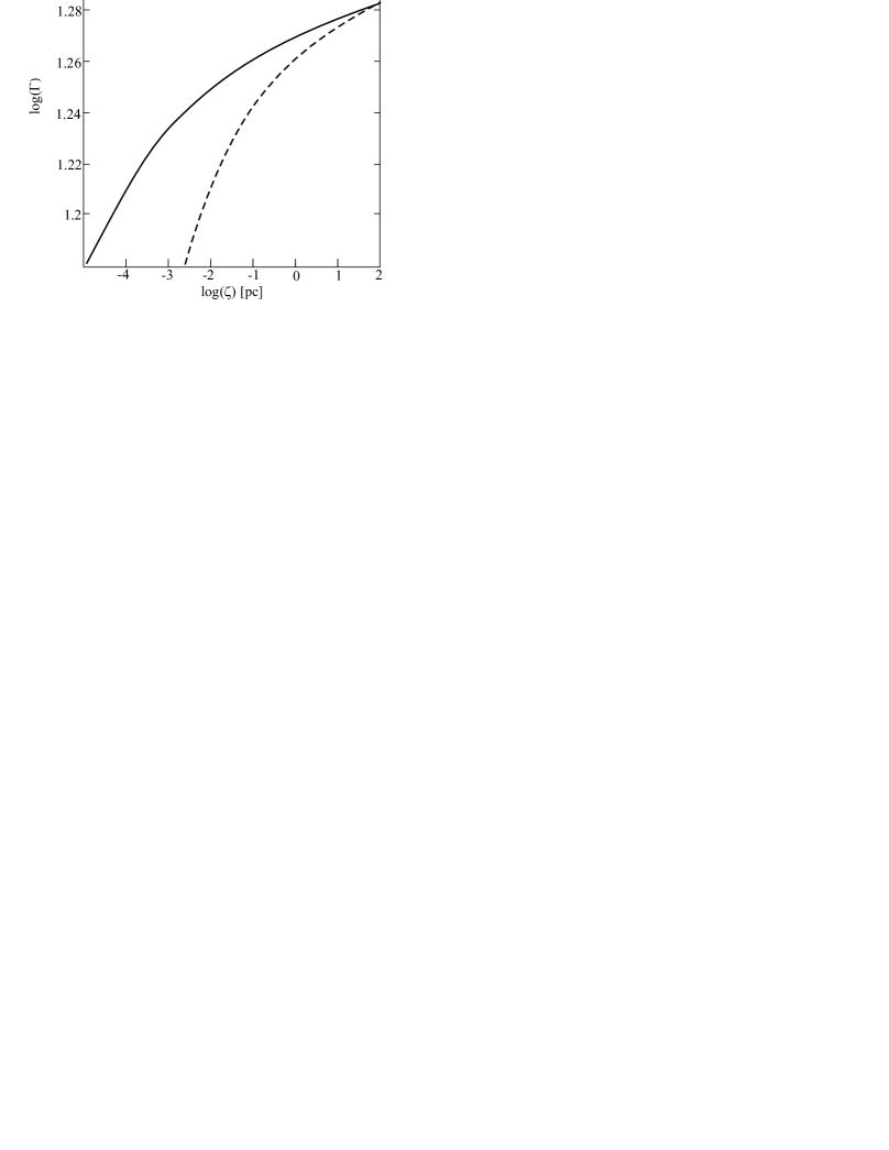
Figure 5: Dependence of Lorentz factor on coordinate along the jet in assumption of parabolic $\zeta\propto r_{\perp}^{3}$ (solid line) and $\zeta\propto r_{\perp}^{2}$ (dashed line) form of the jet.

5 Studying the causal connectivity of the cylindrical jet model

The calculated multiplication parameter $\lambda$ with Michel magnetization $\sigma_{\rm M}$ as well as the observed half-opening angle of a jet $\chi$ allow us to test causal connectivity across a jet for the cylindrical model. Every spacial point of a super-magnetosonic outflow has its own “Mach cone” of causal influence. In case of a uniform flow the cone originating at the given point with its surface formed by the characteristics of a flow is a domain, where any signal from the point is known. For a non-uniform flow the cone becomes some vortex-like shape, depending on the flow property, but sustaining the property of a causal domain for a given point.

In a jet, if the characteristic inlet from any point of a set of boundary points reaches the jet axis, we say that the axis is causally connected with the boundary. On the contrary, if there is a characteristic that does not reach the axis, we have a causally disconnected flow. In the latter case, a question arises about the self-consistency of an MHD solution of the flow, since the inner parts of such a flow do not have any information about the properties of the confining medium. The examples of importance of causal connectivity in a flow and its connection with the effective plasma acceleration has been pointed out by Komissarov et al. (2009) and Tchekhovskoy et al. (2009).

In the case of the cylindrical jet model the question of casuality is even more severe. For a cylindrical model we take into account the force balance across a jet only, so the trans-field equation governing the flow becomes one-dimensional. For every initial condition at the axis its solution gives the flow profile and the position of a boundary, defined so as to contain the whole magnetic flux. Any physical value at the boundary such as, for example, the pressure, may be calculated from this solution. Or, we in fact reverse the problem, and for a given outer pressure at the boundary we find the initial conditions at the jet axis. Thus, we use the dependence of the jet properties at the axis from the conditions at the boundary. In this case, the boundary and the axis must be causally connected. In other words, for a strictly cylindrical flow the conditions at the boundary at the distance $\zeta_{0}$ from the jet origin must be “known” to the point at the axis at the same $\zeta_{0}$.

In the cylindrical model the dynamics of a flow along the jet is achieved by “piling up” the described above cross cuts so as to either make the needed boundary form, or to model the variable outer pressure. In this case the jet boundaries should be constrained by the “Mach cone” following causal connection for the model to be self-consistent.Thus, we come to the following criteria: we may assert that we can neglect the jet-long derivatives in a trans-field equation if any characteristic, outlet from a boundary at $\zeta_{0}$, not only reaches the axis, but does it at $\zeta:\,|\zeta-\zeta_{0}|\ll\zeta_{0}$.

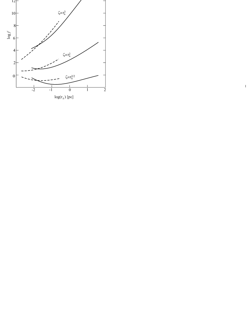
Figure 6: The causality function $f$ for different magnetic surface shapes for $\Gamma>\Gamma_{\mathrm{max}}/2$, i.e. further the equipartition. Solid lines are shown for $\sigma_{\mathrm{M}}=100$ while dotted — for $\sigma_{\mathrm{M}}=10$. The upper curves correspond to $\zeta\propto r_{\perp}^{3}$, the curves in the middle — to $\zeta\propto r_{\perp}^{2}$, and the lower curves — to $\zeta\propto r_{\perp}^{3/2}$.

For an axisymmetric flow the condition of a causal connectivity across the flow may be written (Tchekhovskoy et al., 2009) in the simplest case as

$$\theta_{\rm F}>\theta_{\rm j},$$ (41)

where $\theta_{\rm F}$ is a half-opening angle of a fast Mach cone at the boundary. This condition means that the characteristic from the jet boundary, locally having its half-opening angle $\theta_{\rm F}$ with regard to the local poloidal flow velocity, reaches the axis. For an ultra-relativistic flow, $\theta_{\rm F}$ may be defined as (Tchekhovskoy et al., 2009)

$$\sin^{2}\theta_{\rm F}=\frac{1}{M^{2}_{\rm F}}=\frac{\Gamma_{\rm max}-\Gamma}{\Gamma^{3}}.$$ (42)

In the cylindrical approach, we can check the causal connection across the jet both by applying condition (41), and by tracking the net of characteristics, outlet from the boundary. This can be done for a different jet boundary shapes. Let us introduce the causality function

$$f=\frac{\Gamma_{\rm max}-\Gamma}{\Gamma^{3}}\cdot\frac{1}{\sin^{2}\theta_{\rm j}}.$$ (43)

It follows from (41) and (42) that for $f>1$ causal connectivity holds, and for $f<1$ it does not. If a jet boundary form is given by a function $\zeta=\zeta(r_{\perp})$, where $r_{\perp}$ is an axial radius, the half-opening jet angle is defined by

$$\sin\theta_{\rm j}=\frac{\partial r_{\perp}}{\partial\zeta}\left[1+\left(\frac{\partial r_{\perp}}{\partial\zeta}\right)^{2}\right]^{-1/2}.$$ (44)

Fig. 6 shows the causality function for a paraboloidal flow (see Beskin & Nokhrina, 2009) $\zeta\propto r_{\perp}^{2}$, for a jet with a boundary shaped as $\zeta\propto r_{\perp}^{3}$, and $\zeta\propto r_{\perp}^{3/2}$. For the latter flow shape $f<1$ for every distance. Thus, the first two outflows are causally connected, and the last one may be causally disconnected. Thus, the first two outflows are causally connected, and the last one may be causally disconnected.

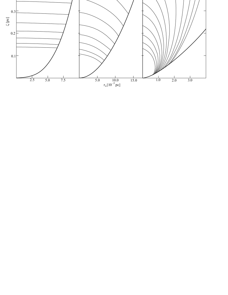
Figure 7: The net of inbound characteristics for a parabolic form of a jet boundary $\zeta\propto r_{\perp}^{3}$ (left panel), $\zeta\propto r_{\perp}^{2}$ (center panel), $\zeta\propto r_{\perp}^{3/2}$ (right panel).

The cylindrical approach allows us to investigate the set of characteristics to check the causality of a flow. Let us discuss the paraboloidal flow first. We can calculate the Mach half-opening angle at each point, starting from the boundary, and so tracking the exact characteristics. This half-opening angle is defined with regard to the flow velocity direction. Although in the cylindrical approach all the velocities have only the $\zeta$-component, we may introduce the $r_{\perp}$-component by taking into account the given form of each magnetic surface. The latter is defined by the function

$$X=\sqrt{r_{\perp}^{2}+\zeta^{2}}-\zeta={\rm const},$$ (45)

and for inner parts of a flow $\Psi=\Psi_{0}X$. Thus, we define the angle $\theta_{\ell}$ of a field-line tangent to a vertical direction as ${\rm tg}\theta_{\ell}=\left|B_{r_{\perp}}\right|/\left|B_{\zeta}\right|=\partial r_{\perp}/\partial\zeta$, and at the given point of a flow we outlet the fast characteristic with regard to thus defined flow direction. We present in Fig. 7 (center panel) the net of characteristics for a paraboloidal flow depicted as described above. The characteristics are calculated starting from the jet boundary towards the axis. They are parameterized by the square of fast magnetosonic Mach number $M_{\mathrm{F}}^{2}$ at the axis at the same $\zeta$, where the characteristic starts. This is done uniformly regarding the Mach number, thus the characteristics are plotted at different distances from each other. It can be seen that all the characteristics for parabolic jet boundary reach the axis at $\zeta$ not much greater than $\zeta_{0}$. The same result holds for a flow $\zeta\propto r_{\perp}^{3}$ either (see Fig. 7, left panel). On the contrary, each characteristic, depicted in Fig. 7 (right panel) for a flow $\zeta\propto r_{\perp}^{3/2}$, reaches the axis at a distance along a flow much greater than the $\zeta$-coordinate of its origin. This suggests that the cylindrical approach is definitely not valid in this case.

6 Discussion

We show that the multiplicity parameter $\lambda$, which is the ratio of number density $n_{\rm e}$ of outflowing plasma to Goldreich-Julian number density $n_{\rm GJ}$, can be obtained from the direct observations of core shift, apparent opening angle and radio power of a jet. The formula (31) uses the following assumptions, taken from the theoretical model: (i) the acceleration process of plasma effectivily stops (saturates) when there is an equipartion regime, i.e. the Poynting flux is equal to the plasma kinetic energy flux; (ii) we assume the certain power-law scalings for magnetic field $B(r)$ and number density $n_{\rm e}(r)$ as a functions of distance $r$ (Lobanov, 1998). These scalings are confirmed by Sokolovsky et al. (2011). We also see that these power-laws are a good approximation from modelling the internal jet structure in section 4.

In contrast with Lobanov (1998) and Hirotani (2005) we do not assume the equipartition regime of radiating particles with magnetic field, but the relation between the particles (radiating and non-radiating) kinetic energy and Poynting flux. We assume that only the small fraction of particles $\sim 1\%$ radiates (Sironi, Spitkovsky & Arons, 2013) and introduce the correlation between particle number density and magnetic field through the flow magnetization $\sigma$. Although for $\sigma\sim 1$ both approaches give effectively the same relation between particle number density and magnetic field, for highly magnetized regime $\sigma\gg 1$ our approach yields the different result. Probing both the equipartion regime $\sigma\sim 1$ and highly magnetized regime $\sigma\gg 1$ at parsec scales we conclude that the latter does not hold.

Using the obtained Michel magnetization parameter $\sigma_{\rm M}$, one can easily explain the observationally derived values $2\Gamma\chi\approx 0.1$ (Clausen-Brown et al., 2013; Zamaninasab et al., 2014), where $\Gamma$ is Lorentz factor of bulk plasma motion and $\chi$ is a jet half-openong angle. Indeed, as was found by Tchekhovskoy et al. (2008); Beskin (2010), $2\Gamma\chi\approx 1$ in the whole domain where $\Gamma\ll\sigma$, independent of the collimation geometry. This implies that $2\Gamma\chi\approx 1$ up to the distance from the origin whence the transverse dimension of a jet $R_{\mathrm{jet}}/R_{\mathrm{L}}=\sigma_{\rm M}$. At larger distances $\Gamma$ remains practically constant, but for a parabolic geometry the opening angle decreases with the distance $\zeta$ as $\zeta^{-1/2}\approx r^{-1/2}$. As a result, one can write down

$$2\Gamma\chi\sim\sqrt{\frac{\sigma_{\rm M}R_{\mathrm{L}}}{R_{\mathrm{jet}}}}\sim 0.1.$$ (46)

This result is in agreement with the criteria of casual connectivity across a jet. Indeed, for an outflow with an equipartition between the Poynting and particle energy flux, we can write down

$$2\Gamma\chi=\frac{1}{\sqrt{f}}<1$$ (47)

for a boundary causally connected with an axis. In Section 5 we have shown that for flows collimated better than a parabola, casuality connectivity across the jet holds further, i.e. for $\Gamma>\Gamma_{\rm max}/2$.

7 Summary

The analysis of the frequency dependence of the observed shift of the core of relativistic AGN jets allows us to determine physical parameters of the jets such as the plasma number density and the magnetic field inside the flow. We have estimated the multiplicity parameter $\lambda$ to be of the order $10^{12}$–$10^{15}$. It is consistent with the Blandford-Znajek model (Blandford & Znajek, 1977) of the electron-positron generation in the magnetosphere of the black hole (see Moscibrodzka et al., 2011, as well). These values are in agreement with the particle number density $n_{\mathrm{e}}$ which was found independently by Lobanov (1998).

As the transverse jet structure depends strongly on the flow regime, whether it is in equipartition or magnetically dominated, it is imporatant to know the relation between the observed and maximum Lorentz factor. The Michel magnetization parameter $\sigma_{\mathrm{M}}$ is equal to the maximum Lorentz factor of plasma bulk motion. Typical derived values of $\sigma_{\mathrm{M}}\lesssim 30$, in agreement with the Lorentz factor estimated from VLBI jet kinematics (e.g., Cohen et al., 2007; Lister et al., 2009a, 2013) and radio variability (Jorstad et al., 2005; Hovatta et al., 2009; Savolainen et al., 2010). This implies that a flow is in the saturation regime. Since for strongly collimated flow the condition of causial connection is fullfilled (see, e.g., Komissarov et al. (2009); Tchekhovskoy et al. (2009)), the internal structure of an outflow can be modelled within the cylindrical approach (Beskin & Malyshkin, 2000; Beskin & Nokhrina, 2009). It has been shown that the results of the modelling, such as Lorentz factor dependence on the jet distance, are in a good agreement with the observations. In particular, the relative growth of Lorentz factor $\dot{\Gamma}/\Gamma$ with the distance along the axis is slow for the jets in saturation regime, having the magnitude $\sim 10^{-3}$ per year. This result may account for the recent masurements of acceleration in AGN jets (Homan et al., 2015).

We plan to address the following points in a separate paper: (i) the role of the inhomogeneity of the magnetic field and particle number density in a core, (ii) the action of the radiation drag force (Li, Begelman & Chiueh, 1992; Beskin, Zakamska, & Sol, 2004; Russo & Thompson, 2013), (iii) the possible influence of mass loading (Komissarov, 1994; Stern & Poutanen, 2006; Derishev et al., 2003) on the jet magnetization and dynamics.

Table 1: Jet parameters and derived multiplication and magnetization parameters.

Source	z	$\beta_{\mathrm{app}}$	$\chi_{\mathrm{app}}$	$S_{0.3}$	$P_{\rm jet}$	Reference	$\Delta r_{\rm core}$	Epoch	$\lambda$	$\sigma$
		($c$)	(∘)	(Jy)	($10^{45}$ erg/s)	for $S_{0.3}$	(mas)	for $\Delta r_{\rm core}$	($10^{13}$)
(1)	(2)	(3)	(4)	(5)	(6)	(7)	(8)	(9)	(10)	(11)
0003$-$066	0.347	8.40	16.3	2.17	1.07	2	0.035	2006-07-07	1.21	9.69
0106$+$013	2.099	24.37	23.6	2.85	10.50	6	0.005	2006-07-07	2.02	23.67
0119$+$115	0.570	18.57	15.6	2.24	1.86	6	0.347	2006-06-15	3.84	4.27
0133$+$476	0.859	15.36	21.7	1.63	2.54	8	0.131	2006-08-09	3.52	5.80
0202$+$149	0.405	15.89	16.4	6.25	2.39	3	0.122	2006-09-06	1.63	10.90
0202$+$319	1.466	10.15	13.4	0.76	2.99	8	0.013	2006-08-09	2.17	11.13
0212$+$735	2.367	6.55	16.4	1.54	5.17	8	0.149	2006-07-07	9.82	4.41
0215$+$015	1.715	25.06	36.7	0.88	3.90	5	0.088	2006-04-28	3.75	7.54
							0.241	2006-12-01	7.97	3.54
0234$+$285	1.206	21.99	19.8	1.45	3.52	5	0.275	2006-09-06	5.29	4.79
0333$+$321	1.259	13.07	8.0	3.68	6.72	7	0.279	2006-07-07	4.10	8.62
0336$-$019	0.852	24.45	26.8	2.49	3.26	6	0.117	2006-08-09	2.66	8.68
0403$-$132	0.571	20.80	16.4	7.62	4.45	2	0.346	2006-05-24	3.66	6.95
0420$-$014	0.916	5.74	22.7	0.87	1.84	3	0.267	2006-10-06	13.49	1.30
0458$-$020	2.286	13.57	23.1	3.54	11.20	3	0.006	2006-11-10	3.20	17.26
0528$+$134	2.070	17.34	16.1	1.02	5.85	2	0.167	2006-10-06	4.81	7.40
0529$+$075	1.254	18.03	56.4	1.75	4.54	2	0.110	2006-08-09	3.83	7.58
0605$-$085	0.870	19.19	14.0	1.43	2.39	3	0.096	2006-11-10	1.66	11.95
0607$-$157	0.323	1.918	35.1	2.31	0.96	3	0.240	2006-09-06	28.46	0.38
0642$+$449	3.396	8.53	23.4	0.70	7.68	8	0.110	2006-10-06	5.27	8.29
0730$+$504	0.720	14.07	14.8	0.71	1.20	8	0.262	2006-05-24	4.27	3.21
0735$+$178	0.450	5.04	21.0	1.81	1.23	8	0.039	2006-04-28	2.56	5.07
0736$+$017	0.189	13.79	17.9	1.79	0.42	3	0.079	2006-06-15	0.82	8.38
0738$+$313	0.631	10.72	10.5	1.26	1.48	3	0.183	2006-09-06	2.85	5.23
0748$+$126	0.889	14.58	16.2	1.45	2.65	2	0.098	2006-08-09	2.41	8.69
0754$+$100	0.266	14.40	13.7	0.74	0.39	2	0.266	2006-04-28	2.06	3.32
0804$+$499	1.436	1.15	35.3	0.60	2.49	8	0.094	2006-10-06	35.88	0.61
0805$-$077	1.837	41.76	18.8	2.60	9.26	2	0.207	2006-05-24	3.12	14.09
0823$+$033	0.505	12.88	13.4	0.63	0.71	5	0.141	2006-06-15	2.12	4.71
0827$+$243	0.942	19.81	14.6	0.71	1.80	2	0.150	2006-05-24	2.52	6.92
0829$+$046	0.174	10.13	18.7	0.67	0.21	2	0.109	2006-07-07	1.28	3.82
0836$+$710	2.218	21.08	12.4	5.06	17.75	2	0.186	2006-09-06	3.81	16.43
0851$+$202	0.306	15.14	28.5	1.11	0.56	3	0.028	2006-04-28	1.08	7.69
0906$+$015	1.026	22.08	17.5	1.54	3.05	3	0.168	2006-10-06	3.04	7.56
0917$+$624	1.453	12.07	15.9	1.27	4.07	8	0.112	2006-08-09	3.95	7.14
0923$+$392	0.695	2.76	10.8	3.28	3.03	5	0.042	2006-07-07	3.23	6.69
0945$+$408	1.249	20.20	14.0	2.94	6.30	2	0.083	2006-06-15	1.80	18.92
1036$+$054	0.473	5.72	6.5	0.75	0.80	2	0.195	2006-05-24	2.77	3.80
1038$+$064	1.265	10.69	6.7	1.59	4.32	2	0.106	2006-10-06	2.02	14.01
1045$-$188	0.595	10.51	8.0	2.79	2.46	2	0.156	2006-09-06	2.01	9.45
1127$-$145	1.184	14.89	16.1	5.63	8.94	6	0.096	2006-08-09	2.73	14.77
1150$+$812	1.250	10.11	15.0	1.39	3.81	8	0.087	2006-06-15	3.31	8.03
1156$+$295	0.725	24.59	16.7	4.33	3.89	8	0.162	2006-09-06	2.15	11.40
1219$+$044	0.966	0.82	13.0	1.14	2.52	4	0.133	2006-05-24	22.11	0.94
1219$+$285	0.103	9.12	13.9	1.77	0.19	3	0.182	2006-02-12	1.11	4.04
							0.142	2007-04-30	0.93	4.87
							0.199	2006-11-10	1.19	3.78
1222$+$216	0.434	26.60	10.8	3.98	1.90	5	0.180	2006-04-28	1.14	14.13
1226$+$023	0.158	14.86	10	63.72	3.25	3	0.020	2006-03-09	0.31	60.77
1253$-$055	0.536	20.58	14.4	16.56	6.31	3	0.048	2006-04-05	0.75	39.84
1308$+$326	0.997	27.48	18.5	1.42	2.79	8	0.143	2006-07-07	2.35	9.33
1334$-$127	0.539	16.33	12.6	1.91	1.71	2	0.237	2006-10-06	2.61	5.98
1413$+$135	0.247	1.78	8.8	2.74	0.81	2	0.230	2006-08-09	6.02	1.64
1458$+$718	0.904	6.61	4.5	19.64	13.30	8	0.081	2006-09-06	1.46	32.22
							0.136	2007-03-01	2.16	21.84
1502$+$106	1.839	17.53	37.9	1.08	4.92	3	0.052	2006-07-07	3.59	8.92
1504$-$166	0.876	3.94	18.4	1.80	2.79	3	0.148	2006-12-01	9.56	2.05
1510$-$089	0.360	28.00	15.2	2.75	1.22	3	0.122	2006-04-28	0.93	13.47
1514$-$241	0.049	6.39	7.8	2.06	0.08	3	0.188	2006-04-28	0.56	5.15

Table 2: continued

Source	z	$\beta_{\mathrm{app}}$	$\chi_{\mathrm{app}}$	$S_{0.3}$	$P_{\rm jet}$	Reference	$\Delta r_{\rm core}$	Epoch	$\lambda$	$\sigma$
		($c$)	(∘)	(Jy)	($10^{45}$ erg/s)	for $S_{0.3}$	(mas)	for $\Delta r_{\rm core}$	($10^{13}$)
(1)	(2)	(3)	(4)	(5)	(6)	(7)	(8)	(9)	(10)	(11)
1538$+$149	0.606	8.74	16.1	2.82	2.36	3	0.032	2006-06-15	1.68	11.09
1546$+$027	0.414	12.08	12.9	0.70	0.61	3	0.010	2006-08-09	0.87	10.32
1606$+$106	1.232	19.09	24.0	2.67	5.30	7	0.057	2006-07-07	2.11	14.84
1611$+$343	1.400	29.15	26.9	4.20	8.44	3	0.057	2006-06-15	1.79	22.54
1633$+$382	1.813	29.22	22.6	2.51	8.28	8	0.119	2006-09-06	3.07	13.50
1637$+$574	0.751	13.59	10.7	1.32	1.88	8	0.117	2006-05-24	1.92	8.94
1638$+$398	1.666	15.85	53.8	0.64	3.11	8	0.007	2006-08-09	4.68	5.36
1641$+$399	0.593	19.27	12.9	9.93	5.13	8	0.211	2006-06-15	2.29	11.99
1655$+$077	0.621	14.77	5.5	2.36	2.33	6	0.080	2006-11-10	0.73	25.39
							0.086	2007-06-01	0.77	24.05
1726$+$455	0.717	2.30	16.5	0.49	0.95	8	0.009	2006-09-06	5.18	2.34
1730$-$130	0.902	27.35	10.4	6.46	6.54	3	0.174	2006-07-07	1.67	19.72
1749$+$096	0.322	7.90	16.8	1.20	0.61	6	0.061	2006-06-15	1.43	6.15
1751$+$288	1.118	3.87	12.1	0.40	1.55	2	0.007	2006-10-06	3.60	4.62
1758$+$388	2.092	2.21	17.9	0.18	1.82	8	0.079	2006-11-10	13.98	1.42
1803$+$784	0.680	10.79	18.4	1.92	2.23	8	0.029	2006-09-06	1.71	10.80
							0.061	2007-05-03	1.98	9.31
1823$+$568	0.664	26.17	6.8	2.63	2.52	8	0.052	2006-07-07	0.42	46.21
1828$+$487	0.692	13.07	7.1	47.78	15.60	3	0.117	2006-08-09	1.39	35.35
1849$+$670	0.657	23.08	16.6	0.86	1.22	8	0.024	2006-05-24	0.88	15.50
1908$-$201	1.119	4.39	23.9	2.70	5.21	2	0.246	2006-03-09	18.03	1.69
1928$+$738	0.302	8.17	9.8	4.81	1.40	8	0.147	2006-04-28	1.72	7.66
1936$-$155	1.657	5.34	35.2	0.67	3.45	2	0.215	2006-07-07	22.92	1.15
2008$-$159	1.180	4.85	9.7	0.73	2.41	2	0.008	2006-11-10	2.65	7.89
2022$-$077	1.388	23.23	19.6	2.63	6.67	2	0.006	2006-04-05	1.51	23.67
2121$+$053	1.941	11.66	34.0	0.63	3.99	2	0.152	2006-06-15	10.29	2.83
2128$-$123	0.501	5.99	5.0	1.47	1.23	3	0.223	2006-10-06	2.52	5.20
2131$-$021	1.284	19.96	18.4	2.66	6.11	6	0.089	2006-08-09	2.39	14.14
2134$+$004	1.932	5.04	15.2	0.99	4.85	6	0.188	2006-07-07	12.35	2.60
2136$+$141	2.427	4.15	32.5	0.94	6.16	6	0.008	2006-09-06	10.28	3.64
2145$+$067	0.999	2.83	23.2	3.76	5.18	3	0.008	2006-10-06	6.97	4.31
2155$-$152	0.672	18.12	17.6	2.41	2.43	3	0.405	2006-12-01	5.34	3.60
2200$+$420	0.069	9.95	26.2	1.82	0.12	8	0.032	2006-04-05	0.47	7.30
2201$+$171	1.076	17.66	13.6	1.00	2.63	2	0.380	2006-05-24	5.64	3.82
2201$+$315	0.295	8.27	12.8	1.82	0.88	3	0.347	2006-10-06	3.90	2.67
							0.192	2007-04-30	2.50	3.80
2209$+$236	1.125	2.29	14.2	0.39	1.51	2	0.038	2006-12-01	6.03	2.73
2216$-$038	0.901	6.73	15.6	2.25	3.57	6	0.011	2006-08-09	2.55	9.57
2223$-$052	1.404	20.34	11.7	13.59	18.00	3	0.199	2006-10-06	3.21	18.33
2227$-$088	1.560	2.00	15.8	1.41	5.14	2	0.186	2006-07-07	22.85	1.40
2230$+$114	1.037	8.62	13.3	8.51	9.25	3	0.278	2006-02-12	7.36	5.45
2243$-$123	0.632	5.24	14.8	1.45	1.71	1	0.161	2006-09-06	5.73	2.79
2251$+$158	0.859	13.77	40.9	12.47	9.39	3	0.124	2006-06-15	8.31	4.72
2345$-$167	0.576	11.47	15.8	2.81	2.21	3	0.167	2006-11-10	3.24	5.54
2351$+$456	1.986	21.56	20.1	2.23	8.54	8	0.196	2006-05-24	5.35	7.99

Notes. Columns are as follows: (1) source name (B1950); (2) redshift $z$ as collected by (Lister et al., 2013); (3) apparent velocity measured by (Lister et al., 2013); (4) apparent opening angle measured by (Pushkarev et al., 2009); (5) flux density at the 92 cm band; (6) derived total jet power; (7) 92 cm flux density reference: 1 — De Breuck et al. (2002), 2 — Douglas et al. (1996), 3 — Ghosh, Gopal-Krishna & Rao (1994), 4 — Gregory & Condon (1991), 5 — Kühr et al. (1979), 6 — Kühr et al. (1981), 7 — Mitchell et al. (1994), 8 — Rengelink et al. (1997); (8) core shift for frequencies $8.1-15.3$ GHz, measured in mas (Sokolovsky et al., 2011; Pushkarev et al., 2012); (9) an epoch of the core shift measurements by Pushkarev et al. (2012) for the year 2006 and by Sokolovsky et al. (2011) for the year 2007; (10) derived multiplicity parameter; (11) derived Michel magnetization parameter.

Appendix A Magnetization parameter

The standart Grad-Shafranov approach for MHD flows uses the following energy integral $E$, conserved at the magnetic flux surface $\Psi$:

$$E(\Psi)=\frac{c\Omega_{\rm F}(\Psi)I}{2\pi}+m\eta(\Psi)c^{2}\Gamma.$$ (48)

Here magnetic field in spherical coordinates $\{r;\,\theta;\,\varphi\}$ is defined by

$$\vec{B}=\frac{\vec{\nabla}\Psi\times\vec{e}_{\varphi}}{2\pi r\sin\theta}-\frac{2I}{cr\sin\theta}\vec{e}_{\varphi},$$ (49)

electric field

$$\vec{E}=-\frac{\Omega_{\rm F}}{2\pi c}\vec{\nabla}\Psi,$$ (50)

$\Omega_{\rm F}$ is a rotational velocity and a function of magnetic flux $\Psi$, $I$ is a current, and

$$\eta(\Psi)=\frac{n_{\rm e,*}|\vec{u}_{\rm p}|}{|\vec{B}_{\rm p}|}=\frac{n_{\rm e}|\vec{v}_{\rm p}|}{|\vec{B}_{\rm p}|}.$$ (51)

Here we assume the flow to be cold, so the particle enthalpy is simply its rest mass. The Poynting vector

$$\vec{S}=\frac{c}{4\pi}\vec{E}\times\vec{B}=\frac{c}{2\pi}\Omega_{\rm F}I\vec{B}_{\rm p}.$$ (52)

The particle kinetic energy flux

$$\vec{K}=\left(\Gamma mc^{2}\right)\left(n_{\rm e}\vec{v}_{p}\right)=\Gamma mc^{2}\eta(\Psi)\vec{B}_{\rm p}.$$ (53)

Thus, we can introduce the magnetization parameter, variable along the flow, as

$$\sigma=\frac{|\vec{S}|}{|\vec{K}|}=\frac{1}{\Gamma}\frac{1}{2\pi c}\frac{\Omega_{\rm F}I}{m\eta}.$$ (54)

On the other hand, there is Michel’s magnetization parameter $\sigma_{\rm M}$, which has a meaning of magnetization at the base of an outflow, is constant, and is defined by

$$\sigma_{\rm M}=\frac{E}{mc^{2}\eta}=\frac{c\Omega_{\rm F}I}{2\pi m\eta c^{2}}+\Gamma=\Gamma\left(\sigma+1\right).$$ (55)

Appendix B Multiplicity parameter

The continuity of relativistic plasma number density flux through two cuts, perpendicular to bulk flow, can be written as

$$\lambda n_{\rm GJ}R_{\rm in}^{2}c=n_{1}\left(r_{1}\chi\right)^{2}c.$$ (56)

Here we assume the flow velocity equal to $c$. Using the expression for the Goldreich-Julian concetration

$$n_{\rm GJ}=\frac{\Omega B}{2\pi ce}$$ (57)

and expression for the full losses due to currents flowing in a magnetosphere

$$P_{\rm jet}=\frac{\left(\Omega B\right)^{2}R_{\rm in}^{4}}{c},$$ (58)

we get

$$n_{1}=\frac{\lambda}{2\pi\left(r_{1}\chi\right)^{2}}\frac{mc^{2}}{e^{2}}\sqrt{\frac{P_{\rm jet}}{P_{\rm A}}}.$$ (59)

References

- Appl & Camenzind (1992) Appl S., Camenzind M., 1992, A&A, 256, 354
- Benford (1981) Benford G., 1981, ApJ, 247, 792
- Beskin (2009) Beskin V.S., 2009, MHD Flows in Compact Astrophysical Objects. Springer, Berlin
- Beskin (2010) Beskin V.S., 2010, Physics-Uspekhi, 53, 1199
- Beskin & Malyshkin (2000) Beskin V.S., Malyshkin L.M., 2000, Astron. Lett., 26, 4
- Beskin & Nokhrina (2009) Beskin V.S., Nokhrina E.E., 2009, MNRAS, 397, 1486
- Beskin, Zakamska, & Sol (2004) Beskin V.S., Zakamska N.L., and Sol H., 2004, MNRAS, 347, 587
- Beskin, Istomin & Pariev (1992) Beskin V.S., Istomin Ya.N., Pariev V.I., 1992, Sov. Astron., 36, 642
- Blandford (1976) Blandford R.D., 1976, MNRAS, 176, 465
- Blandford & Königl (1977) Blandford R.D., Königl A., 1979, ApJ, 232, 34
- Blandford & Znajek (1977) Blandford R.D., Znajek R.L., 1977, MNRAS, 179, 433
- Bisnovatyi-Kogan (2007) Bisnovatyi-Kogan G.S., 2007, Ap & Space Sci, 311, 287
- Bogovalov (1995) Bogovalov S.V., 1995, Astron. Lett., 21, 565
- Cavagnolo et al. (2010) Cavagnolo K.W. et al., 2010, ApJ, 720, 1066
- Clausen-Brown et al. (2013) Clausen-Brown E., Savolainen T., Pushkarev A.B., Kovalev Y.Y., Zensus J.A. 2013, A&A, 558, A144
- Cohen et al. (2007) Cohen M.H. et al, 2007, ApJ, 658, 232
- De Breuck et al. (2002) De Breuck C., Tang Y., de Bruyn A.G., Röttgering H., van Breugel W., 2002, A&A, 394, 59
- Derishev et al. (2003) Derishev E.V., Aharonian F.A., Kocharovsky V.V., Kocharovsky Vl.V., 2003, Phys. Rev. D, 68, 043003
- Douglas et al. (1996) Douglas J.N., Bash F.N., Bozyan F.A, Torrence G.W., Wolfe C., 1996, AJ, 111, 1945
- Ghosh, Gopal-Krishna & Rao (1994) Ghosh T., Gopal-Krishna, Rao A.P., 1994, A&AS, 106, 29
- Goldreich & Julian (1969) Goldreich P., Julian W.H., 1969, ApJ, 157, 869
- Gould (1979) Gould R.J., 1979, A&A, 76, 306
- Gregory & Condon (1991) Gregory P.C., Condon J.J., 1991, ApJS, 75, 1011
- Hardee & Norman (1988) Hardee P.E., Norman M.L., 1988, ApJ, 334, 70
- Heyvaerts & Norman (2003) Heyvaerts J., Norman C., 2003, ApJ, 596, 1240
- Hirotani (2005) Hirotani K., 2005, ApJ, 619, 73
- Hirotani & Okamoto (1998) Hirotani K., Okamoto I., 1998, ApJ, 497, 563
- Homan et al. (2009) Homan D.C. et al., 2009, ApJ, 706, 1253
- Homan et al. (2015) Homan D.C. et al., 2015, ApJ, in press; arXiv:1410.8502
- Hovatta et al. (2009) Hovatta T., Valtaoja E., Tornikoski M., Lähteenmäki A., 2009, A&A, 498, 723
- Istomin & Pariev (1994) Istomin Ya.N., Pariev V.I., 1994, MNRAS, 267, 629
- Jorstad et al. (2005) Jorstad S.G. et al., 2005, Astron. J., 130, 1418
- Komatsu et al. (2009) Komatsu E., Dunkley J., Nolta M.R. et al., 2009, ApJS, 180, 330
- Komissarov (1994) Komissarov S., 1994, MNRAS, 269, 394
- Komissarov et al. (2006) Komissarov S., Barkov M., Vlahakis N., Königl A., 2006, MNRAS, 380, 51
- Komissarov et al. (2009) Komissarov S.S., Vlahakis N., Königl A., Barkov M.V., 2009, MNRAS, 394, 1182
- Kovalev et al. (2008) Kovalev Y.Y., Lobanov A.P., Pushkarev A.B., Zensus J.A., 2008, A&A, 483, 759
- Krolik (1999) Krolik J., 1999, Active galactic nuclei: from the central black hole to the galactic environment. Princeton University Press, Princeton
- Kronberg et al. (2011) Kronberg P.P., Lovelace R.V.E., Lapenta G., Colgate S.A., 2011, ApJ, 741, L15
- Kühr et al. (1979) Kühr H., Nauber U., Pauliny-Toth I.I.K., Witzel A., 1979, MPIfR Preprint, 55, 1
- Kühr et al. (1981) Kühr H., Witzel A., Pauliny-Toth I.I.K., Nauber U., 1981, A&AS, 45, 367
- Li, Begelman & Chiueh (1992) Li Z.-Y., Begelman M., Chiueh T., 1992, ApJ, 384, 567
- Lister et al. (2009a) Lister M.L. et al., 2009a, AJ, 138, 1874
- Lister et al. (2009b) Lister M.L. et al., 2009b, AJ, 137, 3718
- Lister et al. (2013) Lister M. L. et al., 2013, AJ, 146, 120
- Lobanov (1998) Lobanov A.P., 1998, A&A, 330, 79
- Lovelace (1976) Lovelace R.W.E., 1976, Nature, 262, 649
- Lyubarsky (2009) Lyubarsky Yu.E., 2009, ApJ, 308, 1006
- Lyutikov, Pariev & Gabuzda (2005) Lyutikov M., Pariev V.I., Gabuzda D.C., 2005, MNRAS, 360, 869
- Marscher (1983) Marscher A.P., 1983, ApJ, 264, 296
- McKinney et al. (2012) McKinney J.C., Tchekhovskoy A., Blanford R.D., 2012, MNRAS, 423, 2083
- Mestel (1999) Mestel L., 1999, Stellar magnetism. Clarendon Press, Oxford
- Michel (1969) Michel F.C., 1969, ApJ, 158, 727
- Mitchell et al. (1994) Mitchell K.J. et al., 1994, ApJS, 93, 441
- Moscibrodzka et al. (2011) Moscibrodzka M., Gammie C.F., Dolence J.C., Shiokawa H., 2011, ApJ, 735, 9
- Okamoto (2009) Okamoto I., 2009, PASJ, 61, 971
- O’Sullivan & Gabuzda (2009) O’Sullivan S.P., Gabuzda D.C., 2009, MNRAS, 400, 26
- Pariev, Istomin & Beresnyak (2003) Pariev V.I., Istomin Ya.N., Beresnyak A.R., 2003, A&A, 403, 805
- Porth et al. (2011) Porth O., Fendt Ch., Meliani Z., Vaidya B., 2011, ApJ, 737, 42
- Punsly (2001) Punsly B., 2001, Black Hole Gravitohydromagnetics. Springer, Berlin
- Pushkarev et al. (2009) Pushkarev A.B., Kovalev Y.Y., Lister M.L., Savolainen T., 2009, A&A, 507, L33-L36
- Pushkarev et al. (2012) Pushkarev A.B., Hovatta T., Kovalev Y.Y. et al., 2012, A&A, 545, A113
- Rengelink et al. (1997) Rengelink R.B. et al., 1997, A&AS, 124, 259
- Russo & Thompson (2013) Russo M., Thompson Ch., 2013, ApJ, 767, 142
- Savolainen et al. (2010) Savolainen T., Homan D.C., Hovatta T., Kadler M., Kovalev Y.Y., Lister M.L., Ros E., Zensus J.A., 2010, A&A, 512, A24
- Sironi, Spitkovsky & Arons (2013) Sironi L., Spitkovsky A., Arons J., 2013, ApJ, 771, 54
- Sokolovsky et al. (2011) Sokolovsky K.V. et al., 2011, A&A, 532, A38
- Stern & Poutanen (2006) Stern B.E. and Poutanen J., 2006, MNRAS, 372, 1217
- Tchekhovskoy et al. (2008) Tchekhovskoy A., McKinney J., Narayan R., 2008, MNRAS, 388, 551
- Tchekhovskoy et al. (2009) Tchekhovskoy A., McKinney J., Narayan R., 2009, ApJ, 699, 1789
- Verkhodanov et al. (1997) Verkhodanov O.V., Trushkin S.A., Andernach H., Cherenkov V.N., 1997, ASP Conf. Ser. 125, Astronomical Data Analysis Software and Systems VI, ed. G. Hunt & H. Payne (San Fransisco, CA: ASP), 322
- Zamaninasab et al. (2014) Zamaninasab M., Clausen-Brown E., Savolainen T., Tchekhovskoy A., 2014, Nature, 510, 126
- Zdziarski et al. (2014) Zdziarski A.A., Sikora M., Pjanka P., Tchekhovskoy A., 2014, MNRAS, submitted; arXiv:1410.7310