Abstract

We study the modelling and valuation of surrender and other behavioural options in life insurance and pension. We place ourselves in between the two extremes of completely arbitrary intervention and optimal intervention by the policyholder. We present a method that is based on differential equations and that can be used to approximate contract values when policyholders exhibit optimal behaviour. This presentation includes a specification of sufficient conditions for both consistency of the model and convergence of the contract values. When not going to the limit in the approximation we obtain a technique for balancing off arbitrary and optimal behaviour in a simple, intuitive way. This leads to our suggestions for intervention models where one single parameter reflects the extent of rationality among policyholders. In a series of numerical examples we illustrate the impact of the rationality parameter on the contract values.
Keywords: Behavioural option, Ordinary differential equation, Penalty method, Optimal stopping, Solvency II

1 Introduction

Modern solvency and accounting rules (Solvency II and IFRS) require that expected policyholder behaviour is taken into account. This includes e.g. expected surrender and expected transcription into free policy (paid-up policy). The expectation is supposed to take into account both the economic conditions under which the behaviour takes place as well as the extent to which intervention is to the benefit of the policyholder. The economic conditions and how beneficial it is for the policyholder to intervene may change over time. Therefore, one should properly speak of dynamic behaviour models when formalizing these effects in the actuarial valuation formulas. Changing economic conditions could e.g. be a changing level of interest rates, and one idea would be to let the intensity or probability of intervention depend on the current (possibly stochastic) level of interest rates. How beneficial an action is can be formalized by the gain from intervention. Determining the gain may be a delicate issue since both intervening and not intervening opens up for new intervention options in the future that also have to be taken into account. E.g., not to surrender typically opens up for surrendering later, and transcription into free policy changes the effect of the surrender option. This challenge calls for a recursive solution such that the gain is always measuring correctly the tendencies of intervening in the future. We disregard the economic condition by assuming deterministic interest rates and focus on the latter idea of a recursive formula to deal with the benefit of intervention. One motivation for this focus is that, perhaps, the external economic conditions are supposed to approximate to the internal benefit.

There exists a range of approaches to modelling of behavioural risk. One extreme is to say that intervention occurs in a completely arbitrary way, like insurance risk. We hereby mean that we model the behaviour as independent of everything else in our model than the state of the policyholder and the time measured through calendar time, the policyholder’s age, time since initiation, or time to (deterministic) retirement. Specifically, the behaviour depends on neither the contract the policyholder holds nor the interest rate. With this approach it is tractable to study various aspects beyond just adding surrender to a survival model. Buchardt et al. [3] studied the formalistic interaction between semi-Markov modelling of insurance risk and behavioural risk, including duration dependence of mortality and payments in the disability state and recognizing duration dependence of free policy payments. A simpler exposition is found in Buchardt and Møller [2]. Henriksen et al. [9] also combine surrender and free policy options and study the impact on reserving from different simplifying assumptions about the dependence between insurance risk and behaviour risk.

Another extreme is to say that intervention occurs in a completely rational, optimal way. We hereby mean that the policyholder, who is assumed to have the same information as the insurance company has, intervenes according to a strategy that maximizes the value of the insurance contract. This approach was taken in Steffensen [13], who derived general variational inequalities that characterize the reserve in case of a multi-state Markov model for insurance risk and a multi-state model for behavioural risk. In the surrender case, this is known as American option pricing of surrender risk. Other early references based on this approach to surrender risk are Grosen and Jørgensen [8] and Bacinello [1].

In between these extremes exist all different kinds of models where intervention is modelled by an intensity, but where the intensity not only depends on time but also some stochastic factors. The dependence on the interest rate appears obvious and is thoroughly examined by De Giovanni [7], who calculate reserves by solving partial differential equations numerically. There exists a large amount of literature examining relevant explanatory variables but since these studies appear somewhat marginal to our approach we refer to Eling and Kiesenbauer [4] and references therein for a comprehensive literature overview.

Rather than letting the intensity depend on external factors, one could let the intensity depend on internal factors relevant to the specific policy. That could e.g. be to take the difference between the surrender value and (some notion of the) reserve as a measure of how beneficial an intervention is. If the reserve compared with the surrender value does not take future intervention options into account, the calculation can be split up in two standard exercises: First, calculate the reserve without intervention and then plug this reserve into the intensity for a calculation including surrender. If the reserve compared with the surrender value does take future intervention into account, the (usually) linear Thiele differential equation characterizing the reserve becomes in general a non-linear differential equation. The non-linear term comes from the risk premium with respect to the surrender event that contains a non-linear function of the reserve itself. The rationale for this paper is to take a thorough look at this non-linear differential equation in order to motivate it, interpret it, generalize it, and solve it numerically. Last but not least, we present a probabilistic proof of and clarify sufficient conditions for a convergence result that may seem intuitively clear: If the tendency to intervene tends to zero whenever the gain from intervention is negative and tends to infinity whenever the gain from intervention is positive, we reach in the limit at the reserve based on completely rational behaviour. We establish sufficient convergence of intensities to reach such a conclusion. Thus, our approach to intervention option pricing has two purposes: First, it represents in itself a relevant approach in between the two extremes that, certainly, takes into account the extent to which intervention is to the benefit of the policyholder. Second, for simple parametric forms of the intensity, our calculation approximates the largest possible liability. As such it can be used as a worst-case or stress calculation with respect to surrender risk.

The idea of approximating the maximum value by a series of solutions to differential equation has been known as the penalty method. In computational finance it has been used as an approximation method for American option pricing. In Forsyth and Vetzal [5] the penalty method is compared with alternative techniques for pricing of the American put option. In Gad and Pedersen [6] the modelling of non-rational option holder behaviour is studied in a way similar to what is done here. The contribution of the present paper is three-fold: First, we introduce, to the knowledge of the authors, for the first time the penalty method in intervention option pricing in insurance. Second, we prove sufficient conditions for the convergence to hold. Third, we do not only think of the intensity model as a means of approximating the largest value, but as a highly relevant approach to general intervention option pricing, useful in accounting and solvency. The approach balances arbitrariness and benefit in a simple form, and in some examples we catch the notion of rationality in one single parameter.

2 Standard Setup

Consider a model with a policyholder who is either alive (active) or dead. We assume the state of the policyholder is governed by a state process with a deterministic, continuous death intensity, $\mu(t)$, see Figure 1. Let $I$ be the process indicating whether the policyholder is alive, and let $N$ be the process counting the numbers of deaths of the policyholder.

Figure 1: Standard survival model.

The policyholder is assumed to have the following simple contract. She pays a deterministic premium with continuous intensity $\pi(t)$ until a terminal time, $n$, as long as she is alive. If she is alive at time $n$ she receives a deterministic pension sum $b_{a}(n)$, and if she dies before then upon death she gets a deterministic death sum, $b_{ad}(t)$. Thus, the accumulated payments in the time interval $[0,t]$ is given by the following process of accumulated payments:

$$B(t)=B(0)-\int_{0}^{t}\pi(u)I(u)du+\int_{0}^{t}b_{ad}(u)dN(u)+I(n)b_{a}(n)1_{(t\geq n)},$$

for $t\in[0,n]$. We assume that the market offers a deterministic, continuous interest rate, $r(t)$. We introduce the reserve corresponding to the policyholder being active as the conditional expected present value of future payments,

$$V(t)={\mathbb{E}}\left[\left.\int_{t}^{n}e^{-\int_{t}^{u}r(\tau)d\tau}dB(u)\right|I(t)=1\right].$$

We then know, e.g. from [11], that the reserve, $V$, is continuously differentiable on $[0,n)$ and that it is the solution to Thiele’s differential equation,

$$V^{\prime}(t)=r(t)V(t)+\pi(t)-\mu(t)(b^{ad}(t)-V(t)),$$ (1)

with $V(n-)=b_{a}(n)$.

We now add to our model the possibility that the policyholder surrenders. That is, we add the possibility that the policyholder terminates her contract and instead receives a deterministic, continuous surrender value, $G(t)$. This can, e.g., be added to the model by assuming that the policyholder at any time surrenders with some deterministic, continuous intensity, $\nu(t)$, see Figure 2. We use the term active for when the policy is in force.

Figure 2: Standard surrender model.

Mathematically, the state of surrender is in this model not different from the state of death, except that the associated payments are different. The reserve, $V_{\nu}$, is continuously differentiable and solves the following Thiele’s differential equation, see e.g. [11],

$$V_{\nu}^{\prime}(t)=r(t)V_{\nu}(t)+\pi(t)-\mu(t)\left(b^{ad}(t)-V_{\nu}(t)\right)-\nu(t)\left(G(t)-V_{\nu}(t)\right),$$ (2)

with $V_{\nu}(n-)=b_{a}(n)$.

For $V_{v}$ to be continuously differentiable we need, in general, that $\nu$ is continuous as assumed above. However, what is really needed is that $\nu(t)\left(G(t)-V_{\nu}(t)\right)$ is continuous and this can be obtained even when $\nu$ is discontinuous and properly defined at the point where $G(t)=V_{\nu}(t)$.

The surrender value $G$ can be anything exogenously given. In practice it is, typically, a technical value of the same payment stream based on technical assumptions on interest rates and intensities that we denote by $\left(r^{\ast},\mu^{\ast}\right)$. In that case, the surrender value is the technical reserve $V^{\ast}$ that solves (1) with $\left(r,\mu\right)$ replaced by $\left(r^{\ast},\mu^{\ast}\right)$.

3 Reserve Dependent Surrender

The forthcoming Solvency II regulations requires that the traditional modelling of surrender is revisited. In Article 79 of the Solvency II Directive it is stated that ”Any assumptions made by insurance and reinsurance undertakings with respect to the likelihood that policyholders will exercise contractual options, including lapses and surrender, shall be realistic and based on current and credible information. The assumptions shall take account, either explicitly or implicitly, of the impact that future changes in financial and non-financial conditions may have on the exercise of those options”. Thus, we need to investigate and model what influences the policyholders choice to surrender and we need to be able to calculate the reserves in the more advanced models. In the present section we suggest a way to do this, and discuss our method.

In a more realistic model of surrender we want to be able to express both that surrender is likely influenced by how profitable it is, but also that it is still random. On one hand, we wish surrender to be influenced by how profitable it is, because surrender is a decision the policyholder makes. On the other hand we also have multiple reasons for surrender being random. Randomness is natural because the policyholder most likely lacks information to decide what is profitable. Even if she had all the information that the pension fund has and were able to use it, then her preferences may differ seemingly randomly from the model set up by the pension fund because of the policyholders personal preference and economical situation. She might shift her job and get an offer from a new pension fund or she might need cash for a divorce.

We can obtain randomness in our model by keeping the surrender modelled by an intensity. Further, we model that the policyholders decision depends on how profitable it is by letting the surrender intensity depend on how profitable it is for the policyholder to surrender. If she surrenders at time $t$ she gains $G(t)$, but she loses the rest of the contract including her right to exercise later. Hence, she loses $V_{\nu}(t)$. Therefore, we denote by $G(t)-V_{\nu}(t)$ her profit from surrendering at time $t$. We would like the surrender intensity to be non-negative and increasing in this profit. At first glance this modelling seems to have a problem that the definition of the surrender intensity is circular. However, Theorem 3.1 below gives sufficient conditions for this circular definition not to be a problem.

Theorem 3.1

For some given non-negative function, $h$, consider the following differential equation in the function $U$:

$$U^{\prime}(t)=r(t)U(t)+\pi(t)-\mu(t)(b_{ad}(t)-U(t))-h(t,U(t))(G(t)-U(t)),$$ (3)

with $U(n-)=\Delta B(n)$. Suppose (3) has a unique solution, $U$, and define a surrender intensity by $\nu(t)\equiv h(t,U(t))$. Then $U$ is the reserve when the policyholder chooses to surrender at time $t$ with intensity $\nu(t)$.

Proof: The possible problem in this model is the circular definition of the surrender intensity. However, the existence and uniqueness of the solution to both (2) and (3) ensures that this does not become a problem.

The process $\nu$ defined by $\nu(t)\equiv h(t,U(t))$ is uniquely determined from (3) and the reserve is then uniquely determined from (2). It follows from the definition of $U$ that $U$ solves (2), and then from the uniqueness of the solution to (2) it follows that the reserve is given by $U$.

Once we have decided on a policyholder with a specific policy and a function $h$, and thereby also $\nu$, then for this single policyholder, our model does not differ from a model with a deterministic time dependent surrender intensity as what we had in the classical model of (2). However, when we use the model for pricing a portfolio of insurance contracts for a group of policyholders, then the model assigns different surrender intensities to each policyholder. Thereby, the reserves in general become higher than if we had used a constant surrender intensity or a specific time dependent surrender intensity for the whole portfolio.

The relation between the surrender intensity and the profitability may be chosen in many different ways. Two examples we investigate are:

$$\nu(t)=h(t,V_{\nu}(t))=\psi\exp\{\theta(G(t)-V_{\nu}(t))\},$$ (4)

$$\nu(t)=h(t,V_{\nu}(t))=\theta 1_{(G(t)-V_{\nu}(t)>0)},$$ (5)

where $\psi$, $\theta>0$ are constants. For equation (4), $\psi$ tells about the overall tendency to surrender, whereas $\theta$ tells about how profitability creates deviations from this tendency. For equation (5), $\theta$ controls both. In both cases we speak of $\theta$ as the rationality parameter. Other intensity functions can be chosen and one should choose a functional form which matches with data. The only mathematical requirement is that the function $h$ has to make it possible to use Theorem 3.1.

One immediate drawback of our model is that we most often do not have an explicit solution for the differential equation (3). This implies that we do not have an explicit expression for the reserve. However, we do have algorithms available for numerical solutions to ordinary differential equations.

4 Reserve Dependent Policyholder Behaviour

The idea of modelling behaviour by profit dependent intensities may be used for other applications as well. Within life insurance the policyholder’s choice to convert into free policy (paid-up policy) has some resemblance with the surrender choice. Thereby we may find it reasonable to expand our model with the possibility of conversion into free policy in the same way as we added surrender. Figure 3 displays a simple model where $\nu_{af}$ denotes the intensity of conversion into free policy, $\nu_{as}$ denotes the intensity of surrender when active and $\nu_{fs}$ denotes the intensity of surrender after converted into free policy. Here the term active is used when the policyholder is paying premiums.

Figure 3: Free policy and surrender model.

If all transition intensities are known explicitly, this model is studied in [9]. When a policyholder converts into free policy the payments are reduced depending of the time of conversion. Let $b_{fd}(t,u)$ denote the death sum at time $t$ if converted into free policy at time $u$, let $b_{f}(n,u)$ denote the terminal payment at time $n$ if converted into free policy at time $u$, and let $G_{f}(t,u)$ denote the surrender value at time $t$ when converted into free policy at time $u$. For the reserves we let $V_{a}(t)$ denote the reserve at time $t$ if the policyholder is active, and let $V_{f}(t,u)$ denote the reserve at time $t$ if the policyholder is in the free policy state and converted to free policy at time $u$. Now, we assume that the intensities are reserve dependent and given in the form

$$\nu_{as}(t) = h_{as}(t,V_{a}(t)),$$

$$\nu_{af}(t) = h_{af}(t,V_{a}(t)),$$

$$\nu_{fs}(t,u) = h_{fs}(t,u,V_{f}(t,u)).$$

Then the reserves are given from the following differential equations:

$$\frac{\mathrm{d}}{\mathrm{d}t}V_{a}(t) = r(t)V_{a}(t)+\pi(t)-\mu(t)(b_{ad}(t)-V_{a}(t))$$

$$-h_{as}(t,V_{a}(t))(G(t)-V_{a}(t))-h_{af}(t,V_{a}(t))(V_{f}(t,t)-V_{a}(t)),$$

$$V_{a}(n-) = b_{a}(n),$$

$$\frac{\partial}{\partial t}V_{f}(t,u) = r(t)V_{f}(t,u)-\mu(t)(b_{fd}^{*}(t,u)-V_{f}(t,u))$$

$$-h_{fs}(t,u,V_{f}(t,u))(G^{f}(t,u)-V_{f}(t,u)),$$

$$V_{f}(n-,u) = b_{f}(n,u).$$

The only requirement is that the system of differential equations has a unique solution. However, the differential equations from above are heavy to work with, as we need to solve a new differential equation for each value of $V_{f}(t,t)$. When modelling the free policy option, this problem is usually overcome by introducing a scaling function, $f$, that describes the reduction of payments as a result of the conversion to free policy. Thus, $b_{fd}(t,u)=f(u)b_{ad}(t)$, $b_{f}(n,u)=f(u)b_{a}(n)$ and $G_{f}(t,u)=f(u)G_{f}(t)$. Assume the transition intensity $\nu_{fs}$ does not depend on the time of transition to free policy. Then the prospective reserve, $V_{f}^{*}(t)$, from the free policy state based on the payments $G_{f}(t)$, $b_{ad}(t)$ and $b_{a}(n)$ does not depend on this transition time either, and we get $V_{f}(t,u)=f(u)V_{f}^{*}(t)$ with

$$\frac{\mathrm{d}}{\mathrm{d}t}V_{f}^{*}(t) = r(t)V_{f}^{*}(t)-\mu(t)(b_{ad}(t)-V_{f}^{*}(t))$$

$$-\nu_{fs}(t)(G^{f}(t)-V_{f}^{*}(t)),$$

$$V_{f}^{*}(n-) = b_{a}(n).$$

This makes $V_{f}(t,u)$ a lot easier to calculate. For more on the determination of the reference payments and scaling function, see [9]. Note however that if $\nu_{fs}$ cannot depend on the time of transition to free policy, $u$, then it cannot depend on $G_{f}(t,u)-V_{f}(t,u)$ either and this is a large disadvantage.

To get profit dependent choices we may use

$$\nu_{as}(t) = h_{as}(t,V_{a}(t))=\psi_{as}e^{\theta_{as}(G(t)-V_{a}(t))},$$

$$\nu_{af}(t) = h_{af}(t,V_{a}(t))=\psi_{af}e^{\theta_{ap}(V_{f}(t,t)-V_{a}(t))},$$

$$\nu_{fs}(t,u) = h_{fs}(t,u,V_{f}(t,u))=\psi_{fs}e^{\theta_{fs}(G_{f}(t,u)-V_{f}(t,u))}.$$

5 Approximation of the Worst Case Reserve

In the two previous sections we discussed our model with reserve dependent surrender and we found it being a reasonable model for predicting the dynamics of surrender. However, in the following section we discuss how the model may also be used for determining worst case reserves when the true dynamics of the surrender intensity is not known. This is because our model is a version of what in the literature is known as the penalty method, and a large rationality parameter gives us the worst case reserve.

Typically the technical reserve is paid out upon surrender (potentially minus expenses). In that case, if we take maximum of the technical reserve and the market reserve calculated under the assumption of no surrender, then we get a worst case reserve of either surrendering immediately or never surrender. However, a surrender strategy somewhere in between the two extremes may result in a higher market reserve. For determining the worst case reserve we consider all possible surrender strategies. To do this we construct a more general model. We assume that the transition from active to surrender is governed by a randomized stopping time, $\tau$, with respect to the state of the policyholder, with randomized stopping times being defined as in [12]. That is, the time of surrender may depend on everything but the future time of death and the future interest rate. If the policyholder never surrenders her contract we let $\tau=n$. The model is illustrated in Figure 4. The class of admissible surrender strategies at time $t$ are the variables in $[t,n]$ that are randomized stopping times with respect to the filtration generated from $I$. We denote this class by $\mathcal{T}_{t}$.

Figure 4: Optimal surrender model.

We hereby disregard the possibility that the policyholder has more information about her future time of death than the insurance company has. We do this despite that such knowledge could influence the policyholders decisions.

Let $V_{\tau}$ denote the prospective reserve if the policyholder surrenders according to the randomized stopping time $\tau$. Assume $G(n)=0$, assume $G(n-)\leq V(n-)$ and assume $G$ continuous on $[0,n)$. Then from [11] it follows that $V_{\tau}$ is given by:

$$V_{\tau}(t) = {\mathbb{E}}\left[\left.\int_{t}^{\tau}e^{-\int_{t}^{u}r(x)dx}dB(u)+e^{-\int_{t}^{\tau}r(x)dx}G(\tau)I(\tau)\right|I(t)=1\right]$$

$$= V(t)+{\mathbb{E}}\left[\left.e^{-\int_{t}^{\tau}r(x)dx}G(\tau)I(\tau)-\int_{\tau}^{n}e^{-\int_{t}^{u}r(x)dx}dB(u)\right|I(t)=1\right]$$

$$= V(t)+{\mathbb{E}}\left[\left.e^{-\int_{t}^{\tau}r(x)dx}I(\tau)G(\tau)\right|I(t)=1\right]$$

$$-{\mathbb{E}}\left[\left.e^{-\int_{t}^{\tau}r(x)dx}I(\tau){\mathbb{E}}\left[\left.\int_{\tau}^{n}e^{-\int_{\tau}^{u}r(x)dx}dB(u)\right|\tau,I(\tau)=1\right]\right|I(t)=1\right]$$

$$= V(t)+{\mathbb{E}}\left[\left.e^{-\int_{t}^{\tau}r(x)dx}I(\tau)\left(G(\tau)-V(\tau)\right)\right|I(t)=1\right].$$

Consider the worst case scenario for the pension fund, where the policy holder chooses the surrender strategy as the stopping time, $\tau$, that maximizes $V_{\tau}$. This is an optimal stopping problem. Any classical stopping time from the filtration generated by $I$ must fulfil $\tau I(\tau)=t_{0}I(t_{0})$ for some deterministic $t_{0}\in[t,\infty]$. The reserve is then given by:

$$V_{\tau}(t) = V(t)+{\mathbb{E}}\left[\left.e^{-\int_{t}^{\tau}r(x)dx}I(\tau)\left(G(\tau)-V(\tau)\right)\right|I(t)=1\right]$$

$$= V(t)+e^{-\int_{t}^{t_{0}}r(x)+\mu(x)dx}\left(G(t_{0})-V(t_{0})\right).$$

Thus, for the classical optimal stopping problem, without randomization allowed, it is optimal to choose $t_{0}$ as any time from the set:

$$A_{t}\equiv\arg\max_{u\in[t,n]}\left(e^{-\int_{t}^{u}r(x)+\mu(x)dx}(G(u)-V(u))\right).$$

As the inner part is continuous in $u$ on $[0,n)$ and as $G(n-)-V(n-)<G(n)-V(n)$, then $A_{t}$ must have a largest element. Denote this element by $u^{\ast}$, i.e. let $u^{\ast}(t)\equiv\max A_{t}$, such that $u^{\ast}(t)$ is the latest optimal time to surrender. Let $\tau^{\ast}=u^{\ast}(t)I(u^{\ast}(t))+n(1-I(u^{\ast}(t)))$. We define the worst case reserve, $W$, by:

$$W(t)=\sup_{\tau\in\mathcal{T}_{t}}V_{\tau}(t)=V_{\tau^{\ast}}(t).$$

By a proof similar to the one of the verification theorem of Chapter 9 of [10] it may be seen that $\tau^{\ast}$ is optimal even if we allow randomized surrender strategies.

Now, assume a family of functions, $h_{\theta}$, is implied. Let $\tau_{\theta}$ denote the surrender strategy of surrendering at time $u$ with intensity $\nu_{\theta}(u)=h_{\theta}(G(u)-V_{\nu_{\theta}}(u))$ and let $V_{\theta}=V_{\nu_{\theta}}$ with $V_{\nu_{\theta}}$ as defined in Sect.  3. Let

$$\bar{h}_{\theta}(x)\equiv\sup_{y\leq x}h_{\theta}(y),$$

and

$$\underline{h}_{\theta}(x)\equiv\inf_{y\geq x}h_{\theta}(y).$$

Now, the following holds:

Theorem 5.1

Suppose that for each $\theta\geq 0$ we have that $h_{\theta}$ is defined in a way such that we may use Theorem 3.1 and suppose that the surrender value $G$ is continuous on $[0,n)$ with $G(n-)\leq V(n-)$ and $G(n)=0$. Also assume for $x<0$:

$$\bar{h}_{\theta}(x)\rightarrow 0,\ \ \ \theta\rightarrow\infty,$$ (6)

and for $x>0$:

$$\underline{h}_{\theta}(x)\rightarrow\infty,\ \ \ \theta\rightarrow\infty.$$ (7)

Then, for every $t\in[0,n]$:

$$V_{\theta}(t)\rightarrow W(t),\ \ \ \ \ \theta\rightarrow\infty.$$

For a proof, see the appendix.

Remark 5.1

Some of the details in the proof has been omitted, but a fully detailed proof following the same reasoning for a closely related result for an American Put option may be found in [6]. The fact that the penalty method provides convergence and the rate of convergence is not new. However, we find the proof of our article and of [6] interesting. This is because they visualize how the error terms may be thought of as probabilities of economically bad choices of the policyholder times the loss the policyholder faces from her bad choices.

6 Numerical Examples

In this section we show four examples of how various surrender models impact the development of the reserves in four different interest rate situations. In each example we consider a contract with a constant premium intensity of $\pi=7,000$, a death sum of $b^{ad}=1,000,000$ and a pension sum of $2,000,000$ . All values measured in DKK. These numbers are chosen as they have a realistic level for a Danish pension policy. For fairly realistic numbers in EUR divide by ten. The policyholder is assumed to be 35 years old at time 0 and the time of retirement is at age 65. Time is measured in years and her death intensity is assumed to be given by:

$$\mu(t)=0.0005+10^{5.728-10+0.038*(t+35)}.$$

This is the death intensity from the Danish life table G82 for females. If the policyholder surrenders her contract, she receives a surrender value given by the technical reserve. The technical reserve is based on the same payments as the contract, and on a technical interest rate intensity of $\hat{r}=0.05$. Interest rates are chosen high to better visualize the impact of the choice of surrender intensity. We assume no extra expenses at surrender. Thus, the surrender value is given from the differential equation:

$$G^{\prime}(t)=\hat{r}G(t)+\pi-\mu(t)(b^{ad}-G(t)),$$ (8)

with $G(n-)=2,000,000$. We consider the following five surrender models:

$$\begin{array}[]{llcl}\textrm{Model a}:&\nu^{a}(t)&=&0.05\cdot\exp\{0.000003(G(t)-V_{\theta,\psi}(t))\}\\ \textrm{Model b}:&\nu^{b}(t)&=&0.05\cdot 1_{(G(t)-V_{\theta}(t))}\\ \textrm{Model c}:&\nu^{c}(t)&=&0.05\\ \textrm{Model d}:&\nu^{d}(t)&=&0\\ \textrm{Model e}:&\nu^{e}(t)&=&5\cdot 1_{(G(t)-V_{\theta}(t))}.\end{array}$$

The first three models are based on a surrender intensity of around 5%. The last model is a model with a rationality parameter $\theta=5$, which has been found to be high enough for us to approximate the worst case reserve. Additionally, we consider four different developments of the interest rate, $r$, used for pricing market reserves. For the two first interest rate situations we compare the surrender value and the reserves for the five different surrender models. For the two last interest rate situations we compare the surrender value and the reserves for surrender Model d and Model e.

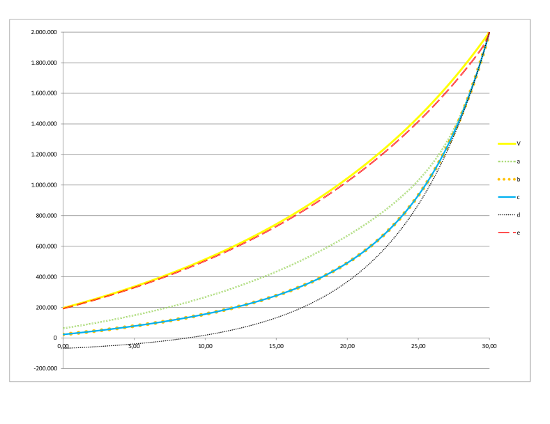
Figure 5: Example 1. The technical interest rate is $\hat{r}=0.05$. The market interest rate is $r=0.12$. Immediate surrender is always optimal.

Example 1: Market interest rate is above technical interest rate

Assume $r=0.12$. The reserve developments are displayed in Figure 5. In this situation it is at all time points optimal for the policyholder to surrender. The worst case reserve corresponds to the surrender value. The lowest reserve is the market reserve based on no surrender, Model d. Models with a chance of surrender has reserves in between. Since there is no risk of surrendering too early, then Model b and the traditional Model c do not differ. For Model a we get a slightly higher reserve than the one for Model b and Model c, because the basic intensity $0.05$ is slightly increased at all time points by the exponential factor in the intensity.

Example 2: Market interest rate is below technical interest rate

Assume $r=0.02$. The reserve developments are displayed in Figure 6. In this situation it is never optimal for the policyholder to surrender. The worst case reserve corresponds to the market reserve with no surrender. In Model b and Model e the policyholder does not make the mistake of surrendering if it is not profitable, and thus, this has an equally high reserve. The surrender value is the lowest value and the reserves of Model a and the traditional Model c are in between. Model a has a higher reserve than Model c, because the basic intensity $0.05$ is slightly increased at all time points by the exponential factor in the intensity.

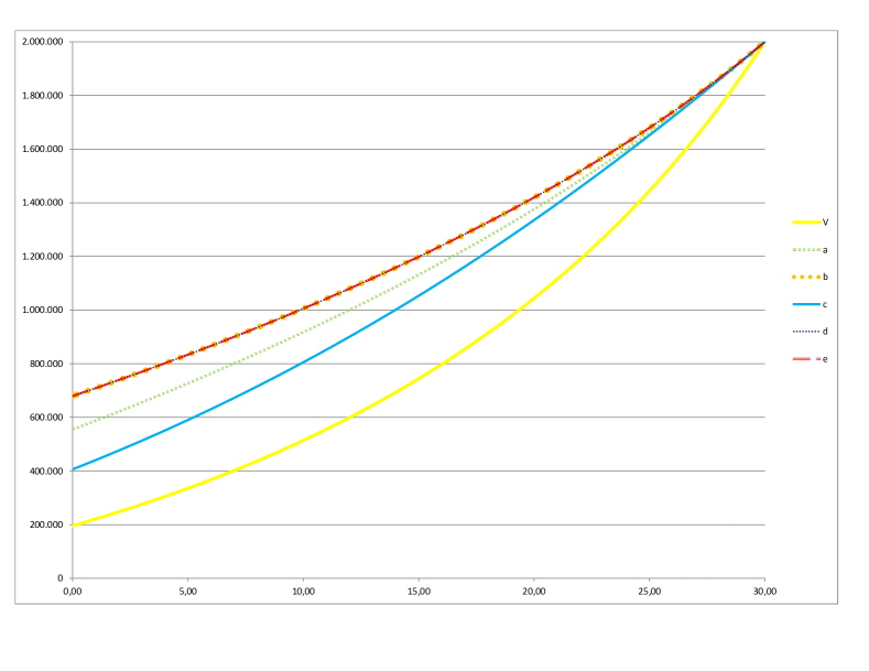
Figure 6: Example 2. The technical interest rate is $\hat{r}=0.05$. The market interest rate is $r=0.02$. Surrender is never optimal.

Example 3: Market interest rate is decreasing

Assume $r(t)=0.10\cdot 1_{(t\leq 20)}+0.04\cdot 1_{(t>20)}$. The qualitative feature we capture is that the interest rate crosses the guaranteed interest rate downwards. The reserve developments are displayed in Figure 7. In this situation it is optimal to surrender if the surrender value is higher that the market reserve in Model d with no surrender. Thus, after time $t=20$ it is optimal to keep the contract because the technical interest rate is higher than the market interest rate. Right before time $t=20$ the interest rate of the market is higher than the technical interest rate, but this is only for a short time, and thus it is still optimal to keep the policy in order to benefit from the technical interest rate later on. At some point before time $t=20$ the surrender value and the market reserve of Model d intersects. Before this time it is optimal to surrender because the gain from the high market interest rate before time $t=20$ is then higher than the future loss from the low market interest rate. All together the worst case reserve is given as the maximum of the surrender value and the market reserve with no surrender.

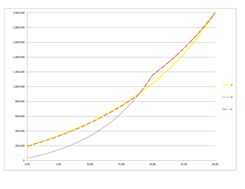
Figure 7: Example 3. The technical interest rate is $\hat{r}=0.05$. The market interest rate is $r(t)=0.10\cdot 1_{(t\leq 20)}+0.04\cdot 1_{(t>20)}$. Surrender is optimal if the surrender value is higher than the market reserve with no surrender.

Example 4: Market interest rate is increasing

Assume $r(t)=0.01\cdot 1_{(t\leq 20)}+0.065\cdot 1_{(t>20)}$. The qualitative feature we capture is that the interest rate crosses the guaranteed interest rate upwards. The reserve developments are displayed in Figure 8. In this situation we have that after time $t=20$ it is optimal to surrender. Before time $t=20$ it is optimal to plan to surrender at time $t=20$. With this strategy the policyholder benefits from both the high market interest rate after time $t=20$ and the technical interest rate before time $t=20$ when the market interest rate is low. Thereby, unlike in the previous three examples, the worst case reserve is no longer the supremum of the surrender value and the market reserve with no surrender. Before time $t=20$ the worst case reserve is higher than both of the other reserves, because there exists a surrender strategy which is better for the policyholder than both immediate surrender and no surrender.

We recall that the reserves of Model a and Model b converge to the worst case reserve when the rationality parameter converges to infinity. Thus, if the rationality parameter is sufficiently high and the future increase in interest rate is sufficiently high, then the reserves of Model a and Model b become higher than the maximum of the surrender value and the market reserve of Model d with no surrender.

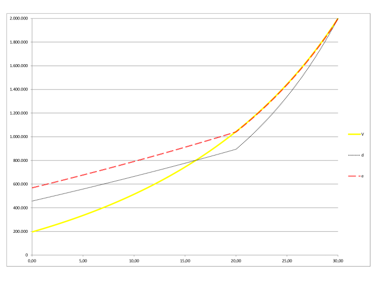
Figure 8: Example 4. The technical interest rate is $\hat{r}=0.05$. The market interest rate is $r(t)=0.01\cdot 1_{(t\leq 20)}+0.065\cdot 1_{(t>20)}$. After time $t=20$ it is optimal to surrender. Before time $t=20$ it is wise to plan to surrender at time $t=20$.

Appendix A Proof of Theorem 5.1

The proof is divided in two parts. One part associated with the risk from the $\nu_{\theta}$ based stopping time surrendering before the optimal time $u^{\ast}$ and another part associated with the risk from the $\nu_{\theta}$ based stopping time surrendering after the optimal time $u^{\ast}$. For this reason we define an intermediate reserve, $W_{\theta}$. The surrender strategy related to $W_{\theta}$ resembles the one related to $V_{\theta}$. The only difference is that the strategy related to $W_{\theta}$ does not surrender before the optimal time. Mathematically we make the following definition. Let $\hat{\tau}_{\theta,t}$ be a stopping time for which the policyholder surrenders at time $u$ with intensity $\nu_{\theta}(u)1_{(u\geq u^{\ast}(t))}$. We may write this stopping time in a convenient way by introducing stopping times, $\hat{\tau}_{\theta,t}^{i}$, given recursively by $\hat{\tau}_{\theta,t}^{0}\equiv 0$ and $\hat{\tau}_{\theta,t}^{i}$ for $i\in{\mathbb{N}}$ surrenders with intensity $\nu_{\theta}(u)1_{(u\geq\hat{\tau}_{\theta,t}^{i-1})}$. With these definitions we get:

$$(I,\hat{\tau}_{\theta,t})\overset{d}{=}(I,\sum_{i=1}^{\infty}\hat{\tau}_{\theta,t}^{i}1_{(\hat{\tau}_{\theta,t}^{i-1}<u^{\ast}(t)\leq\hat{\tau}_{\theta,t}^{i})}).$$

This identity comes from renewal theory and the memoryless property of the exponential distribution. It says that it does not matter if we set the surrender intensity to zero before the optimal time or if we make the policy holder regret her decision every time she is about to surrender before the optimal time. We denote for $s\in[t,n]$ by $W_{\theta}(t,s)$ the reserve at time $s$ associated with the surrender strategy $\hat{\tau}_{\theta,t}$. Then, from the identity above we find that

$$W_{\theta}(t,s)=V(s)+\sum_{i=1}^{\infty}{\mathbb{E}}_{s}\left[e^{-\int_{s}^{\hat{\tau}_{\theta}^{i}}r(u)+\mu(u)du}(G(\hat{\tau}_{\theta}^{i})-V(\hat{\tau}_{\theta}^{i}))1_{(\hat{\tau}_{\theta}^{i-1}\leq u^{\ast}(t)<\hat{\tau}_{\theta}^{i})}\right].$$

Part 1:

First we show that for every $t\in[0,n]$:

$$\liminf_{\theta\rightarrow\infty}V_{\theta}(t)\leq\liminf_{\theta\rightarrow\infty}W_{\theta}(t,t).$$

To prove this we use, given $t\in[0,n]$ and $\varepsilon>0$, the following notation about stopping times, $\tau$:

$$\{\tau\ good\} = \{G(\tau)-V_{\theta}(\tau)\geq 0\},$$

$$\{\tau\ ok\} = \{G(\tau)-V_{\theta}(\tau)\in[-\varepsilon,0)\},$$

$$\{\tau\ bad\} = \{G(\tau)-V_{\theta}(\tau)<-\varepsilon\}.$$

Thus, a stopping time, $\tau$, is called good when it is profitable to surrender at the corresponding time, and it is called bad when the policy holder loses more than $\varepsilon$ on surrendering. In the following, let $u^{\ast}\equiv u^{\ast}(t)$ and let $\hat{\tau}_{\theta}^{i}\equiv\hat{\tau}_{\theta,t}^{i}$. By induction one can show that for every $m\in{\mathbb{N}}$:

$$V_{\theta}(t) = V(t)+{\mathbb{E}}_{t}\left[e^{-\int_{t}^{\hat{\tau}_{\theta}^{1}}r(u)+\mu(u)du}(G(\hat{\tau}_{\theta}^{1})-V(\hat{\tau}_{\theta}^{1}))\right]$$ (9)

$$\geq V(t)$$

$$+\sum_{i=1}^{m}{\mathbb{E}}_{t}\left[e^{-\int_{t}^{\hat{\tau}_{\theta}^{i}}r(u)+\mu(u)du}(G(\hat{\tau}_{\theta}^{i})-V(\hat{\tau}_{\theta}^{i}))1_{(\hat{\tau}_{\theta}^{i-1}\leq u^{\ast}<\hat{\tau}_{\theta}^{i},\hat{\tau}_{\theta}^{1},\ldots,\hat{\tau}_{\theta}^{i-1}ok\ or\ good)}\right]$$

$$+{\mathbb{E}}_{t}\left[e^{-\int_{t}^{\hat{\tau}_{\theta}^{m+1}}r(u)+\mu(u)du}(G(\hat{\tau}_{\theta}^{m+1})-V(\hat{\tau}_{\theta}^{m+1}))1_{(\hat{\tau}_{\theta}^{m}\leq u^{\ast},\hat{\tau}_{\theta}^{1},\ldots,\hat{\tau}_{\theta}^{m}ok\ or\ good)}\right]$$

$$+\sum_{i=1}^{m}{\mathbb{E}}_{t}\left[e^{-\int_{t}^{\hat{\tau}_{\theta}^{i}}r(u)+\mu(u)du}(G(\hat{\tau}_{\theta}^{i})-V(\hat{\tau}_{\theta}^{i}))1_{(\hat{\tau}_{\theta}^{i}\leq u^{\ast},\hat{\tau}_{\theta}^{1},\ldots,\hat{\tau}_{\theta}^{i-1}ok\ or\ good,\hat{\tau}_{\theta}^{i}bad)}\right]$$

$$-\varepsilon\sum_{i=1}^{m}{\mathbb{E}}_{t}\left[e^{-\int_{t}^{\hat{\tau}_{\theta}^{i}}r(u)+\mu(u)du}1_{(\hat{\tau}_{\theta}^{i}\leq u^{\ast},\hat{\tau}_{\theta}^{1},\ldots,\hat{\tau}_{\theta}^{i-1}ok\ or\ good,\hat{\tau}_{\theta}^{i}ok)}\right]$$

The idea is that the reserve $V_{\theta}$ corresponds to the technical reserve, $V$, plus the expected gain from surrender. We investigate what happens if the policyholder regrets to surrender. The impact if the policy holder regrets to surrender at the observed stopping time, $\hat{\tau}_{\theta}^{1}$, depends on whether this stopping time was good, ok or bad. If the stopping time is good, then we know that the value of the gain of surrender is at least as high as waiting for the next time to surrender, and if the stopping time is ok, then we know that the value of the gain of surrender is at most $\varepsilon$ worse than waiting for the next time to surrender. In the above expression we have made these judgements for up to $m$ surrender possibilities before the optimal time.

The sum in the first line corresponds to the case when one of the first $m$ stopping times reaches beyond the optimal time, $u^{\ast}$. The terms of the second line correspond to the case when all of the first $m$ stopping times are before the optimal time, $u^{\ast}$, and they have all been ok or good. In this case, the value of the gain of surrendering at the first stopping time is no higher than waiting for the $m+1$’th stopping time. The sum in the third line corresponds to the case when one of the $m$ first stopping times is bad and is before the optimal time, $u^{\ast}$. The sum of the fourth line is a correction of the $\varepsilon$-small loses from ok stopping times.

If we display the bound relative to $W_{\theta}$ instead of relative to the technical reserve, $V$, then we get the following expression:

$$V_{\theta}(t)$$

$$\geq W_{\theta}(t,t)-\sum_{i=1}^{\infty}{\mathbb{E}}_{t}\left[e^{-\int_{t}^{\hat{\tau}_{\theta}^{i}}r(u)+\mu(u)du}(G(\hat{\tau}_{\theta}^{i})-V(\hat{\tau}_{\theta}^{i}))1_{(\hat{\tau}_{\theta}^{i-1}\leq u^{\ast}<\hat{\tau}_{\theta}^{i},\exists j\in\{1,\ldots,i-1\}:\ \hat{\tau}_{\theta}^{j}bad)}\right]$$

$$-\sum_{i=m+1}^{\infty}{\mathbb{E}}_{t}\left[e^{-\int_{t}^{\hat{\tau}_{\theta}^{i}}r(u)+\mu(u)du}(G(\hat{\tau}_{\theta}^{i})-V(\hat{\tau}_{\theta}^{i}))1_{(\hat{\tau}_{\theta}^{i-1}\leq u^{\ast}<\hat{\tau}_{\theta}^{i},\hat{\tau}_{\theta}^{1},\ldots,\hat{\tau}_{\theta}^{i-1}ok\ or\ good)}\right]$$

$$+{\mathbb{E}}_{t}\left[e^{-\int_{t}^{\hat{\tau}_{\theta}^{m+1}}r(u)+\mu(u)du}(G(\hat{\tau}_{\theta}^{m+1})-V(\hat{\tau}_{\theta}^{m+1}))1_{(\hat{\tau}_{\theta}^{m}\leq u^{\ast},\hat{\tau}_{\theta}^{1},\ldots,\hat{\tau}_{\theta}^{m}ok\ or\ good)}\right]$$

$$+\sum_{i=1}^{m}{\mathbb{E}}_{t}\left[e^{-\int_{t}^{\hat{\tau}_{\theta}^{i}}r(u)+\mu(u)du}(G(\hat{\tau}_{\theta}^{i})-V(\hat{\tau}_{\theta}^{i}))1_{(\hat{\tau}_{\theta}^{i}\leq u^{\ast},\hat{\tau}_{\theta}^{1},\ldots,\hat{\tau}_{\theta}^{i-1}ok\ or\ good,\hat{\tau}_{\theta}^{i}bad)}\right]$$

$$-\varepsilon\sum_{i=1}^{m}{\mathbb{E}}_{t}\left[e^{-\int_{t}^{\hat{\tau}_{\theta}^{i}}r(u)+\mu(u)du}1_{(\hat{\tau}_{\theta}^{i}\leq u^{\ast},\hat{\tau}_{\theta}^{1},\ldots,\hat{\tau}_{\theta}^{i-1}ok\ or\ good,\hat{\tau}_{\theta}^{i}ok)}\right].$$

In the limit of $\theta$, $\varepsilon$ and $m$, then $W_{\theta}$ is the only term which does not converge to 0. To see this, notice that there exists some $K>0$ such that for all $u\in[t,n]$:

$$G(u)-V(u),\in[-K,K],\ \ \text{ and }\ \ G(u)-V_{\theta}(u)\in[-K,K].$$

That is, for any stopping time, the adjustment $G-V$ is bounded by $K$. Thereby we may further bound the value of $V_{\theta}$ by replacing each of these adjustments with $-K$ times an upper bound of the probability of the corresponding event:

$$V_{\theta}(t) \geq W_{\theta}(t,t)-K{\mathbb{P}}_{t}(\exists j\in{\mathbb{N}}:\ \hat{\tau}_{\theta}^{j}bad,\hat{\tau}_{\theta}^{j}\leq u^{\ast})-K\sum_{i=m+1}^{\infty}{\mathbb{P}}_{t}(\hat{\tau}_{\theta}^{i-1}\leq u^{\ast}<\hat{\tau}_{\theta}^{i})$$

$$-K{\mathbb{P}}_{t}(\hat{\tau}_{\theta}^{m}\leq u^{\ast},\hat{\tau}_{\theta}^{1},\ldots,\hat{\tau}_{\theta}^{m}ok\ or\ good)-K{\mathbb{P}}_{t}(\exists j\in{\mathbb{N}}:\ \hat{\tau}_{\theta}^{j}bad,\hat{\tau}_{\theta}^{j}\leq u^{\ast})$$

$$-\varepsilon\sum_{i=1}^{m}{\mathbb{P}}_{t}(\hat{\tau}_{\theta}^{i}\leq u^{\ast},\hat{\tau}_{\theta}^{i}ok)$$

$$\geq W_{\theta}(t,t)-K(1-e^{(n-t)\bar{h}_{\theta}(-\varepsilon)})-K\sum_{i=m+1}^{\infty}{\mathbb{P}}_{t}(\hat{\tau}_{\theta}^{i-1}\leq u^{\ast}<\hat{\tau}_{\theta}^{i})$$

$$-K{\mathbb{P}}_{t}(\hat{\tau}_{\theta}^{m}\leq u^{\ast})-K(1-e^{(n-t)\bar{h}_{\theta}(-\varepsilon)})-\varepsilon n.$$

Given $\theta$ and $\varepsilon$, then this holds for every $n$. Thus, the second sum can be made arbitrarily small and so can ${\mathbb{P}}_{t}(\hat{\tau}_{\theta}^{n}\leq u^{\ast})$, the later follows because given $\theta$, then the intensity of surrender is bounded on $[0,n]$ and thus the distribution of the number of $\hat{\tau}_{\theta}^{i}$ before $u^{\ast}$ is bounded by a Poisson distribution. Thereby:

$$\liminf_{\theta\rightarrow\infty}V_{\theta}(t)\geq\liminf_{\theta\rightarrow\infty}W_{\theta}(t,t).$$

We find from the calculations above that the lower bound holds because the surrender strategy of $W_{\theta}$ and $V_{\theta}$ only differs by the strategy of $W_{\theta}$, regretting every surrender before the optimal time. The impact of this difference is bounded because the following main reasons: The probability of a bad stopping time converges to zero in the limit because of (6). The number of ok or good stopping times occurring before the optimal time is finite. Regret of a good stopping time decreases the value. Regret of an ok stopping time has an impact bounded by $\varepsilon$. At last, the technical calculations justify that the convergence of $\varepsilon$ does not cancel the impact of the convergence of (6).

Part 2:

Consider some arbitrary $t\in[0,n]$. We wish to show that:

$$W_{\theta}(t,t)\rightarrow W(t),\ \ \ \theta\rightarrow.$$

Let $u^{\ast}\equiv u^{\ast}(t)$ and $\hat{\tau}_{\theta}=\hat{\tau}_{\theta,t}$, and notice that since the policyholders related to $W_{\theta}$, $W$ and $V_{\theta}$ behave similarly before time $u^{\ast}$, then convergence at time $t$ corresponds to convergence at time $u^{\ast}$. This is seen from:

$$W(t)-W_{\theta}(t,t) = {\mathbb{E}}_{t}\left[e^{-\int_{t}^{u^{\ast}}r(u)+\mu(u)du}(G(u^{\ast})-V(u^{\ast}))\right.$$

$$\left.-e^{-\int_{t}^{\hat{\tau}_{\theta}}r(u)+\mu(u)du}(G(\hat{\tau}_{\theta})-V(\hat{\tau}_{\theta}))\right]$$

$$= e^{-\int_{t}^{u^{\ast}}r(u)+\mu(u)du}(W(u^{\ast})-W_{\theta}(u^{\ast},u^{\ast}))$$

$$= e^{-\int_{t}^{u^{\ast}}r(u)+\mu(u)du}(W(u^{\ast})-V_{\theta}(u^{\ast})).$$

Thereby, it is sufficient to prove that $V_{\theta}(u^{\ast})\rightarrow W(u^{\ast})$ when $\theta\rightarrow\infty$. Either this holds, or there is some $\varepsilon_{1}>0$ and some sequence $(\theta_{i})_{i\in{\mathbb{N}}}$ converging to infinity such that for all $i\in{\mathbb{N}}$: $V_{\theta_{i}}(u^{\ast})<W(u^{\ast})-2\varepsilon_{1}$. Thereby $V_{\theta_{i}}(u^{\ast})<G(u^{\ast})-2\varepsilon_{1}$.

The derivative of $V_{\theta_{i}}$ is uniformly bounded over $i$ as long as $V_{\theta_{i}}<G$. Thus, there exists some $\delta_{1}$ such that $V_{\theta_{i}}(u)\leq G(u)-\varepsilon_{1}$ for $u\in[u^{*},u^{*}+\delta_{1}]$. For this time interval the gain of surrender compared to waiting is at least $\varepsilon_{1}$, and thereby, for this time interval the intensity for surrender is at least $\underline{h}_{\theta_{i}}(\varepsilon_{1})$.

As $V$ is continuous, then, for every $\varepsilon_{2}>0$, there exists some $\delta_{2}$ such that $(G(u^{*})-V(u^{*}))-e^{-\int_{u^{*}}^{t}r(u)+\mu(u)du}(G(t)-V(t))\leq\varepsilon_{2}$ for $t\in[u^{*},u^{*}+\delta_{2}]$. That is, if surrender happens within time $\delta_{2}$ of the optimal time then the loss of the delay is at most $\varepsilon_{2}$.

Now, let $\delta=\delta_{1}\wedge\delta_{2}$. Then the loss of surrender according to $\hat{\tau}_{\theta_{i}}$ instead of at the optimal time is bounded in the following way:

$$W(u^{\ast})-V_{\theta_{i}}(u^{\ast})$$

$$= {\mathbb{E}}\left[\left.(G(u^{\ast})-V(u^{\ast}))-(G(\hat{\tau}_{\theta_{i}})-V(\hat{\tau}_{\theta_{i}}))e^{-\int_{u^{\ast}}^{\hat{\tau}_{\theta_{i}}}r(x)+\mu(x)dx}\right|\hat{\tau}_{\theta_{i}}\leq\delta\right]{\mathbb{P}}(\hat{\tau}_{\theta_{i}}\leq\delta)$$

$$+{\mathbb{E}}\left[\left.(G(u^{\ast})-V(u^{\ast}))-(G(\hat{\tau}_{\theta_{i}})-V(\hat{\tau}_{\theta_{i}}))e^{-\int_{u^{\ast}}^{\hat{\tau}_{\theta_{i}}}r(x)+\mu(x)dx}\right|(\hat{\tau}_{\theta_{i}}\leq\delta)^{c}\right]{\mathbb{P}}((\hat{\tau}_{\theta_{i}}\leq\delta)^{c})$$

$$\leq \varepsilon_{2}+{\mathbb{E}}\left[\left.(G(u^{\ast})-V(u^{\ast}))-(G(\hat{\tau}_{\theta_{i}})-V(\hat{\tau}_{\theta_{i}}))e^{-\int_{u^{\ast}}^{\hat{\tau}_{\theta_{i}}}r(x)+\mu(x)dx}\right|(\hat{\tau}_{\theta_{i}}\leq\delta)^{c}\right]e^{-\delta\underline{h}_{\theta_{i}}(\varepsilon_{1})}$$

$$\leq \varepsilon_{2}+2Ke^{-\delta\underline{h}_{\theta_{i}}(\varepsilon_{1})}.$$

Thus $V_{\theta_{i}}(u^{\ast})\rightarrow W(u^{\ast})$ as $\theta\rightarrow\infty$, and the result follows.

References

- [1] Bacinello AR (2003) Fair Valuation of a Guaranteed Life Insurance Participating Contract Embedding a Surrender Option. J Risk Insur 70(3):461–487. doi: 10.1111/1539-6975.t01-1-00060
- [2] Buchardt K, Møller T (2013) Life insurance cash flows with policyholder behaviour, Preprint (submitted), available at http://www.math.ku.dk/ buchardt/
- [3] Buchardt K, Møller T, Schmidt KB (2013) Cash flows and policyholder behaviour in the semi-Markov life insurance setup. Scand Actuar J 6:765–798
- [4] Eling M, Kiesenbauer D (2014) What Policy Features Determine Life Insurance Lapse? An analysis of the German Market. J Risk Insur 81(2):241–269. doi: 10.1111/j.1539-6975.2012.01504.x
- [5] Forsyth PA, Vetzal KR (2002) Quadratic convergence for valuing American options using a penalty method. SIAM J Sci Comput 23(6):2095–2122. doi: 10.1137/S1064827500382324
- [6] Gad KST, Pedersen JL (2014). Profit dependent Exercise of the American Put, Preprint, available at arxiv.org/abs/1410.1287
- [7] De Giovanni D (2010). Lapse rate modeling: a rational expectation approach. Scand Actuar J 2010(1):56–67
- [8] Grosen A, Jørgensen PL (2000). Fair Valuation of Life Insurance Liabilities: The Impact of Interest Rate Guarantees, Surrender Options, and Bonus Policies. Insur Math Econ 26(1):37–57
- [9] Henriksen LFB, Nielsen JW, Steffensen M, Svensson C (2014). Markov chain modeling of policyholder behaviour in life insurance and pension. Eur Actuar J 4(1):1–29. doi: 10.1007/s13385-014-0091-2
- [10] Kyprianou A. E. (2006) Introductory Lectures on Fluctuations of Levy Processes with Applications. Springer
- [11] Møller T, Steffensen M (2007) Market-Valuation Methods in Life and Pension Insurance. Cambridge
- [12] Shiryayev AN (1978) Optimal Stopping Rules. Springer-Verlag
- [13] Steffensen M. (2002) Intervention options in life insurance. Insur Math Econ 31:71–85