An Algorithm for Quadratic $\ell_{1}$-Regularized Optimization with a Flexible Active-Set Strategy

Abstract

We present an active-set method for minimizing an objective that is the sum of a convex quadratic and $\ell_{1}$ regularization term. Unlike two-phase methods that combine a first-order active set identification step and a subspace phase consisting of a cycle of conjugate gradient (CG) iterations, the method presented here has the flexibility of computing a first-order proximal gradient step or a subspace CG step at each iteration. The decision of which type of step to perform is based on the relative magnitudes of some scaled components of the minimum norm subgradient of the objective function. The paper establishes global rates of convergence, as well as work complexity estimates for two variants of our approach, which we call the iiCG method. Numerical results illustrating the behavior of the method on a variety of test problems are presented. Index terms— convex optimization, active-set method, nonlinear optimization, lasso

1 Introduction

In this paper, we present an active-set method for the solution of the regularized quadratic problem

$$\min_{x\in\mathbb{R}^{n}}F(x)\stackrel{{\scriptstyle\rm def}}{{=}}\textstyle\frac{1}{2}x^{T}Ax-b^{T}x+\tau{\|x\|}_{1},$$ (1.1)

where $A$ is a symmetric positive semi-definite matrix and $\tau\geq 0$ is a regularization parameter. The motivation for this work stems from the numerous applications in signal processing, machine learning, and statistics that require the solution of problem (1.1); see e.g. [36, 22, 35] and the references therein.

Although non-differentiable, the quadratic-$\ell_{1}$ problem (1.1) has a simple structure that can be exploited effectively in the design of algorithms, and in their analysis. Our focus in this paper is on methods that incorporate second-order information about the objective function $F(x)$ as an integral part of the iteration. A salient feature of our method is the flexibility of switching between two types of steps: a) first-order steps that improve the active-set prediction; b) subspace steps that explore the current active set through an inner conjugate gradient (CG) iteration. The choice between these steps is controlled by the gradient balance condition that compares the norm of the free (non-zero) components of the minimum norm subgradient of $F$ with the norm of the components corresponding to the zero variables (appropriately scaled). This condition is motivated by the work of Dostal and Schoeberl [13] on the solution of bound constrained problems, but in extending the idea to the quadratic-$\ell_{1}$ problem (1.1), we deviate from their approach in a significant way.

We present two variants of our approach that differ in the active set identification step. One variant employs the iterative soft-thresholding algorithm, ISTA [9, 12, 38], while the other computes an ISTA step on the subspace of zero variables. Our numerical tests show that the two algorithms perform efficiently compared to state-of-the-art codes. We provide global rates of convergence as well as work-complexity estimates that bound the total amount of computation needed to achieve an $\epsilon$-accurate solution. We refer to our approach as the “interleaved ISTA-CG method”, or iiCG.

The quadratic-$\ell_{1}$ problem (1.1) has received considerable attention in the literature, and a variety of first and second order methods have been proposed for solving it. Most prominent are variants of the ISTA algorithm and its accelerated versions [27, 3, 4], which have extensive theory and are popular in practice. The TFOCS package [4] provides five first-order methods based on proximal gradient iterations that enjoy optimal complexity bounds; i.e., they achieve $\epsilon$ accuracy in at most $O(1/\sqrt{\epsilon})$ iterations. One of these methods, N83, is tested in our numerical experiments. Other first-order methods for problem (1.1) include LARS [14], coordinate descent [17], a fixed point continuation method [20], and a gradient projection method [15].

Schmidt [32] proposed several scaled sub-gradient methods, which can be viewed as extensions, to quadratic-$\ell_{1}$ problem (1.1), of a projected quasi-Newton method [2], an active-set method [31], and a two-metric projection method [19] for bound constrained optimization. He compares these methods with some first-order methods such as GSPR [15] and SPARSA [38]. We include the best-performing method (PSSgb) in our numerical tests.

Other second order methods have been proposed as well; they compute a step by minimizing a local quadratic model of $F$. Some of these algorithms transform problem (1.1) into a smooth bound constrained quadratic programming problem and apply an interior point procedure [25] or a second order gradient projection algorithm [33, 15]. Methods that are closer in spirit to our approach include FPC_AS [37], orthant-based Newton-CG methods [2, 6, 30], and the semi-smooth Newton method in [26]. Our method differs from all these approaches in the adaptive step-by-step nature of the algorithm, where a different kind of step can be invoked at every iteration. This gives the algorithm the flexibility to adapt itself to the characteristics of the problem to be solved, as we discuss in our numerical tests.

The paper is organized in six sections. In Section 2 we motivate our approach and describe the first algorithm. Section 3 presents the second algorithm. A convergence analysis and a work complexity estimate of the two variants is given in Section 4. Section 5 describes implementation details, such as the use of a line search in the identification phase, and numerical results. The contributions of the paper are summarized in Section 6.

2 The First Algorithm: iiCG-1

Let us define

$$f(x)\stackrel{{\scriptstyle\rm def}}{{=}}\textstyle\frac{1}{2}x^{T}Ax-b^{T}x,\quad\mbox{and}\quad g(x)\stackrel{{\scriptstyle\rm def}}{{=}}\nabla f(x)=Ax-b,$$

so that

$$F(x)=f(x)+\tau{\|x\|}_{1}.$$

Throughout the paper, we assume that $\tau$ is fixed and has been chosen to achieve some desirable properties of the solution of the problem.

The algorithm starts by computing a first-order active-set identification step. Then, a subspace minimization step is computed over the space of free variables (i.e. the non-zero variables given by the first-order step) using the conjugate gradient (CG) method. After each CG iteration, the algorithm determines whether to continue the subspace minimization or perform a first-order step. This decision is based on the so-called gradient balance condition that we now describe.

The iterative soft-thresholding (ISTA) [12, 9] algorithm generates iterates as follows:

$$x^{k+1}=\arg\min_{y}\,m^{k}(y)\stackrel{{\scriptstyle\rm def}}{{=}}\arg\min_{y}f(x^{k})+{(y-x^{k})}^{T}g(x^{k})+\frac{1}{2\alpha}{\|y-x^{k}\|}^{2}+\tau{\|y\|}_{1},$$ (2.1)

where $\alpha>0$ a steplength parameter. Since $m^{k}$ is a separable function, we can write it as

$$x^{k+1} =x^{k}-\alpha\omega(x^{k})-\alpha\psi(x^{k}),$$ (2.2)

where, for $i=1,\ldots,n$,

$$\omega{(x^{k})}_{i} \stackrel{{\scriptstyle\rm def}}{{=}}\left\{\begin{array}[]{lll}0&\mbox{ if }&x^{k}_{i}\neq 0\\ \frac{1}{\alpha}(x^{k}_{i}-\arg\min_{y_{i}}\,m^{k}(y))&\mbox{ if }&x^{k}_{i}=0\\ \end{array}\right\}$$ (2.5)

$$=\left\{\begin{array}[]{lll}0&\mbox{ if }&x^{k}_{i}\neq 0\\ 0&\mbox{ if }&x^{k}_{i}=0\mbox{ and }|g_{i}(x^{k})|\leq\tau\\ g_{i}(x^{k})-\tau\operatorname{sgn}(g_{i}(x^{k}))&\mbox{ if }&x^{k}_{i}=0\mbox{ and }|g_{i}(x^{k})|>\tau\\ \end{array}\right\},$$ (2.9)

$$\quad\psi{(x^{k})}_{i} \stackrel{{\scriptstyle\rm def}}{{=}}\left\{\begin{array}[]{lll}\frac{1}{\alpha}(x^{k}_{i}-\arg\min_{y_{i}}\,m^{k}(y)&\mbox{ if }&x^{k}_{i}\neq 0\\ 0&\mbox{ if }&x^{k}_{i}=0\\ \end{array}\right\}$$ (2.12)

$$=\left\{\begin{array}[]{lll}\frac{1}{\alpha}\left(x^{k}_{i}-\max\{|x^{k}_{i}-\alpha g_{i}(x^{k})|-\alpha\tau,0\}\operatorname{sgn}(x^{k}_{i}-\alpha g_{i}(x^{k}))\right)&\mbox{ if }&x^{k}_{i}\neq 0\\ 0&\mbox{ if }&x^{k}_{i}=0\\ \end{array}\right\}.$$ (2.15)

Following Dostal and Schoeberl [13], we use the magnitudes of the vectors $\omega$ and $\psi$ to determine which type of step should be taken. The vector $\omega(x^{k})$ consists of the components of the minimum norm subgradient of $F$ corresponding to variables at zero (see (4.11)), and its norm provides a first-order estimate of the expected decrease in the objective resulting from changing those variables. Similarly, $\|\psi(x^{k})\|$ provides such an estimate for the free variables, but it is more complex due to the effect of variables changing sign.

Thus, when the magnitude of $\omega(x^{k})$ is large, it is an indication that releasing some of the zero variables can produce substantial improvements in the objective. On the other hand, when $\|\psi(x^{k})\|$ is larger than $\|\omega(x^{k})\|$, it is an indication that a move in the non-zero variables is more beneficial. The algorithm thus monitors the gradient balance condition

$${\|\omega(x^{k})\|}_{2}\leq{\|\psi(x^{k})\|}_{2},$$ (2.16)

which governs the flow of the iteration and distinguishes it from both two-phase methods [2, 6, 38] and semi-smooth Newton methods [26] for problem (1.1).

Let us the describe the algorithm in more detail. The first order step is computed by the ISTA iteration (2.2); see e.g. [6]. The choice of the parameter $\alpha$ is a is discussed below.

The subspace minimization procedure uses the conjugate gradient method to reduce a model of the objective $F(x)$ on the subspace

$$H=\{x|\,x_{i}=0,\quad\mbox{for all $i$ such that }x_{i}^{\rm cg}=0\},$$

where $x^{\rm cg}$ denotes the point at which the CG procedure was started (this point is provided by the ISTA step). The conjugate gradient method is applied to a smooth quadratic function $q$ (as in [37]) that equals the objective $F$ on the current orthant defined by $x^{\rm cg}$, i.e.,

$$q(x;x^{\rm cg})\stackrel{{\scriptstyle\rm def}}{{=}}\textstyle\frac{1}{2}x^{T}Ax+{(-b+\tau\operatorname{sgn}(x^{\rm cg}))}^{T}x,$$ (2.17)

where we use the convention $\operatorname{sgn}(0)=0$ and the fact that

$$\|x\|_{1}=\operatorname{sgn}{(x)}^{T}x.$$ (2.18)

Clearly, $F(x)=q(x;x^{\rm cg})$ for all $x$ such that $\operatorname{sgn}(x)=\operatorname{sgn}(x^{\rm cg})$. The algorithm applies the projected CG iteration [29, chap 16] to the problem

$$\min_{x} \ \ q(x;x^{\rm cg})$$ (2.19)

$${\rm s.t.} \ \ x\in H.$$

The gradient of $q$ at $x^{k}$ on the subspace $H$, is given by $P(g(x^{k})+\tau\operatorname{sgn}(x^{k}))$, where $P$ is the projection onto $H$. It follows that an iteration of the projected CG method is given by

$$x^{k+1} =x^{k}+\alpha_{\rm cg}d^{k},\quad\mbox{with}\quad\alpha_{\rm cg}=\frac{{(r^{k})}^{T}\rho^{k}}{{(d^{k})}^{T}Ad^{k}};$$

$$r^{k+1} =r^{k}+\alpha_{\rm cg}Ad^{k};$$

$$\rho^{k+1} =P(r^{k+1});$$

$$d^{k+1} =-\rho^{k+1}+\frac{{(r^{k+1})}^{T}\rho^{k+1}}{{(r^{k})}^{T}\rho^{k}}d^{k},$$

where initially $r^{k}=g(x^{k})+\tau\operatorname{sgn}(x^{k})$, $\rho^{k}=P(r^{k})$, $d^{k}=-\rho^{k}$.

The gradient balance condition (2.16) is tested after every CG iteration, and if it is not satisfied, the CG loop is terminated. This is a sign that substantial improvements in the objective value can be achieved by releasing some of the zero variables. This loop is also terminated when the CG iteration has crossed orthants and a sufficient reduction in the objective $F$ was not achieved.

A precise description of the method for solving problem (1.1) is given in Algorithm iiCG-1. Here and henceforth $\|\cdot\|$ stands for the $\ell_{2}$ norm, and $v(x)$ denotes the minimum norm subgradient of $F$ at $x$.

Algorithm 1 Algorithm iiCG-1

0:  $A$, $b$, $\tau$, $x^{0}$, $c$, and $\alpha$

1:  $k=0$

2:  loop

3:     $x^{k+1}=x^{k}-\alpha\omega(x^{k})-\alpha\psi(x^{k})$               ISTA step

4:     $k=k+1$

5:     $r^{k}=g(x^{k})+\tau\operatorname{sgn}(x^{k})$, $\rho^{k}=P(r^{k})$, $d^{k}=-\rho^{k}$, $x^{\rm cg}=x^{k}$

6:     loop

7:        if $\|\omega(x^{k})\|>\|\psi(x^{k})\|$ then

8:           break

9:        end if

10:        $x^{k+1}=x^{k}+\frac{(r^{k})^{T}\rho^{k}}{{(d^{k})}^{T}Ad^{k}}d^{k}$                     CG step

11:        $r^{k+1}=r^{k}+\frac{{(r^{k})}^{T}\rho^{k}}{{(d^{k})}^{T}Ad^{k}}Ad^{k}$

12:        if $\operatorname{sgn}(x^{k+1})\neq\operatorname{sgn}(x^{\rm cg})$ and $F(x^{k+1})>F(x^{k})-c{\|v(x^{k})\|}^{2}$  then

13:           $x^{k+1}=$ cutback$(x_{k},x^{\rm cg},d^{k})$

14:           $k=k+1$

15:           break

16:        end if

17:        $\rho^{k+1}=P(r^{k+1})$

18:        $d^{k+1}=-\rho^{k+1}+\frac{{(r^{k+1})}^{T}\rho^{k+1}}{{(r^{k})}^{T}\rho^{k}}d^{k}$

19:        $k=k+1$

20:     end loop

21:  end loop

A common choice for the stepsize is $\alpha=1/L$ (where $L$ is the largest eigenvalue of $A$) and is motivated by the convergence analysis in Section 4. In practice, precise knowledge of $L$ is not needed; in Section 5 we discuss a heuristic way of choosing $\alpha$.

Let us consider Step 13. It can be beneficial to allow the CG iteration to leave the current orthant, as long as the objective $F$ is reduced sufficiently after every CG step. Inspired by the analysis given in Section 4 (see Lemma 4.4), we require that

$$F(x^{k+1})\leq F(x^{k})-c{\|v(x^{k})\|}^{2},$$ (2.20)

for some $c\geq 0$, where $v(x^{k})$ is the minimum norm subgradient of $F$ at $x^{k}$. The CG iteration is thus terminated as follows. If $x^{k+1}$ is the first CG iterate that leaves the orthant, then we either accept it, if it produces the sufficient decrease (2.20) in $F$, or we cut it back to the boundary of the current orthant. On the other hand, if both $x^{k+1}$ and $x^{k}$ lie outside the current orthant and if sufficient decrease is not obtained at $x^{k+1}$, then the algorithm reverts to $x^{k}$. This procedure is given as follows:

cutback$(x_{k},x^{\rm cg},d^{k})$

  if $\operatorname{sgn}(x^{k})=\operatorname{sgn}(x^{\rm cg})$  then

     $\alpha_{b}=\arg\max_{\alpha_{b}}\{\alpha_{b}:\operatorname{sgn}(x^{k}+\alpha_{b}d^{k})=\operatorname{sgn}(x^{\rm cg})\}$

     $x^{k+1}=x^{k}+\alpha_{b}d^{k}$

  else

     $x^{k+1}=x^{k}$

  end if

One of the main benefits of allowing the CG iteration to move across orthant boundaries is that this strategy prevents the generation of unnecessarily short subspace steps. In addition, if the quadratic model (2.17) does not change much as orthants change (for example, when $\tau$ is small), CG steps can be beneficial in spite of the fact that they are based on information from another orthant.

Note that in algorithm iiCG-1 the index $k$ may be incremented multiple times during every outer iteration loop. While it is possible to express the same algorithmic logic in a more conventional way, with a single $k$ increment in each outer iteration, our description emphasizes that every inner CG step and ISTA step require approximately the same amount of computational effort, which is dominated by a matrix-vector product.

The algorithm of Dostal and Schoeberl includes a step along the direction $-\omega(x^{k})$; its goal is release variables when the gradient balance condition does not hold. We have dispensed with this step, as we have observed that it is more effective to release variables through the ISTA iteration.

3 The Second Algorithm: iiCG-2

This method is motivated by the observation that the ISTA step (2.2) often releases too many zero variables. To prevent this, we replace it (under certain conditions) by a subspace ISTA step given by

$$x^{k+1}=x^{k}-\alpha\psi(x^{k}).$$ (3.1)

Here, zero variables are kept fixed and the rest of the variables are updated by the ISTA iteration; see definition (2.15). Thus, (3.1) refines the estimate of the active set without releasing any variables.

The subspace ISTA step (3.1) is performed only when the gradient balance condition (2.16) is satisfied. If (2.16) is not satisfied, releasing some of the zero variables may be beneficial, and the full-space ISTA step (2.2) is taken to allow this. The freedom to choose among two types of active-set prediction steps provides the algorithm with a powerful active set identification mechanism; see the results in Section 5. The choice of the steplength $\alpha$ in (3.1) is discussed in Section 5. A detailed description this method is given in algorithm iiCG-2.

Algorithm 2 Algorithm iiCG-2

0:  $A$, $b$, $\tau$, $x^{0}$, $c$, and $\alpha$

1:  $k=0$

2:  loop

3:     if $\|\omega(x^{k})\|^{2}\leq\|\psi(x^{k})\|^{2}$ then

4:        $x^{k+1}=x^{k}-\alpha\psi(x^{k})$                   Subspace ISTA step

5:     else

6:        $x^{k+1}=x^{k}-\alpha\omega(x^{k})-\alpha\psi(x^{k})$              ISTA step

7:     end if

8:     $k=k+1$

9:     $r^{k}=g(x^{k})+\tau\operatorname{sgn}(x^{k})$, $\rho^{k}=P(r^{k})$, $d^{k}=-\rho^{k}$, $x^{\rm cg}=x^{k}$

10:     loop

11:        if $\|\omega(x^{k})\|^{2}>\|\psi(x^{k})\|^{2}$ then

12:           break

13:        end if

14:        $x^{k+1}=x^{k}+\frac{{(r^{k})}^{T}\rho^{k}}{{(d^{k})}^{T}Ad^{k}}d^{k}$                 CG step

15:        $r^{k+1}=r^{k}+\frac{{(r^{k})}^{T}\rho^{k}}{{(d^{k})}^{T}Ad^{k}}Ad^{k}$

16:        if $\operatorname{sgn}(x^{k+1})\neq\operatorname{sgn}(x^{\rm cg})$ and $F(x^{k+1})>F(x^{k})-c{\|v(x^{k})\|}^{2}$  then

17:           $x^{k+1}=$ cutback$(x_{k},x^{\rm cg},d^{k})$

18:           $k=k+1$

19:           break

20:        end if

21:        $\rho^{k+1}=P(r^{k+1})$

22:        $d^{k+1}=-\rho^{k+1}+\frac{{(r^{k+1})}^{T}\rho^{k+1}}{{(r^{k})}^{T}\rho^{k}}d^{k}$

23:        $k=k+1$

24:     end loop

25:  end loop

4 Convergence Analysis

We establish global convergence for algorithms iiCG-1 and iiCG-2 by showing that their constitutive steps, ISTA, subspace ISTA and CG, provide sufficient decrease in the objective function. We also show a global 2-step Q-linear rate of convergence, and based on the fact that the number of cut CG steps cannot exceed half of the total number of steps, we establish a complexity result. In addition, we establish finite active set identification and termination for the two iiCG methods.

In this section, we assume that $A$ is nonsingular, and denote its smallest and largest eigenvalues by $\lambda$ and $L$, respectively. Thus, for any $x\in\mathbb{R}^{n}$,

$$\lambda\|x\|^{2}\leq x^{T}Ax\leq L\|x\|^{2}.$$

We denote the minimizer of $F$ by $x^{*}$, and in the rest of this section we use the abbreviations

$$v=v(x^{k}),\quad\omega=\omega(x^{k}),\quad\phi=\phi(x^{k}),\quad\psi=\psi(x^{k}),\quad g=g(x^{k}),$$ (4.1)

when convenient. We start by demonstrating a Q-linear decrease in the objective $F$ for every ISTA step.

Lemma 4.1.

The ISTA step,

$$x^{k+1}=\arg\min_{y}m^{k}(y)=x^{k}-\alpha\omega(x^{k})-\alpha\psi(x^{k}),$$

with $0<\alpha\leq 1/L$, satisfies

$$F(x^{k+1})-F(x^{*})\leq(1-\lambda\alpha)(F(x^{k})-F(x^{*})).$$

Proof.

Since $1/\alpha\geq L$, we have that $m^{k}(y)$ defined in (2.1) is a majorizing function for $F$ at $x_{k}$. Therefore,

$$F(x^{k+1}) \leq m^{k}(x^{k+1}).$$

Since $x^{k+1}$ is the minimizer of $m^{k}$, for any $d\in\mathbb{R}^{n}$, we have

$$F(x^{k+1}) \leq m^{k}(x^{k+1})$$

$$\leq m^{k}(x^{k}+\lambda\alpha d)$$

$$=F(x^{k}+\lambda\alpha d)-\textstyle\frac{1}{2}{(\lambda\alpha d)}^{T}A(\lambda\alpha d)+\frac{1}{2\alpha}\|\lambda\alpha d\|^{2}$$

$$\leq F(x^{k}+\lambda\alpha d)+\textstyle\frac{1}{2}\lambda^{2}\alpha(1-\lambda\alpha)\|d\|^{2}.$$ (4.2)

Since $F$ is a strongly convex function with parameter $\lambda$, it satisfies.

$$F(tx+(1-t)y)\leq tF(x)+(1-t)F(y)-\textstyle\frac{1}{2}\lambda t(1-t)\|x-y\|^{2},$$ (4.3)

for any $x,y\in\mathbb{R}^{n}$ and $t\in[0,1]$, see [28, Pages 63-64]. Setting $x\leftarrow x^{k}$, $y\leftarrow x^{*}$, and $t\leftarrow(1-\lambda\alpha)$ (which is valid because $\lambda\alpha\in(0,1]$), inequality (4.3) yields

$$F(x^{k}+\lambda\alpha(x^{*}-x^{k}))\leq\lambda\alpha F(x^{*})+(1-\lambda\alpha)F(x^{k})-\textstyle\frac{1}{2}\lambda^{2}\alpha(1-\lambda\alpha)\|x^{*}-x^{k}\|^{2}.$$ (4.4)

Since (4.2) holds for any $d$, we can set $d=x^{*}-x^{k}$. Substituting (4.4) in (4.2), we conclude that

$$F(x^{k+1})-F(x^{*}) \leq(1-\lambda\alpha)(F(x^{k})-F(x^{*})).$$

∎

We now establish a similar result for the subspace ISTA step (3.1), under the conditions for which it is invoked, namely when the gradient balance condition is satisfied.

Lemma 4.2.

If $\|\omega(x^{k})\|\leq\|\psi(x^{k})\|$ the subspace ISTA step,

$$x^{k+1}=x^{k}-\alpha\psi(x^{k}),$$ (4.5)

with $0<\alpha\leq 1/L$, satisfies

$$F(x^{k+1})-F(x^{*})\leq(1-\textstyle\frac{1}{2}\lambda\alpha)(F(x^{k})-F(x^{*})).$$

Proof.

By the definitions (2.9) and (2.15), we have that $\omega^{T}\psi=0$, and hence $\omega^{T}(x^{k+1}-x^{k})=0$ (Recall the abbreviations (4.1)). Given the pattern of zeros in $x^{k}$, $\omega$ and $\psi$, we have also that $\|x^{k+1}-\alpha\omega\|_{1}=\|x^{k+1}\|_{1}+\alpha\|\omega\|_{1}$. Using these two observations, we have for the full ISTA step,

$$m^{k}(x^{k}-\alpha\omega-\alpha\psi)$$

$$= \,f(x^{k})+{(-\alpha\omega-\alpha\psi)}^{T}g+\frac{1}{2\alpha}\|-\alpha\omega-\alpha\psi\|^{2}+\tau\|x^{k}-\alpha\omega-\alpha\psi\|_{1}$$

$$= \,f(x^{k})+{(x^{k+1}-\alpha\omega-x^{k})}^{T}g+\frac{1}{2\alpha}\|x^{k+1}-\alpha\omega-x^{k}\|^{2}+\tau\|x^{k+1}-\alpha\omega\|_{1}$$

$$= \,f(x^{k})+{(x^{k+1}-x^{k})}^{T}g+\frac{1}{2\alpha}\|x^{k+1}-x^{k}\|^{2}+\tau\|x^{k+1}\|_{1}-\alpha\omega^{T}g+\frac{1}{2\alpha}\|\alpha\omega\|^{2}+\tau\|\alpha\omega\|_{1}$$

$$= \,m^{k}(x^{k+1})-\alpha\omega^{T}g+\frac{1}{2\alpha}\|\alpha\omega\|^{2}+\tau\alpha\omega^{T}\operatorname{sgn}(\alpha\omega)$$

$$= \,m^{k}(x^{k+1})-\frac{\alpha}{2}\|\omega\|^{2},$$ (4.6)

where the last equality follows from the fact that, by (2.9), for all $i$ s.t. $\omega_{i}\neq 0$, we have $\operatorname{sgn}(g_{i})=\operatorname{sgn}(\omega_{i})$, and that $w^{T}w=w^{T}g-\tau\omega^{T}\operatorname{sgn}(g)$.

For the subspace ISTA step (4.5) we have

$$m^{k}(x^{k+1}) =f(x^{k})+{(x^{k+1}-x^{k})}^{T}g+\frac{1}{2\alpha}\|x^{k+1}-x^{k}\|^{2}+\tau\|x^{k+1}\|_{1}$$

$$=f(x^{k})-\alpha\psi^{T}g+\frac{1}{2\alpha}\|\alpha\psi\|^{2}+\tau\|x^{k+1}\|_{1}$$

$$=m^{k}(x^{k})-\alpha\psi^{T}g+\frac{\alpha}{2}\|\psi\|^{2}+\tau\|x^{k+1}\|_{1}-\tau\|x^{k}\|_{1}.$$ (4.7)

We examine the second term on the right hand side. For $j$ such that $x_{j}^{k}=0$ we have $\psi_{j}(x^{k})=0$. On the other hand, for $x_{j}^{k}\neq 0$ definitions (2.2) and (2.1) yield

$$x_{i}^{k+1}=x_{i}^{k}+\alpha\psi_{i}(x^{k})=\arg\min_{y_{i}}f(x^{k})+(y_{i}-x_{i}^{k})g_{i}(x^{k})+\textstyle\frac{1}{2\alpha}{(y_{i}-x_{i}^{k})}^{2}+\tau|y_{i}|.$$

In examining the optimality conditions of this problem there are two cases. If $x_{j}^{k+1}\neq 0$, we obtain $-g_{j}=\psi_{j}+\tau\operatorname{sgn}(x^{k+1}_{j})$. On the other hand, if $x^{k+1}_{j}=0$ we have $-g_{j}=\psi_{j}+\tau\sigma_{j}$ for some $\sigma_{j}\in[-1,1]$. Substituting for $g_{j}$ in (4.7), and using (2.18) gives

$$m^{k}(x^{k+1})= \,m^{k}(x^{k})+\sum_{j:x_{j}^{k+1}\neq 0}\tau\alpha\psi_{j}\operatorname{sgn}(x^{k+1})_{j}+\sum_{j:x_{j}^{k+1}=0}\tau\alpha\psi_{j}\sigma_{j}-\frac{\alpha}{2}\|\psi\|^{2}+\tau\|x^{k+1}\|_{1}-\tau\|x^{k}\|_{1}$$

$$= \,m^{k}(x^{k})+\sum_{j:x_{j}^{k+1}\neq 0}\tau\alpha\psi_{j}\operatorname{sgn}(x^{k+1})_{j}+\sum_{j:x_{j}^{k+1}=0}\tau\alpha\psi_{j}\sigma_{j}-\frac{\alpha}{2}\|\psi\|^{2}$$

$$+\tau{(x^{k}-\alpha\psi)}^{T}\operatorname{sgn}(x^{k+1})-\tau\|x^{k}\|_{1}$$

$$= \,m^{k}(x^{k})+\tau\sum_{j:x_{j}^{k+1}\neq 0}\left[x^{k}_{j}\operatorname{sgn}(x^{k+1})_{j}-|x^{k}_{j}|\right]+\tau\sum_{j:x_{j}^{k+1}=0}\left[x^{k}_{j}\sigma_{j}-|x^{k}_{j}|\right]-\frac{\alpha}{2}\|\psi\|^{2}$$

$$\leq \,m^{k}(x^{k})-\frac{\alpha}{2}\|\psi\|^{2}.$$ (4.8)

Using in turn (4.6), the gradient balance condition $\|\psi\|\geq\|\omega\|$ and (4.8) we have

$$m^{k}(x^{k})-m^{k}(x^{k}-\alpha\omega-\alpha\psi) =m^{k}(x^{k})-m^{k}(x^{k+1})+m^{k}(x^{k+1})-m^{k}(x^{k}-\alpha\omega-\alpha\psi)$$

$$=m^{k}(x^{k})-m^{k}(x^{k+1})+\frac{\alpha}{2}\|\omega\|^{2}$$

$$\leq m^{k}(x^{k})-m^{k}(x^{k+1})+\frac{\alpha}{2}\|\psi\|^{2}$$

$$\leq 2[m^{k}(x^{k})-m^{k}(x^{k+1})].$$

Since $m^{k}(x^{k})=F(x^{k})$, this relation yields

$$m^{k}(x^{k+1})-F(x^{k})\leq\textstyle\frac{1}{2}[m^{k}(x^{k}-\alpha\omega-\alpha\psi)-F(x^{k})].$$

Using this bound, the fact that $m^{k}$ is a majorizing function of $F$, and that $(x^{k}-\alpha\omega-\alpha\psi)$ is a minimizer of $m^{k}$, we have that for any $d\in{R}^{n}$,

$$F(x^{k+1})-F(x^{k}) \leq\frac{1}{2}[m^{k}(x^{k}+\lambda\alpha d)-F(x^{k})]$$

$$=\frac{1}{2}[f(x^{k})+g^{T}(\lambda\alpha d)+\frac{1}{2\alpha}\|\lambda\alpha d\|^{2}+\tau\|x^{k}+\lambda\alpha d\|_{1}-F(x^{k})]$$

$$=\frac{1}{2}[F(x^{k}+\lambda\alpha d)-F(x^{k})-\textstyle\frac{1}{2}{(\lambda\alpha d)}^{T}A(\lambda\alpha d)+\frac{1}{2\alpha}\|\lambda\alpha d\|^{2}]$$

$$\leq\frac{1}{2}[F(x^{k}+\lambda\alpha d)-F(x^{k})+\textstyle\frac{1}{2}\lambda^{2}\alpha(1-\lambda\alpha)\|d\|^{2}].$$ (4.9)

Since $F$ is a strongly convex function with parameter $\lambda$, it satisfies

$$F(x+td)\leq F(x)+t(F(x+d)-F(x))-\textstyle\frac{1}{2}\lambda(1-t)t\|d\|^{2},$$ (4.10)

for any $x,d\in{R}^{n}$ and $t\in[0,1]$. Setting $x\leftarrow x^{k}$, and $t\leftarrow\lambda\alpha$ (which is valid because $\lambda\alpha\in(0,1]$), inequality (4.10) yields

$$F(x^{k}+\lambda\alpha d)\leq\lambda\alpha F(x^{k})+(1-\lambda\alpha)F(x^{k}+d)-\textstyle\frac{1}{2}\lambda^{2}\alpha(1-\lambda\alpha)\|d\|^{2}.$$

Substituting this inequality in (4.9), and setting $d=x^{*}-x^{k}$ we conclude that

$$F(x^{k+1})-F(x^{k}) \leq\frac{1}{2}(\lambda\alpha)(F(x^{k}+d)-F(x^{k}))$$

$$\leq\frac{1}{2}(\lambda\alpha)(F(x^{*})-F(x^{k})),$$

which implies the result. ∎

Next, we analyze the conjugate gradient step. To do so, we first introduce some notation and a technical lemma. The subgradient of $F(x)$ [28], of least norm, is given by

$$v_{i}(x)=\left\{\begin{array}[]{lll}g_{i}(x)+\tau\operatorname{sgn}(x_{i})&\mbox{ if }&x_{i}\not=0\\ 0&\mbox{ if }&x_{i}=0\mbox{ and }|g_{i}(x)|\leq\tau\\ g_{i}(x)-\tau\operatorname{sgn}(g_{i}(x))&\mbox{ if }&x_{i}=0\mbox{ and }|g_{i}(x)|>\tau\\ \end{array}\right\}\mbox{for }\ i=1,\ldots,n.$$ (4.11)

Recalling (2.9), we can write $v(x)=\omega(x)+\phi(x)$, where

$$\phi_{i}(x)\stackrel{{\scriptstyle\rm def}}{{=}}\left\{\begin{array}[]{lll}g_{i}(x)+\tau\operatorname{sgn}(x_{i})&\mbox{ if }&x_{i}\not=0\\ 0&\mbox{ if }&x_{i}=0\\ \end{array}\right\}\mbox{for }\ i=1,\ldots,n.$$ (4.12)

The following result establishes a relationship between $\psi$ and $\phi$.

Lemma 4.3.

For all $x^{k}$, we have that $\|\psi(x^{k})\|\leq\|\phi(x^{k})\|$.

Proof.

We show that $|\psi_{j}|\leq|\phi_{j}|$ for each $j$ such that $x_{j}\neq 0$ (the other components of the two vectors are zero). If $\phi_{j}=\psi_{j}$ the result holds, so assume $\phi_{j}\neq\psi_{j}$. For such $j$, we have that $x_{j}-\alpha\psi_{j}$ minimizes $m_{j}^{k}(y)$, which by (2.1) is given by

$$m_{j}^{k}(y)=f(x^{k})+g_{j}(y-x^{k}_{j})+\textstyle\frac{1}{2\alpha}{(y-x^{k}_{j})}^{2}+|y|,\quad y\in\mathbb{R}.$$

On the other hand, $x_{j}-\alpha\phi_{j}$ minimizes

$$\bar{m}_{j}^{k}(y)\stackrel{{\scriptstyle\rm def}}{{=}}f(x^{k})+g_{j}(y-x^{k}_{j})+\textstyle\frac{1}{2\alpha}{(y-x^{k}_{j})}^{2}+\operatorname{sgn}(x^{k}_{j})y.$$

Thus $m_{j}^{k}(x^{k}_{j}-\alpha\psi_{j})<m_{j}^{k}(x^{k}_{j}-\alpha\phi_{j})$ and $\bar{m}_{j}^{k}(x^{k}_{j}-\alpha\psi_{j})>\bar{m}_{j}^{k}(x^{k}_{j}-\alpha\phi_{j})$, where the inequalities are strict since both functions are strictly convex. Subtracting these inequalities, we have

$$m_{j}^{k}(x^{k}_{j}-\alpha\psi_{j})-\bar{m}_{j}^{k}(x^{k}_{j}-\alpha\psi_{j})<m_{j}^{k}(x^{k}_{j}-\alpha\phi_{j})-\bar{m}_{j}^{k}(x^{k}-\alpha\phi).$$

Therefore,

$$0\leq|x^{k}_{j}-\alpha\psi_{j}|-\operatorname{sgn}(x^{k}_{j})(x^{k}_{j}-\alpha\psi_{j})<|x^{k}_{j}-\alpha\phi_{j}|-\operatorname{sgn}(x^{k}_{j})(x^{k}_{j}-\alpha\phi_{j}),$$ (4.13)

showing that the right hand side is positive, which implies that

$$\operatorname{sgn}(x^{k}_{j})\neq\operatorname{sgn}(x^{k}_{j}-\alpha\phi_{j}).$$ (4.14)

Now note that, since $m^{k}_{j}$ and $\bar{m}^{k}_{j}$ coincide in a neighborhood of $x^{k}_{j}\neq 0$, $\phi_{j}$ and $\psi_{j}$ have the same sign. We then consider two cases. If $\operatorname{sgn}(x^{k}_{j})=\operatorname{sgn}(x^{k}_{j}-\alpha\psi_{j})$, then by (4.14), the displacement $-\alpha\psi_{j}$ must be shorter than $-\alpha\phi_{j}$; therefore, $|\psi_{j}|<|\phi_{j}|$. On the other hand, if $\operatorname{sgn}(x^{k}_{j})\neq\operatorname{sgn}(x^{k}_{j}-\alpha\psi_{j})$, the left side of (4.13) is $2|x^{k}-\alpha\psi_{j}|$. By (4.14), the right side of (4.13) is $2|x^{k}_{j}-\alpha\phi_{j}|$. Thus $2|x^{k}_{j}-\alpha\psi_{j}|<2|x^{k}_{j}-\alpha\phi_{j}|$. Since the displacement $-\alpha\phi_{j}$ produces a point farther from zero than the displacement $-\alpha\psi_{j}$, and since both displacements produce points with signs different from $\operatorname{sgn}(x^{k}_{j})$, we have that $x^{k}_{j}-\alpha\phi_{j}$ is farther from $x^{k}_{j}$ than $x^{k}_{j}-\alpha\psi_{j}$. Therefore, $|\psi_{j}|<|\phi_{j}|$.

∎

We can now show that a conjugate gradient step also guarantees sufficient decrease in the objective function, provided it is not truncated, i.e. that the cutback procedure is not invoked.

Lemma 4.4.

If Algorithms iiCG-1 or iiCG-2 take a full conjugate gradient step from $x^{k}$ to $x^{k+1}$, then

$$F(x^{k+1})\leq F(x^{k})-\beta\|v(x^{k})\|^{2},$$ (4.15)

where $\beta=\min\{c,1/8L\}$, where $c$ is defined in (2.20).

Proof.

If $\operatorname{sgn}(x^{k+1})\neq\operatorname{sgn}(x^{\rm cg})$, then CG steps are accepted only if condition (2.20) is true, and hence (4.15) is satisfied. Otherwise $\operatorname{sgn}(x^{k+1})=\operatorname{sgn}(x^{\rm cg})$, and $F(x^{k+1})=q(x^{k+1})$. Since we assume $x^{k+1}$ is given by a full CG step, it follows that $x^{k+1}$ is the result of a sequence of projected CG steps on problem (2.19), starting at $x^{cg}$. It is well known that a CG iterate $x^{k+1}$ is a global minimizer of $q(\cdot\,;x^{\rm cg})$ in the subspace $S={\rm span}\{d^{k},d^{k-1},\ldots\},$ i.e.,

$$q(x^{k+1})=\min\{q(x^{k}+y):y\in S\}.$$

It is also known that $P(\nabla q(x^{k};x^{\rm cg}))\in S$, see [29, Theorem 5.3], and it follows from (4.12) that $P(\nabla q(x^{k};x^{\rm cg}))=\phi$. Thus,

$$F(x^{k+1})=q(x^{k+1})\leq q(x^{k}-\zeta\phi),$$

for any $\zeta$. Let us choose

$$\zeta=\frac{\phi^{T}\phi}{\phi^{T}A\phi}.$$

Recalling (2.17), we have

$$F(x^{k+1}) \leq\textstyle\frac{1}{2}(x^{k}-\zeta\phi)^{T}A(x^{k}-\zeta\phi)+(-b+\tau\operatorname{sgn}(x^{\rm cg}))^{T}(x^{k}-\zeta\phi)$$

$$=F(x^{k})+\frac{1}{2}\zeta\phi^{T}A\zeta\phi-\zeta\phi^{T}Ax^{k}+(-b+\tau\operatorname{sgn}(x^{\rm cg}))^{T}(-\zeta\phi)$$

$$=F(x^{k})+\frac{\zeta}{2}\|\phi\|^{2}-\zeta\phi^{T}(Ax^{k}-b+\tau\operatorname{sgn}(x^{\rm cg})).$$

By (4.12), for $i$ such that $x_{i}^{k}=0$ we have $\phi_{i}=0$, and for $x_{i}^{k}\neq 0$ we have that $\phi_{i}=(Ax^{k}-b+\tau\operatorname{sgn}(x^{\rm cg}))_{i}$. Therefore,

$$F(x^{k+1}) =F(x^{k})-\frac{\zeta}{2}\|\phi\|^{2}$$

$$\leq F(x^{k})-\frac{1}{2L}\|\phi\|^{2}.$$

Since the step is only taken when condition (2.16) is true, we have from Lemma 4.3 that

$$\|v\|\leq\|\omega\|+\|\phi\|\leq\|\psi\|+\|\phi\|\leq 2\|\phi\|.$$

Therefore, we have that the following bound holds after one CG iteration,

$$F(x^{k+1})\leq F(x^{k})-\frac{1}{8L}\|v\|^{2}.$$ (4.16)

This implies (4.15) by definition of $\beta$. ∎

We can now establish a 2-step $Q$-linear convergence result for both algorithms by combining the properties of their constitutive steps

Theorem 4.5.

Suppose that the stepsize $\alpha$ in the ISTA step (2.2) and the subspace ISTA step (4.5) satisfy $\textstyle\frac{1}{8L}\leq\alpha\leq\textstyle\frac{1}{L}$, and let $\beta=\min\{c,1/8L\}$. Then, for the entire sequence $\{x^{k}\}$ generated by Algorithms iiCG-1 and iiCG-2 we have

$$F(x^{k+2})-F(x^{*})\leq\left(1-\frac{\lambda\beta}{2}\right)(F(x^{k})-F(x^{*})),$$ (4.17)

and thus $\{x^{k}\}\rightarrow x^{*}$.

Proof.

By Lemma 4.1 and the lower bound on $\alpha$, we have that the ISTA step satisfies

$$F(x^{k+1})-F(x^{*})\leq(1-\textstyle\frac{\lambda}{16L})(F(x^{k})-F(x^{*})).$$ (4.18)

By Lemma 4.2, and the lower bound on $\alpha$, we have that the subspace ISTA step also satisfies (4.18). By definition of $\beta$, relation (4.18) implies (4.17).

Now a that full CG steps provide the decrease (4.15). Convexity of $F$ shows that

$$F(x^{k})-F(x^{*})\leq-v^{T}(x^{*}-x^{k})\leq\|v\|\|x^{*}-x^{k}\|,$$

which combined with (4.15) gives

$$F(x^{k})-F(x^{k+1})\geq\beta\frac{(F(x^{k})-F(x^{*}))^{2}}{\|x^{*}-x^{k}\|^{2}}.$$

Furthermore, since $F$ is strongly convex, it satisfies

$$F(x^{k})-F(x^{*})\geq\textstyle\frac{\lambda}{2}\|x^{k}-x^{*}\|^{2},$$

see [28, pp. 63-64]. Using this bound we conclude that full CG steps satisfy (4.17).

Let us assume now that all CG steps terminated by the cutback procedure; i.e., that the worst case happens. After every such shortened CG step which may not provide sufficient reduction in $F$, the algorithm computes an ISTA step. Therefore, the Q-linear decrease (4.18) is guaranteed for every 2 steps, yielding (4.17) for all $k$.

Since the algorithms are descent methods, this implies the entire sequence satisfies $F(x^{k})\rightarrow F(x^{*})$ monotonically. Moreover, since $F$ is strictly convex it follows that $x^{k}\rightarrow x^{*}$. ∎

The most costly computations in our algorithms are matrix-vector products; the rest of the computations consist of vector operations. Therefore, when establishing bounds on the total amount of computation required to obtain an $\epsilon$-accurate solution, it is appropriate to measure work in terms of matrix-vector products. Since there is a single matrix-vector product in each of the constitutive steps of our methods, a work complexity result can be derived from Theorem 4.5.

Corollary 4.6.

The number of matrix-vector products required by algorithms iiCG-1 and iiCG-2 to compute an iterate $\hat{x}$ such that

$$F(\hat{x})-F(x^{*})\leq\epsilon,$$ (4.19)

is at most

$$\log\left[\frac{\epsilon}{F(x^{0})-F(x^{*})}\right]\Big{/}\log\sqrt{1-\textstyle\frac{\lambda\beta}{2}}.$$ (4.20)

Proof.

By (4.17), the condition (4.19), with $\hat{x}=x^{k+2}$, will be satisfied by an integer $k$ such that

$$\left(1-\textstyle\frac{\lambda\beta}{2}\right)^{\frac{k}{2}}(F(x^{0})-F(x^{*}))\leq\epsilon.$$

We obtain (4.20) by solving for $k$. ∎

From the point of view of complexity, choosing $c=1/8L$ is best, but in practice we have found it more effective to use a very small value of $c$ since the strength of the conjugate gradient method is sometimes observed only after a few iterations are computed outside the orthant. More generally, Corollary 4.20 represents worst-case analysis, and is not indicative of the overall performance of the algorithm in practice. In our analysis we used the fact that a CG step is no worse than a standard gradient step – a statement that hides the power of the subspace procedure, which is evident in the finite termination result given next.

To prove that algorithms iiCG-1 and iiCG-2 identify the optimal active manifold and the optimal orthant in a finite number of iterations, we assume that strict complementarity holds. Since $v(x^{*})=0$, it follows from (4.11) that for all $i$ such that $x_{i}^{*}=0$ we must have $|g_{i}(x^{*})|\leq\tau$. We say that the solution $x^{*}$ satisfies strict complementarity if $x_{i}^{*}=0$ implies that $|g_{i}(x^{*})|<\tau$.

Theorem 4.7.

If the solution $x^{*}$ of problem (1.1) satisfies strict complementarity, then for all sufficiently large $k$, the iterates $x^{k}$ will lie in the same orthant and active manifold as $x^{*}$. This implies that iiCG-1 and iiCG-2 identify the optimal solution $x^{*}$ in a finite number of iterations.

Proof.

We start by defining the sets

$$Z^{*}=\{i:x^{*}_{i}=0\},\quad N^{*}=\{i:x^{*}_{i}<0\},\quad P^{*}=\{i:x^{*}_{i}>0\},$$

and the constants

$$\delta_{1}=\min_{i\in N^{*}\cup P^{*}}{\frac{|x_{i}^{*}|}{2}},\quad\delta_{2}=\min_{i\in Z^{*}}\left[\frac{\tau-|g_{i}(x^{*})|}{2}\right].$$

Clearly $\delta_{1}>0$, and by the strict complementarity assumption we have that $\delta_{2}>0$.

Since, from Theorem 4.5 we have that $\{x^{k}\}\rightarrow x^{*}$, there exists an integer $k_{0}$ such that for any $k\geq k_{0}$ we have

$$x^{k}_{i}<-\delta_{1}\ \ \forall i\in N^{*},\quad x^{k}_{i}>\delta_{1}\ \ \forall i\in P^{*}$$

$$|x^{k}_{i}|<\frac{\alpha\delta_{2}}{2}\ \ \forall i\in Z^{*}$$ (4.21)

$$|g_{i}|<\tau-\delta_{2}\ \ \forall i\in Z^{*}.$$ (4.22)

For all such $k$, we have, by (4.22) that $\omega=0$, which implies the behavior of iiCG-1 and iiCG-2 is identical.

Thus, all variables that are positive at the solution will be positive for $k>k_{0}$; and similarly for all negative variables. For the rest of the variables, we consider the ISTA step,

$$x^{k+1}=\max\{|x^{k}-\alpha g|-\alpha\tau,0\}\operatorname{sgn}(x^{k}-\alpha g).$$

Using (4.21) and (4.22), we have that for any $k\geq k_{0}$ and $i\in Z^{*}$,

$$|x_{i}^{k}-\alpha g_{i}|-\alpha\tau \leq|x_{i}^{k}|+|\alpha g_{i}|-\alpha\tau$$

$$\leq\frac{\alpha\delta_{2}}{2}+\alpha(\tau-\delta_{2})-\alpha\tau$$

$$=-\frac{\alpha\delta_{2}}{2}<0.$$

Therefore, for all $i\in Z^{*}$ and all $k\geq k_{0}$, the ISTA step sets $x^{k+1}=0$.

An ISTA step must be taken within $n$ iterations of $k_{0}$, because of the finite termination property of the conjugate gradient algorithm. Therefore there exists a $k_{1}$ such that for any $k\geq k_{1}$, $\operatorname{sgn}(x^{k})=\operatorname{sgn}(x^{*})$, and by (4.22), $\omega=0$. These two facts imply that for $k\geq k_{1}$, once the algorithm enters the CG iteration it will not leave, since the two break conditions cannot be satisfied. Finite termination of CG implies the optimal solution $x^{*}$ will be found in a finite number of iterations. ∎

5 Numerical Results

We developed a MATLAB implementation of algorithms iiCG-1 and iiCG-2, and in the next subsection we compare their performance relative to two well known proximal gradient methods. This allows us to study the algorithmic components of our methods in a controlled setting, and to identify their most promising characteristics. Then we compare, in Section 5.3, our algorithms to four state-of-the-art codes for solving problem (1.1). Our numerical experiments are performed on four groups of test problems with varying characteristics.

Before describing the numerical tests, we introduce the following heuristic that improves the prediction made by ISTA steps. As suggested by Wright et al. [38], the Barzilai-Borwein stepsize with a non-monotone line-search is usually preferable to a constant stepsize scheme, such as ${\alpha}$ in algorithms iiCG-1 and iiCG-2. Thus Line 3 in iiCG-1 and Lines 4 and 6 in iiCG-2 are replaced by the following procedure, where we now write $\psi$ in the form $\psi(x^{k};\alpha_{B})$ to make its dependence on the steplength $\alpha_{B}$ clear.

ISTA-BB-LS Step

1:  $\alpha_{B}=\textstyle\frac{{(x^{k}-x^{k-1})}^{T}(x^{k}-x^{k-1})}{{(x^{k}-x^{k-1})}^{T}A(x^{k}-x^{k-1})}$

2:  repeat

3:     $x_{F}=x^{k}-\alpha_{B}\omega(x^{k})-\alpha_{B}\psi(x^{k};\alpha_{B})$ (when the ISTA step is invoked)  or $x_{F}=x^{k}-\alpha_{B}\psi(x^{k};\alpha_{B})$ (when the reduced ISTA step is invoked)

4:     $\alpha_{B}=\textstyle\frac{\alpha_{B}}{2}$

5:  until $F(x_{F})\leq\max_{i\in\{1\ldots M\}}F^{i}-\alpha_{B}\xi\|x-x_{F}\|^{2}$

6:  $F^{i+1}=F^{i}$ for all $i\in\{1\ldots M-1\}$

7:  $F^{1}=F(x_{F})$

8:  $x^{k+1}=x_{F}$

At the beginning of the overall algorithm, we initialize $M=5$, $\xi=0.005$, and $F^{i}=F(x^{0})$ for $i\in\{1\ldots M\}$. The choice of parameters $M,\xi$ is as in [38]; we did not attempt to fine tune them to our test set.

5.1 Initial Evaluation of the Two New Algorithms

We implemented the following methods.

• iiCG-1

• iiCG-2

• FISTA The Fast Iterative Shrinkage-Thresholding Algorithm [3], using a constant stepsize given by $1/L$.

• ISTA-BB-LS This method is composed purely of the ISTA-BB-LS steps described at the beginning of this section, which are repeated until convergence.

These four methods allow us to perform a per-iteration comparison of the progress achieved by each method. FISTA and ISTA-BB-LS are known to be efficient in practice and serve as a useful benchmark. In algorithms iiCG-1 and iiCG-2 we set $c=10^{-4}$, and set $\alpha=1/L$ in (2.15) when computing the value of $\psi(x^{k})$ used in the gradient balance condition (2.16). As illustrated in Appendix 8, our algorithms are fairly insensitive to the choice of this parameter.

The first three test problems have the following form, which is sometimes called the elastic net regularization problem [39],

$$\min_{x}\textstyle\frac{1}{2}\|y-Bx\|^{2}+\gamma\|x\|^{2}+\tau\|x\|_{1}.$$ (5.1)

The data $y$ and $B$ was obtained from three different data sets that we call spectra, sigrec, and myrand. The sources of these data sets are as follows.

Spectra. The gasoline spectra problem is a regularized linear regression problem [23]; it is available in MATLAB by typing load spectra. This problem has a slightly different form than (5.1) in the sense that $\ell_{1}$ regularization is imposed on all but one of the variables (which represents the constant term in linear regression).

Sigrec. This signal recovery problem is described by Wright et al. [38]. The authors generate random sparse signals, introduce noise, and encode the signals in a lower dimensional vector by applying a random matrix multiplication. We generated an instance using the code by the authors of [38].

Myrand. We generated a random $2000$ variable problem using the following MATLAB commands

ΨΨΨB = randn(1000,2000); y = 2000*randn(1000,1),
ΨΨ

and employed this matrix and vector in (5.1).

The 4th problem in our test set is of the form

$$\min_{x}\textstyle\frac{1}{2}x^{T}Cx-y^{T}x+\gamma{\|x\|}^{2}+\tau{\|x\|}_{1}.$$ (5.2)

Proxnewt. The data for (5.2) was generated by applying the proximal Newton method described in [7] to an $\ell_{1}$ regularized convex optimization problem of the form $\varphi(x)+\tau\|x\|_{1}$, where $\varphi(x)$ is a logistic regression function and the data is given by the gisette test set in the LIBSVM repository [8]. Each iteration of the proximal Newton method computes a step by solving a subproblem of the form (1.1). We extracted one of these subproblems, and added the $\ell_{2}$ regularization term $\gamma\|x\|^{2}$ to yield a problem of the form (5.2).

We created twelve versions of each of the four problems listed above, by choosing different values of $\gamma$ and $\tau$. This allowed us to create problems with various degrees of ill conditioning and different percentages on non-zeros in the solution. In our datasets, the matrices $B$ and $C$ in (5.1) and (5.2) are always rank deficient; therefore, when $\gamma=0$ the Hessians of $f(x)$ are singular.

The following naming conventions are used. The last digit, as in problems

spectras1, $\cdots$ , spectras4,

indicates one of the four values of $\tau$ that were chosen for each problem so as to generate different percentages of non-zeros in the optimal solution. The degree of ill conditioning, which is controlled by $\gamma$, is indicated in the second-to-last character, as in

spectras1,   spectrai1,   spectram1,

which correspond to the singular, ill conditioned and moderately conditioned versions of the problem. The characteristics of the test problems are given in Appendix 7.

Accuracy in the solution is measured by the ratio

$${\tt tol}=\frac{F(x^{k})-F^{*}}{|F^{*}|},$$ (5.3)

where $F^{*}$ is the best known objective value for each problem. Given the nature of the four algorithms listed above, it is easy to compute and report the ratio (5.3) after each matrix-vector product computation. We initialized $x^{0}$ to the zero vector, and imposed a limit of 50,000 matrix-vector products on all the runs.

In Table 1 we report the results for iiCG-1, iiCG-2, FISTA and ISTA-BB-LS on all the test problems. Matrix-Vector product (MV) counts are a reasonable measure of computational work used by these algorithms since they are by far the costliest operations. All algorithms are terminated as soon as the ratio in (5.3) is less than a prescribed constant; in Table 1 we report results for tol$=10^{-4}$, and tol $=10^{-10}$. Dashes signify failures to find a solution after 50,000 matrix-vector products, and bold numbers mark the best-performing algorithm.

We observe from these tables that problems with an intermediate value of $\tau$ (typically) require the largest effort. This suggests that the values of $\tau$ chosen in our tests gave rise to an interesting collection of problems that range from nearly quadratic to highly regularized piecewise quadratic, with the most challenging problems in the middle range. An analysis of the data given in Table 1 indicates that iiCG-2 is the most efficient in these tests, but not uniformly so. Overall, we regard both iiCG-1 and iiCG-2 as promising methods for solving the regularized quadratic problem (1.1).

Table 1: Number of matrix-vector products to reach accuracies tol $=10^{-4}$ and $=10^{-10}$.

	tol $=10^{-4}$				tol $=10^{-10}$
	iiCG-1	iiCG-2	FISTA	ISTA-BB-LS	iiCG-1	iiCG-2	FISTA	ISTA-BB-LS
myrands1	654	297	248	1311	13614	8102	8511	-
myrands2	513	310	163	547	3228	1885	4748	12782
myrands3	118	123	69	86	398	311	1493	540
myrands4	11	12	21	8	18	20	106	17
myrandi1	14	14	31	19	-	-	26183	-
myrandi2	491	297	163	498	3008	1912	4925	13682
myrandi3	111	116	69	86	352	335	1492	596
myrandi4	11	12	21	8	18	20	106	17
myrandm1	14	14	30	19	57	57	236	726
myrandm2	121	108	111	317	1731	728	2437	5483
myrandm3	117	128	68	86	375	359	1433	466
myrandm4	11	12	21	8	18	19	106	17
spectras1	4	4	265	17	-	45888	-	-
spectras2	4	4	264	20	48200	8656	-	-
spectras3	4	4	263	26	5661	2245	-	-
spectras4	4	4	270	22	30896	9170	-	-
spectrai1	4	4	258	23	42	42	29258	12046
spectrai2	4	4	257	26	159	129	33734	-
spectrai3	4	4	256	19	2246	2205	45339	-
spectrai4	60	105	1036	4192	1898	1751	10030	23579
spectram1	2	2	2	2	10	10	1897	17
spectram2	2	2	2	2	15	12	2024	137
spectram3	5	5	51	7	11	11	1445	163
spectram4	100	100	126	175	107	107	4799	545
sigrecs1	2206	1213	446	3522	3635	2283	1338	6687
sigrecs2	1020	589	291	1494	1191	695	696	1737
sigrecs3	105	94	75	72	120	116	296	86
sigrecs4	11	12	25	8	19	20	145	16
sigreci1	8	8	14	10	-	5415	10542	-
sigreci2	2148	1156	442	3515	3526	2190	1350	6955
sigreci3	1095	532	291	1499	1285	637	659	1728
sigreci4	11	12	25	8	19	20	145	16
sigrecm1	8	8	14	10	51	51	114	386
sigrecm2	65	60	61	101	777	297	864	1138
sigrecm3	199	137	103	229	476	365	1301	504
sigrecm4	11	12	25	8	18	19	144	16
proxnewts1	22739	4077	21173	-	40139	10169	-	-
proxnewts2	9522	6871	6423	38233	15782	8436	-	-
proxnewts3	6463	1865	2026	3659	7092	2098	-	8384
proxnewts4	212	191	1582	311	233	213	-	458
proxnewti1	294	336	2795	49932	3267	1100	-	-
proxnewti2	2274	1384	2212	14029	3519	1983	-	24756
proxnewti3	6076	1437	1702	3027	6585	1647	-	6344
proxnewti4	291	160	1499	296	315	175	-	463
proxnewtm1	32	32	881	190	131	112	20319	2382
proxnewtm2	41	36	784	293	139	101	14310	1369
proxnewtm3	237	232	592	492	262	274	12640	720
proxnewtm4	58	50	472	101	70	58	10380	128

Using the data from Table 1, we illustrate in Figure 1 the relative performance of iiCG-1, iiCG-2, FISTA and ISTA-BB-LS, using the Dolan-Moré profiles [11] (based on the number of matrix-vector multiplications required for convergence). While iiCG-1 and iiCG-2 are efficient in the case tol $=10^{-4}$, iiCG-2 demonstrates superior performance in reaching the higher accuracy.

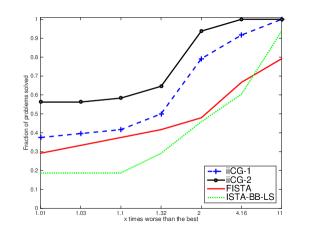
(a) tol = 1e-4

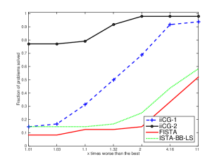
(b) tol = 1e-10

Figure 1: Comparison of the four algorithms using the logarithmic Dolan-Moré profiles, based on the number of matrix-vector products required for convergence. We report results for low and high accuracy (5.3) in the objective function.

In Figure 2 we illustrate typical behavior of iiCG-1 and iiCG-2 by means of problems proxnewts3 and spectram4. We plot the accuracy in the objective (5.3) as a function of of matrix-vector multiplications. Both plots show that our algorithms are able to estimate the solution to high accuracy. They sometimes outperform the other methods from the very start, as in Figure 2(a), but in other cases iiCG-1 and iiCG-2 show their strength later on in the runs; see Figure 2(b). We note that the ISTA-BB-LS method is more efficient than FISTA when high accuracy in the solution is required.

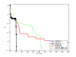
(a) Problem spectram4

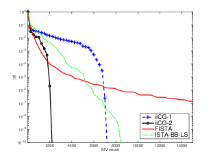
(b) Problem proxnewts3

Figure 2: Accuracy (5.3) in the objective function (vertical axis) as a function of the number of matrix-vector products performed (MV count) performed by each algorithm

We have observed that Algorithm iiCG-2 is superior to iiCG-1 in identifying sparse solutions, due to its judicious application of the subspace ISTA iteration. To illustrate this, we plot in Figure 3 the Pareto frontier based on two quantities: the accuracy (5.3) in the solution, and the number of nonzero elements in the solution. Specifically, we ran the test problems, spectras2 and myrands2 until a specified limit of matrix-vector (MV) products was computed (500, 2100, 30000 for spectras2 and 500, 1000, 2000 for myrands2). For each run, all iterates were considered, and we plotted the pairs (accuracy-nonzeros) such that no other pair existed with both higher accuracy and sparsity. As expected, when more effort (MV) is allowed, higher accuracy is achieved, but not necessarily higher sparsity. As measured by the two quantities depicted in Figure 3, iiCG-2 finds better solutions.

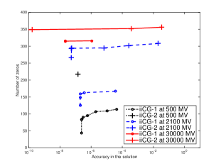
(a) On problem spectras2

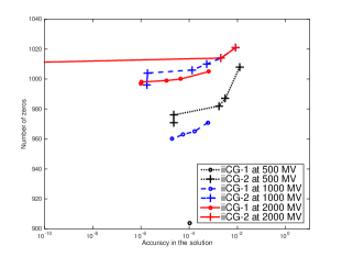
(b) On problem myrands2

Figure 3: Pareto frontier based on the number of nonzeros in the incumbent solution (vertical axis) and accuracy in the solution (5.3) (horizontal axis), for runs imposing 3 limits on the maximum number of matrix-vector (MV) products. The test problems, spectras and myrands2, represent typical behavior of the algorithms.

5.2 Analysis of the CG Phase

We now discuss the behavior of the subspace CG phase, which has a great impact on the overall efficiency of the proposed algorithms. In Figure 4 we report data for two representative runs of iiCG-2 given by test problems myrandm1 and sigreci4. The horizontal axis labels each of the subspace phases invoked by the algorithm, and the vertical axis gives the number of CG iterations performed during that subspace phase.

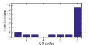
(a) iiCG-2 on sigreci4

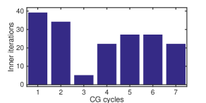
(b) iiCG-2 on myrandm1

Figure 4: Number of CG iterations in each subspace phase

Figure 4(a) illustrates a behavior that is often observed for moderate and large values of the penalty parameter $\tau$, namely that the bulk of the CG iterations are performed towards the end of the run. This is desirable, as the CG phase makes a moderate contribution earlier on towards identifying the optimal active set, and is then able to compute a highly accurate solution of the problem in one (or two) CG cycles. Figure 4(b), considers the case when the penalty parameter $\tau$ is very small, i.e., when $F$ is nearly quadratic. We observe now that the effort expended by the CG phase is more evenly distributed throughout the run. It is reassuring that the number of CG iterations does not tail off for this problem, and that a significant number of CG steps is performed in the last cycle, yielding an accurate solution to the problem.

5.3 Comparisons with Established Codes

We also performed comparisons with the following four state-of-the-art codes. To facilitate our comparisons, and ease of implementation, we only considered codes written in MATLAB.

• SPARSA This is the well known implementation of the ISTA method described in [38]. The code can be found at http://www.lx.it.pt/~mtf/SpaRSA/

• PSSgb The algorithm implemented in this code is motivated by the two-metric projection method [19] for bound constrained optimization. That method is extended to the regularized $\ell_{1}$ problem; curvature information is incorporated in the form of a BFGS matrix. http://www.di.ens.fr/~mschmidt/Software/thesis.html

• N83 Is one of the codes provided by the TFOCS package [4]. It implements the optimal first order Nesterov method described in [27]. http://cvxr.com/tfocs/download/

• pdNCG A Newton-CG method in which the $\ell_{1}$ norm is approximated by a smooth function [16]. http://www.maths.ed.ac.uk/~kfount/index.html

We also experimented with SALSA [1], TWIST [5] and FPC_AS [21], l1_ls [24], YALL1 [10], but these codes were not competitive on our test set with the four packages mentioned above.

In Figure 5 we compare our algorithms with the four codes listed above on all test problems. The figure plots the Dolan-Moré performance profiles based on CPU time; we report results for two values of the convergence tolerance (5.3). Figure 5 indicates that PSSgb is the closest in performance compared to our algorithms.

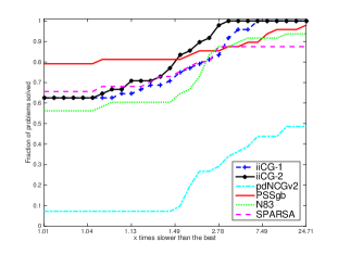
(a) ${\tt tol}=10^{-4}$

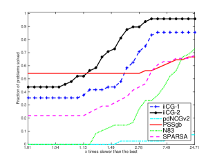
(b) ${\tt tol}=10^{-10}$

Figure 5: Comparison of iiCG-1, iiCG-2, SPARSA, N83 and PSSgb. The figure plots the logarithmic Dolan-Moré performance profiles based on CPU time for problems spectra, sigrec and myrand.

We now examine the behavior of the codes for intermediate values of accuracy. Figure 6 shows the fraction of problems that a method was able to solve faster than the other methods, as a function of the accuracy measure (5.3), in a log-scale.

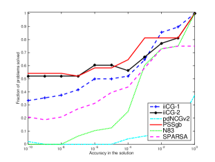
Figure 6: Efficiency. For given accuracy in the function value (horizontal axis), the plot shows the percentage of problems solved to that accuracy within 10% of the time of the best method.

Some algorithms are better suited for problems with a very high solution sparsity. In Figure 7, we show the Dolan-Moré profiles for two sets of problems; one with low sparsity in the solution, and one with high sparsity. The first set of test problems is composed of problems styled name1 (average solution sparsity 25%), and the second is made of problems styled name4 (average solution sparsity 95%). We observe that iiCG-2 outperforms the other codes for low solution sparsity, and that PSSgb is competitive for high sparsity problems. We did not include pdNCGv2 and SPARSA since they are not competitive with the other algorithms, in these tests.

Overall, our iiCG methods are competitive with the four state-of-the-art codes in these tests.

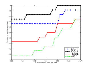
(a) Low Sparsity

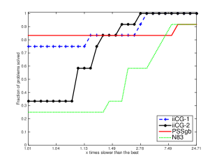
(b) High Sparsity

Figure 7: Comparison of four algorithms using the logarithmic Dolan-Moré profiles, for problems with: low sparsity (Figure a), and high sparsity (Figure b). We set $tol=10^{-7}$

6 Final Remarks

In this paper, we presented a second-order method for solving the $\ell_{1}$ regularized quadratic problem (1.1). We call the method iiCG, for “interleaved ISTA-CG” method. It differs from other second-order methods proposed in the literature in that it can invoke one of two possible steps at each iteration: a subspace conjugate gradient step or a first order active-set identification step. This flexibility is designed to allow the algorithm to adapt itself to the problem to be solved, and the results presented in the paper suggest that it is generally successful at achieving this goal. The decision of what type of step to invoke is based on a measure related to the relative components of the minimum norm subgradient — an idea proposed by Dostal and Schoeberl [13] for the solution of bound constrained quadratic optimization problems. But unlike [13], our algorithm does not include a step along the direction $-\omega(x^{k})$ in order to relax zero variables; as a result our approach departs significantly from the methodology given in [13].

We presented two variants of our method that differ in the first-order active set identification phase. One option uses ISTA, and the other a subspace ISTA iteration.

To provide a theoretical foundation for our method, we established global rates of convergence and complexity bounds based on the total amount of work expended by the algorithm (measured by the total number of matrix-vector products performed). We also gave careful consideration to the main design components of the algorithm, such as the definition of the vectors $\omega,\psi$ employed in the gradient balance condition (2.16). One of the features of the algorithm that was particularly successful is allowing the CG iteration to cross orthants as long as sufficient decrease in the objective function is achieved. The numerical tests reported in this paper suggest that the algorithm proposed in this paper is competitive with state-of-the-art codes.

7 Dataset Details and Sparsity Patterns

The $\tau$ values for each problem were chosen by experimentation so as to span a range of solution sparsities. This is preferable to setting $\tau$ as a multiple of $\|b\|_{\infty}$ (as is often done in the literature based on the fact when $\tau=\|b\|_{\infty}$ the optimal solution to problem (1.1) is the zero vector [18]). We prefer to select the value of $\tau$ for each problem, as there sometimes is a very small range of values that yields interesting problems.

Table 2: myrand $n=2000$

$norm(A)$	$cond(A)$	$\gamma$	problem	$\tau$	num zeros
5781.5	-	0	myrands1	100	1001
			myrands2	1000	1011
			myrands3	10000	1133
			myrands4	100000	1850
5781.5	5.7815e+06	0.001	myrandi1	0.1	583
			myrandi2	100	1011
			myrandi3	10000	1133
			myrandi4	100000	1850
5782.5	5782.5	1	myrandm1	0.1	4
			myrandm2	100	620
			myrandm3	10000	1130
			myrandm4	100000	1850

Table 3: spectra $n=402$

$norm(A)$	$cond(A)$	$\gamma$	problem	$\tau$	num zeros
2.056413e+03	-	0	spectras1	1.0e-06	322
			spectras2	1.0e-04	348
			spectras3	1.0e-03	372
			spectras4	1.0e-02	389
2.056414e+03	2.056414e+06	1.0e-03	spectrai1	3.0e-05	2
			spectrai2	1.0e-03	91
			spectrai3	1.0e-02	313
			spectrai4	5.0e-01	398
2.057413e+03	2.057413e+03	1	spectram1	1.0e-03	1
			spectram2	2.0e-01	109
			spectram3	1	332
			spectram4	30	388

Table 4: sigrec $n=4096$

$norm(A)$	$cond(A)$	$\gamma$	problem	$\tau$	num zeros
1.119904e+00	-	0	sigrecs1	5.0e-05	3549
			sigrecs2	2.0e-04	3816
			sigrecs3	5.0e-03	3860
			sigrecs4	1.0e-01	3973
1.119905e+00	1.119905e+06	1.0e-06	sigreci1	5.0e-08	828
			sigreci2	5.0e-05	3535
			sigreci3	2.0e-04	3813
			sigreci4	1.0e-01	3973
1.120904e+00	1.120904e+03	1.0e-03	sigrecm1	4.5e-07	16
			sigrecm2	1.0e-04	1519
			sigrecm3	2.0e-03	3310
			sigrecm4	1.0e-01	3973

Table 5: proxnewt $n=5000$

$norm(A)$	$cond(A)$	$\gamma$	problem	$\tau$	num zeros
1.103666e+02	-	0	proxnewts1	6.7e-06	1893
			proxnewts2	6.7e-05	3192
			proxnewts3	6.7e-04	4365
			proxnewts4	6.7e-03	4960
1.103667e+02	1.103667e+06	1.0e-04	proxnewti1	6.7e-06	1395
			proxnewti2	6.7e-05	3060
			proxnewti3	6.7e-04	4344
			proxnewti4	6.7e-03	4959
1.103771e+02	1.051211e+04	1.0e-02	proxnewtm1	6.7e-06	193
			proxnewtm2	6.7e-05	1283
			proxnewtm3	6.7e-04	3602
			proxnewtm4	6.7e-03	4926

8 Effect of overestimating $\|A\|$ in the Gradient Balance Condition

In our experiments, we set $\alpha=1/L$ in iiCG, in the gradient balance condition computation. Often $L$ is not known and is hard to compute (for medium and large-scale problems computing $L$ may take longer than running the algorithm itself). Figure 8 shows that while $\alpha=\frac{1}{L}$ is a good choice, iiCG-2 is fairly insensitive to the choice of $\alpha$, particularly if the value $1/L$ is overestimated.

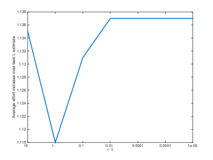
Figure 8: Average increase in matrix-vector products relative to the optimal choice for $\alpha$ (obtained by experimentation), for various choices of $\alpha$. The results are compiled from all 48 test problems, and the runs were stopped when tol=$10^{-4}$ .

References

- [1] M.V. Afonso, J.M. Bioucas-Dias, and M. A T Figueiredo. Fast image recovery using variable splitting and constrained optimization. Image Processing, IEEE Transactions on, 19(9):2345–2356, 2010.
- [2] G. Andrew and J. Gao. Scalable training of -regularized log-linear models. In Proceedings of the 24th international conference on Machine Learning, pages 33–40. ACM, 2007.
- [3] A. Beck and M. Teboulle. A fast iterative shrinkage-thresholding algorithm for linear inverse problems. SIAM Journal on Imaging Sciences, 2(1):183–202, 2009.
- [4] S. R. Becker, E. J. Candés, and M. C. Grant. Templates for convex cone problems with applications to sparse signal recovery. Mathematical Programming Computation, 3(3):165–218, 2011.
- [5] J.M. Bioucas-Dias and M.A.T. Figueiredo. A new TwIST: two-step iterative Shrinkage/Thresholding algorithms for image restoration. IEEE Transactions on Image Processing, 16(12):2992–3004, December 2007.
- [6] R. H. Byrd, G. M. Chin, J. Nocedal, and F. Oztoprak. A family of second-order methods for convex L1 regularized optimization. Technical report, Optimization Center Report 2012/2, Northwestern University, 2012.
- [7] R.H. Byrd, J. Nocedal, and F. Oztoprak. An inexact successive quadratic approximation method for convex l1 regularized optimization. Technical report, Optimization Center, Northwestern University, 2013.
- [8] Chih-Chung Chang and Chih-Jen Lin. LIBSVM: A library for support vector machines. ACM Transactions on Intelligent Systems and Technology, 2:27:1–27:27, 2011. Software available at http://www.csie.ntu.edu.tw/ cjlin/libsvm.
- [9] I. Daubechies, M. Defrise, and C. De Mol. An iterative thresholding algorithm for linear inverse problems with a sparsity constraint. Communications on Pure and Applied Mathematics, 57(11):1413–1457, 2004.
- [10] Wei Deng, Wotao Yin, and Yin Zhang. Group sparse optimization by alternating direction method. TR11-06, Department of Computational and Applied Mathematics, Rice University, 2011.
- [11] E. D. Dolan and J. J. Moré. Benchmarking optimization software with performance profiles. Mathematical Programming, Series A, 91:201–213, 2002.
- [12] D.L. Donoho. De-noising by soft-thresholding. Information Theory, IEEE Transactions on, 41(3):613–627, 1995.
- [13] Z. Dostal and Joachim Schoeberl. Minimizing quadratic functions subject to bound constraints with the rate of convergence and finite termination. Computational Optimization and Applications, 30(1):23–43, 2005.
- [14] Bradley Efron, Trevor Hastie, Iain Johnstone, and Robert Tibshirani. Least angle regression. The Annals of statistics, 32(2), 2004.
- [15] M.A.T. Figueiredo, R.D. Nowak, and S.J. Wright. Gradient projection for sparse reconstruction: Application to compressed sensing and other inverse problems. Selected Topics in Signal Processing, IEEE Journal of, 1(4):586 –597, dec. 2007.
- [16] K. Fountoulakis and J. Gondzio:. A second-order method for strongly-convex l1-regularization problems. Technical Report ERGO-14-005, 2014.
- [17] Jerome Friedman, Trevor Hastie, and Rob Tibshirani. Regularization paths for generalized linear models via coordinate descent. Journal of statistical software, 33(1):1, 2010.
- [18] Jean Jacques Fuchs. More on sparse representations in arbitrary bases. IEEE Trans. on I.T, pages 1341–1344, 2004.
- [19] Eli M. Gafni and Dimitri P. Bertsekas. Two-metric projection methods for constrained optimization. SIAM Journal on Control and Optimization, 22(6):936–964, 1984.
- [20] Elaine T. Hale, Wotao Yin, and Yin Zhang. Fixed-Point Continuation for L1-Minimization: Methodology and Convergence. 2007.
- [21] Elaine T. Hale, Wotao Yin, and Yin Zhang. A fixed-point continuation method for l1-regularized minimization with applications to compressed sensing. CAAM TR07-07, Rice University, 2007.
- [22] Trevor Hastie, Robert Tibshirani, and J. H. Friedman. The elements of statistical learning: data mining, inference, and prediction: with 200 full-color illustrations. New York: Springer-Verlag, 2001.
- [23] John H. Kalivas. Two data sets of near infrared spectra. Chemometrics and Intelligent Laboratory Systems, 37(2):255–259, June 1997.
- [24] Seung-Jean Kim, K. Koh, M. Lustig, S. Boyd, and D. Gorinevsky. An interior-point method for large-scale l1-regularized least squares. Selected Topics in Signal Processing, IEEE Journal of, 1(4):606–617, 2007.
- [25] Seung-Jean Kim, K. Koh, M. Lustig, Stephen Boyd, and Dimitry Gorinevsky. An interior-point method for large-scale l1-control-regularized least squares. IEEE Journal of Selected Topics in Signal Processing, 1(4):606–617, December 2007.
- [26] A. Milzarek and M. Ulbrich. A semismooth Newton method with multi-dimensional filter globalization for L1-optimization. SIAM Journal on Optimization, 24(1):298Ð333, 2014.
- [27] Yurii Nesterov. A method for solving the convex programming problem with convergence rate o(1/k2). Dokl. Akad. Nauk SSSR, 269:543–547, 1983.
- [28] Yurii Nesterov. Introductory Lectures on Convex Optimization: A Basic Course. Boston: Kluwer Academic Publishers, 2004.
- [29] J. Nocedal and S. J. Wright. Numerical Optimization. Springer Series in Operations Research. Springer, second edition, 2006.
- [30] P. Olsen, F. Oztoprak, J. Nocedal, and S. Rennie. Newton-like methods for sparse inverse covariance estimation. In Advances in Neural Information Processing Systems 25, pages 764–772, 2012.
- [31] Simon Perkins, Kevin Lacker, and James Theiler. Grafting: Fast, incremental feature selection by gradient descent in function space. The Journal of Machine Learning Research, 3:1333–1356, 2003.
- [32] Mark Schmidt. Graphical Model Structure Learning with L1-Regularization. PhD thesis, University of British Columbia, 2010.
- [33] Mark Schmidt, Glenn Fung, and Romer Rosales. Fast optimization methods for l1 regularization: A comparative study and two new approaches suplemental material.
- [34] Mark Schmidt, Dongmin Kim, and Sra Suvrit. Projected newton-type methods in machine learning. Optimization for Machine Learning, 2011.
- [35] S. Sra, S. Nowozin, and S.J. Wright. Optimization for Machine Learning. Mit Pr, 2011.
- [36] M.J. Wainwright. Sharp thresholds for high-dimensional and noisy sparsity recovery using -constrained quadratic programming (lasso). Information Theory, IEEE Transactions on, 55(5):2183–2202, May.
- [37] Z. Wen, W. Yin, D. Goldfarb, and Y. Zhang. A fast algorithm for sparse reconstruction based on shrinkage, subspace optimization and continuation. SIAM Journal on Scientific Computing, 32(4):1832–1857, 2010.
- [38] S.J. Wright, R.D. Nowak, and M.A.T. Figueiredo. Sparse reconstruction by separable approximation. IEEE Transactions on Signal Processing, 57(7):2479–2493, 2009.
- [39] Hui Zou and Trevor Hastie. Regularization and variable selection via the elastic net. Journal of the Royal Statistical Society: Series B (Statistical Methodology), 67(2):301–320, 2005.